Pressure Retarded Osmosis Power Units Modelling for Power Flow Analysis of Electric Distribution Networks

Abstract

Pressure retarded osmosis (PRO) power units, which produce electrical energy from salinity gradient sources located at coastlines, are a technology still in the process of maturation; however, there is an expectation that this technology will need to be integrated into electrical distribution networks. Such integration will drive changes in the electric response of the distribution systems which may lead to harmful operating conditions. Power flow analysis is a tool used to reveal the steady-state operating condition of distribution systems and which could be extended to study and address the integration of PRO power units. To the best of the authors’ knowledge, such extension of power flow analysis has not yet been addressed in the literature. Accordingly, this paper comprehensively provides a model to evaluate the electric current and complex power produced by PRO power units. This model is directly embedded in the forward-backward sweep (FBS) method, extending the power flow analysis of electric distribution systems in this way so as to consider the integration of PRO power units. The resulting approach permits revealing of the steady-state operating response of distribution systems and the effects that may be driven by the integration of PRO power units, as corroborated through numerical results on a 14-node test distribution system.

1. Introduction

The concerns about climate change and the depletion of conventional energy sources have driven policies that duly encourage the use of renewable energy resources to harvest electric power. The oceans are a significant source of renewable energy, which can be exploited to produce electric power from waves, tides, ocean currents, and thermal or salinity gradients [1]. This work is related to the use of salinity gradients to produce electric power. A salinity gradient refers to the difference in the salinity concentration between water bodies [2]. Natural sources of salinity gradients are river mouths and hypersaline lagoons [2,3]. To produce electric power from a salinity gradient two water bodies of different salinity concentrations converging at these natural sources must be mixed in a controlled way according to a given mechanism [4].

There are different mechanisms to harvest electric power from a salinity gradient [4], with the most explored being reverse electrodialysis (RED) and pressure retarded osmosis (PRO) [5]. This paper is concerned with the PRO mechanism. In this mechanism, high and low salinity concentration solutions are pumped into bins separated by a semipermeable membrane. The salinity gradient through the membrane creates osmotic pressure that drives the permeation of the low salinity concentration solution into the high salinity concentration solution bin, which is mechanically pressurized to harvest hydraulic power. The recovered hydraulic power is then transformed into electric power by a turbine-electric generator system [2,5,6].

The technical viability of the PRO mechanism to produce electric power from a salinity gradient was first proposed by Sydney Loeb in 1976 [6]. The theoretical worldwide potential of PRO has been estimated to be around 1650 TWh/y [7]. The river mouths with the highest salinity gradient energy potential have been also identified [2]. Due to the significant theoretical energy potential of salinity gradients, the PRO mechanism has been subjected to continuous investigation in the last two decades. A comprehensive review of the technological advances and industrial efforts for commercial production of electric power through this mechanism is duly addressed in [6].

The practical production of electric power employing the PRO mechanism began to manifest through two representative projects. In 2009, the Statkraft PRO pilot plant started producing electric power from a salinity gradient. The power plant was designed for a rated capacity of 10 kW; however, the real power production was only 5 kW [5]. In 2010, a PRO power unit was successfully integrated into the Mega-ton project, where high power densities in the order of 13.5 W/m² were reached [8]. The initial objective of the Mega-ton project was to produce fresh water from seawater desalination; the outcoming high salinity concentration brine water is currently used by the PRO plant, mainly to recover energy and reduce fresh water production costs. Additionally, in 2013, the Statkraft company explored the construction of a 2 MW power plant [5]. It is important to point out that the semipermeable membrane is a critical core feature of harnessing electric power from a salinity gradient [5]. To make feasible electric power production at a commercial level, PRO membranes must be able to provide a power density higher than 6.5 W/m² [9]. The Mega-ton project revealed that it was possible to surpass this technical barrier. In addition, this project proved that electric power can be harvested from hybrid processes, where the salinity gradient is not directly given by a natural source [6,8,9]. Arguably, PRO power is a promising technology to produce electric energy from salinity gradients in a continuous shape, with high expectations for its integration into distribution networks located at coastlines over the next few years [6,9].

Despite the energy potential and the practical manifestations of producing electric power through the PRO mechanism, the modelling and analysis for the integration of PRO power units into electrical networks have not yet been addressed. This issue justifies the proposals in this paper, and will be the focus henceforth.

The power densities of commercial semipermeable membranes clearly suggest that many square meters of membrane surface would be required to assemble a PRO power plant of a capacity in the order of a few megawatts [5]. This issue, along with those of fresh water (low salinity concentration solution) availability and additional environmental constraints may limit the capacity of PRO power units for commercial electric power production to a range from some kilowatts to a few megawatts (see for example [3]). According to the expected capacity of the PRO power units and the definition of distributed generation (DG) [10], the integration of PRO power units to contribute to the electric power supply could be treated as DG. Specifically, PRO power units may be classified in the small DG category, which corresponds to DG units with a rated capacity in the range of 5 kW to 5 MW, where asynchronous generators may be considered due to their lower cost as compared to synchronous generators [10].

The integration of DG to distribution networks is promoted due to a huge list of benefits for governments, owners, electrical utilities and final user entities [11,12,13]. However, integrating DG units is a challenging task for the planning and operation of distribution networks because, depending on the DG technology used and the level of penetration, the performance of the distribution systems may be significantly affected by DG integration [14]. Some of the harmful effects on the system operation caused by DG integration include a reverse flow of power from load nodes to the distribution substation, voltage rise or fluctuations, voltage limit violations through the feeders, overload currents in some components, power quality detriment, increment of the fault currents, and undesired dynamic behavior [10,11,15,16]. These effects become major concerns for the planning and operating stages as they may compromise the reliability and security of the distribution systems [17].

Power flow analysis is a primary tool commonly used in both the operational and planning stages to evaluate the distribution system’s steady-state operating condition, and is also used to assess and develop strategies for improving the performance, reliability, and security of distribution systems [14,16,18]. Hence, to face the problems of planning and operation of distribution systems under the integration of DG units, the formulation of DG models and their incorporation into the power flow analysis is of paramount importance.

Bearing in mind the expectations for integrating PRO power units as DG and the importance of the power flow analysis for the planning and operation of distribution systems, this paper comprehensively addresses the modelling of PRO power units into the power flow analysis of three-phase radial distribution networks. For this purpose, the model of PRO power units reported in [19], assembled by authors of the present work from the basic principles to estimate electric power production [2,20], is adapted and embedded within the formulation of the power flow problem of distribution networks reported in [21]. The resulting power flow problem considering embedded PRO units is directly solved by using the forward-backward sweep (FBS) method [21]. In this way, the proposed approach allows estimating the steady-state performance of distribution systems in the phases reference frame under the integration of PRO power units. Lastly, to the best of the authors’ knowledge, this proposal has not been reported in the literature.

The rest of the paper is organized as follows. In Section 2, the models of conventional components of the distribution network are presented. Section 3 provides the model of the PRO power unit, which is then included within the forward-backward sweep (FBS) method for the power flow analysis of distribution systems presented in Section 4. Section 5 presents the numerical results obtained from the power flow analysis of a distribution system under the integration of PRO power units. Finally, the conclusions and future work lines are discussed in Section 6.

2. Models of Distribution Network Conventional Components

The conventional power flow problem of radial distribution networks aims to assess the nodal voltages, line currents, and complex power flow through the system components for given load demand conditions. In the context of this work, that assessment is extended to consider the power supplied by PRO units connected to the network. For this purpose, a robust technique based on the FBS method should be used such that the well-known approach reported in [21] is adopted. Unlike other methods, the FBS methods are preferred for the analysis of radial distribution systems owing to their simplicity, robustness, and computational speed. It is pointed out that the traditional techniques for the power flow study of transmission networks are not suitable for this task because they exhibit weak convergence when applied to radial distribution networks [22].

The solution of the power flow problem employing the FBS method is achieved by iteratively executing two main stages, referred to as forward and backward sweep steps (as detailed in Section 4). The F-th forward sweep step aims to mainly assess the line-to-ground voltages and the total line currents demanded at every system node. The objective of the B-th backward sweep step is to update the line-to-ground voltages computed in the last previous F-th forward sweep step. For the execution of both main stages, the distribution network components must be classified and modelled as series and shunt components. Bearing this in mind, the models of the conventional components of the distribution system are described below in this section, whereas the modelling of PRO units is addressed in Section 3 in detail.

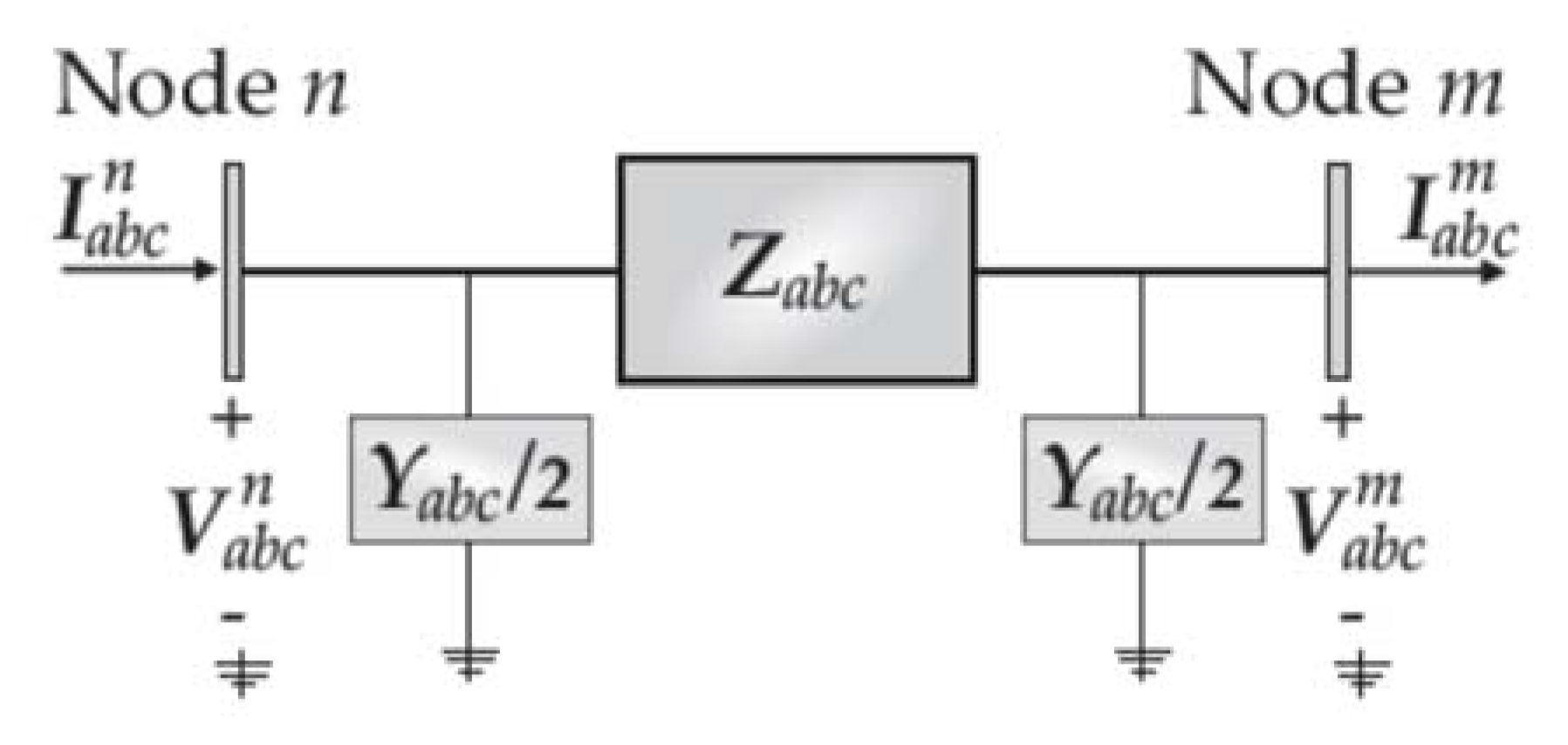
2.1. Modelling of Conventional Series Components

A series component has two terminals connected to two adjacent nodes n and m of the distribution network. Considering the aim of this proposal, the distribution line segments and transformers are the only series components reviewed in this work, and other series elements may be added straightforwardly (see [21]).

Figure 1 depicts a distribution line segment connected between nodes n and m, which is modelled to perform the F-th forward and the B-th backward sweep steps through the algebraic linear systems (1)–(2) and (3), respectively. In this case, ${\mathit{V}}_{abc}^k$ and ${\mathit{I}}_{abc}^k$ denote the sets of line-to-ground voltages and line current phasors at the node k (for k = n,m), respectively. The coefficients a, b, c, d, A and B, are constant matrices computed based on the series impedance Z_abc and shunt admittance Y_abc of the line segment. These two latter matrices are obtained from the parameters of the conductors composing the line segment, as detailed in [21]. Thus, on the one hand, the linear systems (1) and (2) are used in the F-th forward sweep step to assess ${\mathit{V}}_{abc}^n$ and ${\mathit{I}}_{abc}^n$ at node n, respectively, from the phasors ${\mathit{V}}_{abc}^m$ and ${\mathit{I}}_{abc}^m$ at node m. On the other hand, the linear system (3) is used in the B-th backward sweep step to update ${\mathit{V}}_{abc}^m$ at node m from phasors ${\mathit{V}}_{abc}^n$ and ${\mathit{I}}_{abc}^n$ at node n.

$${\mathit{V}}_{abc}^n=\mathit{a}{\mathit{V}}_{abc}^m+\mathit{b}{\mathit{I}}_{abc}^m$$

(1)

$${\mathit{I}}_{abc}^n=\mathit{c}{\mathit{V}}_{abc}^m+\mathit{d}{\mathit{I}}_{abc}^m$$

(2)

$${\mathit{V}}_{abc}^m=\mathit{A}{\mathit{V}}_{abc}^n+\mathit{B}{\mathit{I}}_{abc}^n$$

(3)

Like the distribution line segment, a distribution transformer is modeled for the F-th forward and B-th backward steps through the linear systems (4)–(5) and (6), respectively. In this case, ${\mathit{V}}_{abc}^k$ and ${\mathit{I}}_{abc}^k$ denote the set of line-to-ground voltages and line current phasors at the node k (for k = n,m), respectively, where node n (resp. m) corresponds to the transformer high (resp. low) voltage terminal. In addition, the constant matrices a_t, b_t, c_t, d_t, A_t and B_t are obtained from the nominal ratings, parameters, and type of connection of the transformer, as detailed in [21]. The linear system of Equations (4) and (5) are used in the F-th forward sweep step to assess ${\mathit{V}}_{abc}^n$ and ${\mathit{I}}_{abc}^n$, respectively, at the high voltage terminal (node n) from the known phasors ${\mathit{V}}_{abc}^m$ and ${\mathit{I}}_{abc}^m$ at the low voltage terminal (node m). Note that unlike (3), the set of linear Equations (6) considers the phasors ${\mathit{V}}_{abc}^n$ and ${\mathit{I}}_{abc}^m$ at node n and m, respectively, to update the phasor voltages ${\mathit{V}}_{abc}^m$ at node m in the B-th backward sweep step.

$${\mathit{V}}_{abc}^n={\mathit{a}}_t{\mathit{V}}_{abc}^m+{\mathit{b}}_t{\mathit{I}}_{abc}^m$$

(4)

$${\mathit{I}}_{abc}^n={\mathit{c}}_t{\mathit{V}}_{abc}^m+{\mathit{d}}_t{\mathit{I}}_{abc}^m$$

(5)

$${\mathit{V}}_{abc}^m={\mathit{A}}_t{\mathit{V}}_{abc}^n+{\mathit{B}}_t{\mathit{I}}_{abc}^m$$

(6)

2.2. Modelling of Conventional Shunt Components

A shunt component has only one terminal connected to an adjacent node n of the distribution network, as shown in Figure 2.

At the F-th forward sweep step, the values of line currents ${\mathit{I}}_{abc}^n$ demanded by a shunt component must be evaluated in terms of the line-to-ground voltages ${\mathit{V}}_{abc}^n$ at node n. The power loads are the only conventional shunt components considered in this work. The model for assessing the currents demanded by a power load at the F-th forward sweep step is described in this section. It is highlighted that, unlike series components, shunt components are not involved in backward sweep steps (see Section 4 for details). Thus, the formulation of models for the shunt components, and hence for the power loads, is not required in order to perform backward sweep steps.

At the F-th forward sweep step, the phasors ${\mathit{I}}_{abc}^n$ of the line currents demanded by the load connected to the node n can be computed from the ZIP model given by (7). To assess ${\mathit{I}}_{abc}^n$ from (7), however, the line current components ${\mathit{I}}_{abc\text{\_}Z}^n$, ${\mathit{I}}_{abc\text{\_}I}^n$, and ${\mathit{I}}_{abc\text{\_}P}^n$ must be firstly evaluated by considering the load as a constant impedance, constant current, and constant power, respectively, as explained below. In addition, α, β, and γ in (7) represent the proportion coefficients of these current components, with their constant values selected according to the load characteristics such that the constraint (8) is satisfied.

$${\mathit{I}}_{abc}^n=\alpha {\mathit{I}}_{abc\text{\_}Z}^n+\beta {\mathit{I}}_{abc\text{\_}I}^n+\gamma {\mathit{I}}_{abc\text{\_}P}^n$$

(7)

$$\alpha +\beta +\gamma =1$$

(8)

The values of the line current components ${\mathit{I}}_{abc\text{\_}Z}^n$, ${\mathit{I}}_{abc\text{\_}I}^n$ and ${\mathit{I}}_{abc\text{\_}P}^n$ are assessed at the F-th forward sweep step based on the known phasors ${\mathit{V}}_{abc}^n$ of the line-to-ground voltages at the connecting node n, the complex power, and the type of load connection (i.e., wye or delta), as follows.

For a load in grounded wye connection, the known per phase constant complex power load ${\mathit{S}}_p^n$ (for p = a, b, c) and the line-to-ground voltages ${\mathit{V}}_{abc}^n$ at node n are expressed as in (9). The line current components ${\mathit{I}}_{abc\text{\_}Z}^n$, ${\mathit{I}}_{abc\text{\_}I}^n$ and ${\mathit{I}}_{abc\text{\_}P}^n$ can be evaluated from (10), (11), and (12), respectively, where the per-phase load is considered as a constant impedance ${\mathit{Z}}_p$, constant current magnitude $I_p^n$ and constant complex power ${\mathit{S}}_p^n$, respectively. The per-phase constant impedance ${\mathit{Z}}_p$ and constant current magnitude $I_p^n$ in (10) and (11) are evaluated from (13) and (14), respectively, by considering the initial condition (nominal value) $V_{p\text{\_}0}^n$ of the magnitude of the line-to-ground voltages, the known per phase complex power ${\mathit{S}}_p^n$, and the apparent power $S_p^n$ of the load (for p = a, b, c). Note that the values of ${\mathit{Z}}_p$ and $I_p^n$ are computed at the very beginning of the power flow study and, like ${\mathit{S}}_p^n$ and $S_p^n$, remain constant for the whole study.

$${\mathit{S}}_p^n=P_p^n+j{Q}_p^n=S_p^n\angle {\phi }_p; {\mathit{V}}_{abc}^n=\left[{\mathit{V}}_p^n=V_p^n\angle {\theta }_p\right]; \forall p=a,b,c$$

(9)

$${\mathit{I}}_{abc\text{\_}Z}^n=\left[\raisebox{1ex}{${\mathit{V}}_p^n$}\!\left/ \!\raisebox{-1ex}{${\mathit{Z}}_p$}\right.\right]; \forall p=a,b,c$$

(10)

$${\mathit{I}}_{abc\text{\_}I}^n=\left[I_p^n\angle \left({\theta }_p-{\phi }_p\right)\right]; \forall p=a,b,c$$

(11)

$${\mathit{I}}_{abc\text{\_}P}^n=\left[{\left(\raisebox{1ex}{${\mathit{S}}_p^n$}\!\left/ \!\raisebox{-1ex}{${\mathit{V}}_p^n$}\right.\right)}^{*}\right]; \forall p=a,b,c$$

(12)

$${\mathit{Z}}_p=\raisebox{1ex}{${\left(V_{p\text{\_}0}^n\right)}^2$}\!\left/ \!\raisebox{-1ex}{${\left({\mathit{S}}_p^n\right)}^{*}$}\right.; \forall p=a,b,c$$

(13)

$$I_p^n=\left(\raisebox{1ex}{$S_p^n$}\!\left/ \!\raisebox{-1ex}{$V_{p\text{\_}0}^n$}\right.\right); \forall p=a,b,c$$

(14)

For a load in delta connection, the known per phase constant complex power load ${\mathit{S}}_{\mathsf{\Delta }}^n$ (for Δ = ab, bc, ca) and line-to-ground voltages ${\mathit{V}}_{abc}^n$ at node n are denoted as in (15). To assess the line current components ${\mathit{I}}_{abc\text{\_}Z}^n$, ${\mathit{I}}_{abc\text{\_}I}^n$ and ${\mathit{I}}_{abc\text{\_}P}^n$, the corresponding phase current components ${\mathit{I}}_{abc\text{\_}ZD}^n$, ${\mathit{I}}_{abc\text{\_}ID}^n$, and ${\mathit{I}}_{abc\text{\_}PD}^n$ must first be computed. For this purpose, the phasors ${\mathit{V}}_{abc\text{\_}D}^n$ of the line-to-line voltages must be obtained from transforming the line-to-ground voltages ${\mathit{V}}_{abc}^n$ according to (16), where ${\mathit{D}}_V$ is the transformation matrix given by (17). Then, the phase currents components ${\mathit{I}}_{abc\text{\_}ZD}^n$, ${\mathit{I}}_{abc\text{\_}ID}^n$, and ${\mathit{I}}_{abc\text{\_}PD}^n$ can be assessed from (18), (19), and (20), respectively, where the per-phase load is considered as constant impedance ${\mathit{Z}}_{\mathsf{\Delta }}$, constant current magnitude $I_{\mathsf{\Delta }}^n$, and constant power ${\mathit{S}}_{\mathsf{\Delta }}^n$, respectively. The per-phase constant impedance ${\mathit{Z}}_{\mathsf{\Delta }}$ and constant current magnitude $I_{\mathsf{\Delta }}^n$ are evaluated from (21) and (22), respectively, by considering the initial condition (nominal value) $V_{\mathsf{\Delta }\text{\_}0}^n$ of the magnitude of the line-to-line voltage, the known per phase complex power ${\mathit{S}}_{\mathsf{\Delta }}^n$, and the load apparent power $S_{\mathsf{\Delta }}^n$ (for Δ = ab, bc, ca). The values of ${\mathit{Z}}_{\mathsf{\Delta }}$ and $I_{\mathsf{\Delta }}^n$ must be computed at the very beginning of the power flow study and, like ${\mathit{S}}_{\mathsf{\Delta }}^n$ and $S_{\mathsf{\Delta }}^n$, remain constant for the entire study. Lastly, the line current components ${\mathit{I}}_{abc\text{\_}Z}^n$, ${\mathit{I}}_{abc\text{\_}I}^n$ and ${\mathit{I}}_{abc\text{\_}P}^n$ sought can be evaluated from (23), (24), and (25), respectively, where the phase current components ${\mathit{I}}_{abc\text{\_}ZD}^n$, ${\mathit{I}}_{abc\text{\_}ID}^n$, and ${\mathit{I}}_{abc\text{\_}PD}^n$ are transformed to line currents by using the transformation matrix D_I defined by (26).

$${\mathit{S}}_{\mathsf{\Delta }}^n=P_{\mathsf{\Delta }}^n+j{Q}_{\mathsf{\Delta }}^n=S_{\mathsf{\Delta }}^n\angle {\phi }_{\mathsf{\Delta }}; {\mathit{V}}_{abc}^n=\left[{\mathit{V}}_p^n=V_p^n\angle {\theta }_p\right]; \forall \mathsf{\Delta }=ab, bc, ca;\forall p=a,b,c.$$

(15)

$${\mathit{V}}_{abc\text{\_}D}^n=\left[{\mathit{V}}_{\mathsf{\Delta }}^n=V_{\mathsf{\Delta }}^n\angle {\theta }_{\mathsf{\Delta }}\right]={\mathit{D}}_V{\mathit{V}}_{abc}^n; \forall \mathsf{\Delta }=ab, bc, ca$$

(16)

$${\mathit{D}}_V=\left[\begin{array}{ccc}1& -1& 0\\ 0& 1& -1\\ -1& 0& 1\end{array}\right]$$

(17)

$${\mathit{I}}_{abc\text{\_}ZD}^n=\left[\raisebox{1ex}{${\mathit{V}}_{\mathsf{\Delta }}^n$}\!\left/ \!\raisebox{-1ex}{${\mathit{Z}}_{\mathsf{\Delta }}$}\right.\right]; \forall \mathsf{\Delta }=ab,bc,ca$$

(18)

$${\mathit{I}}_{abc\text{\_}ID}^n=\left[I_{\mathsf{\Delta }}^n\angle \left({\theta }_{\mathsf{\Delta }}-{\phi }_{\mathsf{\Delta }}\right)\right]; \forall \mathsf{\Delta }=ab,bc,ca$$

(19)

$${\mathit{I}}_{abc\text{\_}PD}^n=\left[{\left(\raisebox{1ex}{${\mathit{S}}_{\mathsf{\Delta }}^n$}\!\left/ \!\raisebox{-1ex}{${\mathit{V}}_{\mathsf{\Delta }}^n$}\right.\right)}^{*}\right]; \forall \mathsf{\Delta }=ab,bc,ca$$

(20)

$${\mathit{Z}}_{\mathsf{\Delta }}=\raisebox{1ex}{${\left(V_{\mathsf{\Delta }\text{\_}0}^n\right)}^2$}\!\left/ \!\raisebox{-1ex}{${\left({\mathit{S}}_{\mathsf{\Delta }}^n\right)}^{*}$}\right.; \forall \mathsf{\Delta }=ab,bc,ca$$

(21)

$$I_{\mathsf{\Delta }}^n=\left(\raisebox{1ex}{$S_{\mathsf{\Delta }}^n$}\!\left/ \!\raisebox{-1ex}{$V_{\mathsf{\Delta }\text{\_}0}^n$}\right.\right); \forall \mathsf{\Delta }=ab,bc,ca$$

(22)

$${\mathit{I}}_{abc\text{\_}Z}^n={\mathit{D}}_I{\mathit{I}}_{abc\text{\_}ZD}^n$$

(23)

$${\mathit{I}}_{abc\text{\_}I}^n={\mathit{D}}_I{\mathit{I}}_{abc\text{\_}ID}^n$$

(24)

$${\mathit{I}}_{abc\text{\_}P}^n={\mathit{D}}_I{\mathit{I}}_{abc\text{\_}PD}^n$$

(25)

$${\mathit{D}}_I=\left[\begin{array}{ccc} 1& 0& -1\\ -1& 1& 0\\ 0& -1& 1\end{array}\right]$$

(26)

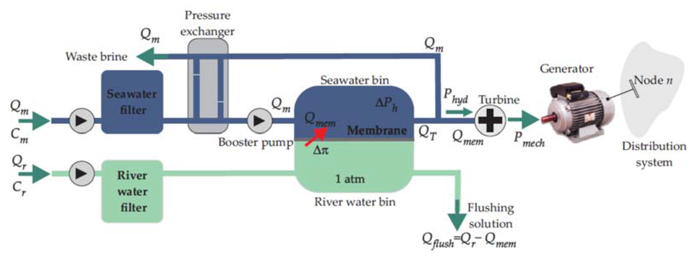
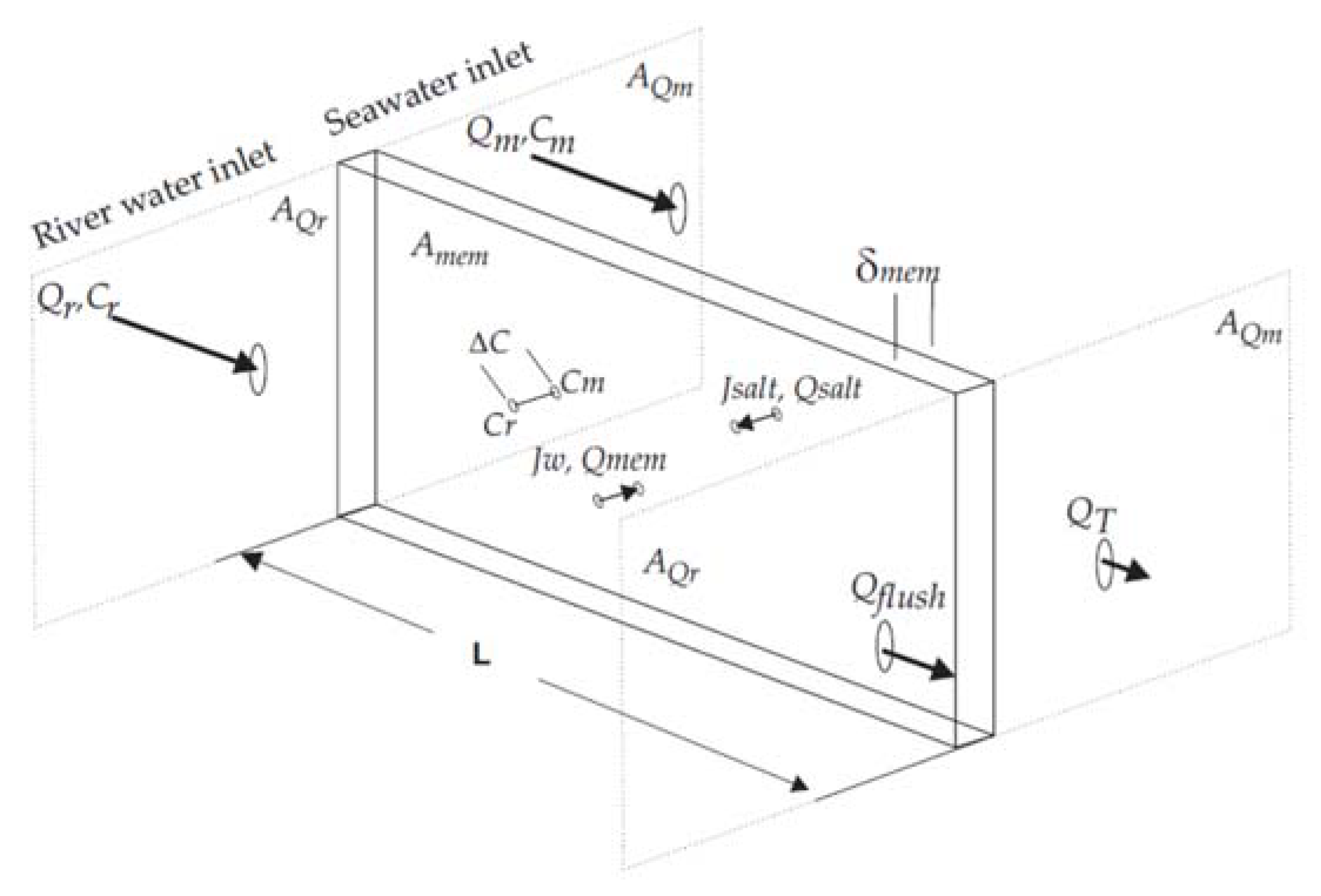
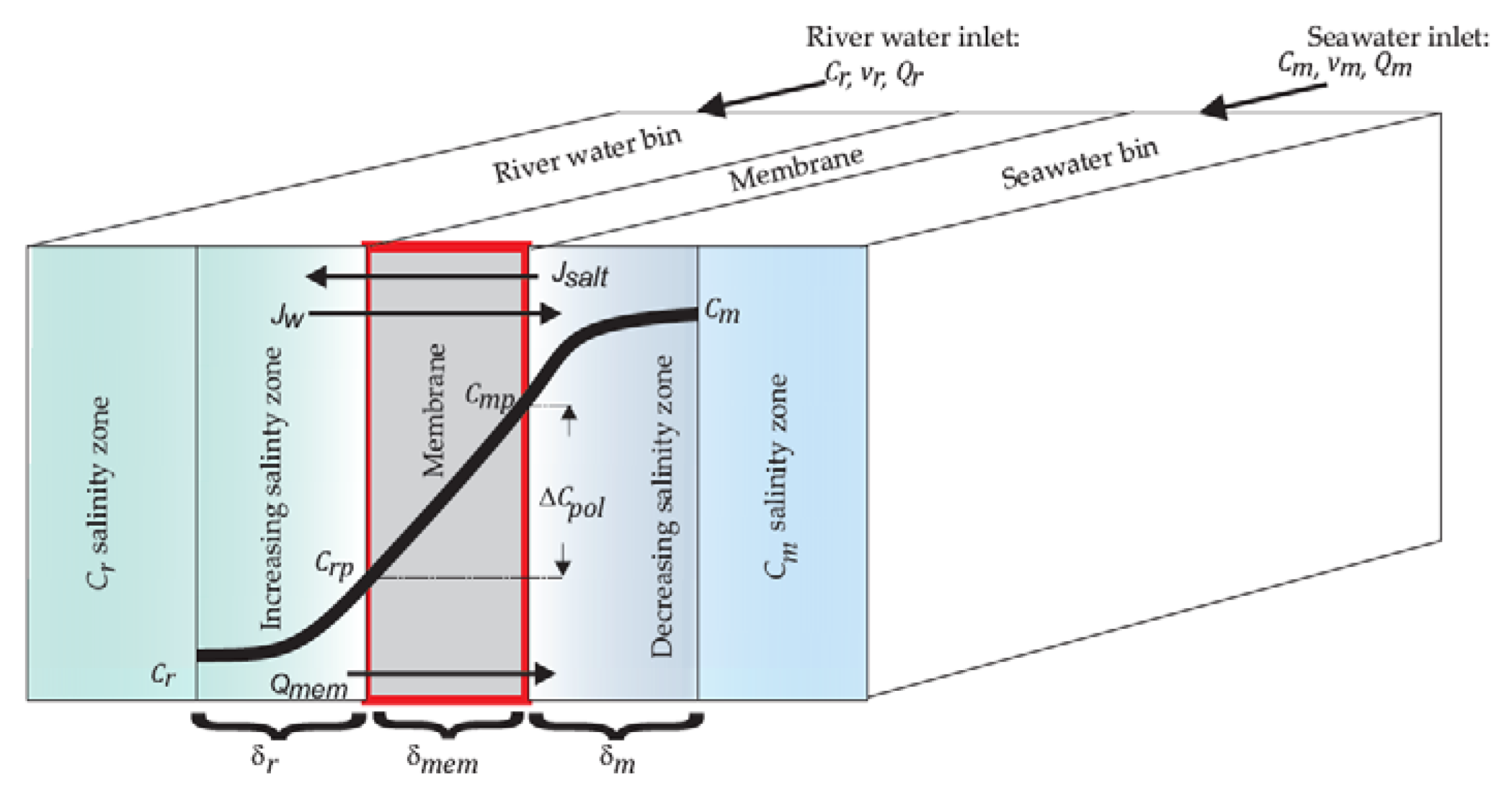
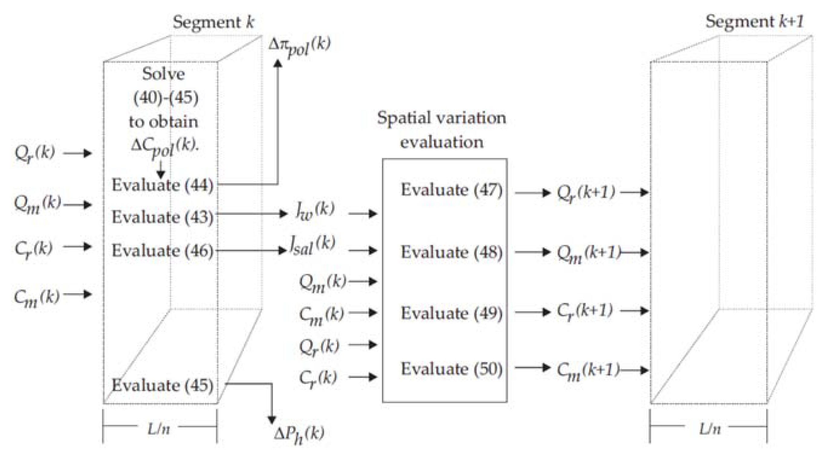
3. Modelling of PRO Power Units

Figure 3 shows the schematic diagram of a PRO power unit with its terminal connected to the adjacent node n. The general process performed by the PRO power unit for generating electric power is as follows. In this power unit, the membrane module uses the high salinity concentration water (seawater) and low salinity concentration water (river water) to harvest hydraulic power from the pressure retarded osmosis mechanism. The turbine transforms this hydraulic power into mechanical power. The resulting mechanical power drives the electric generator to produce electric power, which can be injected into a distribution network to aid in supplying the electric power demand.

To integrate the PRO power unit modelling into the power flow analysis of three-phase radial distribution networks via the FBS method, the PRO power unit can be classified as a shunt component. Accordingly, the model for assessing the line currents injected by the PRO power unit at the connecting node n must be assembled to perform the F-th forward sweep step, which allows for addressing the solution of the power flow problem considering the integration of PRO power units.

Based on the general process of electric power generation mentioned above, the PRO unit current injection model is assembled from the models of the hydraulic power harvested in the membrane module and the mechanical power output of the turbine, and the electric generator model in the phases reference frame, as described below.

3.1. Model of the Harvested Hydraulic Power

The model for assessing the hydraulic power harvested in the membrane module through the pressure retarded osmosis mechanism under ideal conditions is presented below. This model is then extended to consider the polarization and spatial variation of the salinity concentration phenomena [23], which allows a more accurate evaluation of the hydraulic power harvested in the membrane module.

Figure 4 shows the schematic diagram of a membrane module, composed of the river water and seawater bins of cross-sectional area A_Qr and A_Qm, respectively. These bins are separated by a semipermeable membrane of effective permeation area A_mem, length L, and thickness δ_mem. The river water and seawater are pumped into their corresponding bins. The river water bin is at atmospheric pressure, whereas the seawater bin is mechanically pressurized at the hydraulic pressure ΔP_h by means of the external pressure exchanger and the booster pump (see Figure 3). At the inlet of these bins of the membrane module, the pumped river water (resp. seawater) has the salinity concentration and flow rate denoted by C_r (resp. C_m) and Q_r (resp. Q_m), respectively.

The river water and seawater pumped to the membrane module produce through the membrane surfaces the salinity gradient ΔC given by (27) (see Figure 4). This salinity gradient develops the osmotic pressure difference Δπ given by (28), where R, T, M, and i_m denote the universal gas constant, the solution temperature, the molar mass of the salt, and the Van’t Hoff factor, respectively. The osmotic pressure difference Δπ is higher than the opposing hydraulic pressure ΔP_h imposed inside the seawater bin, hence it drives the permeation of river water to the seawater bin through the membrane area A_mem. The permeate flux J_w and the flow rate Q_mem of this river water transference are given by (29) and (30), respectively. In (29), A is the water permeability coefficient. The permeation of the river water at the opposing hydraulic pressure ΔP_h is known as the pressure retarded osmosis mechanism [2,6].

Ideally, the membrane is considered perfectly semipermeable such that salt ions of the seawater are not transferred through the membrane to the river water bin. This assumption implies that the salt mass transferred through the membrane has a flow rate Q_salt and permeate flux J_salt equal to zero. Hence, for this ideal condition, the hydraulic power harvested in the membrane module through the pressure retarded osmosis mechanism can be assessed by the product of the flow rate Q_mem and the opposing hydraulic pressure ΔP_h, as given by (31).

$$\mathsf{\Delta }C=C_m-C_r$$

(27)

$$\mathsf{\Delta }\pi =\raisebox{1ex}{$\mathsf{\Delta }CRT{i}_m$}\!\left/ \!\raisebox{-1ex}{$M$}\right.$$

(28)

$$J_w=A\left(\mathsf{\Delta }\pi -\mathsf{\Delta }{P}_h\right)$$

(29)

$$Q_{mem}=J_w{A}_{mem}$$

(30)

$$P_{hyd}=Q_{mem}\mathsf{\Delta }{P}_h$$

(31)

In (31), the hydraulic power is assessed based on the ideal salinity gradient ΔC given by (27), assuming that the membrane is perfectly semipermeable and that the water and salt mass transference through the membrane can be neglected. However, to carry out a more accurate assessment of the salinity gradient and. eventually, of the hydraulic power, both assumptions can be relaxed by considering the polarization and spatial variation of the salinity concentration phenomena, as described below.

The membrane is not perfectly semipermeable. Hence, through the membrane surfaces, salt ions of the seawater pass to the river water bin at flow rate Q_salt and permeate flux J_salt different from zero, whereas the river water permeates to the seawater bin at flow rate Q_mem and permeate flux J_w. On the one hand, the salt mass transference produces a zone inside the river water bin where the river water salinity concentration increases from the value C_r to a value C_rp at the membrane surface. On the other hand, the river water mass transference produces a zone inside the seawater bin where the seawater salinity concentration decreases from the value C_m to a value C_mp at the membrane surface, as illustrated in the cross-section of the membrane module shown in Figure 5. These zones of different salinity concentrations are referred to as the salinity concentration polarization phenomenon [23]. Accordingly, this phenomenon produces the effective salinity gradient ΔC_pol given by (32). Since C_m > C_mp and C_r < C_rp, the effective salinity gradient ΔC_pol is considerably lower than the ideal one ΔC estimated from (27), as illustrated in Figure 5.

The values of C_mp and C_rp, however, are not known in advance; hence, the effective salinity gradient ΔC_pol must be estimated from the solution of the non-linear Equation (33), where $g\left(\mathsf{\Delta }{C}_{pol}\right)$ and $f\left(\mathsf{\Delta }{C}_{pol}\right)$ are the functions given by (34) and (35). According to (28) and (29), the water permeate flux $J_w$ depends on the salinity gradient through the membrane surfaces. Arguably, due to the polarization phenomenon, that salinity gradient must be considered as ΔC_pol instead of the ideal one ΔC. Thus, in (34) and (35) $J_w$ is expressed as the function of ΔC_pol given by (36), where $\mathsf{\Delta }{\pi }_{pol}$ and ΔP_h are given by (37) and (38), respectively. In these equations, S, δ_j, and D_j represent the membrane structure parameter, the thickness of the salinity increasing and decreasing zones (see Figure 5), and the salt diffusion coefficient (for j = r,m), which are detailed in [23]. In addition, B is the salt permeability coefficient, whereas C_r, C_m, R, T, i_m, and M are those previously denoted for (27) and (28). Once ΔC_pol is obtained from the solution of (33), the river water permeate flux $J_w$, the osmotic pressure $\mathsf{\Delta }{\pi }_{pol}$, the hydraulic pressure ΔP_h, and the salt permeate flux J_salt can be evaluated from (36), (37), (38), and (39), respectively.

$$\mathsf{\Delta }{C}_{pol}=C_{mp}-C_{rp}$$

(32)

$$\mathsf{\Delta }{C}_{pol}·g\left(\mathsf{\Delta }{C}_{pol}\right)-f\left(\mathsf{\Delta }{C}_{pol}\right)=0$$

(33)

$$f\left(\mathsf{\Delta }{C}_{pol}\right)=C_m\exp \left(\frac{-J_w\left(\mathsf{\Delta }{C}_{pol}\right){\delta }_m}{D_m}\right)-C_r\exp \left(\frac{J_w\left(\mathsf{\Delta }{C}_{pol}\right)\left({\delta }_r+S\right)}{D_r}\right)$$

(34)

$$g\left(\mathsf{\Delta }{C}_{pol}\right)=1-\frac{B}{J_w}\left[\exp \left(\frac{-J_w\left(\mathsf{\Delta }{C}_{pol}\right){\delta }_m}{D_m}\right)-\exp \left(\frac{J_w\left(\mathsf{\Delta }{C}_{pol}\right)\left({\delta }_r+S\right)}{D_r}\right)\right]$$

(35)

$$J_w\left(\mathsf{\Delta }{C}_{pol}\right)=A\left(\mathsf{\Delta }{\pi }_{pol}-\mathsf{\Delta }{P}_h\right)$$

(36)

$$\mathsf{\Delta }{\pi }_{pol}=\raisebox{1ex}{$\mathsf{\Delta }{C}_{pol}RT{i}_m$}\!\left/ \!\raisebox{-1ex}{$M$}\right.$$

(37)

$$\mathsf{\Delta }{P}_h=\raisebox{1ex}{$0.5\mathsf{\Delta }{C}_{pol}RT{i}_m$}\!\left/ \!\raisebox{-1ex}{$M$}\right.$$

(38)

$$J_{salt}\left(\mathsf{\Delta }{C}_{pol}\right)=B\mathsf{\Delta }{C}_{pol}$$

(39)

The effective salinity gradient ΔC_pol is obtained from the solution of (33) by assuming that the river water and seawater salinity concentrations C_r and C_m, respectively, remain constant along the membrane length. However, the mass transference of river water and salt occurs gradually through the membrane. Accordingly, the water (resp. salt) total mass inside the river water bin gradually decays (resp. increases), whereas progressively increases (resp. decays) in the seawater bin. This mainly produces gradual spatial variations of the flow rates Q_r and Q_m, the permeate fluxes J_w and J_salt, the salinity concentrations C_r and C_m, and the effective salinity gradient ΔC_pol along the membrane length L. The gradual variation of these variables owing to the progressive mass transference of river water and salt along the membrane is known as the spatial variation phenomenon [23].

To evaluate the spatial variation phenomenon, the membrane module is partitioned into n segments of equal length L_s = L/n and the values of the variables for each segment are then computed, as detailed below. Figure 6 depicts two consecutive segments. Consider that the values of the flow rates and salinity concentrations Q_j(k) and C_j(k) (for j = r,m), respectively, are known at the input of the k-th segment. Take these values to solve (40)–(45) for ΔC_pol(k). Once ΔC_pol(k) is obtained, the values of the osmotic pressure Δπ(k) and the permeate flux J_w(k) and J_salt(k) at the k-th segment can be directly computed from (44), (43) and (46), respectively. Using Q_j(k) and C_j(k), as well as the resulting values of J_w(k) and J_salt(k), the flow rates and salinity concentrations Q_j(k + 1) and C_j(k + 1) (for j = r,m), respectively, at the input of the (k + 1)-th segment must be evaluated from the model (47)–(50), as illustrated in Figure 6. To compute the spatial variations along the membrane length, the (k + 1)-th segment is set as the k-th segment and this process is repeated until processing the last (n-th) segment. Clearly, this procedure starts at the first segment, i.e., for k = 1, where the values of Q_j(k = 1) and C_j(k = 1) are known. Note that the model (40)–(45) corresponds to the discretized form of (33)–(38). Furthermore, in (45) the value of the effective salinity gradient is fixed at the value $\mathsf{\Delta }{C}_{pol}\left(k=1\right)$ computed at the very first segment, in order to neglect the pressure losses along the membrane module.

Lastly, the values of the osmotic pressure Δπ(k) and the hydraulic pressure ΔP_h(k) computed during the evaluation of the spatial variation phenomenon are used to perform an accurate evaluation of the hydraulic power from (51).

$$\mathsf{\Delta }{C}_{pol}\left(k\right)·g\left(\mathsf{\Delta }{C}_{pol}\left(k\right)\right)-f\left(\mathsf{\Delta }{C}_{pol}\left(k\right)\right)=0$$

(40)

$$f\left(\mathsf{\Delta }{C}_{pol}\left(k\right)\right)=C_m\exp \left(\frac{-J_w\left(\mathsf{\Delta }{C}_{pol}\left(k\right)\right){\delta }_m}{D_m}\right)-C_r\exp \left(\frac{J_w\left(\mathsf{\Delta }{C}_{pol}\left(k\right)\right)\left({\delta }_r+S\right)}{D_r}\right)$$

(41)

$$g\left(\mathsf{\Delta }{C}_{pol}\left(k\right)\right)=1-\frac{B}{J_w}\left[\exp \left(\frac{-J_w\left(\mathsf{\Delta }{C}_{pol}\left(k\right)\right){\delta }_m}{D_m}\right)-\exp \left(\frac{J_w\left(\mathsf{\Delta }{C}_{pol}\left(k\right)\right)\left({\delta }_r+S\right)}{D_r}\right)\right]$$

(42)

$$J_w\left(\mathsf{\Delta }{C}_{pol}\left(k\right)\right)=A\left(\mathsf{\Delta }{\pi }_{pol}\left(k\right)-\mathsf{\Delta }{P}_h\left(k\right)\right)$$

(43)

$$\mathsf{\Delta }{\pi }_{pol}=\raisebox{1ex}{$\mathsf{\Delta }{C}_{pol}\left(k\right)RT{i}_m$}\!\left/ \!\raisebox{-1ex}{$M$}\right.$$

(44)

$$\mathsf{\Delta }{P}_h\left(k\right)=\raisebox{1ex}{$0.5\mathsf{\Delta }{C}_{pol}\left(k=1\right)RT{i}_m$}\!\left/ \!\raisebox{-1ex}{$M$}\right.$$

(45)

$$J_{salt}\left(\mathsf{\Delta }{C}_{pol}\left(k\right)\right)=B\mathsf{\Delta }{C}_{pol}\left(k\right)$$

(46)

$$Q_r\left(k+1\right)=Q_r\left(k\right)-J_w\left(k\right)A_{mem}/n$$

(47)

$$Q_m\left(k+1\right)=Q_m\left(k\right)+J_w\left(k\right)A_{mem}/n$$

(48)

$$C_r\left(k+1\right)=\frac{C_r\left(k\right)Q_r\left(k\right)+J_{salt}\left(k\right)A_{mem}/n}{Q_r\left(k+1\right)}$$

(49)

$$C_m\left(k+1\right)=\frac{C_m\left(k\right)Q_m\left(k\right)-J_{salt}\left(k\right)A_{mem}/n}{Q_m\left(k+1\right)}$$

(50)

$$P_{hyd }=\left(\frac{1}{n}{{\displaystyle \sum }}_{k=1}^{n}A\cdot \left[\mathsf{\Delta }{\pi }_{pol}\left(k\right)-\mathsf{\Delta }{P}_h\left(k\right)\right]\cdot \mathsf{\Delta }{P}_{h\left(k\right)}\right)A_{mem}$$

(51)

3.2. Model of the Mechanical Power Produced by the Turbine

The turbine transforms the hydraulic power into mechanical power. A simple strategy to represent this transformation process consists of assessing the mechanical power by multiplying the hydraulic power $P_{hyd}$ evaluated from (51) and the turbine efficiency η_Tur. However, the river and seawater pumping systems and the hydraulic pressurization system of the PRO power unit have power consumptions that must be considered in the transformation process. These power consumptions, denoted by P_rps, P_mps, and P_hps, respectively, are evaluated from (52), (53), and (54), respectively, and should be subtracted from the hydraulic power $P_{hyd}$ to obtain the net hydraulic power $P_{hyd\text{\_}net}$ harvested from the PRO mechanism, as given in (55).

In the mathematical modelling of this process, $p_{rpu}$ represents the pressure drop along the entire water river channel, which is compensated by the pump unit of efficiency ${\eta }_{rps}$ located at the inlet of this channel, as given by (52) (see Figure 3). In (53), $p_{mpu}$ represents the pressure drop from the inlet of the seawater channel to the inlet of the pressure exchanger, which is compensated by the pump unit of efficiency ${\eta }_{mps}$ located at the inlet of this channel (see Figure 3). Lastly, in (54) p_md represents the pressure drop along the pipeline connecting the output of the pressure exchanger to the inlet of the seawater bin, whereas the term $\mathsf{\Delta }{P}_h\left(1-{\eta }_{px}\right)$ represents the pressure that is not recovered from the mixed solution by the pressure exchanger of efficiency ${\eta }_{px}$. Note that these two pressure drops are compensated by the booster pump of efficiency ${\eta }_{bp}$ located near the inlet of the seawater bin (see Figure 3) in order to ensure that the seawater enters its bin at the hydraulic pressure ΔP_h.

In addition, it could be considered that a stack composed of a number n_mod of identical membrane modules supplies a total hydraulic power P_{hyd_total} to the single turbine of the PRO power unit, which is given as P_{hyd_total} = P_{hyd_total} n_mod. In this context, an accurate evaluation of the net mechanical power $P_{mech}$ produced by the turbine from the pressure retarded osmosis mechanism can be directly obtained from (56).

$$P_{rps}=\raisebox{1ex}{$p_{rpu}{Q}_r$}\!\left/ \!\raisebox{-1ex}{${\eta }_{rps}$}\right.$$

(52)

$$P_{mps}=\raisebox{1ex}{$p_{mpu}{Q}_m$}\!\left/ \!\raisebox{-1ex}{${\eta }_{mps}$}\right.$$

(53)

$$P_{hps}=\frac{(p_{md}+\mathsf{\Delta }{P}_h\left(1-{\eta }_{px}\right))\left(Q_m\right)}{{\eta }_{bp}}$$

(54)

$$P_{hyd\text{\_}net }=P_{hyd }-\left(P_{rps}+P_{mps}+P_{hps}\right)$$

(55)

$$P_{mech }=\left(P_{hyd\text{\_}net }{n}_{mod }\right){\eta }_{Tur}=\left(P_{hyd\text{\_}total }\right){\eta }_{Tur}$$

(56)

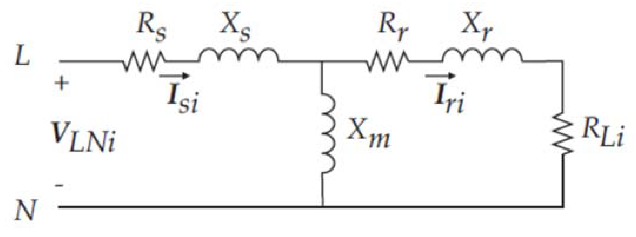
3.3. Model of the Electric Generator

The rated capacity of PRO power plants is expected to range from 5 kW to 5 MW, where the asynchronous (induction) generators are a suitable option for electric power generation due to their lower cost compared to other generator technologies [10]. Accordingly, the asynchronous generator is considered here to transform into electric power the net mechanical power P_mech produced by the turbine from the pressure retarded osmosis mechanism. Furthermore, for the sake of simplicity but without loss of generality, it is considered the generator is directly connected to the distribution network through a coupling distribution transformer. Hence, the reactive power, voltage, and power factor controls can be neglected.

Bearing in mind these conditions, and that the PRO power unit is considered as a shunt element to perform the power flow study addressed in this work, at the k-th forward sweep step the assessment of the line currents ${\mathit{I}}_{abc}^{n_{PRO}}$ injected by the asynchronous generator at the connecting node n must be carried out. For this purpose, a model to assess those line currents ${\mathit{I}}_{abc}^{n_{PRO}}$ in terms of the known line-to-ground voltages ${\mathit{V}}_{abc}^n$ at the connecting node n and the turbine mechanical power P_mech is formulated below, based on the asynchronous generator model described in [21].

Figure 7 represents both the positive and the negative sequence line-to-neutral circuit models of the three-phase induction generator [21]. In this circuit model, V_LNi, I_si, R_s, and X_s represent the line-to-neutral phasor voltages, the line phasor currents, resistance, and reactance of the stator, respectively. Furthermore, X_m is the magnetization reactance, whereas I_ri, R_r, and X_r are the line phasor currents, resistance, and reactance of the rotor, respectively. The load resistance R_Li is used to represent the transformation of the mechanical power P_mech into active electric power $P_R$ in the rotor of the generator. The positive (resp. negative) sequence model is obtained by setting the value of the subscript i as 1 (resp. as 2) in these quantities.

The transformation of the mechanical power P_mech into the active electric power $P_R$ is formulated by the power balance Equation (57), where the sequence load resistances R_Li and the sequence rotor currents I_ri (for i = 1, 2) are given by (58) and (59), respectively. Note that these rotor currents depend on the stator currents I_si (for i = 1, 2), which are given by (60). In addition, the positive and negative sequence slips of the machine are represented by s_i (for i = 1, 2) in (58)–(60). The negative sequence slip s₂ can be expressed in terms of the positive sequence slip s₁, as denoted by (61). Lastly, the line-to-neutral phasor voltages V_LNi in (60) can be readily obtained from the known line-to-ground voltages ${\mathit{V}}_{abc}^n$ at the connecting node n according to (62), where ${\mathit{A}}_s{}^{-1}$ represents the inverse of the well-known symmetrical component transformation matrix. Thus, according to (58)–(62), in the non-linear power balance Equation (57) the single variable to be known is the positive sequence slip s₁. To obtain the value of s₁ from (57), the fsolve solver of MatLab^® for the solution of non-linear equations is used. For this purpose, an initial condition $s_1^0$ for s₁ must be assessed, as explained at the end of this section.

$$P_R+P_{mec}=(3{\left|{\mathit{I}}_{r1}\right|}^2{R}_{L1}+3 {\left|{\mathit{I}}_{r2}\right|}^2{R}_{L2})+P_{mech}=0$$

(57)

$$R_{Li}=\left(\frac{1-s_i}{s_i}\right)R_r; (\mathrm{for} i=1, 2)$$

(58)

$${\mathit{I}}_{ri}=\frac{j{X}_m}{j\left(X_r+X_m\right)+\raisebox{1ex}{$R_r$}\!\left/ \!\raisebox{-1ex}{$s_i$}\right.}{\mathit{I}}_{si}; (\mathrm{for} i=1, 2)$$

(59)

$${\mathit{I}}_{si}=\frac{V_{LNi}\left[j\left(X_r+X_m\right)+\left(\frac{R_r}{s_i}\right)\right]}{j{X}_m\left(j{X}_r+\frac{R_r}{s_i}\right)+\left(R_s+j{X}_s\right)\left[j\left(X_r+X_m\right)+\left(\frac{R_r}{s_i}\right)\right]}; (\mathrm{for} i=1, 2)$$

(60)

$$s_2=2-s_1$$

(61)

$${\mathit{V}}_{LNi}={\mathit{A}}_s{}^{-1}{\mathit{V}}_{abc}^n; (\mathrm{for} i=1, 2)$$

(62)

Once s₁ is obtained from the solution of (57), the negative sequence slip s₂ must be obtained from (61). Based on the value of these slips, the positive and negative stator currents I_si (for i = 1, 2) can be directly evaluated from (60). Lastly, using the resulting sequence currents I_si, the line currents ${\mathit{I}}_{abc}^{n_{PRO}}$ injected by the asynchronous generator at the k-th forward sweep step can be expressed as in (63), where the value of the zero-sequence current I_s0 must be set as zero (i.e., I_s0 = 0). This completes the PRO power unit current injection model sought.

$${\mathit{I}}_{abc}^{n_{PRO}}={\mathit{A}}_s\left[\begin{array}{c}{\mathit{I}}_{s0}\\ {\mathit{I}}_{si}\end{array}\right]; (\mathrm{for} i=1, 2)$$

(63)

Based on the information mentioned above, the net complex three-phase power S_3ϕ generated by the PRO power unit is obtained from (64), where the superscript T denotes transposed vector.

$${\mathit{S}}_{3\varphi }=P_{3\varphi }+j{Q}_{3\varphi }={\left({\mathit{V}}_{abc}^n\right)}^T{\left({\mathit{I}}_{abc}^{n_{PRO}}\right)}^{*}=\left[\begin{array}{ccc}{\mathit{V}}_{an}^n& {\mathit{V}}_{an}^n& {\mathit{V}}_{an}^n\end{array}\right]\left[\begin{array}{c}{\left({\mathit{I}}_a^{n_{PRO}}\right)}^{*}\\ {\left({\mathit{I}}_b^{n_{PRO}}\right)}^{*}\\ {\left({\mathit{I}}_c^{n_{PRO}}\right)}^{*}\end{array}\right]$$

(64)

Lastly, the solution of the Equation (65) for the load resistance R_L1 must be first carried out to obtain the initial condition $s_1^0$ of the positive sequence slip s₁ required for solving (57). The coefficients of (65) are given by (66). The general guidelines to Formulates (65) and (66) are given in [19]. The solution of (65) for R_L1 is directly obtained from (67), which yields the values R_L1a and R_L1b. Evaluating (68) with the resulting values of R_L1a and R_L1b yields two possible initial conditions $s_{1a}^0$ and $s_{1b}^0$ for the positive sequence slip s₁. Since the induction machine is operated as generator, $s_{1a}^0$ and $s_{1b}^0$ must lower than zero. Thus, the largest of these values is considered as the initial condition $s_1^0$, as denoted by (69). This value can be readily used to solve the non-linear Equation (57).

$$A_{EG}{R}_{L1}^2+B_{EG}{R}_{L1 }+C_{EG}=0$$

(65)

$$A_{EG}=P_{mech }; B_{EG}=2P_{mech }\left(R_r+R_s\right)-V_{LN1}^2;$$

$$C_{EG}=P_{mech }{\left(X_s+X_r\right)}^2-V_{LN1}^2\left(R_r+R_s\right)+P_{mech}{\left(R_r+R_s\right)}^2$$

(66)

$$R_{L1a},R_{L1b}=\frac{-B_{EG}\pm \sqrt{B_{EG}^2-4A_{EG}{C}_{EG}}}{2A_{EG}}$$

(67)

$$s_{1a}^0,s_{1b}^0=R_r/\left(R_r+R_{L1k}\right); (\mathrm{for} ka, b)$$

(68)

$$s_{1 }^0=max\left\{s_{1a}^0, s_{1b}^0 \right\}$$

(69)

4. Forward-Backward Sweep Method for Power Flow Analysis

The FBS method reported in [21] is adopted to addresses the modelling of PRO power units into the power flow analysis of three-phase radial distribution networks. Fundamentally, the FBS method iteratively performs forward and backward steps, where the models reported in the previous section must be evaluated to assess the steady-state electrical performance of the distribution system.

In order to provide a comprehensive description of the FBS method, some fundamental preliminary issues are first provided, then detailed formulation of the forward and backward steps to perform the FBS method considering the integration of PRO power units is given.

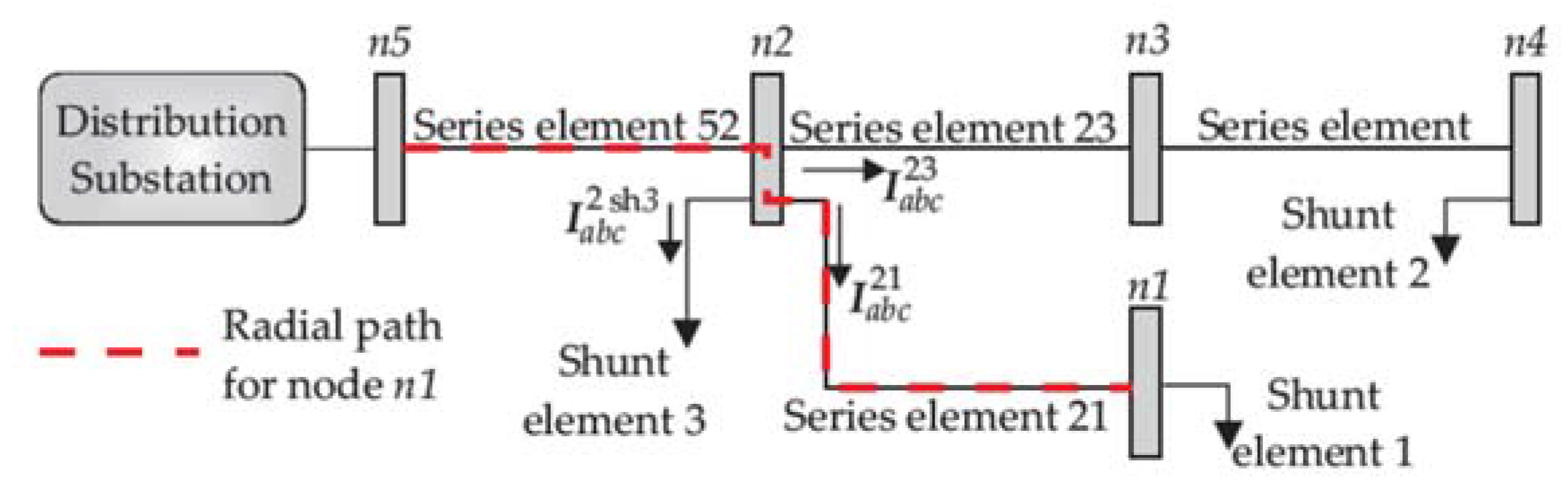
4.1. Preliminaries of the FBS Method

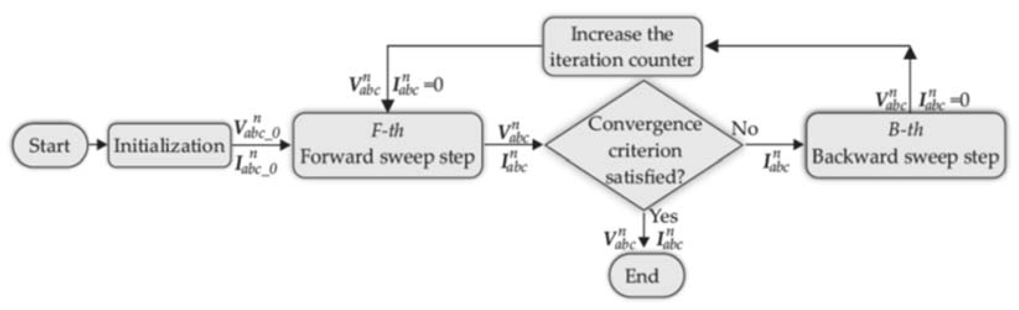
The FBS method can be applied to a radial system having n_b nodes, n_s serial components, and n_sh shunt components. The system has a distribution substation, with its terminal defined as the source node and denoted by n_f. Furthermore, the actual line-to-ground voltages are known from measurements and are denoted by ${\mathit{V}}_{abc}^{nf}$.

For the sake of illustration, the representative system shown in Figure 8 is considered where the node names are denoted as n1, n2, n3, n4, n5, whereas n_b = 5, n_s = 4, n_sh = 3, and n_f = n5.

To perform the forward and backward steps involved in the FBS method, the system’s nodes must be first sorted according to their depth levels in the distribution network. In the context of this work, the depth level Dp_n of a given node n is defined as the total number of series elements composing the radial path from that node to the source node n_f. Thus, the depth level of the given node n is straightforwardly evaluated by counting the serial components composing that radial path. For example, the system’s node n1 has a depth level Dp_n1 = 2 because its radial path is composed of two series elements, as shown in Figure 8. Note that the source node n_f is the only one with a depth level Dp_nf equal to 0. Once the depth levels Dp_n of all the system nodes are evaluated, the sorting is performed as follows. Let Sor be a set having n_b empty elements, thus having a cardinality of n_b. Then, assign to the first empty element of this set the name of the source node having the depth level equal to 0. In the following adjacent empty elements of Sor, assign the names of all the nodes having a depth level equal to 1, and so on until assigning in adjacent empty elements the names of all the remaining nodes according to their increasing depth levels. It is noted that the farthest node of the system can be defined as that node whose name is in the last element of Sor (i.e., Sor(n_b)). In this way, the nodes of the system have been sorted. For instance, in the sample system given in Figure 8, the nodes n1, n2, n3, n4, and n5 have depth levels of 2, 1, 2, 3, and 0, respectively. In this case, the Sor set is given by Sor = {n5, n2, n1, n3, n4}, where the name of the farthest node is n4 = Sor(5). It is pointed out that a computational routine can be implemented to readily assess the Sor set.

A complete forward sweep step goes over the nodes of the system in the order defined by Sor(n_FS) for n_FS = n_b, (n_b−1),…,1. On the contrary, a complete backward sweep step goes over the nodes of the system in the order defined by Sor(n_BS) for n_BS = 1, 2,…,n_b. In addition, when performing both the forward and backward sweep steps, the series and shunt elements connected to a given node n (n∈Sor) of depth level Dp_n and without any terminal connected to nodes of depth levels lower than Dp_n are called in this work as the downward elements connected to node n. It must be noted that the series downward elements connected to node n have their second terminal connected to different nodes of depth levels higher than Dp_n, such that these nodes are termed as child nodes of node n. The sum of the line currents transported by the downward elements connected to a given node n corresponds to the total line currents demanded at node n, and are denoted by ${\mathit{I}}_{abc}^n$. For instance, in the illustrative system shown in Figure 8, the downward elements connected to node n2 are given by the shunt element 3, the series element 23, and the series element 21. Hence the total line current demanded at node n2 is given by ${\mathit{I}}_{abc}^{n2}={\mathit{I}}_{abc}^{23}+{\mathit{I}}_{abc}^{21}+{\mathit{I}}_{abc}^{2 sh3}$. In addition, the child nodes of node n2 are n1 and n3.

To prepare the execution of the FBS method, the following must be realized. The node line-to-ground voltages ${\mathit{V}}_{abc}^n$ (for n = Sor(n_FS) and ∀n_FS = n_b, (n_b − 1), …, 1) are initialized in a balanced way according to the different voltage rating levels of the distribution system. In addition, the total line currents ${\mathit{I}}_{abc}^n$ for all nodes are initialized at zero. It is assumed that all the parameters of the line segments, transformer, and loads are already known.

In addition, before executing the FBS method, the mechanical power P_mech produced by the turbine must be evaluated from (56), which will be useful to compute from (63) the currents ${\mathit{I}}_{abc}^{n_{PRO}}$ injected by the PRO power unit along the entire iterative procedure. For this purpose, however, the known values of the salinity concentration C_r (resp. C_m) and the flow rate Q_r (resp. Q_m) of the river (resp. sea) water at the inlet of the membrane module must first be used to assess the spatial variations of the osmotic $\mathsf{\Delta }{\pi }_{pol}$ and the hydraulic $\mathsf{\Delta }{P}_h$ pressures (as explained in Section 3.1). The resulting values are used to evaluate the hydraulic power P_hyd from (51). Once P_hyd is computed, the turbine mechanical power P_mech is readily obtained from (56). It must be pointed out that the salinity gradient does not depend on the distribution system variables, hence the mechanical power P_mech remains constant to compute the currents injected by the PRO power unit along the entire procedure of the FBS method. However, note from (60) and (63) that the currents ${\mathit{I}}_{abc}^{n_{PRO}}$ injected by the PRO power unit do not remain constant, since they depend on the line-to-ground voltages at the node of connection. Lastly, it is assumed that all parameters involved in (27)–(60) are known.

4.2. The FBS Method

Suppose that the Sor set is known. In addition, consider that the line-to-ground voltages ${\mathit{V}}_{abc}^n$ and the total line currents ${\mathit{I}}_{abc}^n$ demanded for all the system nodes (i.e., for n = Sor(n_FS) and ∀n_FS = n_b, (n_b − 1),…,1) have been initialized, as previously explained in Section 4.1. Based on this information, the FBS method illustrated in Figure 9 is executed, as explained below. The method starts by performing a complete forward sweep step to update the values of ${\mathit{V}}_{abc}^n$ and ${\mathit{I}}_{abc}^n$ for all system nodes. Once this forward sweep step is completed, a given convergence criterion is verified. If this criterion is satisfied, the FBS method ends. Otherwise, a complete backward sweep step is executed to update only the values ${\mathit{V}}_{abc}^n$ for all nodes computed in the previous forward sweep step. Finally, a new complete forward sweep step is newly executed. This iterative process is repeated until the given convergence criterion is satisfied. At this end, the steady-state operating point of the system is known in terms of the values of ${\mathit{V}}_{abc}^n$ and ${\mathit{I}}_{abc}^n$. The iterative process shown in Figure 9 is detailed below.

The F-th forward sweep step starts at the farthest node n = Sor (n_b), and goes over the system nodes in the order n = Sor(n_FS) (for n_FS = n_b, (n_b − 1), …, 1) until reaching the source node n = Sor (1). When this F-th forward sweep step is going over a given node n = Sor(k∈n_FS), the forward sweep sub-step explained in Section 4.3 must be performed to update the values of the line-to-ground voltages ${\mathit{V}}_{abc}^n$ and the total line currents ${\mathit{I}}_{abc}^n$ demanded at that node. For this purpose, the forward sweep sub-step uses the models previously reported in Section 2 and the PRO power unit model included in Section 3. Thus, when the F-th forward sweep step is completed (i.e., the source node n = Sor (1) has been reached), the line-to-ground voltages ${\mathit{V}}_{abc}^n$ and the total line currents ${\mathit{I}}_{abc}^n$ demanded for all the system nodes have been updated.

Once the F-th forward sweep step is completed, the magnitudes of the line-to-ground voltages $\left|{\mathit{V}}_{abc}^n\right|$ resulting at the source node n = Sor (1) are compared to the magnitudes of the voltages $\left|{\mathit{V}}_{abc}^{nf}\right|$ known at that node. If the resulting maximum absolute error Emax is less than a specified tolerance (says 1 × 10⁻³), as denoted by (70), the FBS method ends. Otherwise, the line-to-ground voltages ${\mathit{V}}_{abc}^n$ estimated for the source node n = Sor (1) in the previous F-th forward sweep step are set as the known voltages ${\mathit{V}}_{abc}^{nf}$, as denoted by (71). The backward sweep step described below is then executed.

$$Emax=max\left|\left|{\mathit{V}}_{abc}^{\mathit{S}or \left(1\right)}\right|-\left|{\mathit{V}}_{abc}^{nf}\right|\right|\le Tol$$

(70)

$${\mathit{V}}_{abc}^{n=\mathit{S}or \left(1\right)}={\mathit{V}}_{abc}^{nf}$$

(71)

The B-th backward sweep step starts at source node n = Sor (1) and goes over the system nodes in the order n = Sor(n_BS) (for n_BS = 1, 2,…,n_b) until reaching the farthest node n = Sor (n_b). When this B-th forward sweep step is going over a given node n = Sor(k∈n_BS), the backward sweep sub-step explained in Section 4.4 must be performed in order to update the values of the line-to-ground voltages of the child nodes of node n. For this purpose, the backward sweep sub-step uses the models of the series components previously reported in Section 2. The PRO power unit and loads are classified as shunt elements; thus, they are not considered to perform the backward sweep sub-step. When the B-th backward sweep step is completed, the line-to-ground voltages ${\mathit{V}}_{abc}^n$ for all nodes have been updated. Lastly, the total line currents ${\mathit{I}}_{abc}^n$ computed for all nodes in the previous F-th forward sweep step are reset to a value of zero. The FBS method then returns to perform a new forward sweep step, by considering as the new initial condition the values of the line-to-ground voltages ${\mathit{V}}_{abc}^n$ updated in this latter B-th backward sweep step and the recently reset currents ${\mathit{I}}_{abc}^n$.

Once the convergence criterion given by (70) is satisfied, the line-to-ground voltages ${\mathit{V}}_{abc}^n$ and the total line currents ${\mathit{I}}_{abc}^n$ of all nodes are known, which implies that the line currents through all the system components are also known. This readily allows evaluating the power flows along the entire system, voltage drops, components overcurrent, etc., under the integration of PRO power units.

4.3. Forward Sweep Sub-Step

Let us suppose that the F-th forward sweep step is currently going over a given node n = Sor(k∈n_FS). Therefore, the actual values of the line-to-ground voltages ${\mathit{V}}_{abc}^n$ and the total line currents ${\mathit{I}}_{abc}^n$ demanded at node n are provided as initial conditions to perform the forward sweep sub-step formulated below.

Consider that $n_{Lin}^n$, $n_{Tran}^n$, $n_{Load}^n$, and $n_{PRO}^n$ are the number of distribution line segments, transformers, loads, and PRO power units, respectively, downward connected to node n. To update the line-to-ground voltages ${\mathit{V}}_{abc}^n$ and the total line currents ${\mathit{I}}_{abc}^n$ demanded at node n, the models (1)–(2), (4)–(5), (7), and (63) must be evaluated separately in the following sequence.

For each one of the $n_{Lin}^n$ line segments connected at node n the following evaluations are repeated. The j-th line segment has one terminal connected to node n; identify from the Sor set (or from the system diagram) the child node m at which the second terminal is connected. The present values of the line-to-ground voltages ${\mathit{V}}_{abc}^m$ and the total line currents ${\mathit{I}}_{abc}^m$ demanded at node m are already known. Then, these values together with the a, b, c, and d matrices for the j-th line segment connecting nodes n and m are used to evaluate the model given by (1) and (2). This evaluation yields a new value for the line-to-ground voltages ${\mathit{V}}_{abc}^n$ at node n, as well as the line currents ${\mathit{I}}_{abc}^{nm}$ flowing from node n to m through the j-th line segment. The line currents ${\mathit{I}}_{abc}^{nm}$ are used to update the present values of the total line currents ${\mathit{I}}_{abc}^n$ demanded at node n according to (70).

$${\mathit{I}}_{abc}^n={\mathit{I}}_{abc}^n+{\mathit{I}}_{abc}^{nm}$$

(72)

For each one of the $n_{Tran}^n$ transformers connected at node n, the following evaluations must be repeated. For the j-th transformer having a terminal connected at node n, a similar procedure as the previously mentioned for a line segment is carried out, but considering the a_t, b_t, c_t, and d_t matrices for the j-th transformer to evaluate (4) and (5), instead of (1) and (2).

For each one of the $n_{Load}^n$ loads connected at node n, repeat the following evaluations. For the j-th load, the present values of the line-to-ground voltages ${\mathit{V}}_{abc}^n$ at its connecting node n are already known. These values are used to evaluate the model (7) to obtain the line currents ${\mathit{I}}_{abc}^{n_{Load}}$ demanded at node n by the j-th load. The resulting line currents are used to update the present values of the total line currents ${\mathit{I}}_{abc}^n$ demanded at node n according to (73).

$${\mathit{I}}_{abc}^n={\mathit{I}}_{abc}^n+{\mathit{I}}_{abc}^{n_{Load}}$$

(73)

For each one of the $n_{PRO}^n$ PRO power units connected at node n, repeat the following evaluations. For the j-th PRO power unit, the present values of the line-to-ground voltages ${\mathit{V}}_{abc}^n$ at its connecting node n, as well as the turbine mechanical power P_mech, are already known. Based on these values, compute the positive sequence slip s₁ from (57) and then compute the sequence currents ${\mathit{I}}_{si}$ from (60). Lastly, evaluate the line currents ${\mathit{I}}_{abc}^{n_{PRO}}$ injected at node n by the j-th PRO power unit from (63), which are used to update the present values of the total line currents ${\mathit{I}}_{abc}^n$ demanded at node n according to (74).

$${\mathit{I}}_{abc}^n={\mathit{I}}_{abc}^n+{\mathit{I}}_{abc}^{n_{PRO}}$$

(74)

The evaluation of each series component provides a new value for the line-to-ground voltages ${\mathit{V}}_{abc}^n$ at node n. Note that the value of the voltages ${\mathit{V}}_{abc}^n$ obtained from the evaluation of the last series component is considered a result of the forward sweep sub-step. In addition, according to (72)–(74), the value of the total line currents ${\mathit{I}}_{abc}^n$ demanded at a node is given by the sum of the line currents transported by all the components downward connected to node n, which completes the results of the sub-step. It is pointed out that if $n_{Lin}^n=n_{Tran}^n=0$, only shunt components are connected to node n and the above procedures for series elements (line segments and transformers) must not be executed. In that case, the values of the voltages ${\mathit{V}}_{abc}^n$ at node n are not updated. An extreme case occurs when $n_{Lin}^n=n_{Tran}^n=n_{Load}^n=n_{PRO}^n$ = 0, implying the node n is on no load (open circuit) condition, thus none of the aforementioned procedures are executed and the values of both ${\mathit{V}}_{abc}^n$ and ${\mathit{I}}_{abc}^n$ are not updated.

4.4. Backward Sweep Sub-Step

Suppose the B-th backward sweep step is currently going over a given node n = Sor(k∈n_BS). Therefore, the actual line-to-ground voltages ${\mathit{V}}_{abc}^n$ at node n are provided to perform the backward sweep sub-step described below. It must be pointed out that if n = Sor(1), the values of ${\mathit{V}}_{abc}^n$ are those recently set according to (71). Otherwise, the values of ${\mathit{V}}_{abc}^n$ are given by those recently updated in the previous backward sweep sub-step executed in the present B-th forward sweep step.

Consider that $n_{Lin}^n$ and $n_{Tran}^n$ are the number of distribution line segments and transformers downward connected to node n, respectively. Recalling that shunt components are not involved in backward sweep step calculations, the line-to-ground voltages of the child nodes of node n can be updated by separately evaluating the models (3) and (6) in the following sequence.

For each one of the $n_{Lin}^n$ line segments connected at node n, repeat the following evaluations. The j-th line segment has one terminal connected to node n; identify from the Sor set (or from the system diagram) the child node m at which the second terminal is connected. The line currents ${\mathit{I}}_{abc}^{nm}$ flowing through the j-th line segment were computed at the previous F-th forward sweep step from (2) (see paragraph above (72)), and thus are known. The values of the line-to-ground voltages ${\mathit{V}}_{abc}^n$ and the line currents ${\mathit{I}}_{abc}^{nm}$ are used to evaluate the model (3) yielding the new value of the line-to-ground voltage ${\mathit{V}}_{abc}^m$ at the child node m.

For each one of the $n_{Tran}^n$ transformers connected at node n, repeat the following evaluations. The j-th transformer has one terminal connected to node n; identify from the Sor set (or from the system diagram) the child node m at which the second terminal is connected. The values of the line currents ${\mathit{I}}_{abc}^m$ at the secondary side of the transformer correspond to the total currents demanded at the child node m, which are obtained at the previous F-th forward sweep step and thus are known. Values of the line-to-ground voltages ${\mathit{V}}_{abc}^n$ and the line currents ${\mathit{I}}_{abc}^m$ are used to evaluate the model (6) and to obtain the new value of the line-to-ground voltage ${\mathit{V}}_{abc}^m$ at the child node m.

It must be noted that, according to the procedures mentioned above, the backward sweep sub-step allows updating the line-to-ground voltages of all the child nodes of a given node n at once. Lastly, an extreme case occurs when $n_{Lin}^n=n_{Tran}^n=0$, meaning that the node n has no child nodes to be processed. In this case, the procedures explained above are not executed.

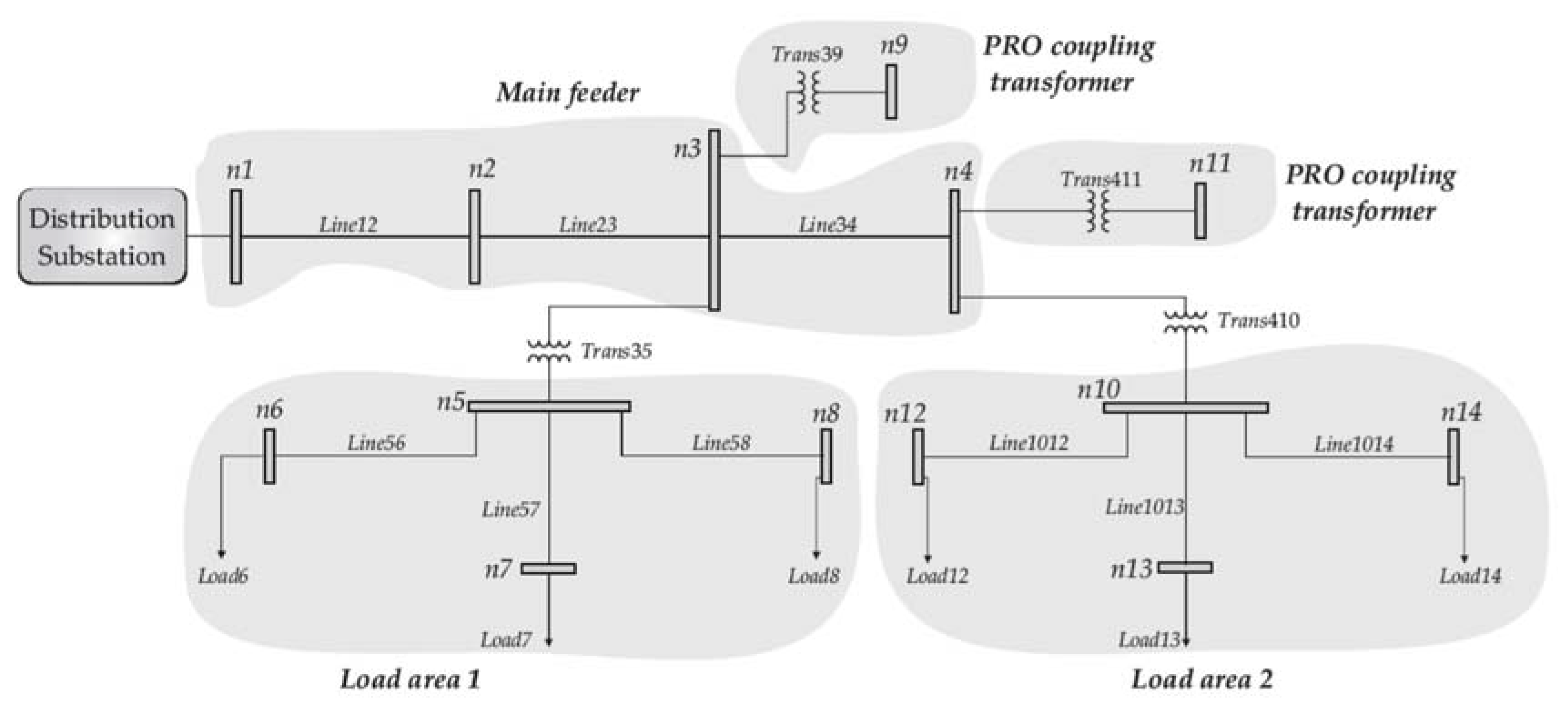
5. Numerical Results

The effectiveness of the proposed approach to estimating the steady-state operating condition of three-phase radial distribution networks under the integration of PRO power units is shown in this section through numerical results. For this purpose, the case study described below consists of power flow analysis of the 14 node distribution test system shown in Figure 10, considering the integration of PRO power units. Lastly, the nodes at which the PRO units were embedded are assumed to be those nearest to the coastline where the salinity gradient resource to produce electric power is located.

The general structure of the test system is organized into a distribution substation, a main feeder, two load supply areas, and two coupling transformer banks for the connection of PRO power units, as shown in Figure 10. The main feeder operates at a line-to-line voltage level of 4.16 kV and is connected to the secondary side of the distribution substation transformer. Load areas one and two as well as the secondary side of the PRO coupling transformers are at a line-to-line voltage level of 0.48 kV. This structure is composed of a total of nine distribution line segments, four transformers, and six loads. The distribution line segments of the main feeder are composed of three phase 1/0 AWG ACSR conductors. The secondary line segments in the load areas are composed of three phase and one neutral 1/0 AWG ACSR conductors. The PRO coupling transformers banks (Trans39 and Trans411) and the supply transformers (Trans35 and Trans410) are in delta-wye grounded connection with nominal power of 250 kVA and 100 kVA, respectively. All loads are in a balanced grounded wye connection and represented as constant complex powers, yielding a total three-phase power demand of 138 kW and 45 kVAR. The parameters of the system components are detailed in Appendix A.

The case study is developed in the following three parts. The first part consists of executing the FBS method to perform the power flow study for the base test system shown in Figure 10, i.e., without integration of PRO power units. The resulting steady-state base operating condition is discussed in Section 5.1. The second part executes the FBS method to perform the power flow study by considering two PRO power plants connected to nodes n9 and n11 of the system. Each power plant is composed of 25 PRO identical 7.5 kW units connected in parallel, resulting in a nominal power of 187.5 kW. The parameters of the power units are given in detail in Appendix A. Therefore, this second part of the case study yields the steady-state operating condition of the system under the integration of PRO power, which is presented in Section 5.2. Lastly, in Section 5.3, the operating conditions obtained in the first and the second part of the case study are additionally compared to reveal some effects on the steady-state performance of the system produced by the integration of the two PRO power plants.

For the first and second parts of the case study, the execution of the FBS method has been initialized as follows. The line-to-ground voltages ${\mathit{V}}_{abc}^n$ are initialized according to the values defined in (75) and (76), whereas the total line currents ${\mathit{I}}_{abc}^n$ are initialized at a value of zero, as denoted by (77). In addition, the source node is n1, i.e., n_f = n1, where the known line-to-ground voltages ${\mathit{V}}_{abc}^{nf}$ are given by (78). According to the depth levels of the system nodes, the Sor set is as given in (79). Lastly, the numerical results were obtained by using a computational program written in MatLab^® language, where the convergence tolerance Tol for the FBS method was set at a value of 1 × 10⁻³.

$${\mathit{V}}_{abc\text{\_}0}^n=2402{\left[\begin{array}{ccc}1\angle 0& 1\angle -120& 1\angle 120\end{array}\right]}^T, for \forall n=n1,n2, \dots , n4$$

(75)

$${\mathit{V}}_{abc\text{\_}0}^n=277{\left[\begin{array}{ccc}1\angle 0& 1\angle -120& 1\angle 120\end{array}\right]}^T, for \forall n=n5,n6, \dots ,n14$$

(76)

$${\mathit{I}}_{abc\text{\_}0}^n={\left[\begin{array}{ccc}0\angle 0& 0\angle 0& 0\angle 0\end{array}\right]}^T, for \forall n=n1,n2, \dots ,n14$$

(77)

$${\mathit{V}}_{abc}^{nf}=2402{\left[\begin{array}{ccc}1\angle 0& 1\angle -120& 1\angle 120\end{array}\right]}^T$$

(78)

$$\mathit{S}or=\left\{n1, n2, n3, n4, n5, n9, n6, n7, n8, n10, n11, n12, n13, n14\right\}$$

(79)

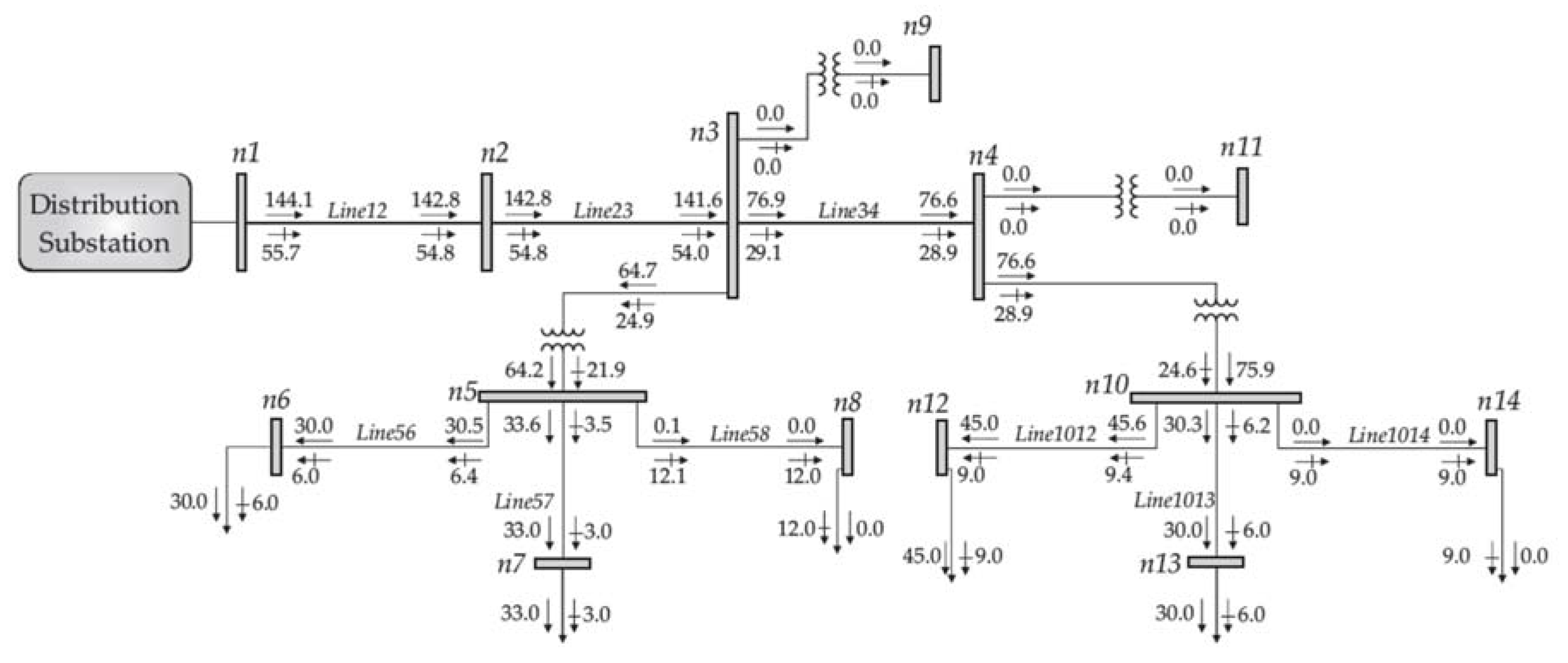
5.1. Steady-State Operating Condition for the Base Case

In this section, the steady-state operating condition of the base test system shown in Figure 10 obtained from the execution of the FBS method is presented. The execution of the method was initialized according to the conditions given by (75)–(79), and the tolerance convergence Tol = 1 × 10⁻³ was satisfied at the 4th iteration. The results obtained are discussed below.

On the one hand, the resulting magnitudes of the line-to-ground voltages of the system nodes are given in

Table 1. Line-to-ground nodal voltage magnitudes for the base case.

Node	Voltages (kV)
	${\mathit{V}}_{\mathit{a}\mathit{n}}$	${\mathit{V}}_{\mathit{b}\mathit{n}}$	${\mathit{V}}_{\mathit{c}\mathit{n}}$
n1	2.403	2.401	2.402
n2	2.379	2.380	2.378
n3	2.356	2.359	2.354
n4	2.343	2.347	2.342
n5	0.266	0.266	0.266
n6	0.261	0.262	0.261
n7	0.260	0.262	0.261
n8	0.265	0.265	0.265
n9	0.272	0.272	0.272
n10	0.263	0.264	0.264
n11	0.270	0.271	0.271
n12	0.259	0.261	0.260
n13	0.261	0.262	0.261
n14	0.263	0.263	0.263

. It is pointed out that along the main feeder the line-to-ground voltages decrease from the scheduled value of 2.402 kV (i.e., $4.16/\sqrt{3}$ kV) at the source node (n_f = n1) to those obtained for the node n4, as shown in rows 2 to 5 of Table 1. The voltage profile of the nodes in the main feeder, however, is acceptable, since the voltage drops do not exceed 5% of the nominal value of 2.402 kV. It must be noted, however, that the line-to-ground voltages levels of nodes n6, n7, n12, and n13 in the load supply areas present drops higher than 5% of the nominal value of 0.277 kV (i.e., $0.48/\sqrt{3}$ kV). Lastly, due to the balanced load conditions and the short length of the distribution line segments, the line-to-ground voltages of all the system nodes are almost balanced, as observed in Table 1.

The resulting magnitudes of the line currents flowing through all the series and shunt components of the system are shown in

Table 2. Component line current magnitudes for the base case.

Component	Node n	Node m	Current at Node n (A)			Current at Node m (A)
			${\mathit{I}}_{\mathit{a}}$	${\mathit{I}}_{\mathit{b}}$	${\mathit{I}}_{\mathit{c}}$	${\mathit{I}}_{\mathit{a}}$	${\mathit{I}}_{\mathit{b}}$	${\mathit{I}}_{\mathit{c}}$
Line12	n1	n2	21.4	21.4	21.4	21.4	21.4	21.4
Line23	n2	n3	21.4	21.4	21.4	21.4	21.4	21.4
Line34	n3	n4	11.6	11.6	11.6	11.6	11.6	11.6
Line56	n5	n6	39.1	39.0	39.1	39.1	39.0	39.1
Line57	n5	n7	42.4	42.2	42.3	42.4	42.2	42.3
Line58	n5	n8	15.1	15.1	15.1	15.1	15.1	15.1
Line1012	n10	n12	59.0	58.7	58.9	59.0	58.7	58.9
Line1013	n10	n13	39.1	39.0	39.0	39.1	39.0	39.0
Line1014	n10	n14	11.4	11.4	11.4	11.4	11.4	11.4
Trans39	n3	n9	0.0	0.0	0.0	0.0	0.0	0.0
Trans35	n3	n5	9.8	9.8	9.8	85.1	84.8	85.0
Trans411	n4	n11	0.0	0.0	0.0	0.0	0.0	0.0
Trans410	n4	n10	11.6	11.6	11.6	101.0	100.6	100.9
Load6	n6	-	39.1	39.0	39.1	-	-	-
Load7	n7	-	42.4	42.2	42.3	-	-	-
Load8	n8	-	15.1	15.1	15.1	-	-	-
Load12	n12	-	59.0	58.7	58.9	-	-	-
Load13	n13	-	39.1	39.0	39.0	-	-	-
Load14	n14	-	11.4	11.4	11.4	-	-	-

. It is observed that for each distribution line segment the corresponding line currents flowing into the terminal connected between nodes n and m have practically the same value, as seen in rows 2 to 10 of Table 2. This is because the shunt admittance for short distribution line segments is practically negligible. These results also confirm that line currents flowing through the line segments do not surpass the ampacity of the conductors (i.e., 230 A). Furthermore, note that for the base case the PRO coupling transformers Trans411 and Trans410 are on no-load condition; hence, their primary and secondary windings current equal 0A, since the magnetization current is neglected. Concerning the shunt components, the loads with higher line current are Load6, Load7, Load12, and Load13, which are connected to nodes n6, n7, n12, and n13, respectively (see rows 15 to 20 of Table 2). This is the reason these nodes present higher voltage drops with respect to their nominal value (see Table 1).

Lastly, by using the resulting line-to-ground voltages of the system nodes and the line currents, the three-phase complex power flow through the system components can be directly computed. For the analysis of the base case system, these power flows are given on the diagram shown in Figure 11. This diagram clearly shows that both active and reactive power flows are unidirectional, i.e., they are coming downstream in the system from the source node (distribution substation) to the load nodes in the load supply areas. In addition, the total three-phase complex power losses in the distribution network can be straightforwardly obtained from the power flows shown in Figure 11. In this case, the total three-phase complex power losses are 6.1 kW plus 10.7 kVAR. Adding these power losses and the total three-phase complex power load of the system (i.e., 138 kW and 45 kVAR), yields the total power supplied by the distribution substation 144.1 kW and 57.7 kVAR (see node n1 in Figure 11). This means that total power demand plus the distribution network losses are completely supplied by the distribution substation. These results show the characteristic steady-state behavior of traditional distribution systems without DG integration.

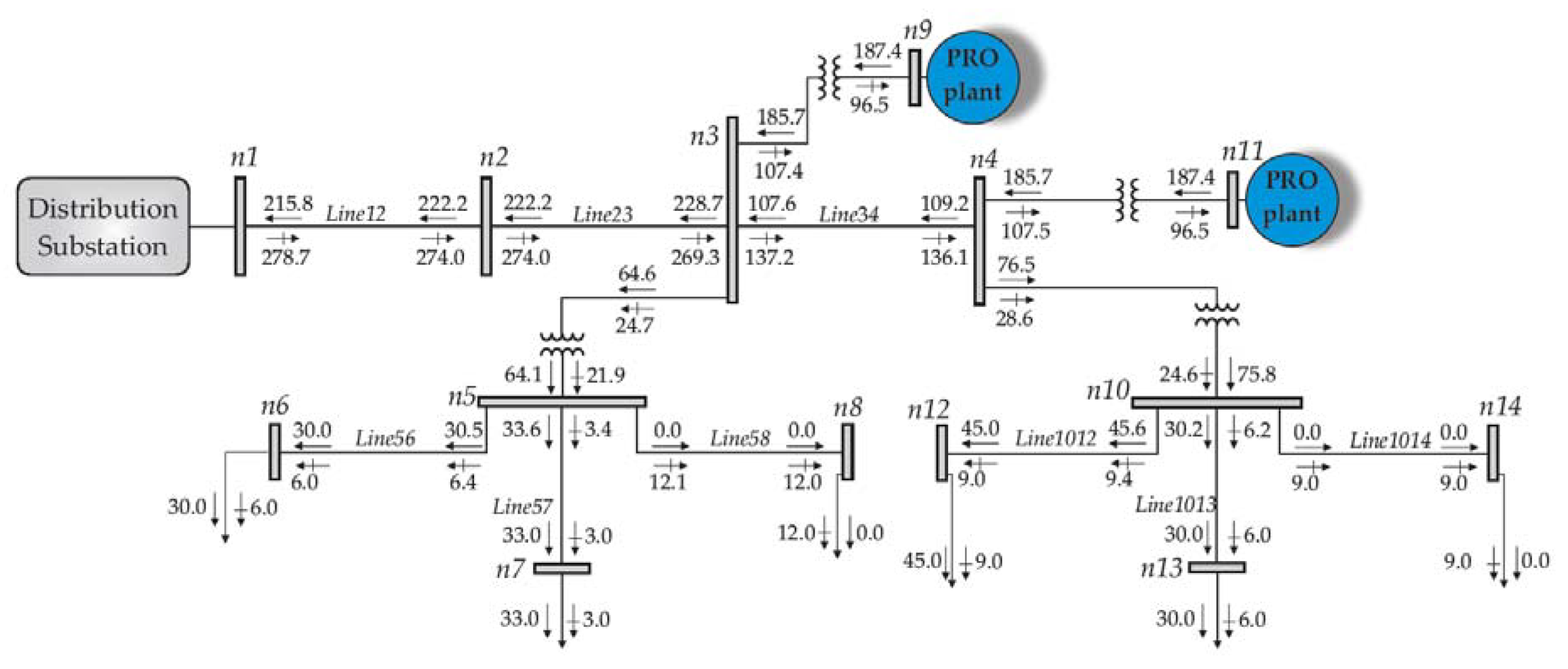
5.2. Steady-State Operating Conditions Considering the Integration of PRO Power Plants

In the second part of the case study, the power flow analysis of the 14 node test system is performed by the FBS method considering the integration of two PRO power plants; one connected to node 9 and the other connected to node 11, as shown below in Figure 12.

The initial values of the line-to-ground voltages, the total line currents for all the system nodes, the known voltage at the source node, and the Sor set are the same as those used in the base case. In addition, according to the preliminaries of the FBS method explained in Section 4.1, the mechanical power P_mech of each of the 50 PRO power units composing the two PRO power plants must be also assessed, which is performed as follows. Since the PRO power units are considered to have identical parameters and operating characteristics, it is only necessary to evaluate the mechanical power P_mech of a single PRO power unit from (56). To obtain P_mech, however, the hydraulic power P_hyd is firstly evaluated from (51), implying the solution of the polarization model (40)–(46) along with the evaluation of the spatial variation model (47)–(50) for the single PRO power unit. For this purpose, at the inlet of the membrane module of the single PRO power unit, the considered values of the salinity concentration C_r and C_m of the river and seawater were 0 g/L and 35 g/L, respectively, whereas the values of the flow rate Q_r and Q_m were set as 0.0012 m³/s and 0.0011 m³/s, respectively. Lastly, the parameters of the membrane module, the hydraulic system involved in (40)–(56), and the induction generator are given in Appendix A. According to these conditions, the mechanical power P_mech evaluated from (56) for a single PRO power unit is 7.49 kW.

The FBS method was executed and the convergence tolerance Tol = 1 × 10⁻³ was satisfied at the 4th iteration. It is important to point out that the number of iterations required to satisfy the convergence tolerance has not increased with respect to the base case. The resulting steady-state operating condition of the system under the integration of the PRO power plants is discussed below.

On the one hand, the resulting magnitudes of the line-to-ground voltages of all the system nodes are given in

Table 3. Line-to-ground nodal voltage magnitudes with PRO plants.

Node	Voltages (kV)
	${\mathit{V}}_{\mathit{a}\mathit{n}}$	${\mathit{V}}_{\mathit{b}\mathit{n}}$	${\mathit{V}}_{\mathit{c}\mathit{n}}$
n1	2.404	2.402	2.398
n2	2.407	2.402	2.400
n3	2.412	2.404	2.403
n4	2.414	2.404	2.403
n5	0.272	0.272	0.271
n6	0.267	0.268	0.266
n7	0.267	0.268	0.266
n8	0.271	0.271	0.270
n9	0.273	0.273	0.272
n10	0.272	0.272	0.270
n11	0.273	0.273	0.272
n12	0.268	0.268	0.267
n13	0.269	0.269	0.268
n14	0.271	0.271	0.270

. Due to the integration of the PRO power plants, the line-to-ground voltages along the main feeder now increases with respect to the nominal value of 2.402 kV scheduled at the source node (n_f = n1), as observed in rows 2 to 5 of this table. It must be pointed out, however, that the voltage profile along the main feeder is still acceptable because voltage raises do not exceed 5% of the nominal value of 2.402 kV. In addition, in the load supply areas, none of the line-to-ground nodal voltages exhibits a voltage drop higher than 5% of the nominal value of 0.277 kV, as shown in rows 6 to 15 of Table 3. Lastly, these results clearly show that, for the conditions considered in this case study, the nodal voltages remain almost balanced under the integration of the PRO power plants.

On the other hand, the line currents flowing through all the series and shunt components of the system are shown in

Table 4. Component line current magnitudes with PRO plants.

Component	Node n	Node m	Current at Node n (A)			Current at Node m (A)
			${\mathit{I}}_{\mathit{a}}$	${\mathit{I}}_{\mathit{b}}$	${\mathit{I}}_{\mathit{c}}$	${\mathit{I}}_{\mathit{a}}$	${\mathit{I}}_{\mathit{b}}$	${\mathit{I}}_{\mathit{c}}$
Line12	n1	n2	49.4	49.5	47.9	49.4	49.5	47.9
Line23	n2	n3	49.4	49.5	47.9	49.4	49.5	47.9
Line34	n3	n4	24.4	24.5	23.6	24.4	24.5	23.6
Line56	n5	n6	38.2	38.1	38.3	38.2	38.1	38.3
Line57	n5	n7	41.4	41.2	41.5	41.4	41.2	41.5
Line58	n5	n8	14.8	14.8	14.8	14.8	14.8	14.8
Line1012	n10	n12	57.1	57.0	57.4	57.1	57.0	57.4
Line1013	n10	n13	37.9	37.9	38.1	37.9	37.9	38.1
Line1014	n10	n14	11.1	11.1	11.1	11.1	11.1	11.1
Trans39	n3	n9	29.8	30.1	29.3	254.3	261.3	257.1
Trans35	n3	n5	9.6	9.6	9.6	83.0	82.8	83.3
Trans411	n4	n11	29.8	30.2	29.2	253.4	262.2	257.0
Trans410	n4	n10	11.3	11.3	11.3	97.9	97.7	98.3
Load6	n6	-	38.2	38.1	38.3	-	-	-
Load7	n7	-	41.4	41.2	41.5	-	-	-
Load8	n8	-	14.8	14.8	14.8	-	-	-
Load12	n12	-	57.1	57.0	57.4	-	-	-
Load13	n13	-	37.9	37.9	38.1	-	-	-
Load14	n14	-	11.1	11.1	11.1	-	-	-
PRO plant 1	n9	-	254.3	261.3	257.1	-	-	-
PRO plant 2	n11	-	253.4	262.2	257.0	-	-	-

. The results show that integration of the PRO plants does not produce overload currents in the line segments making up the main feeder and the load supply areas, since the ampacity of the line segment conductors is 230 A. It can also be noted that the PRO power plants inject considerably high line currents into the secondary windings of the coupling transformers; however, these are naturally reduced to low values at the primary windings according to the transformers’ turn ratios, as observed in rows 11, 13, 21, and 22.

Figure 12 portrays the resulting three-phase complex power flow through the system components. Each PRO power plant is generating a total active power of 187.4 kW from the salinity gradient energy, while demanding a reactive power of 96.5 kVAR due to the induction generators, as noted in nodes n9 and n11. The complex power outputs of both PRO power plants are equal in this case because they are considered to have the same capacity, and salinity gradient conditions and structure, and thus the resulting line-to-ground voltages at their connecting nodes have the same value (please compare nodes n9 and n11 from Table 3).

In this case, the total active and reactive system power losses are 21 kW and 40.7 kVAR, respectively. Subtracting the active power losses (21 kW) and the total active power load of the system (138 kW) from the active power produced by the two PRO power plants (374.8 kW) results in excess active power generation of 215.8 kW supplied to the distribution substation, as illustrated in Figure 12. This means that the total active power demanded in the two load areas plus the active power losses are being entirely supplied by the PRO power plants from the blue energy harvested from the salinity gradient. Arguably, the excess DG represents the active power transferred from the distribution system to the sub-transmission or transmission system. Contrary to the characteristic steady-state behavior of traditional distribution systems, in this case the active power is flowing upstream in the system along the main feeder toward the distribution substation, i.e., the integration of the PRO power plants has reversed the active power flow along the main feeder.

The two PRO power plants, however, impose an additional reactive power demand of 193 kVAR, which added to the total reactive power demand (45 kVAR) and total losses (40.7 kVAR) yields the total reactive power of 278.7 kVAR provided by the distribution substation, as observed from Figure 12. To reduce this reactive power consumption, reactive power compensation may be installed at the terminals of the PRO power plants. The three-phase apparent power of each PRO power plant is 210.9 kVA, therefore the coupling transformers Trans9 and Trans411 are operating within their nominal rating power (250 kVA). Power supply transformers Trans 35 and Trans410 are also operating within their rating power limits.

The results obtained in this section clearly reveal that the integration of the two PRO power plants has not produced overload currents or voltage limit violations along the distribution system. Furthermore, these results show that the transformers and the PRO plants are operating within their power rating limits.

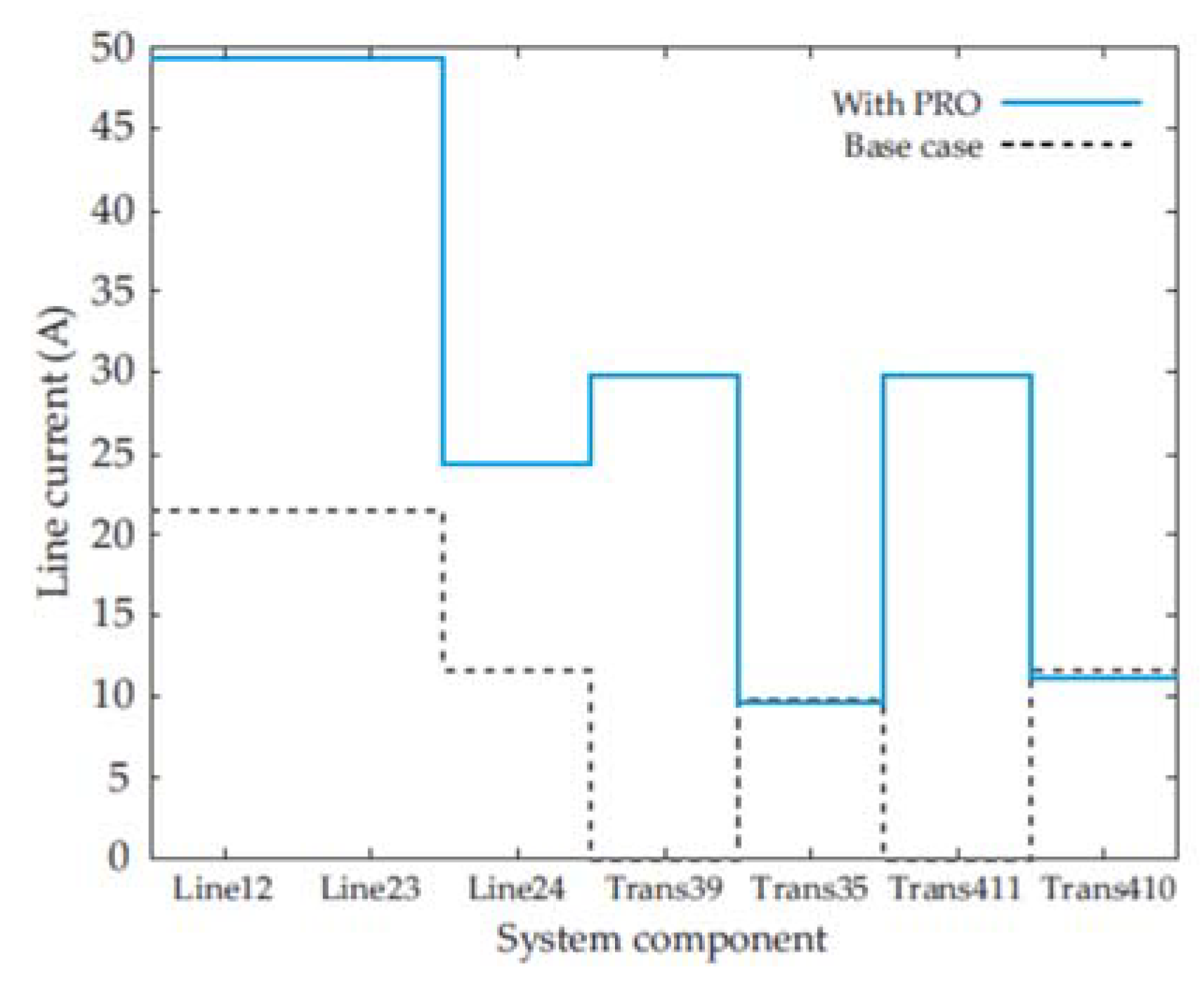
5.3. Comparison of the Steady-State Operating Conditions

The system operating conditions obtained with and without the integration of PRO power plants, as presented in Section 5.2 and Section 5.1, respectively, are compared in this section. This comparison allows evaluation of the effects on the steady-state performance of the system produced by integration of the two PRO power plants, as follows.

Figure 13 depicts the comparison of the line-to-ground voltage profiles for phase a of the system with and without the integration of PRO power plants. Since the nodal voltages are almost balanced in both cases (see Table 1 and Table 3), the voltage profile for phases b and c are omitted in this figure. In addition, the lower and upper voltage admissible limits are also illustrated. These limits were computed as a ±5% of the line-to-ground nominal voltage corresponding to the main feeder and the load areas, as illustrated in Figure 13a,b, respectively. This comparison clearly shows that the integration of the PRO power plants raises the nodal voltage profile of the overall system with respect to the base case, even though the electric generators composing these PRO plants are induction machines. In fact, it is observed in Figure 13b that some voltage lower limit violations in the load areas occur for the base case and are suppressed when the PRO power plants are connected.

In addition, Figure 14 illustrates the comparison of the line currents of some system components for the base case and for the case where the PRO plants are integrated. As in the voltage profiles shown in Figure 13, only the line currents corresponding to phase a are compared in this figure. Importantly, it is observed that the line currents increase in the line segments making up the main feeder when the PRO power plants are integrated into the system. For instance, the line current of the line segment Line12 increases by around 130% compared to the base case. Clearly, at the high voltage terminal of the coupling transformers Trans39 and Trans411, the line currents increase from zero to roughly 30 A due to the integration of the PRO power plants. In addition, at the high voltage terminal of the supply transformers Trans35 and Trans410 the line currents remain almost equal for both cases, meaning that the line currents in the load areas are not significantly affected by the integration of the PRO power plants.

Lastly,

Table 5. Effect of the integration of the PRO plants on the three-phase active and reactive power flow and system losses.

Description	Percentual Increment
Three-phase active power imported from the source node n1	−250%
Three-phase reactive power imported from the source node n1	400%
Three-phase active power total power losses	244%
Three-phase reactive power total power losses	339%

provides the percentual increments of the three-phase active and reactive power imported from the source node n1, as well as the active and reactive three-phase power total system losses driven by the PRO power plant integration with respect to the base case. This table reveals that the integration of the PRO power plants has importantly decreased (increased) the three-phase active (reactive) power imported from the source node n1. The active and reactive power losses, however, have substantially increased.

As concluding remarks for this case study, it must be pointed out that the integration of the two PRO power plants increases the voltage profile and the line currents along the main feeder. The resulting voltage profile and line currents, however, are still admissible for the system. Arguably, care must be taken because increasing the PRO power penetration level, reducing the total system load, and/or using a reactive power compensation scheme may steer the voltage profile and the line currents to surpass their admissible values. Concerns of this kind may be solved by the proposed approach.

6. Conclusions

This paper provides a comprehensive model for evaluating the electric current and power injected by a PRO power unit at its point of common coupling. The proposed model has been embedded within the FBS method in order to assess the steady-state condition of three-phase radial distribution systems under the integration of PRO power plants. Accordingly, this paper introduces the assembling of a novel model of PRO units for their direct inclusion in a power flow program for distribution systems. The prowess of the proposed approach has been shown through a numerical example. The results clearly show that the integration of PRO power plants drives increments in the main feeder voltage profile and line currents carried by components of the system, as well as reverse active power flows and low power factor at the source node. The results obtained are in agreement with common effects produced by the integration of DG into distribution systems.

The proposed approach could be used as a base to assess the limits of the penetration level of PRO power into distribution systems, which will be addressed in a forthcoming proposal. In addition, it is noteworthy that the consideration of different generator and coupling technologies as well as reactive power (power factor/voltage) control schemes in the proposed approach could be subjects of future research. Lastly, PRO power is a dispatchable renewable energy source, such that the inclusion of the proposed model in the optimal power flow problem of distribution grids may be relevant.

References

1. Mofor, L.; Goldsmith, J.; Jones, F. Ocean Energy: Techmology Readiness, Patents, Deployment Status and Outlook. 2014. Available online: https://www.irena.org/-/media/Files/IRENA/Agency/Publication/2014/IRENA_Ocean_Energy_report_2014.pdf (accessed on 21 August 2021).
2. Touati, K.; Tadeo, F.; Chae, S.H.; Kim, J.H.; Alvarez-Silva, O. Pressure Retarded Osmosis: Renewable Energy Generation and Recovery, 1st ed.; Academic Press: Cambridge, MA, USA, 2017; ISBN 978-0-12-812103-0. [Google Scholar]
3. Reyes-Mendoza, O.; Alvarez-Silva, O.; Chiappa-Carrara, X.; Enriquez, C. Variability of the thermohaline structure of a coastal hypersaline lagoon and the implications for salinity gradient energy harvesting. Sustain. Energy Technol. Assess. 2020, 38, 100645. [Google Scholar] [CrossRef]
4. Straub, A.P.; Deshmukh, A.; Elimelech, M. Pressure-retarded osmosis for power generation from salinity gradients: Is it viable? Energy Environ. Sci. 2016, 9, 31–48. [Google Scholar] [CrossRef]
5. Kempener, R.; Neumann, F. Salinity Gradient Energy Technology Brief. 2014. Available online: https://www.irena.org/-/media/Files/IRENA/Agency/Publication/2014/Jun/Salinity_Energy_v4_WEB.pdf (accessed on 21 August 2021).
6. Lee, C.; Chae, S.H.; Yang, E.; Kim, S.; Kim, J.H.; Kim, I.S. A comprehensive review of the feasibility of pressure retarded osmosis: Recent technological advances and industrial efforts towards commercialization. Desalination 2020, 491, 114501. [Google Scholar] [CrossRef]
7. Tran, T.T.D.; Bianchi, C.; Melville, J.; Park, K.K.; Smith, A.D. Design of housing and mesh spacer supports for salinity gradient hydroelectric power generation using pressure retarded osmosis. In Proceedings of the 2015 IEEE Conference on Technologies for Sustainability (SusTech), Ogden, UT, USA, 30 July–1 August 2015; pp. 141–147. [Google Scholar]
8. Kurihara, M.; Sakai, H.; Tanioka, A.; Tomioka, H. Role of pressure-retarded osmosis (PRO) in the mega-ton water project. Desalin. Water Treat. 2016, 57, 26518–26528. [Google Scholar] [CrossRef]
9. Matsuyama, K.; Makabe, R.; Ueyama, T.; Sakai, H.; Saito, K.; Okumura, T.; Hayashi, H.; Tanioka, A. Power generation system based on pressure retarded osmosis with a commercially-available hollow fiber PRO membrane module using seawater and freshwater. Desalination 2021, 499, 114805. [Google Scholar] [CrossRef]
10. Ackermann, T.; Andersson, G.; Söder, L. Distributed generation: A definition. Electr. Power Syst. Res. 2001, 57, 195–204. [Google Scholar] [CrossRef]
11. Shayani, R.A.; de Oliveira, M.A.G. Photovoltaic Generation Penetration Limits in Radial Distribution Systems. IEEE Trans. Power Syst. 2011, 26, 1625–1631. [Google Scholar] [CrossRef]
12. Jain, S.; Kalambe, S.; Agnihotri, G.; Mishra, A. Distributed generation deployment: State-of-the-art of distribution system planning in sustainable era. Renew. Sustain. Energy Rev. 2017, 77, 363–385. [Google Scholar] [CrossRef]
13. Hung, D.Q.; Mithulananthan, N.; Bansal, R.C. Analytical Expressions for DG Allocation in Primary Distribution Networks. IEEE Trans. Energy Convers. 2010, 25, 814–820. [Google Scholar] [CrossRef]
14. Fan, J.; Borlase, S. The evolution of distribution. IEEE Power Energy Mag. 2009, 7, 63–68. [Google Scholar] [CrossRef]
15. Alsafasfeh, Q.; Saraereh, O.; Khan, I.; Kim, S. Solar PV Grid Power Flow Analysis. Sustainability 2019, 11, 1744. [Google Scholar] [CrossRef] [Green Version]
16. Farag, H.E.; El-Saadany, E.F.; El Shatshat, R.; Zidan, A. A generalized power flow analysis for distribution systems with high penetration of distributed generation. Electr. Power Syst. Res. 2011, 81, 1499–1506. [Google Scholar] [CrossRef]
17. Kundur, P.; Paserba, J.; Ajjarapu, V.; Andersson, G.; Bose, A.; Canizares, C.; Hatziargyriou, N.; Hill, D.; Stankovic, A.; Taylor, C.; et al. Definition and classification of power system stability. IEEE Trans. Power Syst. 2004, 19, 1387–1401. [Google Scholar] [CrossRef]
18. Juarez, R.T.; Fuerte-Esquivel, C.R.; Espinosa-Juarez, E.; Sandoval, U. Steady-State Model of Grid-Connected Photovoltaic Generation for Power Flow Analysis. IEEE Trans. Power Syst. 2018, 33, 5727–5737. [Google Scholar] [CrossRef]
19. Llamas-Rivas, M.; Pizano-Martínez, A.; Fuerte-Esquivel, C.R.; Merchan-Villalba, L.R.; Gutiérrez-Martínez, V.J. Model for evaluating the electric power output of Pressure Retarded Osmosis generation plants. Int. Mar. Energy J. 2020, 3, 1–10. [Google Scholar] [CrossRef]
20. Naguib, M.F.; Maisonneuve, J.; Laflamme, C.B.; Pillay, P. Modeling pressure-retarded osmotic power in commercial length membranes. Renew. Energy 2015, 76, 619–627. [Google Scholar] [CrossRef]
21. Kersting, W.H. Distribution System Modeling and Analysis, 1st ed.; CRC Press: Boca Raton, FL, USA, 2001; ISBN 9780429125904. [Google Scholar]
22. Kersting, W.H. Distribution System Modeling and Analysis, 3rd ed.; CRC Press: Boca Raton, FL, USA, 2016; ISBN 9780429110443. [Google Scholar]
23. Maisonneuve, J.; Pillay, P.; Laflamme, C.B. Pressure-retarded osmotic power system model considering non-ideal effects. Renew. Energy 2015, 75, 416–424. [Google Scholar] [CrossRef]
24. IEEE Distribution System Analysis Subcommittee IEEE PES AMPS DSAS Test Feeder Working Group. Available online: https://0-site-ieee-org.brum.beds.ac.uk/pes-testfeeders/resources/ (accessed on 22 August 2021).
Figure 1. Distribution line segment (series component).
Energies 14 06649 g001
Figure 2. Shunt component.
Energies 14 06649 g002
Figure 3. Schematic representation of the PRO power unit.
Energies 14 06649 g003
Figure 4. Membrane module sketch.
Energies 14 06649 g004
Figure 5. Salinity polarization inside the membrane module.
Energies 14 06649 g005
Figure 6. Consecutive segments for a single spatial variation step evaluation.
Energies 14 06649 g006
Figure 7. Sequence line-to-neutral circuit model of the induction generator [21].
Energies 14 06649 g007
Figure 8. Representative radial distribution system.
Energies 14 06649 g008
Figure 9. Flowchart of the FBS method.
Energies 14 06649 g009
Figure 10. General structure of the test system.
Energies 14 06649 g010
Figure 11. Three-phase complex power flow diagram for the base case.
Energies 14 06649 g011
Figure 12. Three-phase complex power flow diagram for the base case.
Energies 14 06649 g012
Figure 13. Line-to-ground voltage profiles for (a) the main feeder and (b) the load areas and transformers.
Energies 14 06649 g013
Figure 14. Line currents for different system components.
Energies 14 06649 g014