Hybrid Protection Scheme Based Optimal Overcurrent Relay Coordination Strategy for RE Integrated Power Distribution Grid

Abstract

A directional overcurrent relay is commonly used to protect the power distribution networks of a distributed system. The selection of the appropriate settings for the relays is an important component of the protection strategies used to isolate the faulty parts of the system. The rapid growth of distributed generation (DG) systems present new challenges to these protection schemes. The effect of solar photovoltaic power plants on relay coordination is studied initially in this research work. A protection strategy was formulated to guarantee that the increased penetration of solar photovoltaic (PV) plants does not affect the relay coordination time. This paper addresses these issues associated with a high penetration of DG through the use of a hybrid protection scheme. The protection strategy is divided into two parts. The first part is based on an optimal fault current limiter value estimated with respect to constraints and the optimal time multiplier setting, and then the coordination time interval is estimated with respect to constraint in Part II. The results of these analyses show that a hybrid protection scheme can effectively handle the complexity of distributed generation (DG) and dynamic relay coordination problems. In this research, three optimization algorithms have been used for calculating the estimated value of impedance fault current limiter ($Z_{fcl}$) and time multiplier setting (TMS). The response time of hybrid protection schemes is very important. If the computational time of their proposed algorithms is less than their actual computational time, then their response time to address the issue is also less. The performance in all algorithms was identified to arrive at a conclusion that the grey wolf optimized algorithm (GWO) algorithm can substantially reduce the computational time needed to implement hybrid protection algorithms. The GWO algorithm takes a computational time of 0.946 s, achieving its feasible solution in less than 1 s.

1. Introduction

The directional overcurrent relay (DOCR) is an integral component of a mesh distribution network. It is used to ensure the effectiveness of the distribution network. Due to the increasing penetration of distributed generation (DG), modern power distribution systems need a new guided protection scheme [1,2,3].

The use of the DG unit increases the network’s short-circuit level, which could have a greater impact on the system. This is why the protection schemes are necessary to prevent these issues [4,5,6]. The main relay should be responsible for the clearing of the fault in a specified time. The backup protection device should also be designed to isolate the fault area in case of a failure of the primary relay [7,8]. This ensures that the continuity of power is maintained through the network’s healthy part. If a backup relay trip occurs before the main relay trip, it is called malfunctioning of the relay [9]. This type of tripping, also called the Sympathetic trip, are caused by the improper design of a protection scheme. They can be minimized by focusing on the most critical factors that affect their effectiveness [10]. The time multiplier and the pickup current are the two configurations that are commonly used in the design of DOCRs. The operation timeframe of these components depends on the relay type and the conditions under which it operates [11]. The ideal synchronization of the protection relays is a vital step in maintaining the system’s reliability. It involves finding the appropriate relay settings and ensuring that the backup relays are operating in coordination [12]. In other words, if the primary relay fails to take the necessary action, the backup relay will operate.

In the past years, various algorithms have been used to improve the coordination of relay systems. Some of these include the evolutionary algorithm, the metaheuristic algorithm, and the genetic algorithm, PSO, Gravitational search algorithm (GSA), GWO, Cuckoos and Firefly algorithm [13,14,15,16,17,18,19,20]. In [21], the authors presented an approach that is based on the predetermination of relay settings for different types of fault events. This is usually done through a graphical selection process [22].

In large power grids, the synchronization of relays and generators is a challenging problem. Usually, traditional techniques are used to reduce the total operating time of the relay [23]. However, these techniques are often not able to provide the results that are needed for complex problems [24,25]. The relay coordination problem is usually solved through a non-linear programming approach. Various techniques can improve the performance of the program such as heuristic optimization methods, genetic algorithms (GAs) [26], particle swarm optimization techniques [13], differential evolution algorithms (DEs) [27], and ant colony optimization [28]—but they are usually time-consuming [22,29,30]. The goal of this paper is to find an optimized relay coordination algorithm that can solve the relay coordination problem. It uses the concept of time relay multiplier setting and faults current limiter.

The three-optimization algorithms—GWO, GWO-PSO, and interior point algorithm—are used for determining the optimal performance of the hybrid protection scheme. Based on the performance of various optimization algorithms, it is decided which algorithm is better for the Hybrid Protection scheme.

The main contributions of this research article are as follows:

(1)

In modern times, renewable power has been massively integrated into the distribution grid, which has created a protection issue due to the rise of a heavy fault current;

(2)

This research paper presents a solution for the protection issue in the case of DGs penetration cases;

(3)

Identifying the main disadvantage of the traditional protection schemes is that they are unable to capture any changes in the system operation. This means that the selectivity calculations cannot be updated dynamically;

(4)

The hybrid protection scheme solves this issue in this research paper by introducing distributed generation protection monitoring index (DGPMI) in the protection scheme.

2. Modeling of Impedance Fault Current Limiter (Z_FCL) Based Optimal Relay Coordination Model (ORCM)

DOCRs are typically implemented in the distribution system. However, they are also very difficult to implement and reset as their dynamic changes are often very unpredictable. This means that they have dynamic changes that can affect the sensitivity and selectivity of the relays [12]. Due to the complexity of the task of implementing DOCRs, a new coordination algorithm is proposed to improve their reliability and sensitivity. This paper presents a new algorithm that can simultaneously update and verify the status of the system changes.

2.1. The Objective Function for Optimal Relay Coordination

The number of relays is represented as I, and relay operating time is depicted as t. K is the time taken by the relay to isolate the faulty section. In it, $w_i$ represents the weight factor of the operating relay. Here the value of the weight factor is taken as is in (1).

$$Min(k)={\displaystyle \sum _{i-1}^n{w}_i{t}_i}.$$

(1)

The coordination time interval (CTI) is a function of the relay’s time interval. The main aspect of CTI is that the connected relay system must operate properly and be coordinated properly. In Equation (2), $\mathsf{\Delta }t$ represent the coordination time interval (CTI). CTI is the difference between the operating time of primary relay ($t_p$) and backup relay $(t_b)$.

$$\Delta t=t_b-t_p,$$

(2)

where,

$\Delta t$ = CTI (coordination time interval)

$t_b$ = Backup relay operating time

$t_p$ = Primary relay operating time

The overcurrent relay operating time is computed in Equation (3). The time needed to evaluate the delay in the operation of an overcurrent relay depends on the time multiplier setting (TMS). In Equation (3) A, B, and $\alpha$ represent the relay constant that depends on the type of relay considered. Here, the inverse definite minimum time (IDMT) and the moderately inverse setting was taken for analysis.

Here, the value of A is 0.0515, B is 0.1140, and $\alpha$ is 0.02.

$$t=TMS(\frac{A}{M^{\alpha }-1}+B).$$

(3)

$t$ = Operating time interval of overcurrent relay

$A,B,\alpha$ = Relay constants

$M$ = Plug setting multiplier

$$M=\frac{I_{sc}}{I_{Pickup}}.$$

(4)

In Equation (4) $I_{SC}$ and $I_{pickup}$ represent the short circuit current and relay pick up current, respectively. The plug setting multiplier (M) is computed as the ratio of the relay pick up and short circuit current; the value of M varying between 0 to 1.

2.2. The Constraint for the Overcurrent Relay Coordination Model

In Equation (5), $t_b$ and $t_p$, the main relay and the backup relay operating time are the two components that operate during service. The value of CTI is computed as a function of the backup relay’s operating times and the primary relay’s operating time. Here, the CTI value is taken as 0.2 s.

$$t_b-t_p\ge CTI.$$

(5)

The $T_i^{Min}$ and $T_i^{Max}$ the maximum and the minimum operating time of a relay are respectively indicated in Equation (6). The value of $T_i^{Min}$ and j$T_i^{Max}$ is taken as 0 and 1 s, respectively [31,32]. The equation is defined as

$$T_i^{\min }\le T\le T_i^{Max}.$$

(6)

The $TM{S}_i^{Min}$ and $TM{S}_i^{Max}$, the maximum and the minimum time multiplier setting of a relay, are respectively indicated in Equation (7). The value of $TM{S}_i^{Min}$ and $TM{S}_i^{Max}$ is taken as 0 and 1.5 s, respectively. The relay setting was used as per the company standard of AREVA, P121.

$$TM{S}_i^{Min}\le TM{S}_i\le TM{S}_i^{Max}.$$

(7)

The minimum pickup current value of the relay is the value indicated $I_{set}^{Min}$ when the load current pass is initiated $I_{load}^{Max}$. In similar cases, the maximum pickup current setting should be less than the minimum value between the maximum available tap settings that the relay $I_{se{t}_i}^{Max}$ and fault current $I_{fault}^{Min}$ the value that passes through it.

$$Max(I_{load}^{Max}{I}_{set}^{Min})\le I_{se{t}_i}\le Min(I_{fault}^{Min}{I}_{se{t}_i}^{Max}).$$

(8)

The objective function for impedance fault current limiter ($Z_{fcl}$):

Equation (9) represents the objective function for the impedance fault current limiter $(Z_{fcl})$. Here, $w_j$ is the weight factor which is considered as one, $Z_j$ is represented as the impedance of $Z_{fcl}$.

$$Min(Z_{fcl})={\displaystyle \sum _{i=1}^n{w}_j{Z}_j}.$$

(9)

In ZFCL impedance optimization, we have

$${\displaystyle \sum _{j=1}^n{Z}_{fcl}^{Min}}\le {\displaystyle \sum Z}\le {\displaystyle \sum _{j=1}^n{Z}_{fcl}^{Max}}.$$

(10)

The implementation of an $Z_{fcl}$ affects the system’s impedance values. This issue will lead to system failure and decrease the efficiency of an operational network. Equation (10), $Z$ represents the fault current limiter (FCL) impedance value and ${\displaystyle \sum _{j=1}^n{Z}_{fcl}^{Min}}$ and ${\displaystyle \sum _{j=1}^n{Z}_{fcl}^{Max}}$ are the lower and upper values of FCL. Here, ${\displaystyle \sum _{j=1}^n{Z}_{fcl}^{Min}}$ the value is taken as 0 and the maximum value is 60 ohms. ${\displaystyle \sum _{j=1}^n{Z}_{fcl}^{Max}}$ is obtained as 2% of the total connected impedance in the network. If ${\displaystyle \sum _{j=1}^n{Z}_{fcl}^{Max}}$ goes beyond that, it affects the system performance.

2.3. Distributed Generation Protection Monitoring Index (DGPMI)

The distributed protection monitoring index (DGPMI) is a calculation that shows the impact of distributed generators on the power grid. It provides a simple and accurate way to measure the impact of these distributed generations on the relay coordination of the grid. Where $\Delta DG$ and $\Delta CTI$ depict the change in DG penetration level and change in coordination time interval, respectively. The positive value of DGPMI shows the requirement for change in the relay setting.

$$DGPMI=\frac{-\Delta DG}{\Delta CTI}.$$

(11)

3. Proposed Hybrid Protection Scheme

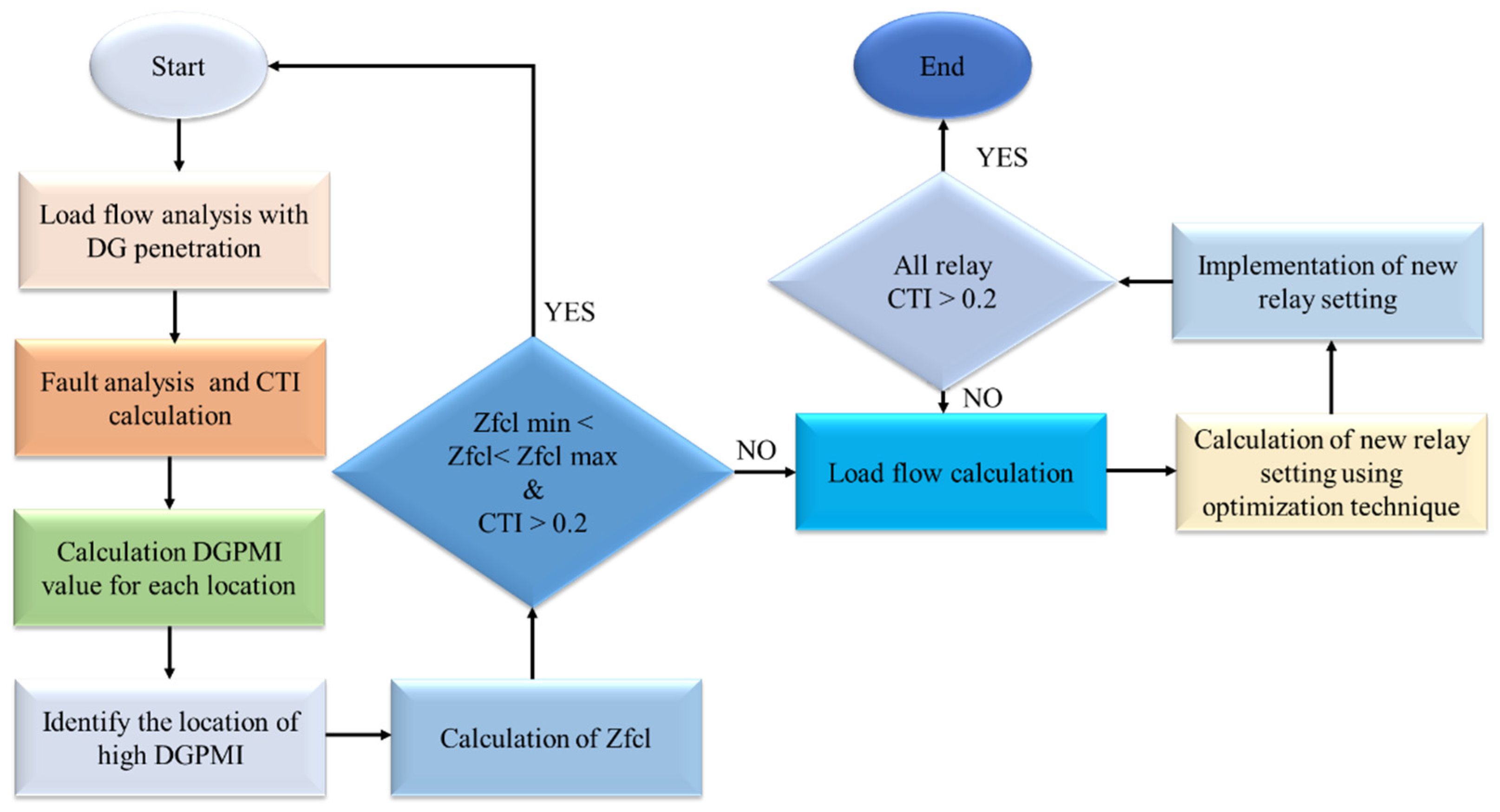
A hybrid protection algorithm combines the non-adaptive and adaptive algorithms (shown in Figure 1). It achieves higher reliability and flexibility. In Figure 1, Steps 1 to 7 of the algorithm refer to a non-adaptive protection scheme, while Steps 8 to 11 provide an adaptive protection scheme for hybrid protection. This hybrid protection scheme depicts the various measures that are needed to identify the optimum setting for minimizing $Z_{fcl}$ and TMS of the relay.

Various steps constituting the protection scheme algorithm are defined as under:

Step 1: Study the load flow for the entire network;

Step 2: Analyze the fault cases and the computed CTI;

Step 3: The DGPMI measures the effect of distributed generation (DGs) on the distribution grid;

Step 4: Identify the protected zones subjected to the penetration of generators;

Step 5: Determine the reactance value $Z_{\begin{array}{l}fcl\\ \end{array}}$ for the locations subjected to penetration by DGs.

In Equation (12), $X_{fcl}$ represents the reactance of $Z_{fcl}$, $I_{scA}$ represents the short circuit current after the $Z_{fcl}$ implementation, $I_{scB}$ represents the short circuit current before the $Z_{fcl}$ implementation.

$$X_{fcl}=\frac{V_{linetoline}}{\sqrt{3}}(\frac{1}{I_{scA}}-\frac{1}{I_{scB}}).$$

(12)

Equation (13) shows the calculation of impedance $Z_{fcl}$. Here, $R_{fcl}$ is taken as a variable that varies between 1 to 10. $X_{fcl}$ was calculated in Equation (12). The X/R value $Z_{fcl}$ is taken as a constant whose value varies between 0.1 to 5.

$$Z_{fcl}=\sqrt{R_{fcl}^2+X_{fcl}^2}.$$

(13)

Step 6: The total optimized $Z_{fcl}$ values for all parameters are measured within the defined maximum and minimum limits;

Step 7: If the $Z_{fcl}$ limits are not satisfied, then an algorithm resets the network for the load flow process;

Step 8: Calculation of optimized relay configurations;

Step 9: Setting the relay configuration for all relays;

Step 10: Checking the CTI of all relays and if coordination time interval (CTI) did not meet the limits, then steps 7 to 9 will be performed;

Step 11: Dynamic relay setting changes as per the DGs penetration level.

The optimal relay configuration can be achieved in two ways. First, decrease the fault current by using a fault current limiter. Then, dynamically change the relays settings. The goal of this test initially is to evaluate the performance of the IEEE 33 node network when connected to five solar PVs. Each photovoltaic (PV) power plant has a share maximum penetration level of 20% of load connected into the network.

In Figure 2, an IEEE 30 node feeder along with various PV-DGs connected to it is shown. The location of the relay and the Impedance fault current are indicated as R and Z.

List of Cases Considered to Analyze the Impact of Solar PV Penetration on the Power Distribution Grid

(1)

Case 1—0% penetration;

(2)

Case 2—20% penetration;

(3)

Case 3—40% penetration;

(4)

Case 4—60% penetration;

(5)

Case 5—80% penetration;

(6)

Case 6—100% penetration.

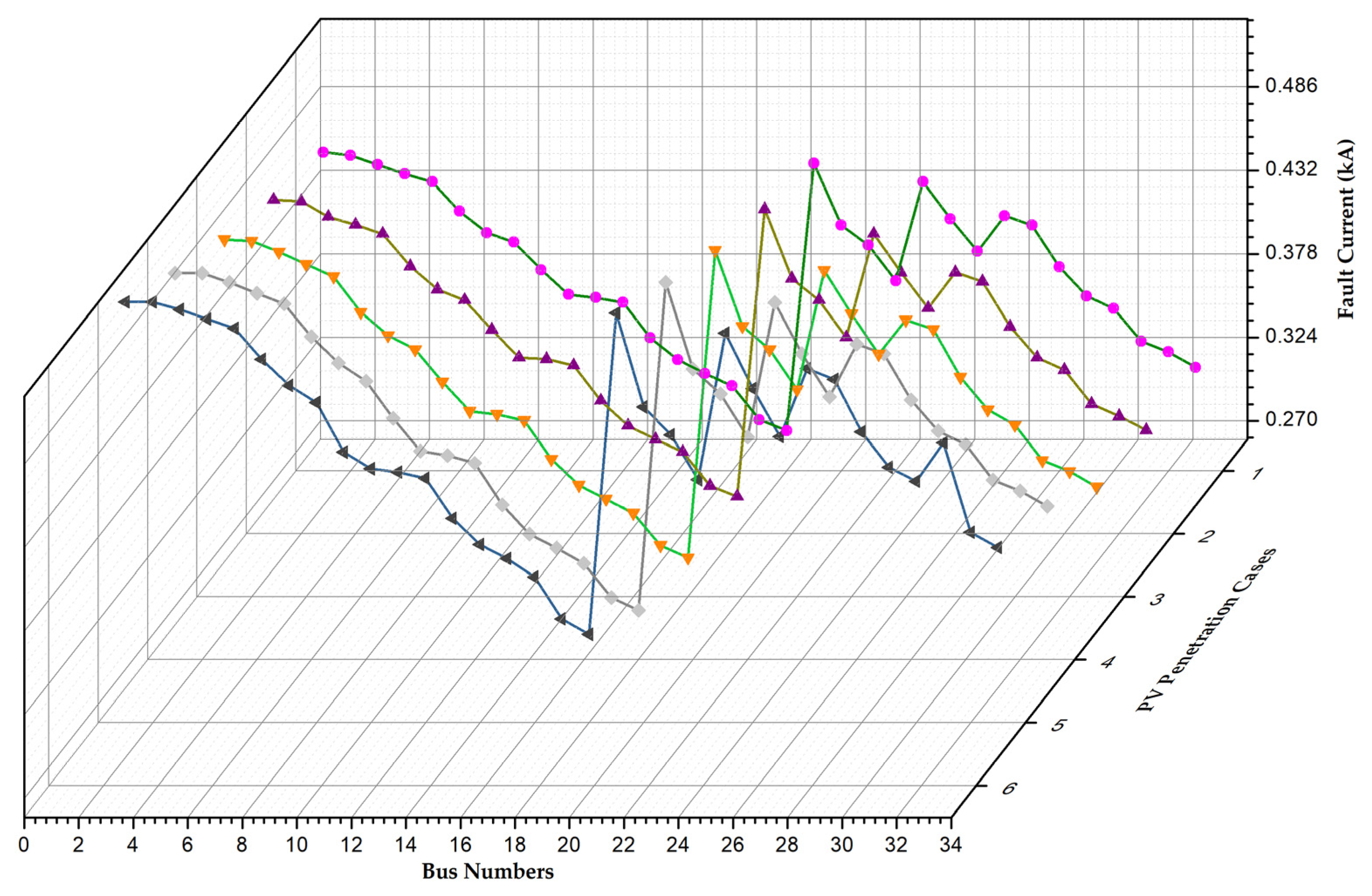
In Figure 3, the study revealed that the rise in fault current depends on the penetration level. It also noted that the maximum fault current rises when the penetration level reaches 100%.

The voltage variance of buses can be seen in Figure 4. It is also noted that the increasing solar PV penetration has improved the voltage profile of some buses. The study revealed that maximum voltage increases at 100% penetration level and the maximum voltage increase depends on the penetration level. The voltage variance was found as per the standard voltage variation limit, i.e., it is 2.5% [33].

4. Grey Wolf Optimization for Solving ORC

In 2014, Mirjalili [34] and colleagues proposed the framework for a grey wolf optimization algorithm known as GWO. It uses the concept of swarm intelligence to study the interactions between grey wolves and their packmates. The animals are organized into groups known as packages. The animal groups are classified as alpha, beta, delta, and omega. Alpha wolf (α) is based on the first rank of the public hierarchy, where it is considered the best expert and the other wolves in the wolf pack comply with its guidelines. Beta wolf (β) is the second level of management where the beta wolf supports the alpha for the tasks of the wolf pack. The third member of the public hierarchy is based on the delta (δ) wolves that follow the α as well as the β wolves. The rest of the wolves appear to be omega (ω). The GWO algorithm is organized into three stages: (1) looking, tracking, and approaching food, (2) circling and threatening food, and (3) assaulting food [34,35,36,37].

Grey wolves often surround their prey during the hunt. To study this behavior, the following equations are proposed.

$$D_1=C.X_{p1}(t)-X(t)$$

(14)

$$X(t+1)=X_{p1}(t)-A.D_1$$

(15)

Here, t represents the current iteration, $X_{p1}$ represents the vector position of food, and X indicates the vector position of the grey wolf. A and C are coefficient vectors. It can be determined by using the following equation:

$$A=2b-r_1-b$$

(16)

$$c=2r_2$$

(17)

Here, the value of b decreases linearly from two to zero through the entire iteration. The values of r₁ and r₂ are random numbers between 0 and 1. The location of food is known in the cycle of a hunting wolf. In the hunting process, the package is generated by α, β, and δ. The best-generated results are saved by the best agents and the remaining agents will update their positions. The selection of the best first, second, and third hunting agents can be rendered by using the following Equations (18)–(23):

$$D_{\alpha }=\left|C_1.X_{\alpha }-X\right|$$

(18)

$$D_{\beta }=\left|C_2.X_{\beta }-X\right|$$

(19)

$$D_{\delta }=\left|C_3.X_{\delta }-X\right|$$

(20)

$$X_1=X_{\alpha }+(A_1.D_{\alpha })$$

(21)

$$X_2=X_{\beta }+(A_2.D_{\beta })$$

(22)

$$X_3=X_{\delta }+(A_3.D_{\delta })$$

(23)

Reintroduce the position of the current hunting agent as shown in Equation (24).

$$X(t+1)=\frac{X_1+X_2+X_3}{3}$$

(24)

Grey wolves tend to finish the hunting process by attacking food. They attack correctly when food stops moving forward. It can be done mathematically by gradually lowering the value from 2 to 0. As a result, A is randomly modified with alpha variance and will be within the range [−1, 1], so the upcoming location of the search agents may be around its current position as well as around the position of the food. Grey wolves tend to finish the hunting cycle by consuming food.

5. Hybrid GWO-PSO for Solving ORC

In GWO-PSO, the position of the first three agents is updated in the search space by the proposed mathematical Equations (25)–(29). Instead of using the normal mathematical equations, the inertia constant for exploration and exploitation of the grey wolf in the search space is monitored. The updated set of governing equations are similar as in [38,39,40].

$$D_{\alpha }=\left|C_1.X_{\alpha }-w.X_1\right|$$

(25)

$$D_{\beta }=\left|C_2.X_{\beta }-w.X_2\right|$$

(26)

$$D_{\delta }=\left|C_3.X_{\delta }-w.X_3\right|$$

(27)

In the combination of GWO and PSO, the modified velocity and the updated equation are as follows.

$$V_i^{k+1}=w(V_i^k+(C_1\times ran{d}_1\times (pbes{t}_i-S_i^k))+(C_2\times ran{d}_2\times (gbes{t}_i-S_i^k))+(C_3\times ran{d}_3\times (gbes{t}_i-S_i^k)))$$

(28)

$$S_i^{k+1}=S_i^k+V_i^{k+1}$$

(29)

where $S_i^k$ and $S_i^{k+1}$ represent the previous and current position of “i” particle, $V_i^k$ and $V_i^{k+1}$ represent the previous and current velocity of “ith” particle, $pbest$ and $gbest$ are individual best positions and best global position found in the whole swarm. C₁ and C₂ are the acceleration constants, “$w$” is the inertia weight of PSO that lies between 0 and 1 and is defined as how much previous velocity is preserved. Each particle of PSO shares information with neighbours. The updated Equations (28) and (29) show that PSO associates each particle’s cognition component with the social component of the group. The social component advises that individuals overlook their own experience and alter their behavior according to the prior best particle in the neighborhood of the group.

In Equation (30), “$iter$” represents the rate of an ith individual at iteration. The weight factor varies iteratively in PSO.

$$w=(w_1-w_2)\times \frac{(\max it-iter)}{\max it}+w_2$$

(30)

where w₁ and w₂ represent first and last weight, respectively, matrix and iter show the largest current iteration number. Here, the value of w₁ and w₂ are taken as 0.9 and 0.4, respectively. The variable weight factor decreases the possibility of being trapped in local optima and also guides in scaling the optimal solution within a feasible range.

6. Interior Point Algorithm for Solving ORC Model

The MATLAB framework provides a very simple implementation of different non-linear optimization algorithms. Constraint mapping and problem definition are provided in a very user-friendly environment using the powerful ‘fmincon’ library function. The ‘fmincon’ function is used to find the minimum value of a function with respect to the constraints [41]. “fmincon” tries to solve the following problems:

$${}_x{}^{\min }f(x)s.t:A\ast X\le B,A_{eq}\ast X=B_{eq}$$

(31)

$$c(x)\le 0,C_{eq}(x)=0(Nonlinearconstraint)$$

(32)

$$LB\le x\le UB(Bonds)$$

(33)

The ‘fmincon’ function implements four different algorithms; (i) interior point (ii) sequential quadratic programming (SQP) (iii) active set, and (iv) trust reflective area. Any of those four algorithms can be selected by specifying the choice below:

$$option=optimset(‘Algorithm’,‘interiorpoint’).$$

(34)

The above options set are then passed to ‘fmincon’ for the implementation of the interior point algorithm. The following instructions, as Equation (35), are used to launch the optimization process.

$$x=f\min con(fun,x0,A,b,A_{eq},b_{eq},lb,ub,nonlcon,options).$$

(35)

7. Results and Discussion

Impedance Fault Current Limiter (Z_fcl) Optimization Using Grey Wolf Optimization

The Z, X, and R values are the most critical factors that determine the rising fault current. If the impedance is too high, it can cause the system operator to face system unbalanced issues while operating. In addition, if the X/R ratio is too high, it can cause the system operator to have the issue of grid parameter measurement.

The optimized value $Z_{fcl}$ is shown in

Table 1. Optimized $Z_{fcl}$ (ohms) parameters using the hybrid GWO-PSO algorithm.

Zfcl No.	Case 2			Case 3			Case 4			case 5			Case 6
	Z	R	X	Z	R	X	Z	R	X	Z	R	X	Z	R	X
1	0.50	0.10	0.49	0.84	0.16	0.82	1.32	0.26	1.30	1.89	0.37	1.85	2.50	0.49	2.45
2	0.25	0.05	0.24	0.62	0.12	0.61	1.11	0.22	1.09	1.71	0.34	1.68	2.32	0.46	2.27
3	0.37	0.07	0.36	0.61	0.12	0.60	1.22	0.24	1.19	1.86	0.37	1.83	2.52	0.49	2.47
4	0.38	0.07	0.37	0.67	0.13	0.65	1.18	0.23	1.16	1.88	0.37	1.85	2.58	0.51	2.53
5	0.58	0.12	0.57	0.84	0.17	0.83	1.31	0.26	1.28	2.06	0.40	2.02	2.81	0.55	2.75
6	0.51	0.10	0.50	0.71	0.14	0.70	1.14	0.22	1.12	2.04	0.40	2.00	2.89	0.57	2.83
7	0.59	0.12	0.58	0.76	0.15	0.75	1.23	0.24	1.20	2.12	0.42	2.08	3.02	0.59	2.96
8	0.70	0.14	0.69	0.84	0.17	0.82	1.23	0.24	1.21	2.05	0.40	2.01	3.03	0.60	2.98
9	0.83	0.16	0.81	0.93	0.18	0.91	1.26	0.25	1.24	2.03	0.40	1.99	2.82	0.55	2.77
10	1.02	0.20	1.00	1.02	0.20	1.00	1.34	0.26	1.31	2.09	0.41	2.05	3.39	0.67	3.33
11	1.03	0.20	1.01	1.08	0.21	1.06	1.35	0.27	1.33	2.06	0.41	2.02	3.43	0.67	3.36
12	1.11	0.22	1.09	1.11	0.22	1.09	1.38	0.27	1.36	2.06	0.40	2.02	3.50	0.69	3.43
13	1.41	0.28	1.38	1.41	0.28	1.38	1.60	0.31	1.57	2.26	0.44	2.21	3.97	0.78	3.89
14	1.77	0.35	1.74	1.63	0.32	1.60	1.77	0.35	1.74	2.37	0.47	2.33	4.38	0.86	4.29
15	1.88	0.37	1.84	1.74	0.34	1.70	1.88	0.37	1.84	2.51	0.49	2.46	4.62	0.91	4.53
16	2.07	0.41	2.03	1.91	0.38	1.88	1.99	0.39	1.95	2.59	0.51	2.54	4.71	0.92	4.61
17	2.41	0.47	2.36	2.23	0.44	2.19	2.41	0.47	2.36	3.01	0.59	2.95	5.09	1.00	4.99
18	2.65	0.52	2.59	2.46	0.48	2.41	2.55	0.50	2.50	3.19	0.63	3.13	5.23	1.03	5.13
19	0.25	0.05	0.25	0.64	0.13	0.63	1.10	0.22	1.08	1.72	0.34	1.68	2.31	0.45	2.27
20	0.17	0.03	0.17	0.43	0.08	0.42	0.83	0.16	0.82	1.34	0.26	1.31	1.91	0.38	1.88
21	0.14	0.03	0.14	0.36	0.07	0.36	0.76	0.15	0.74	1.25	0.25	1.23	1.80	0.35	1.77
22	0.10	0.02	0.10	0.31	0.06	0.30	0.65	0.13	0.64	1.13	0.22	1.10	1.71	0.34	1.67
23	0.31	0.06	0.30	0.57	0.11	0.56	1.16	0.23	1.14	1.81	0.36	1.78	2.44	0.48	2.39
24	0.21	0.04	0.21	0.46	0.09	0.45	1.02	0.20	1.00	1.57	0.31	1.54	2.19	0.43	2.15
25	0.14	0.03	0.14	0.33	0.06	0.32	0.81	0.16	0.80	1.36	0.27	1.33	1.95	0.38	1.91
26	0.56	0.11	0.55	0.72	0.14	0.71	1.12	0.22	1.10	2.05	0.40	2.01	2.88	0.56	2.82
27	0.48	0.10	0.48	0.65	0.13	0.64	1.07	0.21	1.04	2.01	0.40	1.97	2.83	0.56	2.78
28	0.45	0.09	0.44	0.55	0.11	0.54	0.93	0.18	0.91	2.07	0.41	2.03	2.85	0.56	2.80
29	0.33	0.07	0.32	0.38	0.08	0.38	0.75	0.15	0.74	2.06	0.40	2.02	2.80	0.55	2.75
30	0.29	0.06	0.28	0.34	0.07	0.34	0.62	0.12	0.61	2.05	0.40	2.01	2.82	0.55	2.76
31	0.32	0.06	0.32	0.32	0.06	0.32	0.58	0.11	0.56	2.19	0.43	2.15	5.14	1.01	5.04
32	0.27	0.05	0.26	0.20	0.04	0.20	0.53	0.10	0.52	2.21	0.43	2.17	2.96	0.58	2.90
∑	24.08	4.75	23.61	27.67	5.44	27.17	39.2	7.69	38.45	64.6	12.7	63.35	99.4	19.52	97.46

. It is the sum of the various parameters that are necessary to achieve the ideal relay coordination model. It shows the results of the experiments that were performed to determine the optimal relay coordination model. It is stated that the maximum value ${\displaystyle \sum }{Z}_{fcl}$ is 101.7281 ohms, which is higher than the limit of ${\displaystyle \sum }{Z}_{fcl}$ max (60 ohms).

The results of the hybrid GVO-PSO hybrid optimization are presented in

Table 2. Optimized $Z_{fcl}$ (ohms) parameters using the hybrid GWO algorithm.

Zfcl No.	Case 2			Case 3			Case 4			Case 5			Case 6
	Z	R	X	Z	R	X	Z	R	X	Z	R	X	Z	R	X
1	0.50	0.10	0.49	0.84	0.16	0.82	1.32	0.26	1.30	1.89	0.37	1.85	2.50	0.49	2.45
2	0.25	0.05	0.24	0.62	0.12	0.61	1.11	0.22	1.09	1.71	0.34	1.68	2.32	0.46	2.27
3	0.37	0.07	0.36	0.61	0.12	0.60	1.22	0.24	1.19	1.86	0.37	1.83	2.52	0.49	2.47
4	0.38	0.07	0.37	0.67	0.13	0.65	1.18	0.23	1.16	1.88	0.37	1.85	2.58	0.51	2.53
5	0.58	0.12	0.57	0.84	0.17	0.83	1.31	0.26	1.28	2.06	0.40	2.02	2.81	0.55	2.75
6	0.51	0.10	0.50	0.71	0.14	0.70	1.14	0.22	1.12	2.04	0.40	2.00	2.89	0.57	2.83
7	0.59	0.12	0.58	0.76	0.15	0.75	1.23	0.24	1.20	2.12	0.42	2.08	3.02	0.59	2.96
8	0.70	0.14	0.69	0.84	0.17	0.82	1.23	0.24	1.21	2.05	0.40	2.01	3.03	0.60	2.98
9	0.83	0.16	0.81	0.93	0.18	0.91	1.26	0.25	1.24	2.03	0.40	1.99	2.82	0.55	2.77
10	1.02	0.20	1.00	1.02	0.20	1.00	1.34	0.26	1.31	2.09	0.41	2.05	3.39	0.67	3.33
11	1.03	0.20	1.01	1.08	0.21	1.06	1.35	0.27	1.33	2.06	0.41	2.02	3.43	0.67	3.36
12	1.11	0.22	1.09	1.11	0.22	1.09	1.38	0.27	1.36	2.06	0.40	2.02	3.50	0.69	3.43
13	1.41	0.28	1.38	1.41	0.28	1.38	1.60	0.31	1.57	2.26	0.44	2.21	3.97	0.78	3.89
14	1.77	0.35	1.74	1.63	0.32	1.60	1.77	0.35	1.74	2.37	0.47	2.33	4.38	0.86	4.29
15	1.88	0.37	1.84	1.74	0.34	1.70	1.88	0.37	1.84	2.51	0.49	2.46	4.62	0.91	4.53
16	2.07	0.41	2.03	1.91	0.38	1.88	1.99	0.39	1.95	2.59	0.51	2.54	4.71	0.92	4.61
17	2.41	0.47	2.36	2.23	0.44	2.19	2.41	0.47	2.36	3.01	0.59	2.95	5.09	1.00	4.99
18	2.65	0.52	2.59	2.46	0.48	2.41	2.55	0.50	2.50	3.19	0.63	3.13	5.23	1.03	5.13
19	0.25	0.05	0.25	0.64	0.13	0.63	1.10	0.22	1.08	1.72	0.34	1.68	2.31	0.45	2.27
20	0.17	0.03	0.17	0.43	0.08	0.42	0.83	0.16	0.82	1.34	0.26	1.31	1.91	0.38	1.88
21	0.14	0.03	0.14	0.36	0.07	0.36	0.76	0.15	0.74	1.25	0.25	1.23	1.80	0.35	1.77
22	0.10	0.02	0.10	0.31	0.06	0.30	0.65	0.13	0.64	1.13	0.22	1.10	1.71	0.34	1.67
23	0.31	0.06	0.30	0.57	0.11	0.56	1.16	0.23	1.14	1.81	0.36	1.78	2.44	0.48	2.39
24	0.21	0.04	0.21	0.46	0.09	0.45	1.02	0.20	1.00	1.57	0.31	1.54	2.19	0.43	2.15
25	0.14	0.03	0.14	0.33	0.06	0.32	0.81	0.16	0.80	1.36	0.27	1.33	1.95	0.38	1.91
26	0.56	0.11	0.55	0.72	0.14	0.71	1.12	0.22	1.10	2.05	0.40	2.01	2.88	0.56	2.82
27	0.48	0.10	0.48	0.65	0.13	0.64	1.07	0.21	1.04	2.01	0.40	1.97	2.83	0.56	2.78
28	0.45	0.09	0.44	0.55	0.11	0.54	0.93	0.18	0.91	2.07	0.41	2.03	2.85	0.56	2.80
29	0.33	0.07	0.32	0.38	0.08	0.38	0.75	0.15	0.74	2.06	0.40	2.02	2.80	0.55	2.75
30	0.29	0.06	0.28	0.34	0.07	0.34	0.62	0.12	0.61	2.05	0.40	2.01	2.82	0.55	2.76
31	0.32	0.06	0.32	0.32	0.06	0.32	0.58	0.11	0.56	2.19	0.43	2.15	5.14	1.01	5.04
32	0.27	0.05	0.26	0.20	0.04	0.20	0.53	0.10	0.52	2.21	0.43	2.17	2.96	0.58	2.90
33	0.20	0.04	0.20	0.20	0.04	0.20	0.46	0.09	0.46	1.57	0.31	1.54	2.36	0.46	2.31
∑	24.08	4.75	23.61	27.67	5.44	27.17	39.2	7.69	38.45	64.6	12.7	63.35	99.4	19.52	97.46

. They show that the optimal relay coordination model was achieved with respect to constraints. The maximum value of ${\displaystyle \sum }{Z}_{fcl}$ shown is 101.7279 ohms. It was found that for cases 5 and 6, ${\displaystyle \sum }{Z}_{fcl}$ exceeds the maximum limit.

Figure 5 shows that the fault current rises at a certain level due to an increase in PV penetration. It is also shown that the optimized value $Z_{fcl}$ can limit the current under the given constraints. The figure shows the current level without $Z_{fcl}$ and with a $Z_{fcl}$. An analysis done on this graph shows that the optimized value $Z_{fcl}$ can limit the current under defined constraints.

Table 3. Relay TMS parameter optimization using the GWO algorithm for different cases.

Relay No.	TMS	TMS	TMS	TMS	TMS	TMS
	Case 1	Case 2	Case 3	Case 4	Case 5	Case 6
1	0.23604	0.2819	0.32488	0.36541	0.39683	0.41635
2	0.01102	0.0127	0.01293	0.01471	0.01619	0.01716
3	0.58011	0.65746	0.57655	0.67207	0.74049	0.77801
4	0.30318	0.34578	0.30424	0.35206	0.38749	0.40473
5	0.01445	0.01646	0.01643	0.0166	0.0184	0.01916
6	0.79849	0.92965	0.93176	0.93515	0.94198	0.97345
7	0.43132	0.50391	0.50466	0.50588	0.50824	0.49588
8	0.02161	0.02512	0.0256	0.02521	0.02532	0.02293
9	0.8951	1.03753	1.03736	1.04015	1.04498	0.91886
10	0.46694	0.53255	0.53266	0.53384	0.53721	0.46398
11	0.02258	0.02553	0.02553	0.0255	0.02575	0.0219
12	0.9613	1.02759	1.02771	1.02976	1.03768	0.85974
13	0.50123	0.51552	0.51538	0.51597	0.52012	0.42857
14	0.02565	0.02355	0.0236	0.02362	0.02376	0.01963
15	1.07091	0.93952	0.93803	0.9396	0.94686	0.97612
16	0.56537	0.46276	0.46203	0.46328	0.46696	0.48149
17	0.02832	0.02141	0.02137	0.02143	0.02164	0.02063
18	0.71013	0.53871	0.53755	0.53899	0.54308	0.5169
19	0.02309	0.02352	0.02398	0.024	0.0241	0.02445
20	0.57452	0.575	0.57578	0.57714	0.57891	0.52802
21	0.02907	0.02908	0.02911	0.02915	0.02922	0.02929
22	0.86045	0.86473	0.86763	1.00986	1.0159	1.02158
23	0.44724	0.44836	0.4499	0.45312	0.4565	0.46071
24	0.02441	0.02437	0.02443	0.0245	0.02475	0.02501
25	0.40761	0.41055	0.41155	0.41432	0.45464	0.45939
26	0.01963	0.01975	0.01981	0.01993	0.02178	0.02201
27	0.80199	0.80545	0.80657	0.81092	0.88658	0.88893
28	0.41143	0.41204	0.41249	0.4145	0.45154	0.45517
29	0.02027	0.02022	0.02023	0.0203	0.02184	0.02196
30	0.97795	0.97856	0.9783	0.97266	1.02856	1.05618
31	0.53539	0.53539	0.53513	0.53643	0.50387	0.50867
32	0.02972	0.02979	0.02967	0.02962	0.02232	0.02261

shows the optimized relay values that were obtained by GWO algorithms for running applications. These obtained values are used to maintain the necessary parameters of the overcurrent relay and the obtained results are capable of meeting all the practical constraints of the running network.

The optimized TMS values for the hybrid GWO-PSO algorithms and traditional interior-point algorithm are presented in

Table 4. Relay TMS parameter optimization using the hybrid GWO-PSO algorithm.

Relay	TMS	TMS	TMS	TMS	TMS	TMS
	Case 1	Case 2	Case 3	Case 4	Case 5	Case 6
1	0.23603	0.28196	0.32492	0.36541	0.39707	0.41655
2	0.01102	0.0127	0.01293	0.01476	0.01619	0.01716
3	0.57994	0.65707	0.5764	0.67776	0.74046	0.7807
4	0.30298	0.34557	0.30424	0.35241	0.38743	0.40492
5	0.01432	0.01635	0.01643	0.0166	0.01836	0.01916
6	0.79874	0.92913	0.93178	0.9351	0.94193	0.98603
7	0.43123	0.50379	0.50483	0.50571	0.50824	0.49652
8	0.02161	0.02512	0.02514	0.02519	0.02532	0.02288
9	0.89477	1.03753	1.03741	1.04053	1.04487	0.9207
10	0.46681	0.5326	0.53264	0.53399	0.53714	0.46411
11	0.02258	0.02545	0.02553	0.0255	0.02565	0.02186
12	0.96064	1.02736	1.02856	1.02971	1.03763	0.85965
13	0.50092	0.51545	0.51545	0.51577	0.52015	0.42846
14	0.02537	0.02355	0.02353	0.02358	0.02381	0.01961
15	1.07282	0.9417	0.93775	0.93946	0.94682	0.97531
16	0.5654	0.4651	0.46194	0.46312	0.467	0.48122
17	0.02832	0.02141	0.02137	0.02141	0.02158	0.02049
18	0.7101	0.53884	0.53762	0.53899	0.5434	0.51715
19	0.02309	0.02352	0.02398	0.02407	0.0241	0.02445
20	0.57452	0.575	0.57578	0.57714	0.57891	0.52802
21	0.02907	0.02908	0.02911	0.02915	0.02922	0.02929
22	0.86037	0.86401	0.86748	1.01001	1.01575	1.02166
23	0.44715	0.44826	0.44983	0.45318	0.45633	0.46041
24	0.02436	0.02437	0.02441	0.02455	0.02462	0.02476
25	0.40761	0.41055	0.41155	0.41432	0.45464	0.45939
26	0.01963	0.01975	0.01981	0.01993	0.02178	0.02201
27	0.80202	0.80754	0.80626	0.81078	0.88636	0.90285
28	0.41122	0.41297	0.41232	0.41445	0.45145	0.45848
29	0.02019	0.02022	0.02023	0.0203	0.02177	0.0224
30	0.97721	0.97921	0.97852	0.97283	1.02859	1.05569
31	0.53501	0.53547	0.53551	0.53669	0.50416	0.50846
32	0.02972	0.02967	0.02967	0.02962	0.02232	0.02254

and

Table 5. Relay TMS parameter optimization using the interior point algorithm.

Relay	TMS	TMS	TMS	TMS	TMS	TMS
	Case 1	Case 2	Case 3	Case 4	Case 5	Case 6
1	0.23598	0.28176	0.32487	0.36536	0.39678	0.41621
2	0.01102	0.0127	0.01293	0.01471	0.01619	0.01716
3	0.57991	0.65688	0.57638	0.67181	0.74044	0.77778
4	0.30298	0.3455	0.30424	0.35194	0.38743	0.40465
5	0.01432	0.01635	0.01643	0.0166	0.01836	0.01916
6	0.79814	0.92904	0.93094	0.93481	0.94191	0.97317
7	0.43113	0.50379	0.50406	0.50562	0.50824	0.49565
8	0.02161	0.02512	0.02514	0.02519	0.02532	0.02275
9	0.89473	1.03726	1.03726	1.03972	1.04465	0.91848
10	0.46678	0.53242	0.53264	0.53368	0.53704	0.46392
11	0.02258	0.02545	0.02553	0.0255	0.02565	0.02186
12	0.96057	1.02711	1.02711	1.02953	1.03755	0.85959
13	0.5009	0.51523	0.51523	0.51575	0.5201	0.42844
14	0.02537	0.02355	0.02353	0.02358	0.02376	0.01961
15	1.07049	0.93897	0.93773	0.93921	0.94663	0.97529
16	0.56532	0.46265	0.46192	0.46308	0.46687	0.48122
17	0.02832	0.02141	0.02137	0.02141	0.02158	0.02049
18	0.70995	0.53845	0.53753	0.53893	0.54301	0.51674
19	0.02309	0.02352	0.02398	0.024	0.0241	0.02445
20	0.57452	0.575	0.57578	0.57714	0.57891	0.52802
21	0.02907	0.02908	0.02911	0.02915	0.02922	0.02929
22	0.86035	0.86397	0.86748	1.00956	1.01568	1.02106
23	0.44715	0.44824	0.44983	0.4529	0.45633	0.46028
24	0.02436	0.02437	0.02441	0.0245	0.02462	0.02476
25	0.40761	0.41055	0.41155	0.41432	0.45464	0.45939
26	0.01963	0.01975	0.01981	0.01993	0.02178	0.02201
27	0.8014	0.80536	0.80616	0.81076	0.88632	0.88876
28	0.41088	0.41195	0.4123	0.41445	0.45145	0.45515
29	0.02019	0.02022	0.02023	0.0203	0.02177	0.02196
30	0.97716	0.97799	0.97799	0.97221	1.02816	1.05544
31	0.53498	0.53531	0.53508	0.53623	0.50375	0.50836
32	0.02972	0.02967	0.02967	0.02962	0.02232	0.02254

. These findings help in maintaining the proper coordination among the various components of a relay system. They also help in eliminating the possibility of a fault. These also indicate that the results of all tests are feasible and meet all defined constraints.

8. Results Validation

In Table 1 and Table 2, for all the optimized results, the $Z_{fcl}$ max limits are violated for cases 5 and 6. At this point, the hybrid protection algorithms start shifting towards the adaptive side. The validation part shows that the rise in fault current can lead to the malfunctioning of the relay. This also proves that the hybrid-protection scheme is capable of handling such a situation and overcoming the malfunctioning issue.

In the validation results in

Table 6. Validation of the hybrid protection scheme results.

Case No.	Fault Location	Relay		Before Setting Change			After Setting Change
		Primary Relay	Backup Relay	Tp	Tb	CTI	Tp	Tb	CTI
3	Bus 11	R10	R9	0.2011	0.3921	0.191	0.2018	0.4025	0.2007
4	Bus 11	R5	R4	0.1714	0.264	0.0926	0.3049	0.6193	0.3144
3	Bus 27	R26	R25	0.008	0.2071	0.1991	0.04	0.254	0.214
4	Bus 24	R23	R22	0.201	0.359	0.158	0.2061	0.4132	0.2071
6	Bus 11	R10	R9	0.2021	0.3921	0.19	0.2008	0.4025	0.2017
6	Bus 11	R5	R4	0.1724	0.264	0.14	0.3069	0.6193	0.3124
5	Bus 27	R26	R25	0.008	0.2061	0.1981	0.01	0.214	0.204
5	Bus 24	R23	R22	0.2024	0.3590	0.1566	0.2066	0.4232	0.2166

, cases 3 and 4 have been validated as relay settings obtained through the GWO and GWO-PSO, and can overcome malfunctioning through the use of non-adaptive protection as part of the hybrid protection scheme. The results before applying the hybrid protection scheme have violated the constraints. The main constraint, which is the CTI constraint, is satisfied after applying the hybrid protection scheme.

Similarly, for cases 5 and 6, the adaptive part of the hybrid protection scheme is applied because the max limit has been exceeded. After case 4, the hybrid protection schemes move toward the adaptive protection scheme, and it is found that the results are satisfied after applying the hybrid protection scheme with all constraints satisfied. All the obtained results prove that after the algorithms have been applied, the results are changed and satisfy all the constraints. It is found that the hybrid protection scheme is capable of handling every situation under the penetration cases considered.

The performance of the optimization algorithm is computed based on the time it takes to reach the feasible solution, as shown in

Table 7. Comparing computational time and iterations taken by an optimization algorithm for the non-adaptive part of the hybrid protection scheme.

Case No.	Fault Location	GWO		GWO-PSO
	Bus No.	Iteration	CPU Time (s)	Iteration	CPU Time (s)
3	10	20	0.956	5	1.032
4	5	19	0.936	6	1.056
3	26	17	0.947	6	1.078
4	23	21	0.993	7	1.098

. It is concluded that the GWO-PSOs algorithm performs better than the GWO algorithm iteratively and GWO performs better computational timewise.

In

Table 8. Comparing computational time and iterations taken by an optimization algorithm for the adaptive part of the hybrid protection scheme.

Case	Fault Location	Interior Point		GWO-PSO		GWO
	Bus No.	Iteration	CPU Time (s)	Iteration	CPU Time (s)	Iteration	CPU Time (s)
6	10	15	1.155	13	1.026	8	0.946
6	5	12	1.145	14	1.066	9	0.932
5	26	11	1.156	15	1.087	8	0.946
5	23	13	1.145	12	1.073	9	0.956

, the performance of the optimization algorithm is evaluated based on the time it takes to reach a feasible solution. It is concluded that the interior point algorithm performs better than the GWO and GWO-PSO algorithm iteratively and GWO performs better computational timewise.

Figure 6 shows that the hybrid approach of the GWO-PSO algorithms can provide feasible results in terms of constraints. In addition, it has been proven that the algorithm’s iterations can be decreased significantly. It has also been validated that the GWO algorithm takes less time to complete. The optimal solution time of the GWO algorithm is 0.956 s while the time required for the PSO algorithm is 1.03 s, as well as GWO, which takes 22 iterations and GWO-PSO, which takes 5 iterations to reach the feasible solution.

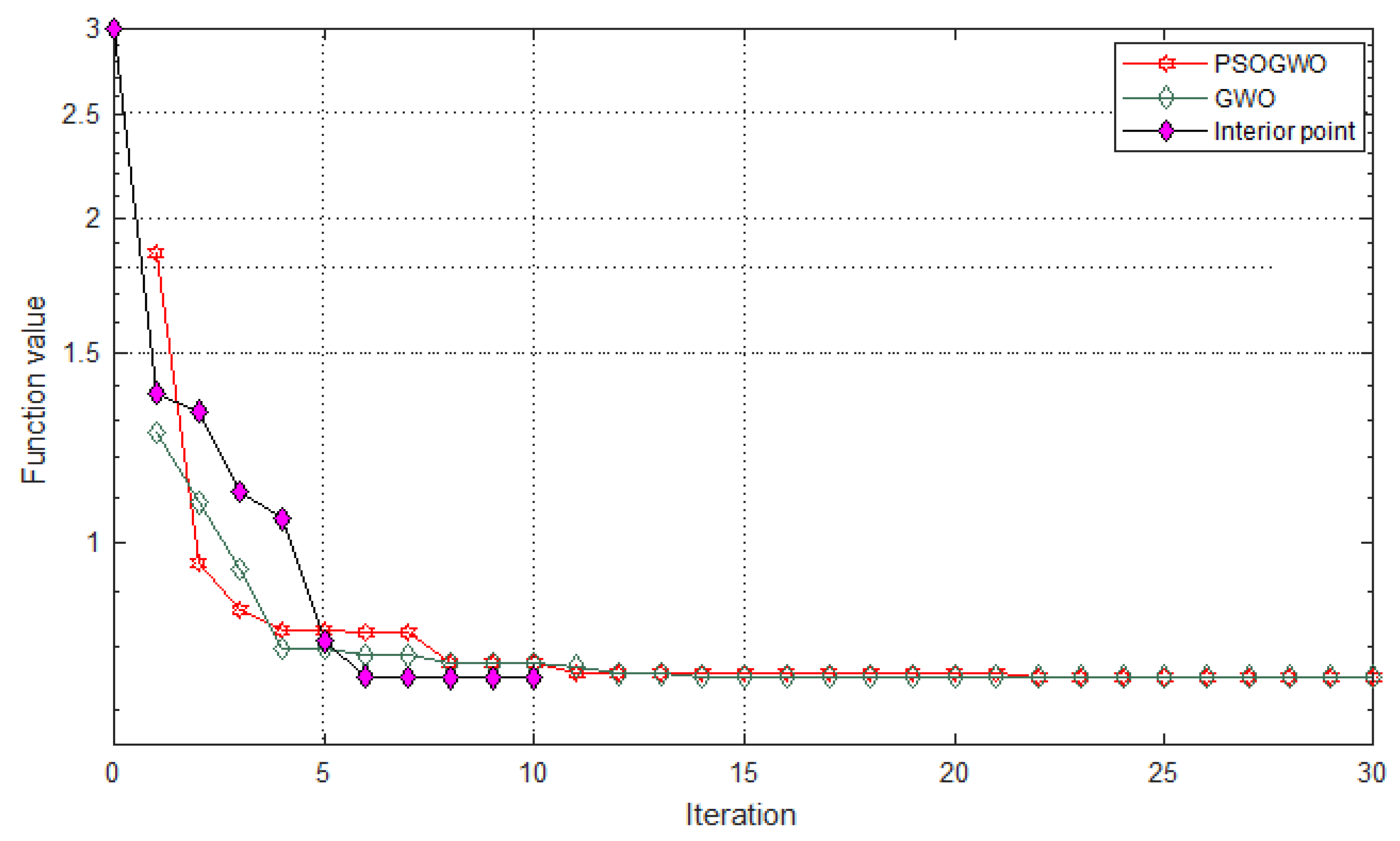
Figure 7 shows that the interior point, the hybrid approach of the GWO-PSO, and the GWO algorithms can provide feasible results in terms of the constraints for obtaining the TMS value of relay. In addition, it has been proven that the algorithm’s iterations can be decreased significantly. It has also been validated that the GWO algorithm takes less time to complete. The optimal solution computational time of the GWO algorithm is 0.946 s, while the computational time required for the GWO-PSO algorithm is 1.0266 s. The interior-point algorithm was taken at 1.155 s to reach the feasible solution with respect to constraints. The interior point algorithm takes 11 iterations, GWO takes 13 iterations, and GWO-PSO takes 14 iterations, respectively.

9. Statistical and Robustness Analysis

This section presents statistical evaluation methods that are based on the maximum, minimum, and standard deviation for the implemented algorithm and well-established algorithms existing in the literature. It also compares and contrasts the various algorithms in terms of precision and robustness.

The mean of the relay operational time is calculated to evaluate the accuracy of the implemented algorithm and the standard deviation is calculated to evaluate the dependability of the implemented algorithm.

Table 9. Statistical results for relay operational time for all the algorithms.

Algorithms	Minimum	Mean	Maximum	SD
GWO	9.258 × 10−2	1.258 × 10−3	9.048 × 10−1	1.354 × 10−4
GWOPSO	9.0551 × 10−1	3.150 × 10−2	9.060 × 10−1	1.270 × 10−2
Interior Point	9.6000 × 10−1	4.880 × 10−2	9.1697 × 10−1	1.620 × 10−2

displays statistical data for relay operational time.

In addition to normal statistical analysis, such as best, mean, worst, and standard deviation, the Friedman rank test is used to establish the significance of the data. This non-parametric test is also used to rate the algorithms for each investigated relay coordination model. The null hypothesis H0 (p-value greater than 5%) in the Friedman test indicates that there is no obvious difference between the compared methods. For all 30, the opposite hypothesis H1 indicates a significant difference between the compared methods. The Friedman rank test discovered that GWO algorithms rank first in this test, as shown in

Table 10. Friedman Ranking test of GWO and other well-established algorithms.

Algorithms	Friedman Ranking
GWO	1
GWOPSO	3
Interior Point	2

, indicating that the GWO algorithm produces more accurate results as compared with other algorithms.

10. Conclusions

In this research paper, the hybrid protection scheme is proposed for solving the relay coordination issue. This protection scheme is the hybrid version of the adaptive and non-adaptive protection scheme.

• The optimization algorithm is used to optimize the operational time of the hybrid protection scheme. The optimization algorithm used is GWO, GWO-PSO, and the interior point algorithm. These were used to solve the relay coordination problem.
• In the non-adaptive part of the hybrid protection scheme, GWO and GWO-PSO algorithms were used. In the adaptive part of the hybrid protection scheme interior point, GWO and GWO-PSO algorithms were used to solve relay coordination issue;
• All the tests were done on the IEEE 33 node feeder test. All the results found that a hybrid protection scheme is capable of handling any penetration case;
• In the protection scheme, a fast response is the most vital part. This response can be improved by optimization technique and the most important factor that plays an important role is the computational time;
• Among the proposed work optimization algorithms used for the hybrid protection scheme, the GWO algorithm takes the smallest computation time. The average computation time for GWO is 0.946 s;
• The conventional statistical analysis and Friedman ranking test illustrates that GWO outperforms as compared with other algorithms.

The results for the hybrid protection scheme revealed the effectiveness of the proposed strategy in establishing optimal relay settings by minimizing overall operation time while maintaining selectivity limitations across all protective devices.

References

- Sharma, A.; Dasgotra, A.; Tiwari, S.; Sharma, A.; Jately, V.; Azzopardi, B. Parameter Extraction of Photovoltaic Module Using Tunicate Swarm Algorithm. Electronics 2021, 10, 878. [Google Scholar] [CrossRef]
- Minciardi, R.; Robba, M. A Bilevel Approach for the Stochastic Optimal Operation of Interconnected Microgrids. IEEE Trans. Autom. Sci. Eng. 2017, 14, 1–12. [Google Scholar] [CrossRef]
- Kang, Q.; Zhou, M.; An, J.; Wu, Q. Swarm Intelligence Approaches to Optimal Power Flow Problem with Distributed Generator Failures in Power Networks. IEEE Trans. Autom. Sci. Eng. 2012, 10, 343–353. [Google Scholar] [CrossRef]
- Saldarriaga-Zuluaga, S.D.; López-Lezama, J.M.; Muñoz-Galeano, N. Optimal Coordination of Overcurrent Relays in Microgrids Considering a Non-Standard Characteristic. Energies 2020, 13, 922. [Google Scholar] [CrossRef] [Green Version]
- Huchel, L.; Zeineldin, H.H. Planning the Coordination of Directional Overcurrent Relays for Distribution Systems Considering DG. IEEE Trans. Smart Grid 2016, 7, 1642–1649. [Google Scholar] [CrossRef]
- Khodaei, A. Microgrid Optimal Scheduling with Multi-Period Islanding Constraints. IEEE Trans. Power Syst. 2013, 29, 1383–1392. [Google Scholar] [CrossRef]
- English, W.; Rogers, C. Automating relay coordination. IEEE Comput. Appl. Power 1994, 7, 22–25. [Google Scholar] [CrossRef]
- Wang, W.; Teh, K.C.; Li, K.H. Relay Selection for Secure Successive AF Relaying Networks with Untrusted Nodes. IEEE Trans. Inf. Forensics Secur. 2016, 11, 2466–2476. [Google Scholar] [CrossRef]
- Abidin, A.A.B.Z.; Ramasamy, A.K.; Nagi, F.H.; Abidin, I.Z. Determination of overcurrent time delay using fuzzy logic relays. In Proceedings of the 2009 Innovative Technologies in Intelligent Systems and Industrial Applications, Kuala Lumpur, Malaysia, 25–26 July 2009; IEEE: New York, NY, USA, 2009; pp. 480–485. [Google Scholar]
- Sharma, A.; Panigrahi, B.K. Interphase Fault Relaying Scheme to Mitigate Sympathetic Tripping in Meshed Distribution System. IEEE Trans. Ind. Appl. 2019, 55, 850–857. [Google Scholar] [CrossRef]
- ASadati, M.; Niassati, N.; Karegar, H.K. Improving Wind Turbines Protection by Shifting Pickup Current of Overcurrent Relay in Distribution Network. Available online:
https://www.infona.pl//resource/bwmeta1.element.ieee-art-000006254525 (accessed on 20 September 2020).
- Apostolov, A.P.; Tholomier, D.; Richards, S. Simplifying the configuration of multifunctional protection relays. In Proceedings of the 58th Annual Conference for Protective Relay Engineers, College Station, TX, USA, 5–7 April 2005 ; IEEE: New York, NY, USA, 2005; Volume 2005, pp. 281–286. [Google Scholar]
- Mansour, M.M.; Mekhamer, S.; El-Kharbawe, N. A Modified Particle Swarm Optimizer for the Coordination of Directional Overcurrent Relays. IEEE Trans. Power Deliv. 2007, 22, 1400–1410. [Google Scholar] [CrossRef]
- Tjahjono, A.; Anggriawan, D.O.; Faizin, A.K.; Priyadi, A.; Pujiantara, M.; Taufik, T.; Purnomo, M.H. Adaptive modified firefly algorithm for optimal coordination of overcurrent relays. IET Gener. Transm. Distrib. 2017, 11, 2575–2585. [Google Scholar] [CrossRef]
- Bayati, N.; Dadkhah, A.; Sadeghi, S.H.H.; Vahidi, B.; Milani, A.E. Considering variations of network topology in optimal relay coordination using time-current-voltage characteristic. In Proceedings of the 2017 IEEE International Conference on Environment and Electrical Engineering and 2017 IEEE Industrial and Commercial Power Systems Europe (EEEIC/I&CPS Europe), Milan, Italy, 6–9 June 2017; pp. 1–5. [Google Scholar] [CrossRef]
- Dehghanpour, E.; Karegar, H.K.; Kheirollahi, R.; Soleymani, T. Optimal Coordination of Directional Overcurrent Relays in Microgrids by Using Cuckoo-Linear Optimization Algorithm and Fault Current Limiter. IEEE Trans. Smart Grid 2016, 9, 1365–1375. [Google Scholar] [CrossRef]
- Al-Roomi, A.R.; El-Hawary, M.E. Optimal coordination of double primary directional overcurrent relays using a new combinational bbo/de algorithm. Can. J. Electr. Comput. Eng. 2019, 42, 135–147. [Google Scholar] [CrossRef]
- Shrivastava, A.; Tripathi, J.M.; Krishan, R.; Parida, S. Optimal Coordination of Overcurrent Relays using Gravitational Search Algorithm with DG Penetration. IEEE Trans. Ind. Appl. 2017, 54, 1. [Google Scholar] [CrossRef]
- Chabanloo, R.M.; Safari, M.; Roshanagh, R.G. Reducing the scenarios of network topology changes for adaptive coordination of overcurrent relays using hybrid GA–LP. IET Gener. Transm. Distrib. 2018, 12, 5879–5890. [Google Scholar] [CrossRef]
- Rajput, V.N.; Pandya, K.S.; Hong, J.; Geem, Z.W. A Novel Protection Scheme for Solar Photovoltaic Generator Connected Networks Using Hybrid Harmony Search Algorithm-Bollinger Bands Approach. Energies 2020, 13, 2439. [Google Scholar] [CrossRef]
- Singh, M.; Panigrahi, B.; Abhyankar, A. Optimal coordination of directional over-current relays using Teaching Learning-Based Optimization (TLBO) algorithm. Int. J. Electr. Power Energy Syst. 2013, 50, 33–41. [Google Scholar] [CrossRef]
- George, S.P.; Ashok, S. Forecast-based overcurrent relay coordination in wind farms. Int. J. Electr. Power Energy Syst. 2020, 118, 105834. [Google Scholar] [CrossRef]
- Razavi, F.; Abyaneh, H.A.; Al-Dabbagh, M.; Mohammadi, R.; Torkaman, H. A new comprehensive genetic algorithm method for optimal overcurrent relays coordination. Electr. Power Syst. Res. 2008, 78, 713–720. [Google Scholar] [CrossRef]
- Sachdev, M.S.; Ow, C.S.N. An on-line relay coordination algorithm for adaptive protection using line-ar programming technique. IEEE Trans. Power Deliv. 1996, 11, 165–173. [Google Scholar]
- Farzinfar, M.; Jazaeri, M.; Razavi, F. A new approach for optimal coordination of distance and directional over-current relays using multiple embedded crossover PSO. Int. J. Electr. Power Energy Syst. 2014, 61, 620–628. [Google Scholar] [CrossRef]
- Bedekar, P.P.; Bhide, S.R. Optimum coordination of overcurrent relay timing using continuous genetic algorithm. Expert Syst. Appl. 2011, 38, 11286–11292. [Google Scholar] [CrossRef]
- Shih, M.Y.; Enríquez, A.C.; Hsiao, T.-Y.; Treviño, L.M.T. Enhanced differential evolution algorithm for coordination of directional overcurrent relays. Electr. Power Syst. Res. 2017, 143, 365–375. [Google Scholar] [CrossRef]
- Shih, M.Y.; Salazar, C.A.C.; Enríquez, A.C. Adaptive directional overcurrent relay coordination using ant colony optimisation. IET Gener. Transm. Distrib. 2015, 9, 2040–2049. [Google Scholar] [CrossRef]
- Corrêa, R.; Cardoso, G.; Araujo, O.; Mariotto, L. Online coordination of directional overcurrent relays using binary integer programming. Electr. Power Syst. Res. 2015, 127, 118–125. [Google Scholar] [CrossRef]
- Alam, M.N.; Das, B.; Pant, V. An interior point method based protection coordination scheme for directional overcurrent relays in meshed networks. Int. J. Electr. Power Energy Syst. 2016, 81, 153–164. [Google Scholar] [CrossRef]
- Verma, R.K.; Singh, B.N.; Verma, S.S. Optimal Overcurrent Relay coordination Using GA, FFA, CSA Techniques and Comparison. IRJET J. 2017, 4, 928–932. [Google Scholar]
- Benabid, R.; Zellagui, M.; Chaghi, A.; Boudour, M. Application of Firefly Algorithm for Optimal Directional Overcurrent Relays Coordination in the Presence of IFCL. Int. J. Intell. Syst. Appl. 2014, 6, 44–53. [Google Scholar] [CrossRef] [Green Version]
- Mahmud, M.A.; Hossain, M.J.; Pota, H.R. Voltage Variation on Distribution Networks with Distributed Generation: Worst Case Scenario. IEEE Syst. J. 2014, 8, 1096–1103. [Google Scholar] [CrossRef]
- Pradhan, M.; Roy, P.; Pal, T. Oppositional based grey wolf optimization algorithm for economic dispatch problem of power system. Ain Shams Eng. J. 2018, 9, 2015–2025. [Google Scholar] [CrossRef]
- Jitkongchuen, D.; Phaidang, P.; Pongtawevirat, P. Grey wolf optimization algorithm with invasion-based migration operation. In Proceedings of the 2016 IEEE/ACIS 15th International Conference on Computer and Information Science (ICIS), Okayama, Japan, 26–29 June 2016; IEEE: New York, NY, USA, 2016; pp. 1–5. [Google Scholar]
- Amin, A.; Kamel, S.; Ebeed, M. Optimal reactive power dispatch considering SSSC using Grey Wolf algorithm. In Proceedings of the 2016 Eighteenth International Middle East Power Systems Conference (MEPCON), Cairo, Egypt, 27–29 December 2016; IEEE: New York, NY, USA, 2016; pp. 780–785. [Google Scholar]
- Korashy, A.; Kamel, S.; Jurado, F.; Youssef, A.-R. Hybrid Whale Optimization Algorithm and Grey Wolf Optimizer Algorithm for Optimal Coordination of Direction Overcurrent Relays. Electr. Power Compon. Syst. 2019, 47, 644–658. [Google Scholar] [CrossRef]
- Mirjalili, S.; Mirjalili, S.M.; Lewis, A. Grey Wolf Optimizer. Adv. Eng. Softw. 2014, 69, 46–61. [Google Scholar] [CrossRef] [Green Version]
- Pandi, V.R.; Zeineldin, H.H.; Xiao, W. Determining Optimal Location and Size of Distributed Generation Resources Considering Harmonic and Protection Coordination Limits. IEEE Trans. Power Syst. 2013, 28, 1245–1254. [Google Scholar] [CrossRef]
- Zeineldin, H.; El-Saadany, E.; Salama, M. Optimal coordination of overcurrent relays using a modified particle swarm optimization. Electr. Power Syst. Res. 2006, 76, 988–995. [Google Scholar] [CrossRef]
- Darvay, Z.; Rigó, P.R. New Interior-Point Algorithm for Symmetric Optimization Based on a Positive-Asymptotic Barrier Function. Numer. Funct. Anal. Optim. 2018, 39, 1705–1726. [Google Scholar] [CrossRef]