Energy Efficiency and Smooth Running of a Train on the Route While Approaching Another Train

Abstract

This paper presents an innovative technique of traffic management on a route divided into fixed block distances for trains equipped with a continuous area data transmission system that ensures information exchange between a train and a control center. The originality of the technique is focused on the optimization of the following train’s speed profile in terms of energy consumption under the need to maintain a minimum distance to the preceding train and to assume the smooth running of the following train, using elements of fixed and mobile block distance methods. The obtained results are an answer to the question of whether it is possible to obtain a smoother movement of the train and savings in mechanical energy consumption if the speed profile of this train is adjusted to the conditions before the train, such as information about the speed of the preceding train.

1. Introduction

The aim of this article is to analyze the possibility of reducing energy consumption during the procedure of approaching trains going in the same direction. An important aspect in the conducted research is the possibility of using data about the preceding train (speed) to regulate the running parameters of the following train. The use of such a solution leads to savings of mechanical energy and an increase in the smooth running of a train.

On the basis of the simulation, attempts were made to answer the question of what could be possible energy benefits from the speed equalization process between trains, as well as what problems may arise in this process.

Green rail is one of the slogans [1] which is currently guiding the research work carried out by the scientific teams of the railway industry, as well as the legislative work related to the new edition of the technical specification for interoperability relating to control-command and signaling [2]. One of the topics in the ecology of the railway system is energy efficiency in the movement of individual trains [3], and in the article [4] about Evaluation of Energy Efficiency Technologies for Rolling Stock and Train Operation of Railways (EVENT), the project contains information in the field of Energy Efficiency Technologies for Railways which is being collated, and present and future technologies are being evaluated for railway purposes.

One of the topics in the ecology of the railway system is energy efficiency in the movement of individual trains, which was presented in the publication [3]. On the other hand, the article [4] presents a project (EVENT), which includes the assessment of energy efficiency technology for rolling stock and rail train operation from the perspective of future railway needs.

The development of railway traffic control systems and area radio transmission systems (radio communication) [5], as far as data transmission between trains is concerned, opens new perspectives for solutions which have not been applied so far due to difficulties in technical implementation.

A great opportunity for this is seen in the work on new algorithms for automatic train control (ATC) [6] aimed at reducing energy consumption during runs. In the publication [7], the authors presented the optimization process results of switching points that initiate cruising and coasting phases of the driving. Due to nonlinear optimization formulation of the problem, nature-inspired evolutionary search methods, Genetic Simulated Annealing, Firefly, and Big Bang-Big Crunch algorithms were employed in this study. In [8], the authors presented a proposal for a mathematical model of Movement Authority in the ERTMS/ETCS system, which is an essential characteristic of the route for a train, and paper [9] presents proposals for the development of the ERTMS/ETCS system.

The benefits of improving the running of the train are achieved, among other things, as a result of selecting the appropriate parameters for determining the train braking curve in the ETCS system presented in [10] and on the basis of the proposed model based on Neural Networks for repetitive, defined phases and conditions of train running [11].

The idea of increasing smooth running is based on driving the train in a way that minimizes the need for speed changes (acceleration and braking). The risk of a train approaching the preceding train at a dangerous distance is one of the reasons for the need to brake or stop. On the other hand, one way to minimize this risk is to try to achieve a similar speed of both trains in order to maintain a constant distance between the trains, which can be assisted by exchanging information about the current operational speed.

A similar issue of movement was presented in the article [12]. This work presents an “operational” approach to the so-called coupling trains into convoys. The operational state, striving to couple trains, is a traffic situation analogous to the one analyzed in this article.

The proposed method implies train control using the ETCS L2 system, the functionality of which is complemented by additional functions. This additional function is the transmission of information to the following train about the movement parameters of the preceding train. The current specifications [13] do not foresee this possibility, but RBC has this data, and it is technically possible to transmit it, e.g., by means of packet number 44, which can be used for additional functions. When operating with ETCS L2, the following train brakes when approaching a preceding train at a dangerous distance. In the proposed method the information about running parameters of a preceding train is used in different variants, and braking is initiated earlier to reduce the energy consumption when a following train approaches a preceding one. These are original considerations of the authors, not carried out by other researchers in a similar operational scenario.

The issue of trains running on the track one by one and maintaining a minimum distance between them has been the subject of many considerations. In works [12], the concept was presented of a Vehicle-to-Vehicle (V2V), where communication architecture trains can move in a virtually coupled platoon which can be treated as a single convoy at junctions to improve capacity. Furthermore, paper [14] introduced Virtual Coupling in the context of a system ERTMS/ETCS; provided some preliminary hints, models, and results; and drew conclusions about the required safety analyses and future developments. The paper [15] described the Virtual Coupling paradigm with a focus on standard European railway traffic controllers. The authors presented ways to operate trains in virtually connected convoys and the benefits from doing so. The train driving techniques proposed in the following paragraphs allow such a configuration to be achieved in a smooth manner.

The scale of costs incurred by railway undertakings as a result of disturbance occurring on the railway network, including the need for frequent braking and acceleration of trains in places with speed limits, is presented in article [16].

The authors presented calculations for an unscheduled stop and start of a 490 T passenger train with the EU07 locomotive. Such a traffic scenario resulted in an increase in energy consumption by 75.6 kWh, while for a freight train with the weight of 1900 T with a ET22 locomotive, it resulted in an increase in energy consumption by 191.4 kWh.

In the paper of the same authors [17] based on the results of simulation runs on the E59 line, for a fast train Poznań Gł.–Wrocław Gł., about a 40% increase of energy for traction purposes as a result of disturbances in traffic of the examined train was observed.

The study [4] presents, among others, ways to achieve energy savings in transport.

One of the solutions is the use of the Driving Advisory System (DAS), which allows the driver to be assisted in selecting the best possible speed profile, from the perspective of traction energy savings, when approaching points of traffic conflict, such as potential places generating primary and secondary disturbances.

As reported in the study, assuming no energy recovery, DAS achieved energy savings of more than 14% for a typical train timetable on the railway line and more than 26% energy saving for an ideal uninterrupted train timetable. When 90% of the energy was recovered through regenerative braking, the energy savings exceeded 8% and 15%.

The study also indicated that as a result of the reduction in the number of passing red signals (extending the travel time allowed for the arrival at the signal when the signal was changed to MA (Movement Authority)), safety was increased by about 11% in typical morning traffic as per the timetable and by more than 22% in the case of an ideal, uninterrupted timetable.

The publication [18] presents the results of tests on runs conducted on the SBB rail network (in Switzerland). Theses were formulated on the factors affecting traction energy consumption, and the degree of possible saving from 10% to 30% was estimated. A reduction in traction energy consumption was achieved by using an appropriate train speed profile adapted to the operating conditions, including speed restrictions due to primary and secondary disturbances. One way to optimize the train movement was to extend the train’s running time before the mobile speed limit location. Such an analysis is also presented in the article [19], where the efficiency of mechanical energy in various motion aspects was considered.

In paper [20], the authors deal with the optimization of the driving technique in order to effectively use the track sections characterized by large drops. Conversely, in [21], the effects of modelling the driver’s activity which affects the energy consumption of the train have been presented. Global optimization of energy consumption for a full train running scenario has been considered in [22], and optimization of traction energy consumption using evolutionary algorithms has been presented in [7]. This research shows how important the research area in question is.

Ways to increase energy savings were presented in the publication [4], where, inter alia, it presents the possibility of changing the way of running the train as one of the factors allowing the mechanical energy consumption of the train to be reduced. The assessment of energy consumption was made on the basis of the train movement model.

The train motion model has been discussed in detail in the book [23], where a model of time solutions of differential motion equations (Newton) was created based on parameterized equations of train motion resistance and parameterized traction equations.

Such a model is now widely used in traffic simulation studies, used, inter alia, also in [12,24].

In the work, the authors used a similar model of train movement, using the dependencies on the resistance of the train movement on the basis of the article [25], traction equations based on the work [26], and the dependencies indicated in the book [27]. Interpolation of the traction characteristics to the form of a parameterized equation, along with the determination of the error tolerance with the simplification performed, was used from [19].

2. Issue of the Smooth Running of Trains

2.1. Effect of Speed Limits on the Smooth Running of the Train

In order to properly interpret the concept of the smooth running of the train for the purposes of this work, the following definition of the issue was adopted:

By the smooth running of the train, we mean that the train runs in a given time with as little change in train speed as possible (the least deceleration or acceleration). For the deceleration phase or the acceleration phase of the train, the curve representing the variation of speed versus distance (speed profile) is gentle, i.e., the angle of curvature (measured between the tangents to the curve at the beginning and the end of the curve) is as small as possible, i.e.,:

$$tg\phi =\frac{\Delta V}{\Delta S}\underset{\phi \to minimum,\Delta S=const}{\Rightarrow }\Delta V\to minimum$$

(1)

If we consider the case of the need to change the movement of the train by a certain speed value, the smooth run is obtained by extending the running distance of the train, i.e.,:

$$tg\phi =\frac{\Delta V}{\Delta S}\underset{\phi \to minimum,\Delta V=const}{\Rightarrow }\Delta S\to maksimum$$

(2)

Taking into account the time in uniformly delayed movement: $T=\Delta V/a_h$ (T—period of time), and increasing the distance: $\Delta S=V\times T-\frac{a_h*T^2}{2}$, and determining the braking delay: $a_h=\frac{\left(v_1^2-v_2^2\right)}{2\Delta \mathrm{S}}$, where V₁ is the initial speed, V₂ is the final speed, and V₁ > V₂ i ∆V = V₁—V₂; thus, it is possible to determine the dependence of time on the distance elongation and the magnitude of the change in velocity:

$$T=\frac{\Delta V}{a_h}=\frac{\Delta V2\Delta S}{v_1^2-v_2^2}=\frac{(V_1-V_2)2\Delta S}{(V_1-V_2)(V_1+V_2)}=\frac{2\Delta S}{V_1+V_2}=\frac{2\Delta S}{2V_2+\left( V_1-V_2\right)}=\frac{2\Delta S}{2 V_2+\Delta V}$$

(3)

Obtaining the effect of smooth running of the train implies the extension of its running time.

The ability to manage the train movement time is therefore a key mechanism to achieve smooth running of the train.

2.2. Effect of Keeping the Distance on a Smooth Run of the Train

The issues of adjusting the speed profile of the following train in case of occurrence of secondary disturbances (mutual interaction of trains resulting from blocking of route sections by the preceding train), being a derivative of the primary disturbance resulting from technical or operational problems in infrastructure or the timetable run of a preceding train, are the subject of considerations in this paper.

For such an assumed traffic situation, it is difficult to select an appropriate speed profile for the following train, to maintain a constant and short distance between trains, and to maintain the maximum possible speed without reducing it excessively, often to the point of stopping the train.

2.2.1. Consequences of Losing Distance by the Train

In order to avoid the need to apply emergency deceleration, the driver may reduce speed to the speed limit value over a longer distance, thereby achieving a smooth run of the train but also extending the arrival time at the limit location.

In this case, there is a risk of incorrect timing and value of speed reduction and, therefore, of excessive extension of the distance between trains.

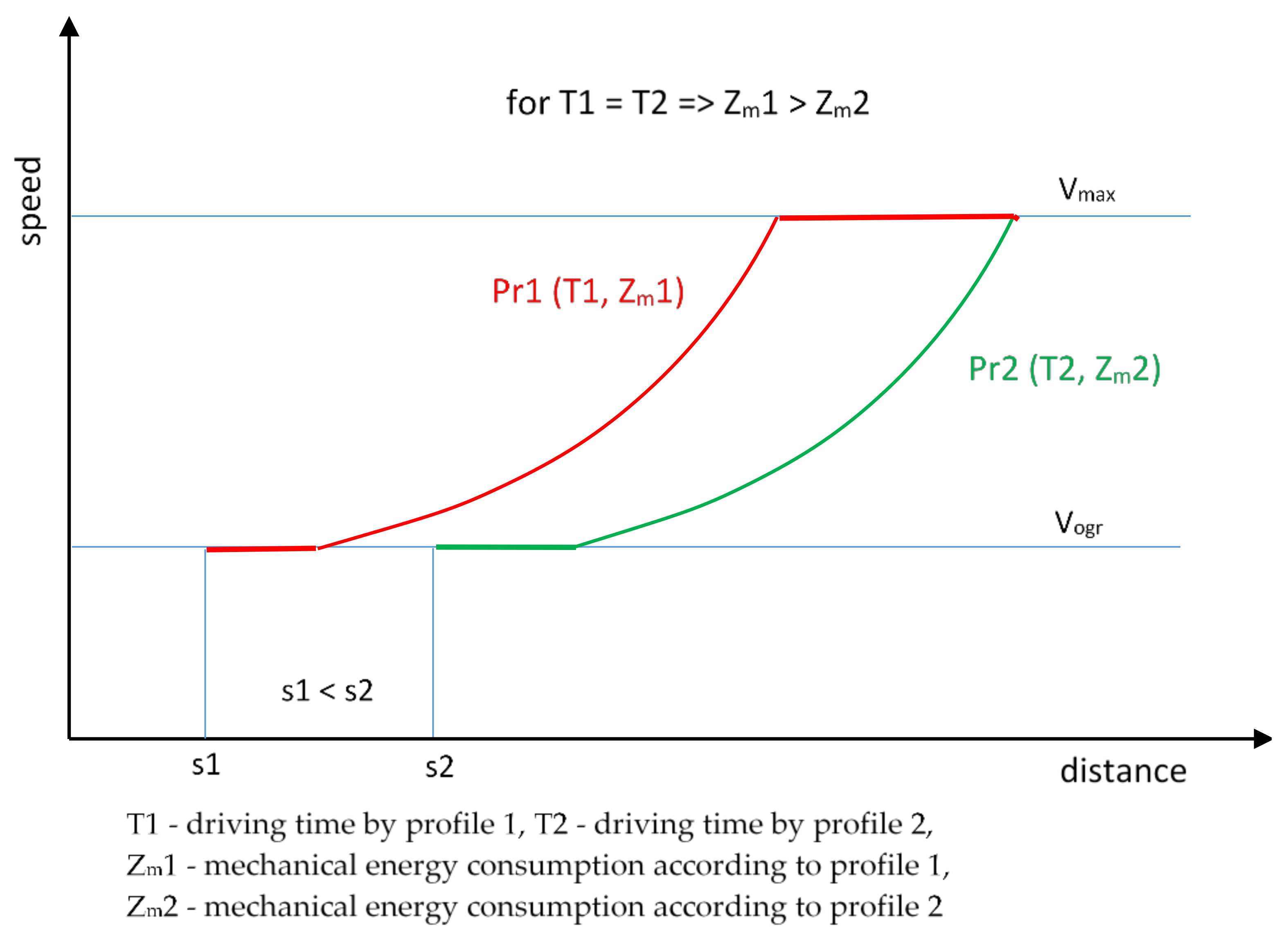
Figure 1 shows the two train speed profiles. The Pr1 profile represents the case of excessive extension of train running time resulting in loss of distance (s1 < s2), where “s” is location, relative to the train that is moving according to the Pr2 speed profile.

Recovery of the lost distance is only possible by increasing the speed in the Pr1 profile. Running according to the Pr2 profile is therefore more advantageous in terms of energy consumption, and this is due to the need to maintain the speed V_ogr (speed on the limit) with less resistance to movement than at the speed V_max (the maximum speed on the distance) in the Pr1 profile, with more resistance to movement.

For example, according to an adopted train and traffic situation model, considered in the speed range from V_ogr = 40 km/h to V_max = 160 km/h, leveling the distance difference of 1 km requires the Pr1 profile mechanical energy consumption to be higher by approximately 1820 kWh than the train running according to the Pr2 speed profile (error tolerance resulting from traction curve interpolation, as per the method provided in [19]: +0.366 and −0.065).

2.2.2. The Consequence of the Train Losing Speed

The reduction in speed translates into the loss of kinetic energy of the train, as well as into the extension in its running time.

In the case as shown in Figure 2, the train running with the Pr1 speed profile against the Pr2 speed profile must increase speed up to V_max over a shorter time to level the speed difference, which translates into increased energy consumption (higher speed difference, longer travel distance at the maximum speed), as well as a negative impact on the smooth running of the train.

For example, according to the adopted train and traffic situation model, considered in terms of speed, V₁ = 30 km/h, V_ogr = 40 km/h, and V_max = 160 km/h; decreasing the speed difference of 10 km/h requires approximately 1980 kWh more mechanical energy for the Pr1 speed profile compared to a train running according to the Pr2 speed profile (error tolerance as above).

3. Searching for the Optimal Solution

3.1. Area of Acceptable Solutions

The traffic situation represents the running of two trains on the same section of line, on the same track, which in the case of higher speed of the following train, may lead to its stopping in case the preceding train fails to leave the next block distance.

Such a situation is very unfavorable from the point of view of energy consumption; therefore, as far as the timetable allows, a smooth process of the following train approaching the preceding one should be achieved, which is a preliminary process for the virtual connection of trains.

To increase the smooth running of approaching, additional information about the $P^P$ traffic parameters is needed. $P^N$ equipped with ERTMS/ETCS L2 can obtain such information from RBC, although it is not standard information according to the current specification. This information can be used to determine the occupancy time of the next block distance and optimize the run profile.

The extension of the information about the speed of the preceding train allows a more precise speed limit and, therefore, a better selection (from the point of view, among others, of the energy consumption) of the traffic parameters for the following train.

In the considered traffic case, a phenomenon appears that the more we extend the travel time of the following train, the lower the probability we have of speed reduction of that train.

On the other hand, extending of train travel time may impact the timetable, which translates into a delay of train arrival to the appointed stations; it may also cause disturbance in the traffic of other planned train routes. In addition, obtaining the smallest possible distance between trains also increases the capacity of the railway line, which is important on lines with heavy train traffic.

Taking the foregoing into account, the travel time of the train is the key issue, and achieving a smooth run of the train and saving energy consumption must not be at the expense of delaying the train from its scheduled time.

Thus, the task of the authors is to indicate a solution allowing the smooth running of the train to be obtained while maintaining the condition of the train running time in compliance with the timetable on a specified section of the railway line. These solutions are in the form of algorithms for shaping run profiles for different variants of the train approach operational scenario.

The optimization task is to find a solution such that the following train loses the least amount of kinetic energy while maintaining a safe distance from the preceding train.

Figure 3 shows the two speed profiles of the following train, Pr1 and Pr2, limiting the set of solutions sought, shown in blue.

In the case of the Pr1 speed profile, train $P^N$ moves with V_max speed until the distance to the V_ogr speed limit location (point L marked on the figure) requires the application of the so-called service braking; in the paper, the value u_h = 0.5 m/s² (additional braking delay resulting from the application of the train braking force) has been adopted.

A train running according to the speed profile Pr1 achieves the shortest possible travel time to the point L, but it is characterized by the highest mechanical energy consumption, which results from the length of the section on which the V_max speed is maintained, resulting in the highest resistance to movement.

In the case of the Pr2 speed profile, train $P^N$ applies service braking by reducing speed from V_max to V_ogr and then runs at a constant speed V_ogr up to the point L.

A train running with the Pr2 speed profile achieves the longest travel time to point L, but it requires less mechanical energy due to the length of the section where the V_ogr speed is maintained.

In the traffic situation, when train $P^N$ in point L obtains an MA for a further run, the train continues with the V_ogr speed (line Pr3). In the case of the lack of MA for a further run, it commences to brake, with its speed decreasing below V_ogr (line Pr4), and in extreme cases, it stops completely. Lines Pr3 and Pr4 are continuations of the speed profiles from the set of sought solutions.

3.2. Objective Function and Evaluation Criteria

The objective function is to obtain such a speed profile of the following train that it is located the smallest possible distance from the beginning of the next block distance in a time equal to the value of the time needed for the preceding train to leave the block distance, at a speed approximate to the speed of the preceding train.

These values have to take into account the delay time for processing and transmitting the information and maintaining a safe braking distance in each case.

The objective function can be obtained by shaping the speed profile of the following train (Figure 4) in such a way that the speed at its end is equal to the speed of the preceding train leaving the block distance (the OB section in the figure) and that the safe time interval T_OB (from the t_o moment to the t_b moment) and distance (from point O to point B) is kept between trains.

The following factors will be the evaluation criteria for the preceding train: the amount of mechanical energy used, the location, and the speed of the train at the moment of the lapse of time T_OB.

In order to compare the distance travelled and the speed attained in relation to the mechanical energy consumption, the standardization method (calculation of the mechanical energy needed to compensate for the differences) will be used, which is discussed in more detail in Section 7.2.

An additional evaluation criterion will also be the magnitude of the achieved smooth running of the train (as defined in Section 4), taking into account that higher train movement fluency results in less wear and tear on rolling stock running parts and wear and tear on the track surface.

The scope of assessment of the following train will be performed between points A and O, whose distance D, representing the distance between trains P^P and P^N at the beginning of the analysis, can take values in the range:

$$V_{ogr} \left(\frac{o{b}_i}{V_{ogr}}-T_H\right)+S_H \le D \le V_{max} \left(\frac{o{b}_i}{V_{ogr}}-T_H\right)+S_H$$

(4)

where T_H (train braking time when using the braking force F_H) is the minimum time on the S_H (the braking distance of the train when the braking force F_H is applied) route necessary to stop the train from the maximum speed to zero, and T^P_OB = ob_i/V_ogr is the time in which the P^P train will cover the OB section at the assumed V_ogr speed on the i-th block distance, while S1 = V_max (T^P_OB − T_H) + S_H is the distance that the train will travel in the T^P_OB time while moving according to the Pr1 profile (Figure 3), and S2 = V_ogr (T^P_OB − T_H) + S_H is the distance that the train will travel according to the Pr2 profile (Figure 3).

3.3. Assumptions Used to Assess the Solutions

The assumptions made are intended to create objective conditions for comparing different train running variants (different speed profiles) for the traffic movement before a variable speed limit. This comparison shall be based on train run kinematics, resistance forces due to train speed, and the traffic control system, including the ability to give information to the following train about the position and speed of the preceding train.

The conditions for the assumptions and simplifications allowing for the analysis and comparison for various train running scenarios are the method of determining the traction energy consumption (type of energy, calculation method, etc.), the parameters and type of the train, the function describing the resultant of traction force and resistance forces, the inclination, and the track geometry (curvature) on a given section of the railway line.

The traction force variability results from the technical parameters of both the traction vehicle drive and external conditions, i.e., weather conditions (wheel–rail adhesion, wind force), track profile and geometry (curves), usable power in the traction network (in a given place) from the distance of the train from the traction substation, and the number of trains and their sequence time in the supply area of the train in question.

The experience of the driver is also important, as is their method of controlling the drive in terms of adjusting the train speed to technical and operational conditions.

All the above-mentioned conditions and limitations affect the non-linearity of the traction characteristics of a traction vehicle: traction force as a function of train speed.

The method of calculating energy consumption, mechanical energy, adopted for the analysis, relates directly to the speed and traction force of the vehicle, as well as the resistance to train motion depending on the train speed. The adopted assumption makes it possible to ignore the efficiency and type of energy used in the drive (electric or thermal), i.e., the efficiency of energy conversion in a traction vehicle, energy consumption for non-traction needs in the train, etc.

Since the consumption of mechanical energy is the product of the traction force (depending on the speed at a given moment) and the speed, and the change in speed depends on the traction force and resistance to motion, the determination of energy consumption is a complex process. Its determination is possible through the use of approximations and averages in short time intervals. For a specified train running time (acceleration):

$$\mathsf{\Delta }T=m_f\mathsf{\Delta }V/{\displaystyle \sum }_{V1}^{V2}F$$

(5)

where V1 < V2 and ΔV = V2 − V1; we use time intervals that allow, approximately to the actual values, the average value of traction force and resistance to motion to be obtained, as well as the average speed of movement. The more time intervals, the shorter the time interval and the shorter the distance and the smaller the deviation of the mean value from the actual values.

The consumption of mechanical energy is the expenditure of traction energy to overcome the resistance to motion and to change the kinetic energy of the train in the case of increasing the running speed:

$$Z={\displaystyle \sum }_{i=1}^n(F_i V_i\Delta T_i)+\underset{V1}{\overset{V2}{{\displaystyle \int }}}{m}_{f}VdV$$

(6)

where Z is the mechanical energy consumption, F_i is the mean value of the traction force in the time interval ∆T_i, V_i is the average speed in the time interval ∆T_i, n is the number of time intervals, and mf is the mass, taking into account the energy of rotating masses (wheels, gears, etc.).

In order to obtain better readability and unambiguity of the variant differences, the following aspects were omitted from the model, i.e., the influence on traction power of the power supply system (voltage and power), efficiency of the power supply and energy processing system, energy losses resulting from resistance in the running parts of the rolling stock, gradient of the line (the profile of the line section with no gradient was established) and track geometry (no curves and turnouts), and the influence of external conditions, such as the influence on the wheel/rail interaction, the so-called slip effect, the way of driving the train by the driver, etc.

For the purpose of results standardization, we used the interpolation of traction characteristics of a particular traction vehicle; detailed information has been presented in publication [19].

3.4. The Logic of the Research Model

Figure 5 shows the interrelationship of technical aspects to find the optimal solution in the set of admissible solutions.

• F_tr: train traction force (depending on the speed),
• F_opr: train force acting on the train as a result of resistance to movement (depending on the speed and the location),
• F_h: braking force acting on the train as a result of applying the braking system,
• u_h: additional braking delay resulting from the application of the train braking force,
• mf: train weight corrected by the rotating mass factor,
• V_ogr: speed on the limit,
• V_max: the maximum speed on the distance,
• a_R: the maximum permissible acceleration of the train,
• a_H: the maximum train braking delay,
• T_h: train braking time,
• S_h: train braking distance,
• T_r: train startup time,
• S_r: train startup distance,
• T^N_AO: time of the P^N train moving between points A and O,
• V^N_AO: speed of the P^N train moving between points A and O, and
• D: distance between P^P and P^N at the t^N_A and t^P_O moment.

4. Traffic Movement Model

4.1. Traffic Operation

Let us now consider the movement of two consecutive trains, running in the same direction on the same track at a given distance D on a section of a railway line with identical conditions of longitudinal gradient (profile) and track geometry fixed over its whole length, as well as with applied railway traffic control devices. The organization of traffic management for such a case is presented in the book [28]; detailed rules of conduct for drivers are defined in an internal instruction of the infrastructure manager [29] and in the instructions for the conduct of drivers running trains equipped with the ETCS system [30].

At the start of the analysis $t=t_A^N=t_O^P=0,$ train P^P is at point O, and train P^N is at point A, and the D distance between them is a fixed input value for the analysis.

Train P^N at the t^N_A moment is running at the V_max maximum speed allowed at the section, while train P^P at the t^P_O moment is running with the V_ogr limited speed.

The moment at which the analysis ends, $t=t_X^N=t_B^P,$ is when the P^P end of the train passes point B, while the P^N train is located at point s between points A and O. The location of the P^N train and the distance between P^P and P^N are quantities that depend on the P^N train driving variant used.

4.2. Division of the Route

For the purposes of the present considerations, the following traffic situation was assumed. On a route divided into fixed ob_n block distances between stations A and B, two P^P and P^N trains are moving, and they are moving in the same direction (from station A to station B on the same track). Each block distance has its pob_n (start ob_n is in the n-th block distance) beginning at the side from which the train is approaching. The end of the section kob_n is on the opposite side of the section with relation to pob_n. The track between two posts is the considered area of the railway network. The locations of the next pob_n are as follows: s(pob₁) = 0 m, s(pob₂) = 2000 m, s(pob₃) = 4000 m, s(pob₄) = 6000 m (point O in front of it), and s(pob₅) = 8000 m.

4.3. Trains

The train going first will be called the P^P preceding train. The train going second will be called the P^N following train. The trains and the area in which they run are equipped with ERTMS\ETCS L2 equipment. Drivers drive trains on the basis of ETCS DMI (Driver Machine Interface) indications. The following P^N train receives an MA as per specification [31] on the basis of the occupation of block distances. The speed and location of the preceding P^P train is the additional information to the MA for P^N.

4.4. Traffic Operation on the Track

Let us assume that the end of P^P is located at ob₃ (3-th block distance). Then, P^N has z_j (the j-th event) whose EOA (End Of Authority) is to pob₃. This situation does not change until P^P leaves ob₃ (event 1: z1). Train P^N does not know when z1 will occur, so it is running with the maximum speed according to the speed profile. If P^N is moving with a speed greater than P^P, then a situation may happen in which it is forced to initiate service braking and, in the most drastic case, to stop.

5. Train Model

5.1. Static Model

The train model in the conducted experiments focuses on its physical, traction, and braking properties. The physical properties include:

• length of the train,
• mass: m, and
• mass corrected with the rotating mass factor: m_f [27].

Considerations will be made for sample rolling stock:

• train length = 300 m,
• m = 194 T, and
• mf = 213 T.

In the context of braking, it is assumed that its most intense form is service braking with a delay value of a_H = 0.5 [m/s²]. The braking distance in this case (maximum speed of 160 km/h) for the static model is S_H = 1970 m.

5.2. Traction Force

Sample dependence for traction force (interpolation) [19]:

for 0–49 km/h:

$$F_{tr}=200,000\left[\mathrm{N}\right]$$

(7)

for 50–160 km/h:

$$F_{tr}=k_1{V}^2+k_{2}V+k_3=12 V^2-3850 V+350,000 \left[N\right]$$

(8)

• k₁: parameter representing the quantities varying depending on the square of the velocity,
• k₂: parameter representing the quantities varying depending on the speed, and
• k₃: parameter representing the quantities varying independent of the speed.

5.3. Resistance Forces

The run of a train involves resistance to motion. Based on [25], where the formula for determining the resistance to motion is defined, the following dependence describing the force of resistance to motion was assumed:

$$F_{opr}=k_4{V}^2+k_{5}V+k_6=0.57V^2+29V+2161\left[\mathrm{N}\right]$$

(9)

• k₄: parameter representing the quantities varying depending on the square of the velocity,
• k₅: parameter representing the quantities varying depending on the speed, and
• k₆: parameter representing the quantities varying independent on the speed.

5.4. Start-Up

The final equation for the force acting on the train during a start-up can be written as:

$$\mathrm{F}={\mathrm{F}}_{tr}–{\mathrm{F}}_{opr}=\left(k_1-k_4\right)V^2+\left(k_2-k_5\right)V+k_3-k_6,$$

(10)

in simple terms:

$$\mathrm{F}=k_{14}{V}^2+k_{25}V+k_{36}.$$

(11)

The train dynamics in the startup phase is described by the formula [19,23]:

$$T_r={\int }_{V=0}^{Vogr}\frac{m_f}{\left(k_{14}{V}^2+k_{25}V+k_{36}\right)}dV,$$

(12)

$$S_r=m_f{\int }_{V=0}^{Vogr}\frac{V}{\left(k_{14}{\mathrm{V}}^2+k_{25}\mathrm{V}+k_{36}\right)}dV.$$

(13)

For the condition:

$$W=k_{25}^2-4k_{14}{k}_{36}>0\mathrm{and}-W<{\left(k_{25}-2k_{14}V\right)}^2<W,$$

(14)

solution [19]:

$$\begin{gathered} T_r=\frac{m_f}{\sqrt{W}}\left[-ln\left(1-\left(k_{25}+2k_{14}{V}_k\right)/\sqrt{W}\right)+ln\left(1-\left(k_{25}+2k_{14}{V}_p\right)/\sqrt{W}\right)+ln\left(1+\left(k_{25}+2k_{14}{V}_k\right)/\sqrt{W}\right)- \\ ln\left(1+\left(k_{25}++2k_{14}{V}_p\right)/\sqrt{W}\right)\right], \end{gathered}$$

(15)

$$S_r=\frac{m_f}{2k_{14}}\left[ln\left(k_{14}{V}_k{}^2+k_{25}{V}_k+k_{36}\right)-ln\left(k_{14}{V}_p{}^2+k_{25}{V}_p+k_{36}\right)\right]-\frac{k_{25}}{2k_{14}}{t}_r.$$

(16)

5.5. Braking

Braking results from two forces: the force resulting from train resistance, as well as the additional braking force due to the train braking system.

In the case where the additional braking force does not depend on the train speed, the equation for the force acting on the train can be written as:

$$F=F_{opr}+F_h=k_4{V}^2+k_{5}V+k_6+u_h{m}_f$$

(17)

where additional braking delay resulting from the application of the train braking force $u_h\in U=\left[-u_H, 0\right], u_H=F_H/m_f$, which is the maximum train braking delay (F_H—maximum permissible braking force) allowed under the applicable technical conditions on a given railway line.

Representing factor u_h m_f as a parameter k₇, independent of the train speed, the equation for the force acting during braking takes the following form:

$$F=F_{opr}+F_h=k_4{V}^2+k_{5}V+k_6+k_7$$

(18)

in simple terms:

$$F=k_4{V}^2+k_{5}V+k_{67}$$

(19)

The train dynamics in the braking phase is described in the book [23], and on the basis of the formulas presented, the analysis of conditions for the derived dependencies in the paper was made [19]:

$$T_h=\underset{Vmax}{\overset{Vogr}{{\displaystyle \int }}}\frac{m_f}{\left(k_4{V}^2+k_{5}V+k_{67}\right)}dV$$

(20)

$$S_h=m_f\underset{Vmax}{\overset{Vogr}{{\displaystyle \int }}}\frac{V}{\left(k_4{\mathrm{V}}^2+k_5\mathrm{V}+k_{67}\right)}dV$$

(21)

Condition: $W=k_5^2-4k_4{k}_{67}<0$ and

$$\mathrm{for}:k_5^2<4k_4{k}_{67}\mathrm{and}{k}_4>0i{k}_{67}>0\mathrm{or}\mathrm{for}:k_5^2<4k_4{k}_{67}\mathrm{and}{k}_4<0and{k}_{67}<0$$

(22)

solution [19]:

$$T_h=\frac{2m_f}{\sqrt{\left(-W\right)}}\left[arctg\left(\frac{2k_4{V}_k+k_5}{\sqrt{\left(-W\right)}}\right)-arctg\left(\frac{2k_4{V}_p+k_5}{\sqrt{\left(-W\right)}}\right)\right]$$

(23)

$$S_h=\frac{m_f}{2k_4}\left[ln\left(k_4{V}_k{}^2+k_5{V}_k+k_{67}\right)-ln\left(k_4{V}_p{}^2+k_5{V}_p+k_{67}\right)\right]-\frac{k_5}{2k_4}{t}_h.$$

(24)

6. Operational Scenario

6.1. General Assumptions

Operational scenarios are a recognized tool for testing the functionality of the ETCS system in different train operations. An example of the application of operational scenarios are the high speed rail in Spain [32] and on Italian Railways [33]; numerous research works are also carried out in laboratory conditions, which were presented in the publication [34].

The operation of the following train is determined by the movement of the preceding train, and therefore, the operational scenarios will be determined by the traffic situation resulting from the three contexts of the preceding train movement (Figure 6):

• Context 1: The P^P train at the start of the simulation is running at the reduced speed of V_ogr = 40 km/h and is moving with such a reduced speed on the whole OB section.
• Context 2: The P^P train at the start of the simulation is running with the reduced speed V_ogr = 40 km/h and then receives information about the release of subsequent block distances, which allows an increase in speed. The change of speed shall be at the maximum allowable acceleration at block distance ob₄.
• Context 3: Train P^P at the start of the simulation is running with the reduced speed V_ogr = 40 km/h and then, due to lack of information on the release of subsequent block distances (ob₅ occupied), starts braking. After stopping, it receives information about the release of subsequent block distances, which makes it possible to increase speed. The change of speed shall be at the maximum allowable acceleration at block distance ob₄.

It takes 10 s for the driver to stop, which results from the driver’s reaction, brake dragging, and switching the P^P systems into the start-up mode.

In the case of the following train, the study assumed four variants of the train speed profile (movement) on the AO section. These variants differ in the following assumptions:

• Variant I: (reference variant) the P^N train is moving based on indications from ERMS/ETCS L2, and based on the information about approaching the EOA (End Of Authority) (at distance of 2000 m), it starts service braking.
• Variant II: (reference variant) train P^N is moving based on ERMS\ETCS L2 indications and additionally receives information about the occupancy of subsequent block distances within distance of 6000 m from the place at which it is currently located. The driver switches off the propulsion, and the train is moving in the so-called startup mode until it approaches the EOA and within 2000 m, commences service braking.
• Variant III: the P^N train is moving based on ERMS\ETCS L2 indications, and in addition, it receives the information on the location and speed of train P^P. This information is updated every 10 s (suggested value for the ETCS variable: T_CYCLOC).

Based on an algorithm for optimizing the train speed profile, the drivers are given data at what speed (using the propulsion system to overcome the resistance to motion) or braking force they should apply to continue to run to the location of the EOA place.

• Variant IV: train P^N is moving based on ERMS\ETCS L2 indications, and in addition, it receives information on the location and speed of train P^P. This information is updated every 10 s (suggested value for the ETCS variable: T_CYCLOC).

Based on an algorithm for optimizing the train speed profile, the driver is given data about whether to continue running in the so-called startup mode or to apply (and at what force) the braking of the train in order to reduce the speed until the EOA place.

The first two variants assume that the traffic management technique is in accordance with current practice and does not use additional information about the movement parameters of the P^P preceding train. Two others assume that such information is sent to P^N together with z_j and will be used in the run-shaping profile algorithm.

All variants of the operational scenario assume a similar initial situation. The preceding train is running at a constant speed of V^P_O = 40 km/h (speed of the P^P train at point O). The following train is running at a speed of V^N_A = 160 km/h (speed of the P^N train at point A). Train P^P is at the location just before deceleration ob₃ (3-th block distance).

6.2. Variant 1 (Red)—Run at Maximum Speed without Consideration of s^P and V^P

Variant 1 assumes the initial conditions as described in Section 4.1. It is also assumed that P^N has no information on V^P and s^P (speed of the P^P train at point s). It only has the MA and is moving with a maximum speed of V_max = 160 km/h.

At the moment of t_z11, event z11 occurs when P^P leaves ob₃, and zjP^N (MA for the following train) extends to pob₄. At the t_z12 moment, the event z12 occurs, consisting of P^N reaching the last safe location where it commences service braking to pob₄. Until the t_z13 moment (ob₄ release event by P^P) and when reaching the safe distance to pob₄, the P^N train continues braking, until it stops.

At the t_z13 moment, event z13 occurs, consisting of extending zjP^N to pob₅, and P^N passes from the braking phase to the acceleration phase.

The course of the operational scenario (t_z1–z3) can be divided into the following stages:

$$T_{z11–z13}=T_{z11–z12}+T_{z12–z13}$$

(25)

where:

• T_z11–z12: train running time at the maximum speed (T_zi-zj: travel time between events i and j),
• T_z12–z13: train running time at the braking phase,

so:

$$T_{z11–z13}=T_{Vmax}+T_h$$

(26)

$$T_{Vmax}=\frac{\left(D-S_h\right)}{V_{max}}$$

(27)

where T_Vmax is the time of running at maximum speed; T_h and S_h shall be determined on the basis of dependencies (18 and 19) described in Section 5.5.

We are analyzing the mechanical energy consumption of P^N for variant 1 between events z11 and z13 (T_z11–z13):

• Z_z11–z12: consumption related to sustaining speed V_max, and
• Z_z12–z13: no mechanical energy consumption,

resulting in

$$Z_m=Z_{z11–z12}=F_{tr max} (D-S_h)$$

(28)

where: F_{tr max} is the traction force to maintain the maximum speed.

6.3. Variant 2 (Orange): Idle Running without Consideration of V^P

Variant 2 assumes the initial conditions as described in Section 4.1.

It is also assumed that P^N has information about S^P (information about the occupancy of the ob₄ section), has the MA, and reduces its speed from the maximum value of V_max = 160 km/h as a result of switching off the propulsion and running at the so-called idle movement (deceleration mode as a result of traffic resistance forces).

At the t_z21 moment, event z21 occurs when P^P leaves ob₃, and zjP^N extends to pob₄. P^N is running at the so-called idle movement mode until t_z22, when the event z22 occurs, consisting of P^N reaching the last safe location, where it commences service braking to pob₄.

Until the t_z23 moment (when P^P slows down on section ob₄), train P^N continues braking, and it does so in the case of reaching the safe distance to pob₄, until it stops.

At the t_z23 moment, event z23 occurs, consisting of extending zjP^N to pob₅, and P^N passes from the braking phase to the acceleration one.

The course of the operational scenario (t_z1–z3) can be divided into the following stages:

$$T_{z21–z23}= T_{z21–z22}+T_{z22–z23}$$

(29)

where

• T_z21–z22: train running time at the so-called idle movement mode and
• T_z22–z23: train running time at the braking phase,

so:

$$T_{z21–z23}=T_w+T_h$$

(30)

where T_w, S_w is the time and distance of operation at the so-called inert movement (speed decreases due to resistance forces); T_h, S_h are determined on the basis of dependencies (18 and 19) described in Section 5.5, taking into account that for T_w, S_w force F_h is equal to zero, and the force acting on the train is calculated according to the dependence:

$$F=F_{opr}=k_4{V}^2+ k_{5}V+k_6$$

(31)

We are analyzing the mechanical energy consumption P^N for variant 2 between events z21 and z23 (t_z21–z23):

Z_z21–z22 and Z_z22–z23 indicate no mechanical energy consumption,

resulting in:

$$Z_m=Z_{z21–z22}+Z_{z22–z23}=0.$$

(32)

6.4. Variant 3 (Blue): Run at Variable Speed, with Consideration of s^P and V^P

Variant 3 assumes the initial conditions as described in Section 4.1.

It is also assumed that P^N has information about s^P and V^P, has the MA, and reduces its speed from maximum value of V_max = 160 km/h to V_ogr = 40 km/h by controlled braking of the train and running over part of the route at a set speed of V_x.

At the t_z31 moment, event z31 occurs when P^P leaves ob₃, zjP^N extends to pob₄, and P^N receives information about the P^P train, i.e., location s^P and speed V^P_O (information update every 10 s), and the length of distance ob₅.

On the basis of the provided information, distance D between trains is calculated, and the estimated train running time P^P to point B (the predicted moment of leaving distance ob₅) is calculated according to the dependence:

$$T_{OB}^P=\frac{V_O^P}{S_{ob5}}$$

(33)

For the variant with speed control, it is assumed that P^N should arrive at distance D* = D − S_H, where S_H is the braking distance of train P^N.

The following dependencies will be used to obtain the expected time at a given distance:

$$T_{OB}^P=T_h^N+T_x^N$$

(34)

$$D^{*}=S_h^N+S_x^N$$

(35)

where T^N_h, S^N_h are the braking time and distance, determined according to Formulas (18) and (19), depending, among others, on the value of braking delay a_h; T^N_x = V_x/S_x is the travel time P^N at a constant speed; and S^N_x is the distance travelled by P^N at constant speed V_x.

Taking into consideration:

$$V_x=\frac{S_x}{T_x}=\frac{(D^{*}-S_h)}{(T_{OB}^P-T_h)}$$

(36)

We are looking for such braking force, F_h = m_f u_h, that the force acting on a train, consisting of the sum of the movement resistance force and the braking system force,

$$F=F_{opr}+F_h=F_{opr}+m_f u_h=m_f a_h$$

(37)

will allow us to determine the braking time and distance for which the optimum speed

$$V_x^N: V_{ogr} < V_x < V_{max}$$

(38)

will meet the minimum energy consumption criterion:

$$Z_m=F_{tr}{S}_x=m_f\left(k_4{V}_x{}^2+k_5{V}_x+k_6\right) S_x\to minimum$$

(39)

At the t₃₁ moment, train P^N commences braking, with a delay a_h, from maximum speed V_max to speed V_x. At moment t₃₂, event z32 occurs when the P^N train acquires speed V_x and continues to move on for the designated distance S_x, using the propulsion system to balance the resistance forces and maintain the preset speed V_x.

At moment t₃₃, event z33 occurs, where P^N has covered the designated distance S_x and is braking, with delay a_h, from set speed V_x to speed V_ogr limit.

At moment t₃₄, event z₃₄ occurs, consisting of P^N reaching the point at which it is correcting the braking force to the last safe location at which it can receive an update of zj to pob₄.

When approaching the pob4 within a safe distance, it is stopped.

The course of the operational scenario (T_z31–z34) can be divided into three stages:

$$T_{z31-z34}=T_{z31-z32}+T_{z32-z33}+T_{z33-z34}$$

(40)

where

• T_z31–z32: train running time at the braking phase,
• T_z32–z33: train running time at sustained speed V_x, and
• T_z33–z34: train running time at the braking phase,

so:

$$T_{z31-z34}=T_h/2+T_x+T_h/2$$

(41)

where T_h and S_h are determined on the basis of the dependence described in Section 5.5. (18 and 19), while T_x is determined by Equation (34):

$$T_x=\frac{(D^{*}-S_h)}{V_x}$$

(42)

We are analyzing the mechanical energy consumption of P^N for variant 3 between events z31 and z33 (T_z31–z33):

Z_z31–z32 and Z_z33–z34 indicate no mechanical energy consumption, and

Z_z32–z33 indicates the energy consumption for balancing the resistance to movement and maintaining speed V^N_x,

and finally:

$$Z_{\mathrm{m}}=Z_{\mathrm{z}32-\mathrm{z}33}=F_{tr}{\mathrm{S}}_x$$

(43)

6.5. Variant 4 (Green): Run with Braking Control Including s^P and V^P

Variant 4 assumes the initial conditions, as described in Section 4.1.

It is also assumed that P^N has information about s^P and V^P, it has the MA, and it reduces its speed from the maximum value of V_max = 160 km/h to V_ogr = 40 km/h as a result of switching off the propulsion and controlled braking of the train.

At moment t_z41, event z41 occurs when P^P leaves ob₃, zjP^N extends to pob₄, and P^N receives information about train P^P, i.e., about location s^P and speed V^P_O (information is updated every 10 s).

Based on the provided information, the distance D between trains is calculated, and the speed of train P^P is compared to the speed of P^N.

The braking delay is determined from the following dependence described in Section 2.1. (Formula (3)):

$$a_h=({(V_s^P)}^2-\left(V_s^N{)}^2\right) / \left(2 D^{*}\right)$$

(44)

where D* = D − S_H, S_H is the braking distance calculated for train P^N from speed V_ogr to V = 0.

In the case when V^N_t ≤ V^P_t (speed of the P^N and P^P train at “t” moment), train P^N uses propulsion to increase speed, with its acceleration determined by dependence:

$$a_r=({(V_t^N)}^2-\left(V_t^P{)}^2\right) / \left(2 D^{*}\right)$$

(45)

The P^N train is moving according to the aforementioned dependencies until the tz42 moment, when the z42 event occurs, consisting of P^N reaching the last safe location at which service braking is invoked to the last safe location at which the train must obtain an extension for the MA without the need to brake before the EOA.

Until the t_z43 moment (when P^P is leaving ob₄), train P^N continues braking.

At moment t_z43, event z43 occurs, consisting of extending zjP^N to pob₅, and P^N passes from the braking phase to the acceleration phase.

The course of the operational scenario (t_z41–z43) can be divided into the following stages:

$$T_{z41-z43}=T_{z41-z42}+T_{z42-z43}$$

(46)

where:

• T_z41–z42 is the train running time with controlled delay or acceleration, and
• T_z42–z23 is the train running time at the braking phase,

so:

$$T_{z21-z23}=T_h\mathrm{or}{T}_{z21-z23}=T_h+T_r$$

(47)

where T_h, T_r, S_h, and S_r are determined on the basis of dependencies (13, 14, 18, 19) described in Section 6.5. and calculated on the basis of delay or acceleration, following (42) and (43).

We are analyzing the mechanical energy consumption of P^N for variant 4 between events z41 and z43 (T_z41–z43):

Z_z41–z42 represents the mechanical energy consumption in the case of V^N_t ≤ V^P_t, when increasing the speed of a train with acceleration a_r,

Z_z41–z42 represents no mechanical energy consumption in the case of V^N_t > V^P_t, when reducing the speed with delay a_h, and

Z_z42–z43 represents no mechanical energy consumption.

The mechanical energy consumption is the sum of the energy consumed to overcome the resistance to movement (determined for the average speed of F_Vśr = m_f a_r and the distance within the range of ΔS_i) and the change of kinetic energy of the train from speed V₁ to speed V₂, according to the dependence:

$$Z_{tr}={\displaystyle \sum }_{i=0}^{n_1} m_f a_r \Delta S_i+\underset{V1}{\overset{V2}{{\displaystyle \int }}} m_{f}V dV$$

(48)

where n₁ = T₁/∆t is number of time intervals for which Vśr_i and ΔS_i have been determined at the i section.

7. Studies

7.1. Assumptions for the Studies

The study was carried out from moment t = t^P_O = 0 until t = t^P_B, when the preceding train leaves block distance OB and the following train obtains the MA for section OB.

At moment t = t^P_B, different variants of the following train movement were obtained, the differences of which were mainly due to the length of the distance covered (measured from point A) and the changes of speed on a given run route.

The braking routes, according to Ie-4 [35] are presented in

Table 1. The required speed on the braking distance on the lines of PKP Polskie Linie Kolejowe S.A.

Distance to the stopping point [m]:
1300	1000	700	400	100
Maximum permissible speed [km/h]:
160	140	100	60	0

Ls = 2000: distance to the location of the EOA for further movement, taking into account train braking distance, distance between semaphores, and their visibility. This distance allows a train to be stopped from 160 km/h to the location of the MA by implementing the service braking. Cyclic calculation occurs every 1 s. Error tolerance resulting from the interpolation of traction characteristics: +0.366 and −0.065, according to the method provided in [19]).

.

7.2. Standardization of Results

A comparison of the variants in terms of mechanical energy consumption alone is not conclusive. It should be noted that a train which has had a shorter route or is moving at a lower speed will have to use additional energy to compensate for those values in order to maintain the scheduled time of the train at the next section of the route.

Therefore, for the purpose of comparing the variants, we applied the so-called standardization of the volumes, in this case consisting in calculating the amount of mechanical energy consumption for the purpose of compensating for the differences obtained.

As shown in Figure 7, for each variant, we calculated the required mechanical energy consumption for reaching point B by train P^N, using the maximum allowable acceleration. In the case of differences in speed, we additionally calculated the mechanical energy needed to increase the speed to the highest value obtained in one of the variants (in Figure 7, variant 4: green).

The mechanical energy consumption for each variant amounts to

$$Z_{sB}^N=F_{sB}^N S_{sB}^N+m_f \frac{\left(V_{N max}^2-V_N^2\right)}{2}$$

(49)

where F^N_sB is a traction force required to balance the resistance to movement over section S^N_sB from point s to point B for the N-th variant; V_Nmax is the highest speed obtained in the N variant at point B.

The final comparison of variants was to compare the sum of the mechanical energy consumption of the P^N trains on route S_AB^N plus the mechanical energy needed to compensate for speed differences.

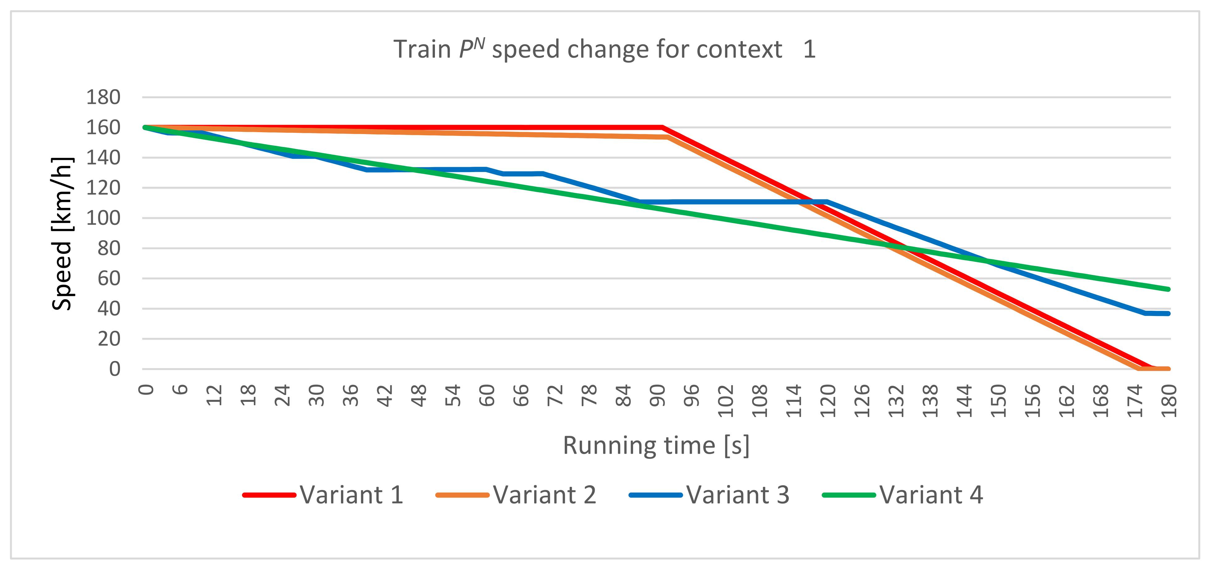
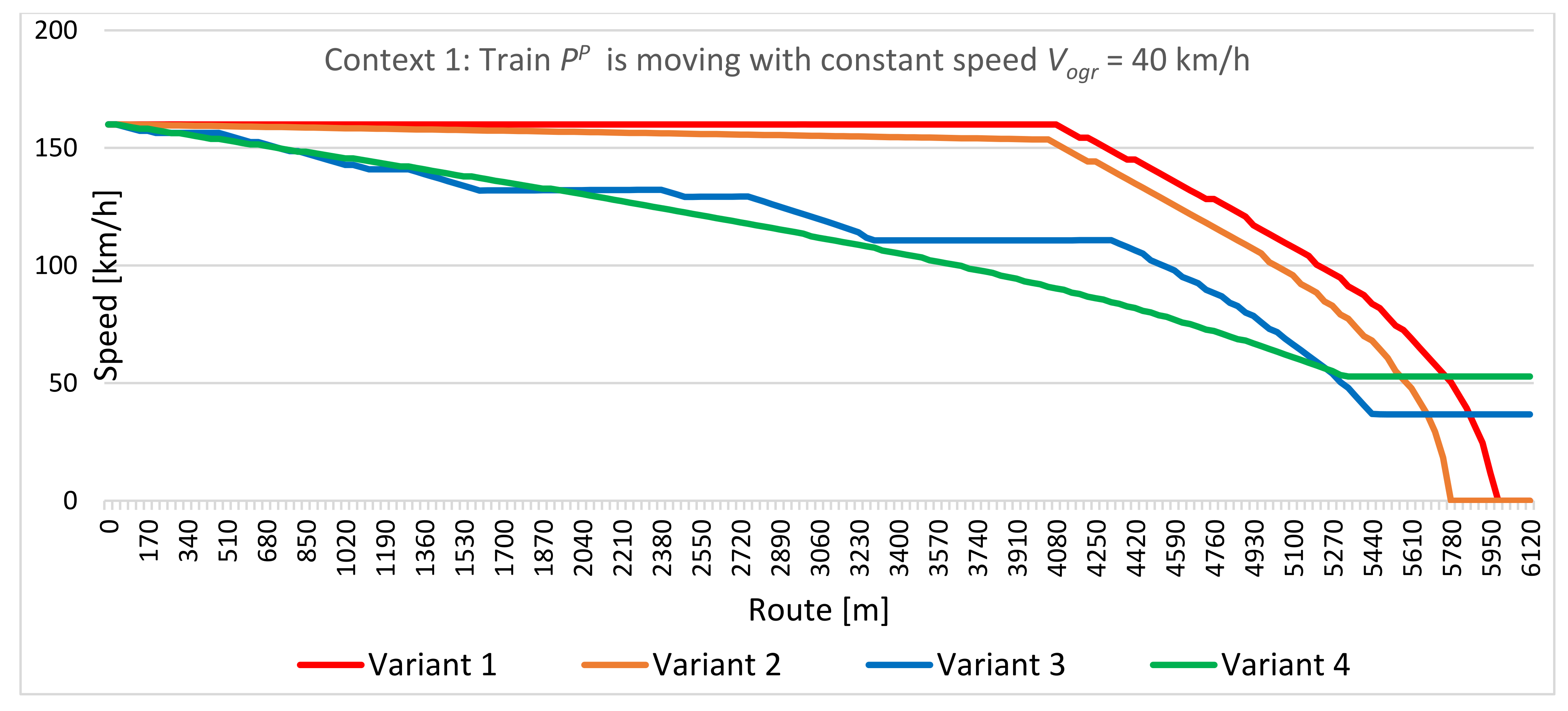
7.3. Simulation Results for Context 1

In variants 1 and 2, it was necessary to stop the train, even though the preceding train was moving at a constant speed without stopping.

Variant 4 was the most profitable one in terms of energy consumption, which also allowed the train to operate most smoothly.

The results for all variants for context 1 are shown in the

Table 2. Results for the variants P^N according to Context 1 P^P.

Context 1: The Preceding Train Is Moving with Constant Speedm Vogr = 40 km/h; It Is Leaving Block Distance ob4 after Time TOB = 180 s
The Following Train	Moment of Measurement	The Route Travelled	Speed	Consumed Mech. Power
	[s]	[m]	[km/h]	[kWh]
Variant 1:	180	5958	0	4.753
Variant 2:	180	5771	0	0.000
Variant 3:	180	5478	37	2.787
Variant 4:	180	5317	53	0.000

while the standarization of results is presented in the

Table 3. Standardization of results for context 1.

Standardization of Results at Point “B” (Increasing Speed with Maximum Acceleration). Context 1: Train PP Is Moving with Constant Speed Vogr = 40 km/h; It Is Leaving Block Distance ob4 after Time TOB = 180 s
The Following Train	Mechanical Energy Consumption in Simulation	Mech. Energy Consumption to Approach Point “B”	Speed at Point “B”	Mechanical Energy Consumption to Attain the Highest Speed	Total Mechanical Energy Consumption
	[kWh]	[kWh]	[km/h]	[kWh]	[kWh]
Variant 1:	4.753	46.979	140	7.914	59.646
Variant 2:	0.000	50.949	144	5.426	56.376
Variant 3:	2.787	50.294	148	1.479	54.560
Variant 4:	0.000	49.861	151	0.000	49.861

.

A graphical representation of the results for all variants for context 1 is shown in Figure 8 and Figure 9.

7.4. Simulation Results for Context 2

Variants 1 and 2 were the most favorable ones from the point of view of energy consumption and smooth running of the train. This is because there was no need to reduce the speed of the trains, as the preceding train leaves ob4 before the trains approach the last location where they need to start braking before the EOA.

Information transmitted every 10 s in variants 3 and 4 had, in this case, an adverse effect on the course of the following trains: they adjusted their speed to the preceding train, which, taking into consideration the 10 s delay, caused unnecessary reduction of the speed of the following train.

The effect of the volume of the distance between trains at time t = 0 is worth noting. When the distance was shortened from D = 6000 m to D = 4600 m, the speed profiles for the individual variants of Context 2 changed, and they resembled the variant profiles for Context 1. This means that variants 1 and 2 were no longer the most favorable with respect to variants 3 and 4, due to the fact that train P^N in variants 1 and 2 approached the last point too quickly, at which it needed to brake before the EOA.

The above case shows that it is necessary to consider how to interpret and create a speed profile for the P^N train to consider the trend of the change of the speed of the preceding train and the expected distance between trains.

The results for all variants for context 2 are shown in the

Table 4. Results for variants PN according to context 2.

Context 2: Train PP Is Accelerating with Maximum Acceleration; It Is Leaving Block Distance ob4 after TOB = 70 s
The Following Train	Moment of Measurement	The Route Travelled	Speed	Consumed Mech. Power
	[s]	[m]	[km/h]	[kWh]
Variant 1:	70	3111	160	3.656
Variant 2:	70	3063	155	0.000
Variant 3:	70	3102	160	6.047
Variant 4:	70	2820	138	0.405

while the standarization of results is presented in the

Table 5. Standardization of results for context 2.

Standardization of Results at Point “B” (Increasing Speed with Maximum Acceleration). Context 2: Train PP Is Accelerating with the Maximum Acceleration; It Is Leaving Block Distance ob4 after TOB = 70 s
The Following Train	Mechanical Energy Consumption in Simulation	Mech. Energy Consumption to Approach Point “B”	Speed at Point “B”	Mechanical Energy Consumption to Attain the Highest Speed	Total Mechanical Energy Consumption
	[kWh]	[kWh]	[km/h]	[kWh]	[kWh]
Variant 1:	3.656	5.798	160	0.000	9.455
Variant 2:	0.000	9.446	160	0.000	9.446
Variant 3:	6.047	5.798	160	0.000	11.845
Variant 4:	0.405	21.361	160	0.000	21.766

.

A graphical representation of the results for all variants for context 2 is shown in Figure 10 and Figure 11.

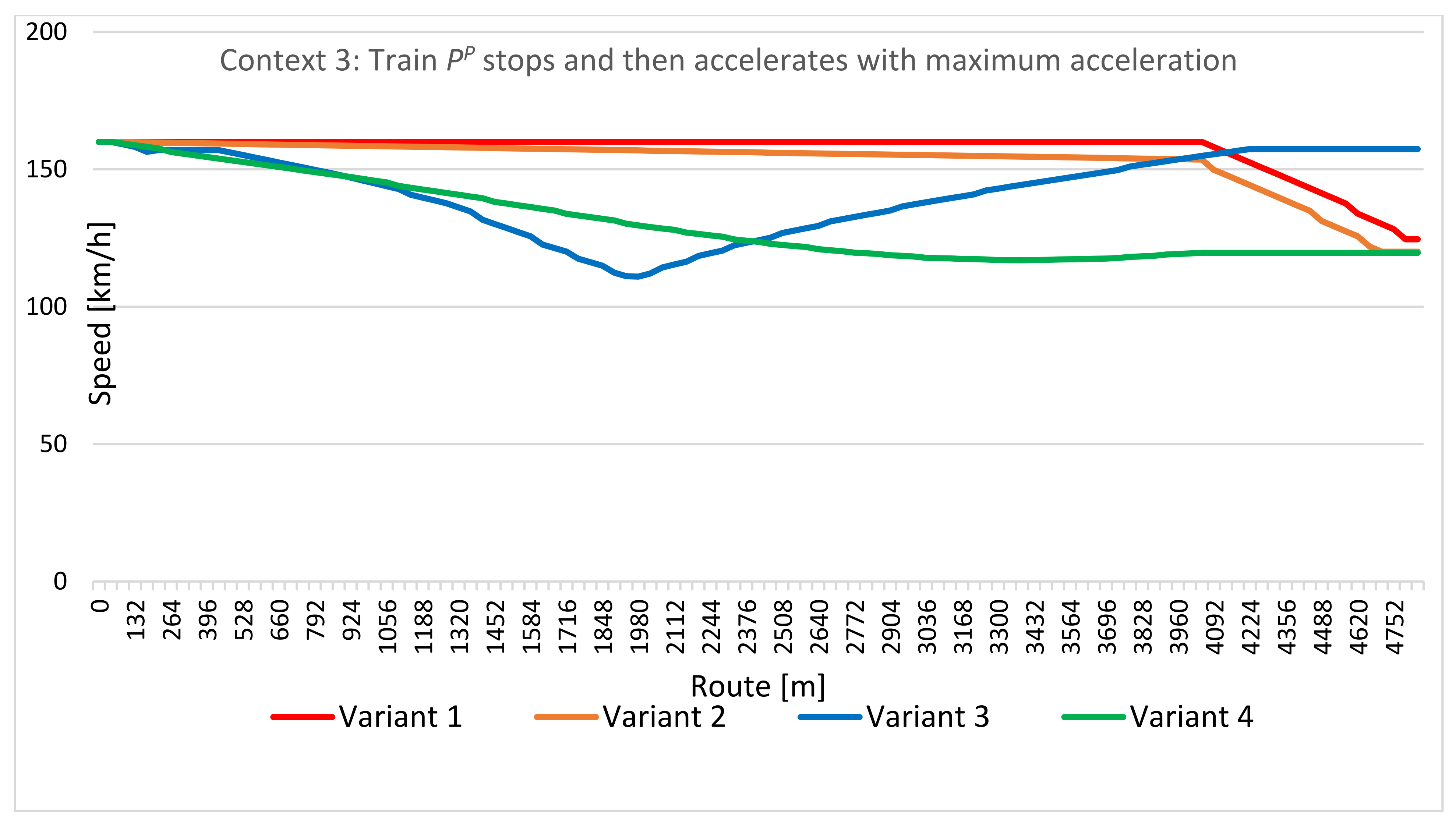
7.5. Simulation Results for Context 3

From the energy consumption point of view, variant 2 was the most beneficial, while from the point of view of smooth running of the train, variant 4 was the most beneficial.

It is worth noting that the profile according to variant 3 is close to the speed profile of the preceding train (there was a time and distance interval as a result of attaining the similar speed of both trains), which can be important when applying the so-called mobile block distance.

The results for all variants for context 3 are shown in the

Table 6. Results for the variants of train P^N according to context 3.

Context 3: Train PP Stops and Then Accelerates with Maximum Acceleration; It Leaves the Block Distance ob4 after Time TOB = 110 s
The Following Train	Moment of Measurement	The Route Travelled	Speed	Consumed Mech. Power
	[s]	[m]	[km/h]	[kWh]
Variant 1:	110	4795	125	4.753
Variant 2:	110	4691	120	0.000
Variant 3:	110	4211	157	32.179
Variant 4:	110	4009	120	2.116

while the standarization of results is presented in the

Table 7. Standardization of results for Context 3.

Standardization of Results at Point “B” (Increasing Speed with Maximum Acceleration). Context 3: Train PP Stops and Then Accelerates with Maximum Acceleration; It Is Leaving the Block Distance ob4 after Time TOB = 110 s
The Following Train	Mechanical Energy Consumption in Simulation	Mech. Energy Consumption to Approach Point “B”	Speed at Point “B”	Mechanical Energy Consumption to Attain the Highest Speed	Total Mechanical Energy Consumption
	[kWh]	[kWh]	[km/h]	[kWh]	[kWh]
Variant 1:	4.753	26.757	160	0.000	31.510
Variant 2:	0.000	29.434	160	0.000	29.434
Variant 3:	32.179	6.731	160	0.000	38.910
Variant 4:	2.116	30.751	160	0.000	32.867

.

A graphical representation of the results for all variants for context 2 is shown in Figure 12 and Figure 13.

8. Discussion and Conclusions

This paper presented the results of a study on the energy efficiency and smooth running of a train on the route while approaching another train. Such a situation occurs when trains follow each other on the same track in the same direction, which is a starting point for creating train traffic management with prospective use of the so-called virtual distance between trains. This paper presented the models necessary for carrying out the study and characterizes the experimental field that was used for the study. We analyzed four variants of the train driving technique, proposing two solutions, taking advantage of the fact that the following train receives the values of operation parameters of the preceding train.

We carried out studies with respect to all variants for three different contexts of the movement of the preceding train.

On the basis of the indicated literature (chapter 1), it was expected that benefits would be obtained in shortening the distance between trains as a result of connecting trains in the so-called convoys (virtual distance), as well as thanks to the development of the ERTMS/ETCS system.

The authors of the work focused on a selected characteristic case of a traffic situation: trains approaching each other at a distance of the influence of the position of the preceding train on the following train, and as a result of the analysis of various variants and contexts of the situation, they assessed the possibility of obtaining the above-mentioned benefits.

The tests allowed this study to obtain positive results for checking the influence of information from the preceding train (train speed) on energy saving and running smoothness of the following train, as a result of adjusting the speed of the following train to the speed of the preceding train.

The obtained case of the most profitable train driving, according to variant 4 for context 1, confirms the possibility of obtaining the optimal solution in the defined area of acceptable solutions.

It should be noted that not every variant and operational context allows for obtaining the expected results, e.g., context 2 showed that variants 1 and 2 (without adjusting the speed of the train following the preceding train) remained the most advantageous.

In order to assess the impact of changes in the parameters of the railway line (increasing the resistance forces) on the results, simulations were made for the line section inclination from −0.7‰ up to +6.0‰.

The simulation showed that for the increase in resistance to motion,

• for context 1, variant 3 and 4 remained the most favorable, reducing the difference between variant 3 and 4;
• for context 2, the results of all variants become equal, and variant 1 and 2 remained the most favorable; and
• for context 3, variant 1 and 2 deteriorated with respect to variant 3 and 4, and variant 4 deteriorated the least.

As it can be seen from the simulation, the benefits are strongly influenced by the context of the preceding train movement and the distance between trains. The frequency of transmission of information about traffic parameters, P^P, i.e., train location and speed, to train P^N is also important.

A large spectrum of possibilities for creating a speed profile on the basis of data of the preceding train (location and speed) provides good reasons for further analyses of this issue.

The applied variety of studies has showed that the exchange of information between trains about the operation parameters can significantly improve the energy efficiency and smooth running of the train. At the same time, there are situations where having the information slightly reduces efficiency, and this occurs when there is significant variability in the operational parameters of the preceding train. These observations will be the input to enhance the proposed techniques in further stages of the research.

References

- European Commission. A Strategy for Sustainable and Intelligent Mobility—European Transport on the Road to the Future; Communication COM2020 of 9.12.2020; European Commission: Brussels, Belgium, 2020. [Google Scholar]
- EUAR. ETCS Test Plan and Methodology for Ss-076 (ERA_ERTMS_040092); European Union Agency for Railways: Valenciennes, France, 2017. [Google Scholar]
- Strossenrauten, H. Energy-efficient driving. In Proceedings of the 2nd UIC Railway Energy Efficiency Conference (UIC-REEC), Paris, France, 4–5 February 2004. [Google Scholar]
- UIC. Evaluation of Energy Efficiency Technologies for Rolling Stock and Train Operation of Railways. December 2016. Available online: http://www.railway-energy.org (accessed on 10 September 2021).
- IEEE Std. 1474.1-2004—IEEE Standard for Communication Based Train Control Performance Requirements and Functional Requirements; Institute of Electrical and Electronics Engineers: New York, NY, USA, 2004. [Google Scholar]
- Kochan, A.; Koper, E.; Wontorski, P. Automatic train driving—Analysis of requirements. In Proceedings of the 10th International Scientific and Technical Conference Logistic Systems Theory and Practice, Transport Certification Centre at the Faculty of Transport, Warsaw University of Technology, Warsaw, Poland, April 2018; pp. 1–14. Available online: https://pnpw-transport.publisherspanel.com/resources/html/article/details?id=208720&language=en (accessed on 12 November 2021).
- Keskin, K.; Karamancioglu, A. Energy-Efficient Train Operation Using Nature-Inspired Algorithms. J. Adv. Transp. 2017. [Google Scholar] [CrossRef] [Green Version]
- Kochan, A.; Koper, E. Mathematical Model of the Movement Authority in the ERTMS/ETCS System. In Research Methods and Solutions to Current Transport Problems; Siergiejczyk, M., Krzykowska, K., Eds.; Springer: Cham, Switzerland, January 2020; pp. 215–224. Available online: https://www.researchgate.net (accessed on 10 September 2021).
- Emery, D. Enhanced ETCS L2/L3 train control system. WIT Trans. State-Art Sci. Eng. 2010, 46, 112–122. [Google Scholar]
- Koper, E.; Kochan, A.; Gruba, Ł. Simulation of the Effect of Selected National Values on the Braking Curves of an ETCS Vehicle. In Development of Transport by Telematics; Mikulski, J., Ed.; Springer: Cham, Switzerland, 3 August 2019; pp. 17–31. [Google Scholar]
- Koper, E.; Kochan, A. Testing the Smooth Driving of a Train Using a Neural Network. Sustainability 2020, 12, 4622. [Google Scholar] [CrossRef]
- Quaglietta, E.; Wang, M.; Goverde, R.M.P. A multi-state train-following model for the analysis of virtual coupling railway operations. J. Rail Transp. Plan. Manag. 2020, 15, 100195. [Google Scholar] [CrossRef]
- ERA; UNISIG; EEIG, ERTMS Users Group. System Requirements Specification; REF: SUBSET-026-1, ISSUE: 3.6.0, DATE: 13/05/2016 r; European Union Agency for Railways: Valenciennes, France, 13 May 2016. [Google Scholar]
- Flammini, F.; Marrone, S.; Nardone, R.; Petrillo, A.; Santini, S.; Vittorini, V. Towards Railway Virtual Coupling. In Proceedings of the 2018 IEEE International Conference on Electrical Systems for Aircraft, Railway, Ship Propulsion and Road Vehicles & International Transportation Electrification Conference (ESARS-ITEC), Nottingham, UK, 7–9 November 2018. [Google Scholar] [CrossRef]
- Mitchell, I.; Goddard, E.; Montes, F.; Stanley, P.; Muttram, R.; Coenraad, W.; Poré, J.; Andrews, S.; Lochman, L. Ertms Level 4, Train Convoys or Virtual Coupling; IRSE International Technical Committee: Tokyo, Japan, 2016. [Google Scholar]
- Kwaśnikowski, J.; Gramza, G. Analiza wybranych zakłóceń w ruchu kolejowym. Politechnika Poznańska. Probl. Eksploat. 2007, 89–96. Available online: https://scholar.google.com.sg/scholar?hl=zh-CN&as_sdt=0%2C5&as_vis=1&q=ANALIZA+WYBRANYCH+ZAK%C5%81%C3%93CE%C5%83+W+RUCHU+KOLEJOWYM+&btnG= (accessed on 12 November 2021).
- Kwaśnikowski, J.; Gramza, G. Wpływ zakłóceń ruchu i profilu trasy na zużycie energii przez lokomotywę elektryczną EU07 prowadzącą pociąg pasażerski. Pr. Nauk. Politech. Radom.–Elektr. 2005, 1, 131–136. [Google Scholar]
- Luetki, M. Evaluation of energy saving strategies in heavily used networks by implementing an integrated real-time rescheduling system. WIT Trans. Built Environ. 2008, 103, 349–358. [Google Scholar]
- Szkopiński, J. Selected problems of train motion optimization. Prace naukowe. Politechnika Warszawska. Transport. WUT J. Transp. Eng. 2020, 131, 59–77, ISSN: 1230-9265. Available online: https://pnpw-transport.publisherspanel.com/resources/html/article/details?id=214837 (accessed on 10 September 2021). [CrossRef]
- Liu, W.; Tang, T.; Su, S.; Yin, J.; Cao, Y.; Wang, C. Energy-Efficient Train Driving Strategy with Considering the Steep Downhill Segment. Processes 2019, 7, 77. Available online: https://0-www-mdpi-com.brum.beds.ac.uk/2227-9717/7/2/77 (accessed on 10 September 2021). [CrossRef] [Green Version]
- Grabocka, J.; Dalkalitsis, A.; Lois, A.; Katsaros, E.; Schmidt-Thieme, L. Realistic optimal policies for energy-efficient train driving. In Proceedings of the 17th International IEEE Conference on Intelligent Transportation Systems (ITSC), Qingdao, China, 8–11 October 2014; pp. 629–634. [Google Scholar] [CrossRef]
- Scheepmaker, G.M.; Goverde, R.M. Energy-efficient train control using nonlinear bounded regenerative breaking. Transp. Res. Part C Emerg. Technol. 2020, 121, 102852. [Google Scholar] [CrossRef]
- Hansen, I.; Pachl, J. (Eds.) Railway Timetable & Traffic. Analysis. Modelling. Simulation; Eurailpress: Hamburg, Germany, 2008. [Google Scholar]
- Lin, F.; Liu, S.; Yang, Z.; Zhao, Y.; Yang, Z.; Sun, H. Multi-Train Energy Saving for Maximum Usage of Regenerative Energy by Dwell Time Optimization in Urban Rail Transit Using Genetic Algorithm. Energies 2016, 9, 208. [Google Scholar] [CrossRef] [Green Version]
- Biliński, J.; Błażejewski, M.; Malczewska, M.; Szczepiórkowska, M. Opory ruchu pojazdów trakcyjnych. Tech. Transp. Szyn. 2019, 26, 34–39. [Google Scholar]
- Lipiński, L.; Miszewski, M. Wyznaczanie charakterystyk trakcyjnych pojazdów kolejowych z asynchronicznymi napędami trakcyjnymi. Pojazdy Szynowe PESA Bydgoszcz SA. Zesz. Probl.—Masz. Elektr. 2012, 94, 67–74. [Google Scholar]
- Szeląg, A. Trakcja elektryczna—Podstawy; Oficyna Wydawnicza Politechniki Warszawskiej: Warszawa, Poland, 2019. [Google Scholar]
- Jacyna, M.; Gołębiowski, P.; Krześniak, M.; Szkopiński, J. Organizacja Ruchu Kolejowego; PWN: Warszawa, Poland, 2019. [Google Scholar]
- PKP Polskie Linie Kolejowe. Instruction of Running the Train Movement Ir1; PKP Polskie Linie Kolejowe: Warszawa, Poland, 2020. [Google Scholar]
- PKP Polskie Linie Kolejowe. Instruction on How to Run the Train with the Use of the System ERTMS/ETCS Level 2. Ir-1b; PKP Polskie Linie Kolejowe: Warsaw, Poland, 2019. [Google Scholar]
- Unisig SUBSET-026 System Requirements Specification; Issue 3.6.0; 2016; Available online: http://webpages.iust.ac.ir/sandidzadeh/Courses/Signalling%202/spec3%20ETCS%20baseline%203%20and%20GSM-R%20baseline%201/Index04%20SUBSET-026%20v360/SUBSET-026-2%20v360.pdf (accessed on 12 November 2021).
- Iglesias, J.; Arranz, A.; Cambronero, M.; de la Roza, C.; Domingo, B.; Tamarit, J.; Bueno, J.; Arias, C. ERTMS Deployment in SPAIN as a Real Demonstration of Interoperability. Near Future Challenges; Lille, France, 2011; Available online: https://docplayer.net/4775027-Ertms-deployment-in-spain-as-a-real-demonstration-of-interoperability-near-future-challenges.html (accessed on 10 September 2021).
- Malangone, R.; Senesi, F. ETCS Developing and Operation: Italian Experience. 2012. Available online: https://www.researchgate.net/publication/293100458_ETCS_Developing_and_Operation_Italian_Experience (accessed on 10 September 2021).
- Solasa, G.; Mendizabala, J.; Valdiviaa, L.; Anorgaa, J.; Adina, I.; Podhorskia, A.; Pinteb, S.; Gerardo Marcosb, L.; Gonzalezc, J.M.; Cosínc, F. Development of an advanced laboratory for ETCS applications. In Proceedings of the 6th Transport Research Arena, Warsaw, Poland, 18–21 April 2016. [Google Scholar]
- PKP Polskie Linie Kolejowe. Technical Guidelines for the Construction of Railway Traffic Control Devices. Ie-4 (WTB-E10); PKP Polskie Linie Kolejowe: Warsaw, Poland, 2018. [Google Scholar]
Figure 1.
Consequence of loss of distance by the train (source: own elaboration).
Figure 2.
Consequence of loss of speed by the train (source: own elaboration).
Figure 3.
A set of acceptable solutions for the braking train (source: own elaboration).
Figure 4.
Striving for speed equalization between trains (source: own elaboration).
Figure 5.
Schematic diagram of the model logic for the simulation implementation (source: own elaboration).
Figure 6.
Adopted speed profiles for the Context PP and Variants PN (source: own elaboration).
Figure 7.
Sample standardization of the obtained results for context 1 (source: own calculations).
Figure 8.
Distance made by the PN train for different movement variants; context 1 (source: own calculations).
Figure 9.
Speed profiles PN for different movement variants; context 1 (source: own calculations).
Figure 10.
Distance made by train PN for different movement variants; context 2 (source: own calculations).
Figure 11.
Speed profiles of train PN for different movement variants; context 2 (source: own calculations).
Figure 12.
Distance made by train PN for different m variants; context 3 (source: own calculations).
Figure 13.
Speed profiles of PN for different movement variants; context 3 (source: own calculations).