
Thermodynamics-Informed Neural Network (TINN) for Phase Equilibrium Calculations Considering Capillary Pressure


Computational Transport Phenomena Laboratory (CTPL), Physical Science and Engineering Division, King Abdullah University of Science and Technology, Thuwal 23955-6900, Saudi Arabia
*
Author to whom correspondence should be addressed.
Energies 2021, 14(22), 7724; https://0-doi-org.brum.beds.ac.uk/10.3390/en14227724
Submission received: 29 September 2021
/
Revised: 23 October 2021
/
Accepted: 27 October 2021
/
Published: 18 November 2021
(This article belongs to the Special Issue Thermodynamics for Net-Zero Energy Systems)
Abstract
:The thermodynamic properties of fluid mixtures play a crucial role in designing physically meaningful models and robust algorithms for simulating multi-component multi-phase flow in subsurface, which is needed for many subsurface applications. In this context, the equation-of-state-based flash calculation used to predict the equilibrium properties of each phase for a given fluid mixture going through phase splitting is a crucial component, and often a bottleneck, of multi-phase flow simulations. In this paper, a capillarity-wise Thermodynamics-Informed Neural Network is developed for the first time to propose a fast, accurate and robust approach calculating phase equilibrium properties for unconventional reservoirs. The trained model performs well in both phase stability tests and phase splitting calculations in a large range of reservoir conditions, which enables further multi-component multi-phase flow simulations with a strong thermodynamic basis.
1. Introduction
With the large amount of air pollution caused by the traditional energy consumption represented by coal, oil and firewood, human society has been paying more and more attention to natural gas as a relatively clean energy [1]. Except for the direct consumption as fuel, natural gas has shown attracting potential in electricity generation for both economic and environmental concerns [2]. Under the background of worldwide economic slowdown due to the COVID-19 epidemic in 2020, natural gas consumption has increased in the proportion of primary energy consumption under the condition of a significant decline in all kinds of energy consumption, and it maintained rapid growth in China and other countries. As a non-renewable resource, the rapid growth of natural gas consumption has brought new challenges to ensure the long-term security of energy supply. In recent years, with the rapid development of exploration and recovery technology of unconventional oil and gas reservoirs, unconventional resources represented by shale gas, which have huge potential reserves but have not been effectively developed, have become the investment hotspot and research focus [3]. The successful cases of the commercial development of shale gas in China and North America have inspired the in-depth exploration of efficient development technology of shale gas, but the questions in economic benefits and risks in environmental impact also require a more complete and thorough understanding of the flow and transport mechanism in shale gas reservoirs [4].
The fluid flow and transport in shale gas reservoirs usually demonstrates multiphase and multicomponent properties, while multiple numerical schemes and multiscale domains may be incorporated [5]. A reliable description of the compositional distribution of each phase with thermodynamic consistency and accuracy is a necessary basis for further analysis of the flow and transportation behaviors in all the computational domains, especially when multi-scale expansion is involved [6]. In the recovery of shale gas, the understanding of the phase transmission law is helpful to control the phase compositions during the discovery and development process, so as to benefit the engineering operations. Due to the small pore size and even the common distribution of nano-pores in shale gas reservoirs, the influence of capillarity caused by the strong rock surface wettability preference cannot be ignored [7]. Furthermore, the effect of capillarity can be reflected in the phase distribution and transmission phenomenon, and the thermodynamic mechanism implied under such an effect should be investigated [8]. Therefore, an accurate modeling of the phase distribution and changing rules in the subsurface unconventional reservoirs with capillary effect is of significant importance with respect to both the theoretical studies and engineering applications. Moreover, thermodynamic studies on phase behaviors can further suggest the formulation of governing equations for modeling multicomponent multiphase flow and transport to ensure the thermodynamic consistency and mass conservation properties [9].
Flash calculation is a mathematical tool for predicting the phase distribution of a given fluid mixture at equilibrium, also known as phase equilibrium calculations. Thanks to the critical importance of the calculated properties as the result of flash calculation, including pressure, volume, compositional phase distribution, total phase numbers, and many others, this calculation is often considered to be the key and fundamental step in the complete simulation of multicomponent multiphase fluid flows. Especially, the total number of phases existing in the mixture at equilibrium is directly relevant with the formulation of fluid dynamics, as the conventional governing equation for single phase flow may be enough if the mixture is in the single-phase region at equilibrium [10]. Meanwhile, information regarding supercritical fluid could be indicated from the flash calculation results [11], and that information can help explain many interesting fluid phenomena. There are two flash calculation methods commonly used in engineering computations: NPT type flash calculation [12] (flash at constant mole, pressure and temperature) and NVT type flash calculation [13] (flash at constant mole, volume and temperature). In recent years, the emerging VE type [14] (flash at constant volume and internal energy) has emerged and attracted increasing attention. NPT flash calculation has a long development history and is widely used in the petroleum industry thanks to its easy understanding and implementation, but NVT flash is more suitable for phase equilibrium calculations in unconventional reservoirs as capillary pressure is a challenge to conventional NPT flash schemes [15]. In addition, the manual selection of the best root in solving the cubic equation, if a realistic equation of state is involved, is not preferred, and such computational efficiency is not acceptable, especially for field-scale reservoir simulations with a large number of components considered. The recent emerging VE type flash calculation is more convenient for changing temperature systems, but it is rarely used in industry as the current implementation is not convenient for engineering computations.
In shale gas reservoirs, due to the space limitation in nano-pores and the difference of pore size distribution from the micro-scale to the nano-scale, the phase equilibrium of reservoir fluid often varies greatly [16]. In fact, before the large-scale commercial development of shale gas reservoirs, researchers have been studying the fluid flow in porous media with nano-pores, focusing on the application of this flow phenomenon in chemical separation design, pollution control or fuel cells [17]. Based on that, in order to improve the exploration and development performance of shale gas reservoirs, extensive interest has been attracted to the phase equilibrium calculations of fluid flow in nano-pores, focusing on the special mechanisms behind phase transmission and phase separation processes. The effect of capillarity has found to be significant in modifying the fluid dynamics and thermodynamics in the confined geometry, so as to change the entire thermodynamic properties and physical laws within the system [18]. Thus, it is of critical importance to design a thermodynamically consistent flash calculation scheme considering capillary pressure to accurately predict phase behaviors for the reliable simulation of fluid flow and transport in shale gas reservoirs.
Both the conventional NPT and NVT flash calculation schemes are implemented by iterative calculations, which is too time-consuming to be adapted in large-scale reservoir simulators, especially when a large number of components are involved. The equation of state (EOS) is the fundamental governing equation in the generation of phase equilibrium calculation schemes, while a number of EOSs have been proposed that continuously approach realistic thermodynamic rules. Starting from the van der Waals EOS proposed in [19], cubic-type EOSs have been preferred in the petroleum industry thanks to the reasonable volume and pressure correction in a large range or temperature and pressure conditions. The current popularity on Peng–Robinson equation of state [20] (P-R EOS) and Soave–Redlich–Kwong equation of state [20] (SRK EOS) mainly depends on the good adaptability to hydrocarbon mixtures, but the strong nonlinearity brought by the cubic-type EOSs is always a challenge in fast and accurate phase equilibrium calculations. Especially, the manual selection of the best root for the cubic equation is not efficient and even more time-consuming in conventional iterative algorithms. Hundreds of components may be involved in current compositional reservoir studies [21], which is urgently requiring a reliable but efficient phase equilibrium calculation method to lay the thermodynamic foundation for the multicomponent multiphase flow and transport simulations.
Starting from 1986 [22], the reduction method has been focused on accelerating flash calculations, in which the number of nonlinear equations and unknowns is reduced by using the low rank attribute of the binary interaction coefficient (BIC) matrix. Further developments were proposed to extend the application scope by introducing a non-hydrocarbon component in actual reservoir fluid [23] and to redefine the phase equilibrium problem using chemical potential conversion according to the reduction variables [24]. The performance of the tangent plane distance (TPD) function in the reduced space was tested in [25] as an index checking the phase stability, and the spectrum theory of linear algebra was adapted in the algorithm. The decomposing BIC matrix was developed in [26], which could be degenerated to the original reduction model in [22] if all BIC coefficients are zero. A simplified expression of the Jacobian matrix was formulated in [27], by which the efficiency and robustness were improved significantly. A new decomposition method was proposed in [28] to minimize the approximation error of energy parameters instead of the traditional spectrum analysis method. Although the above simplified flash calculation method significantly improves the calculation efficiency compared with the classical algorithm, the accuracy of phase equilibrium prediction in multicomponent reservoir fluid is always unsatisfactory, and recent studies have found that the acceleration effect of the simplified algorithm in multicomponent problems is not obvious [29]. In addition, the performance of the simplified algorithm in phase stability detection is not always accurate and reliable. The boundary of the single-phase region is often incorrectly described, and the solution beyond the physical meaning will be given in the prediction of physical quantities such as saturation. Thus, an accelerated but still accurate phase equilibrium prediction method is still in development, especially for multi-component systems.
In recent years, the rapid improvement on the computing equipment has prompted the petroleum industry to put forward higher accuracy and larger scale requirements for reservoir simulation. The super large-scale reservoir simulator containing tens of millions or even hundreds of millions of grid points has brought new challenges to the robustness and efficiency of oil and gas reservoir fluid phase equilibrium algorithms. The conventional accelerated flash calculation algorithms cannot handle this task in the context of accelerating performance and accuracy reservations. Researchers have turned their attention to the booming artificial intelligence and machine learning technology. Alexnet’s breakthrough in 2012 [30] announced the beginning of the era of deep learning. This technology has completely changed various fields of industry and academia, including computer vision [31], natural language translation and processing [32], electronic entertainment [33], etc. Compared with traditional machine learning methods, deep learning algorithms have made significant progress in prediction accuracy and physical consistency because they contain multiple hidden nonlinear layers, which can represent the complex correlations among the input features. Generally, the task environment in flash calculation is quasi-static, so the trained model can capture the distribution of specific time points, which makes the deep learning model a promising choice in the actual phase equilibrium calculation. However, although the appropriateness and necessity of developing deep-learning-based methods in this field have been widely recognized, limited attempts have been made to develop deep learning methods for accelerating flash calculation. A fully connected deep neural network was proposed in [34]. Using the trained model instead of the conventional equation of state, the underneath thermodynamic laws among the input characteristics were formulated, and the calculation efficiency was significantly improved with an acceptable prediction accuracy. In order to overcome the problem that a limited number of expensive experimental data were used as the training ground truth, an NVT flash calculation was first carried out in [35], and the results provided enough data for training and testing. These advances moved closer to the real reservoir complex fluid, but all these existing depth learning methods assume that the mixture has a fixed given number of components, which makes this model often useless in a wide range of engineering practice. A self-adaptive deep learning algorithm was proposed in [36] to develop a general scheme suitable in wide engineering scenarios for different reservoir fluids consisting of various components. However, the effect of capillarity was not taken into consideration, which limited the adaption in unconventional studies. Capillarity was considered in [37], but an implicit constraint was implied in that scheme as the pore size was assumed to be constant. In recent years, a number of publications have been reported to handle various phase equilibrium problems [38,39,40], and the concept of deep learning and artificial neural network has also been sorted [41]. The application of neural networks accelerating flash calculation has been extended to the other concepts of flashes, entropy volume (SV) and an enthalpy volume (HV) flash [42], which significantly extended the application of the model. The deep-learning-trained flash model has been successfully incorporated in compositional reservoir simulators in [43,44,45,46], which is more directly relevant with the practical demands of oil industry.
In this paper, a thermodynamically consistent deep learning algorithm will be developed considering the effect of capillarity in general cases. Thermodynamic foundations will be formulated in Section 2. Deep learning techniques as well as the neural network configurations are described in Section 3. Scheme verification and prediction results of phase stability test and phase splitting calculation will be illustrated and analyzed in Section 4. Concluding remarks are organized in Section 5, together with suggestions on the future research directions.
2. Thermodynamic Foundations
The NVT flash system minimizes the Helmholtz free energy of the system, which can be formulated as:
where the capital denotes the Helmholtz free energy, and the lowercase denotes the volume-averaged energy density. The superscripts and denote the gas and liquid phase, respectively, and denotes the volume. The molar density vector for components can be calculated as , while a constraint on the volume and mole numbers can be formulated as:
where the capital denotes the mole numbers. Using chain rule, the partial derivative of over time can be formulated as (using the gas phase as the primary phase and the gas phase mole and volume as the primary variables):
The two partial derivatives and can be formulated as:
The following ODE can be formulated:
which could further derive the time marching scheme of Helmholtz free energy as:
The above formulation meets exactly the second law of thermodynamics if the coefficient and are positive definite. The Onsager coefficient matrix generated in [36] is a good choice to ensure the stiffness, which could be written as:
where denotes the diffusion coefficient of component and denotes the parameters for gas and liquid phase, respectively.
The effect of capillary can be taken into account by constructing the entropy production equation as:
where can be formulated as:
The capillary pressure can be calculated using the classical Young–Laplace equation as where denotes the interfacial tension. The Weinaug–Katz correlation [38] calculates the interfacial tension as . Considering capillarity, the generalized discretized time marching scheme could be reformulated as:
where denotes the Onsager coefficients.
3. Deep Learning Technique
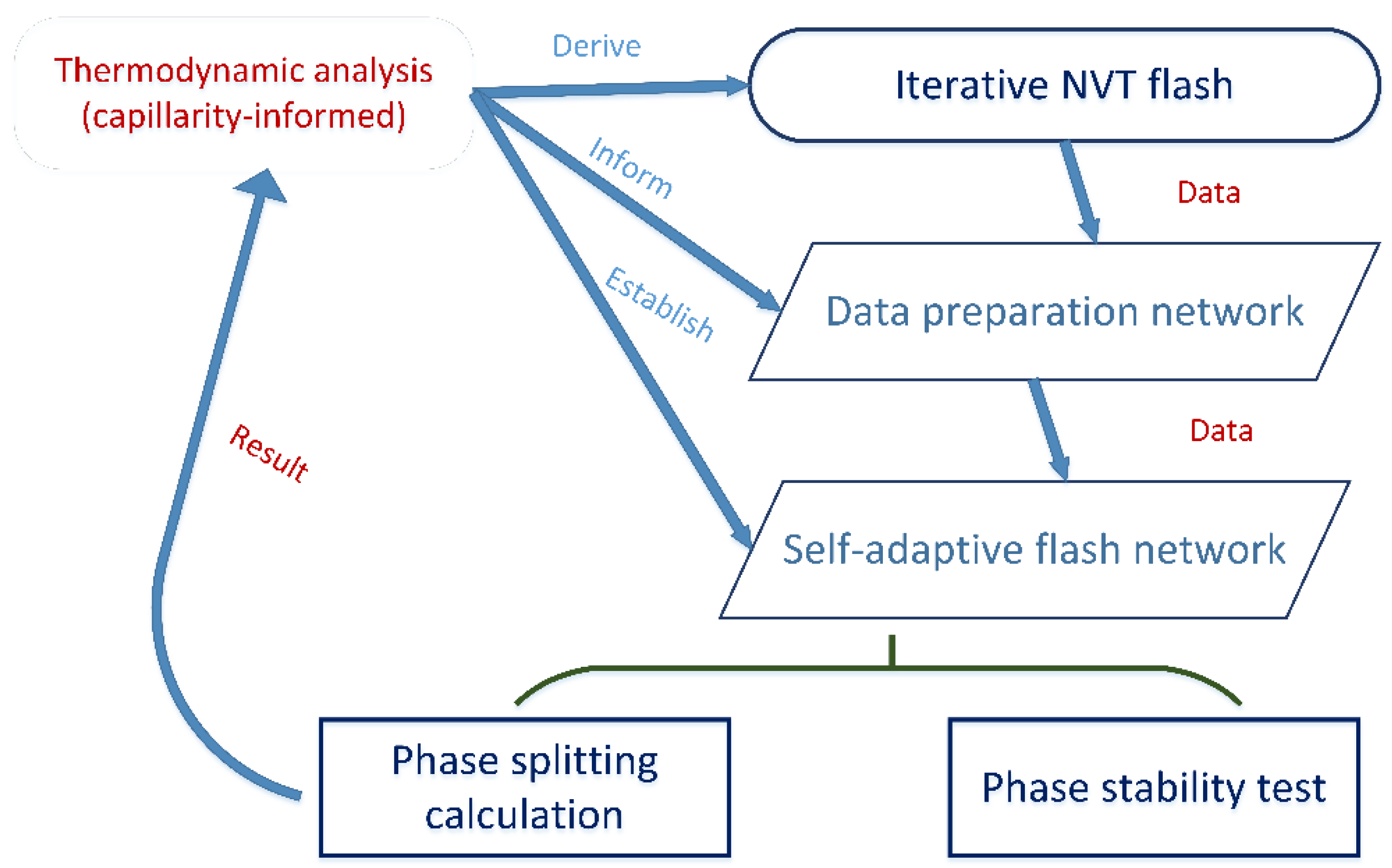
In order to overcome the limitations of the current phase equilibrium calculation methods and the accelerated approach using the deep learning technique, a thermodynamically consistent phase equilibrium calculation scheme is proposed in this paper, as shown in Figure 1. This work starts from the realistic equation of state and a thermodynamically consistent NVT type flash calculation method is generated as discussed in Section 2. Using iterative calculations, sufficient data can be prepared for the further training and testing purposed in the deep learning algorithm, and the network structure is also designed based on thermodynamic analysis to determine the input and output features. A two-network structure is established for the adaptive flash calculation, with one network for data padding and the other one for phase equilibrium prediction. Both phase stability test and phase splitting calculations are involved in the output of the flash network, which informs both the number of phases at equilibrium and the compositional mole fraction. The predictions can be further analyzed using the thermodynamic scheme. As illustrated in the figure, data are transferred through both the iterative flash calculation scheme and the accelerated deep learning scheme, and thermodynamic analysis plays a role in the whole process. Such a coherent and complete phase equilibrium calculation scheme is believed to be capable of providing fast, accurate and robust thermodynamic foundations for further multi-component multi-phase fluid flow simulation [39]. It should also be noticed that the thermodynamic correlations among the input features are now described by the inner connections of the hidden layers and nodes, as well as the usage of activation functions, to replace the conventional thermodynamic models represented by EOSs. If the trained model as a liner combination of the nodes and activation functions is verified to meet well with the ground truth data, i.e., iterative flash calculation data in a wide range of environmental conditions, it is reasonable to state that the thermodynamic rules in the phase equilibrium calculations are well-informed in the proposed deep neural network.
For oil and gas reservoirs, hydrocarbons are considered to be the main components existing in the investigated fluid mixtures. Peng–Robinosn EOS [40] is proven to be a good one describing the thermodynamic properties of hydrocarbons, which could be formulated in a polynomial form as:
where the parameters and can be calculated as:
The pressure correction coefficient and volume correction coefficient can be calculated by:
where the attraction parameter is modeled by:
We define the acentric factor as a conceptual number to be a measure of the non-sphericity (centricity) of molecules. As it increases, the vapor curve is “pulled” down, resulting in higher boiling points. The coefficient in Equation (17) can be calcualted by for . If holds, then the coefficient should be determiend based on .
Based on the previous thermodynamic analysis, the critical temperature , critical pressure and acentric factor are chosen to be the key features identifying each component , while the mole fraction is also needed as an initial condition. For an NVT type flash calculation, environmental temperature and overall molar concentration are slected to be the environmental conditions, and the pore size should also be included to involve the effect of capillarity in general reservoir geometries. Thus, the dimension of the input data is for the input fluid mixture with components. The data prepartion network will read the number of components of the target fluid and automatically construct the output layer with a dimension of , while can be different from . If , all information in the training data will be retained, and data padding will be carried out by defining the ghost components with all the key thermodynamic characteristics set as zero. The result data output by this network have a dimension of . If , the data set output by this network remains the same as the input training data, but the test data set of the target fluid is filled with ghost components with zero key thermodynamic characteristics. In this way, it can be ensured that the input and output data dimensions of the second neural network, that is, the self-adaptive flash network plotted in Figure 1, are the same, thereby realizing the wide applicability of phase equilibrium calculations for practical reservoir fluids including unconventional reservoirs, with variable compositions and capillary pressures.
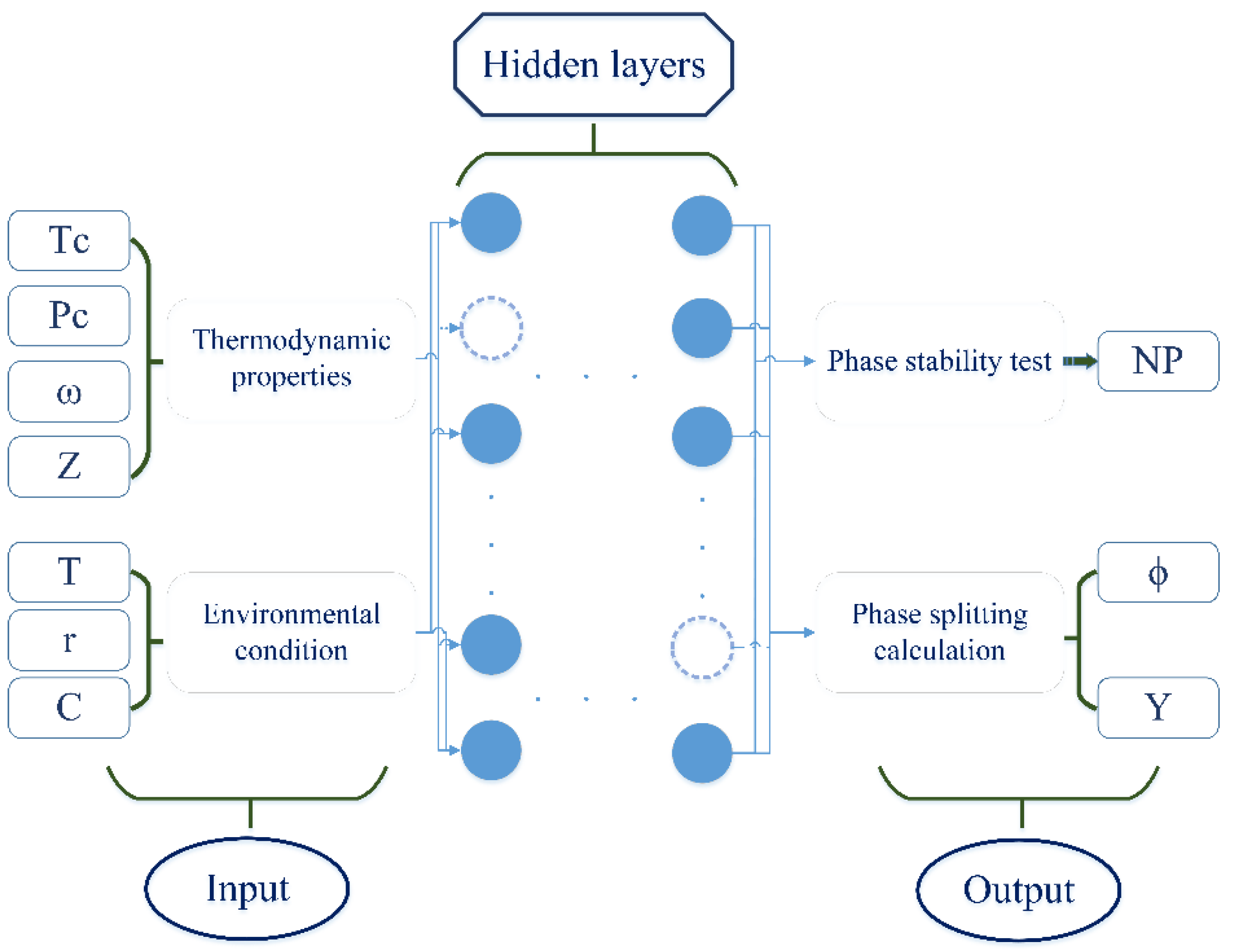
The structure of the flash neural network is illustrated in Figure 2. The output layer will obtain the result of the phase stability test, that is, the total number of phases in the fluid at the equilibrium state, represented by , and the result of the phase splitting calculation, that is, the molar composition of the gas phase () and the gas–liquid ratio () at the equilibrium state. A number of hidden layers are placed between the input and output layer [41]. Each hidden layer contains several nodes, and the model trained on each layer can be expressed as:
where denotes the weight parameters in the th hidden layer, denotes the input data in that layer and denotes the output data. represents the activation function used in that layer, and is the bias. For a fully connected deep neural network, the output data from the previous layer are usually directly used as the input data of the next layer. Taking a neural network consisting of three hidden layers as an example, the overall prediction model is:
where denotes the final output predictions, denotes the input data in the first layer, , and denote the weight parameter in the 1st, 2nd and 3rd layer, respectively, and , and denote the activation functions used in the layers.
The self-adaptive neural network architecture proposed in this paper will allow the data to be padded to unify the training data set and the target test data set, which brings the following corrections to the above training model: assuming , the ghost components are defined with zero key thermodynamic properties and padded into the input data, which could be formulated as:
where the subscript denotes the ghost components.
Overfitting is a common challenge in deep learning research, which means that the perfect performance of the trained model has been achieved for training data, but only poor performance can be obtained when verifying the predictions for the testing data. Usually, this problem occurs if too many parameters are included in a deep learning model (also known as an over-parameterized model). For multi-component phase equilibrium problems, the calculation model generally includes a super-large-scale weight matrix, especially when the realistic oil and gas reservoir fluid, containing a large number of components, is taken into account. An additional constraint is usually applied to reduce the degree of freedom of the model to prevent overfitting from damaging the performance of the deep learning algorithm. An important feature of overfitting is that the norm of the coefficient parameter is very large, which may help us point out a solution to add this additional constraint. The loss function could be corrected by adding a L2 norm of weight matrix, which may help avoid the extra-large weight matrix in the final trained model.
The super-large-scale weight matrix needed by the phase equilibrium prediction model of realistic multi-component oil and gas reservoir fluids requires a good initial guess to improve the convergence speed during training, thereby improving the performance and reliability of the developed deep learning algorithms. If the weight parameters are overestimated in the initialization, a rapid increase in variance may be observed during the training process, which may further cause the gradient to explode or disappear. In this case, the training will never converge. On the contrary, if the weight parameters are underestimated during initialization, the variance may quickly drop to a very small value, which will lead to the loss of model complexity and even damage the performance of the final evaluation. The commonly used initialization method is to initialize the weight parameters with a certain variance following the Gaussian distribution to ensure that the input and output variances of each layer will remain unchanged. This is the commonly used Xavier initialization technique [44], which is also used in this paper to initialize the weight matrix predicting the phase equilibrium.
In order to accurately describe the complex thermodynamic laws in the phase equilibrium investigations, it is difficult for the model trained by the deep neural network to fully avoid the overfitting problem caused by the high complexity, which affects the final prediction effect. Dropout is a common method that eliminates the corresponding connections by discarding certain nodes in the network, thereby significantly reducing the degree of freedom of the model. As shown in Figure 2, the dotted circle in the hidden layer represents the node eliminated by the dropout technique. After evaluating all nodes and connections with certain probability, the training of the model will be performed on the simplified network after dropout. It should be pointed out that in order to maintain the robustness of training and conservation of the physical laws, before the start of the next training cycle, it is necessary to use the initialized coefficients to insert the discarded nodes back into the model for re-evaluation and dropout operations.
Due to the complexity of the multi-component phase equilibrium prediction model and the huge amount of training data required, the training of the deep learning model is very time-consuming. In addition, together with the gradient descent process, the variable matrix and of each layer may change, which in turn causes the linear and nonlinear calculation result distribution of each layer to change frequently. The next layer in the network has to constantly adapt to this distribution change, which will make the learning rate of the entire network too slow. In addition, when using saturated activation functions, such as sigmoid, tanh, etc., it is easy to cause the model training to fall into the gradient saturation zone. At this time, the gradient will become very small or even close to 0, and the update speed of the parameters will slow down, which further slows down the convergence rate of the network training. This is the common internal covariate shift problem (Internal Covariate Shift, ICS) in machine learning. A usual solution is whitening, that is, making the input feature distribution to have the same mean and variance, thereby reducing the impact of the ICS problem. However, the computational cost of the whitening technique is too high, especially when every layer in each round of training needs to perform this operation, which slows down the training efficiency. In addition, because the whitening process changes the distribution of each layer of the network, it changes the expressive ability of the raw data in the network configurations. It is often questioned that certain information underlying the physical rules among the input features may be lost after whitening process, so that the trained model cannot be trusted for the accurate and robust predictions with physical meanings. Therefore, a more advanced batch normalization method (Batch Normalization, BN [45]) is used in this paper to calculate the mean and variance for each batch of data samples, and then standardizes the distribution of each input feature values with a mean value of 0 and a variance of 1. Linear transformations are also added to recover the information underneath the input data.
The strong nonlinear correlations among the input features (characterized by the nonlinear evolution equations based on the equation of state in conventional iterative flash calculation) is characterized by the activation functions in the deep learning model. As a key factor in expressing network nonlinearity and problem-solving ability, the activation function has developed rapidly in recent years. Different activation functions have different expressions and thus are preferred in different engineering scenarios. In previous publications, careful tuning has been carried out on the selection of the best activation function for phase equilibrium prediction, and generally “softsign” function performs the best. In addition, the “softmax” function, formulated as:
should also be included in the last layer. By calculating the ratio of the index of the mole fraction of each component in each phase to the sum of the index of the mole fraction of all components in that phase, it can be ensured that the final output of the deep neural network meets the restriction condition that the sum of mole fractions in each phase is 1, so as to preserve the consistency and physical meanings of thermodynamics.
4. Results
4.1. Scheme Verification
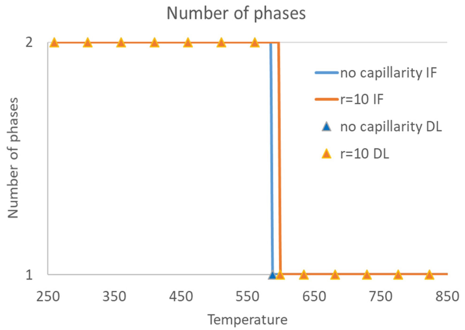
The number of phases existing in the mixture at the phase equilibrium state is the most critical information for multi-phase fluid flow problems, as it can be directly used to determine whether the simulation settlement of multi-phase flow is needed or a simple single-phase flow model is enough for the case. One important contribution of the proposed deep learning algorithm is to incorporate the phase stability test and phase splitting calculation as the output and directly predict the number of phases at equilibrium in the final output layer. Under the condition of a constant molar concentration of 189.85 mol/m3, total number of phases of the eight-component Eagle Ford oil fluid mixture at different temperatures at the equilibrium state is plotted in Figure 3. Details of the thermodynamic properties used for each component is referred from [35] and the network architecture can be referred from [36]. As shown clearly in the plot, the trained model using our proposed network configuration and algorithm can predict well on the phase stability test, while the deep learning results (represented by DL and plotted by triangles) meet well with the ground truth data, i.e., the iterative flash calculation results (represented by IF and plotted by lines). Phase transitions can be perfectly captured using the trained model, thus, we can determine when to use the single-phase model and when to use the multi-phase model for efficient and reliable flow simulations.
The effect of capillarity can also be detected in Figure 3. It can be easily referred that the two-phase region has been extended if capillarity is taken into account, while a higher temperature is needed for the mixture entering the single (vapor) phase region. This finding meets exactly the conclusion in [37] that the bubble point curve is suppressed with capillarity while the dew point curve is expanded outward with dew point pressure decreasing (and increasing) in the lower (and upper) branch of the dew point curve in the phase envelop. Thus, the proposed TINN configuration is proven to be effective in both phase equilibrium predictions and study on the effect capillary pressures.
4.2. Prediction Considering Various Capillarity
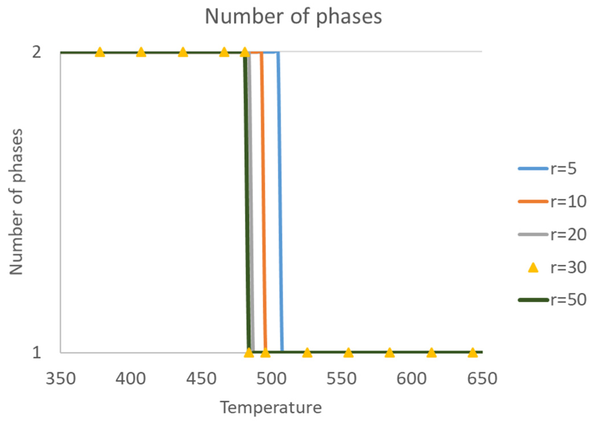
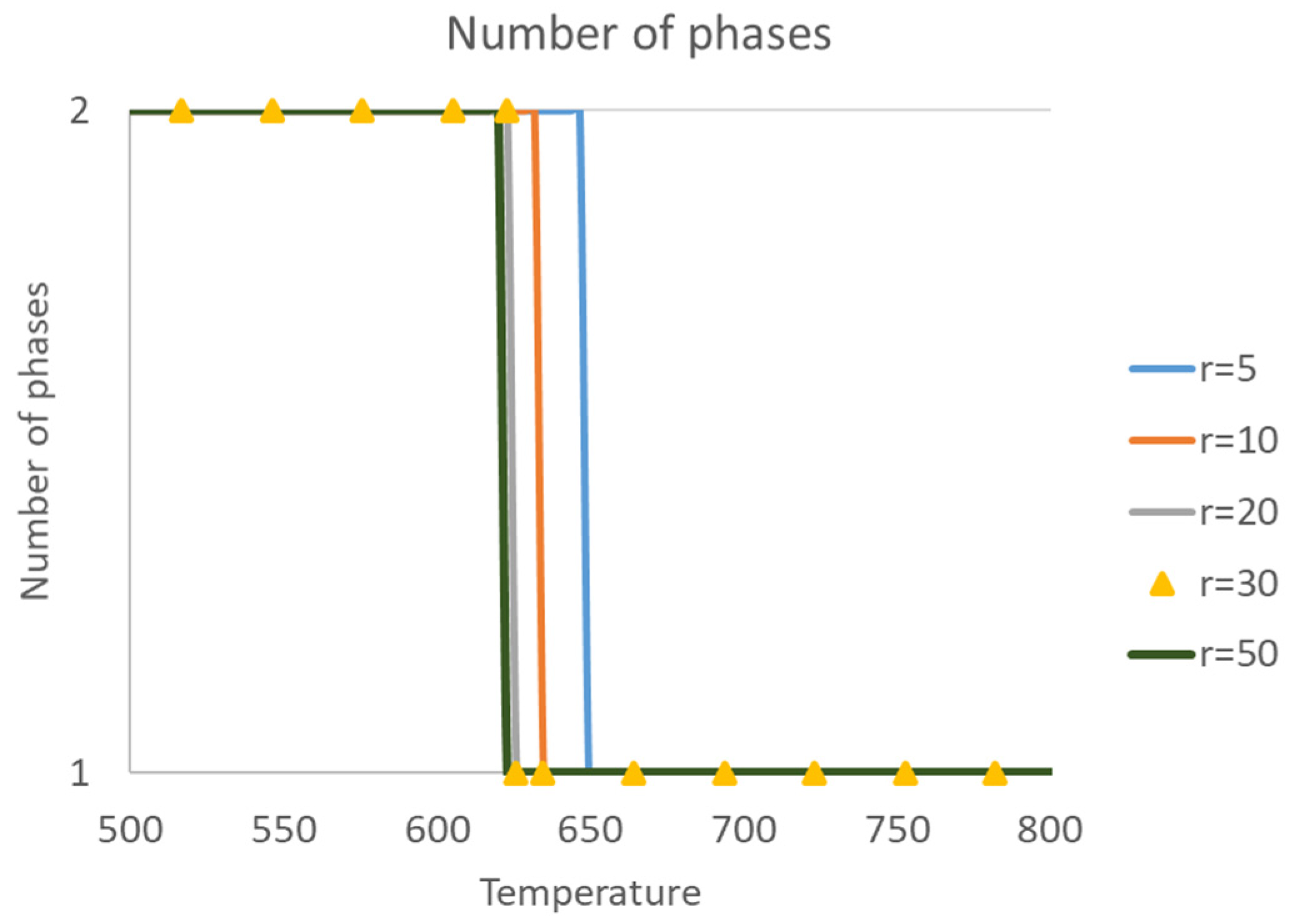
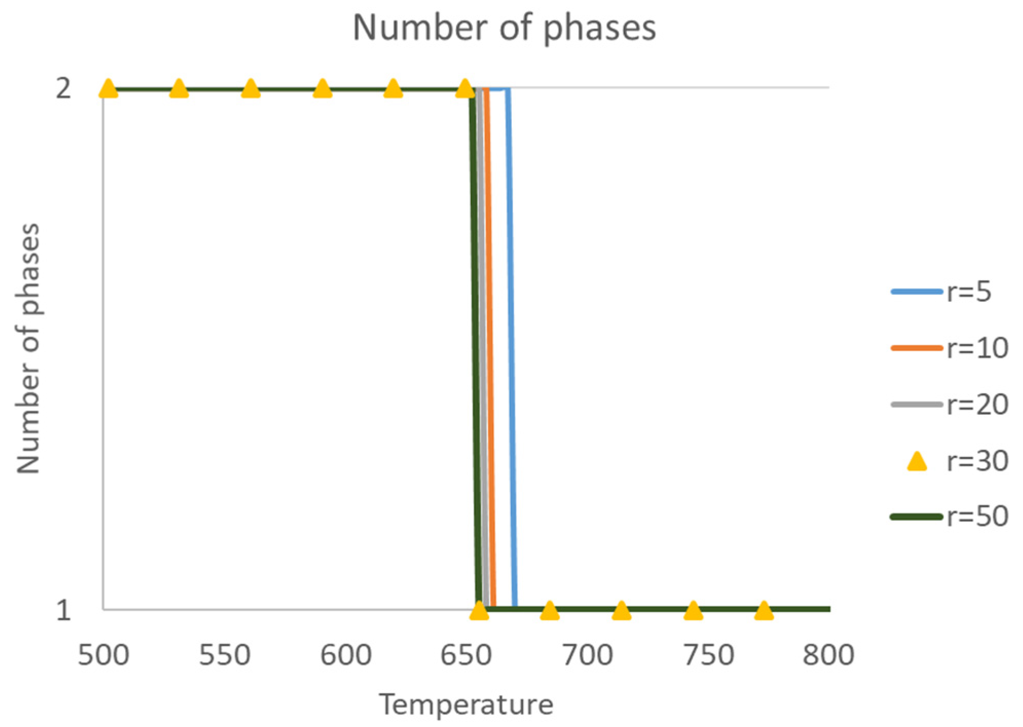
One significant contribution of this paper is the general adaptability on various capillarity with changing pore sizes. The phase stability test result for the eight-component Eagle Ford Oil fluid mixture in the pore size distribution of 5, 10, 20, 30 and 50 is plotted in Figure 4, Figure 5 and Figure 6 under the constant overall mole concentration as 10 mol/m3, 429.65 mol/m3 and 1568.7 mol/m3, respectively. It can be found in the illustrations that the phase transitions point varies with different pore size distributions, and generally, a larger pore size may result in a lower phase transition temperature. Considering the effect of capillarity studied in the previous section, it can be further referred that the impact of capillary pressure on the phase equilibrium conditions increases with smaller pore size distributions, which is consistent with the general assumption that the capillary effect is less important in large pores. Moreover, the capillary effect on the phase stability test may be the same even if the pore size distributions change a little bit.
It should also be pointed out that self-adaptive deep learning technique is also verified in this work, as we use the five-component Bakken Oil fluid data as the input, and the data padding of three ghost components are defined to uniform the data size. The effective training and accurate prediction validate the idea of self-adaptive deep learning and the data padding method with ghost components.
It can also be found by comparisons among the three figures that the phase transitions temperature increases with higher overall mole concentrations, which enlarges the two-phase region. This finding is consistent with the general rule that a higher mole concentration can help liquefaction under the same other environmental conditions, thus further verifying the thermodynamic consistency and physical meanings of our proposed deep learning scheme. From another viewpoint, a higher overall mole concentration is equivalent to a higher molecular density in the domain thanks to the conservation of moles, which further results in a higher thermodynamic pressure. Moreover, the effect of capillary pressure on the phase transitions decreases with a higher overall mole concentration, as the temperature difference on the phase transitions is narrowed.
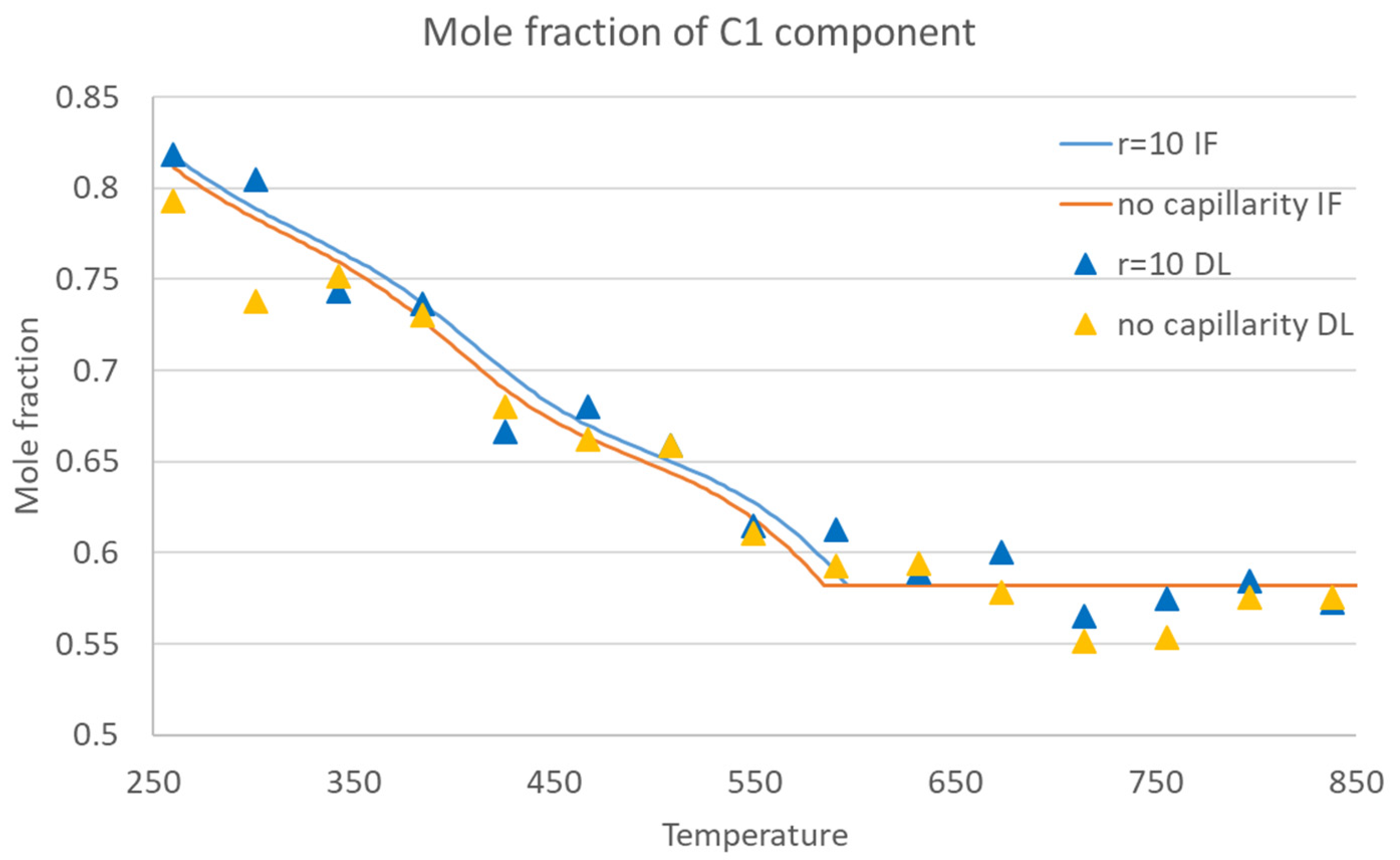
Except for the phase stability test, the phase splitting calculation is also needed prior to the multi-component multi-phase flow simulation, to provide thermodynamically consistent initial compositional phase distributions. The deep learning predictions on the phase splitting calculations are illustrated in Figure 7 and Figure 8, taking the mole fractions of C1 component in the vapor phase and the C7+ component in the liquid phase as the example, respectively. The accuracy of the trained deep learning model has been verified again by the acceptable variance from the ground truth data. It can also be referred from the plotting that the compositional phase distributions change with the increasing temperature, while only the vapor phase can be detected in the mixture at equilibrium above certain temperatures. This capture of phase transitions meets well with the previous finding on the phase stability test, as shown in Figure 3. Meanwhile, the effect of capillarity can also be detected on both the phase transitions and compositional distributions, and it is proven again that the consideration of capillarity may result in a larger two-phase region as a higher phase transition temperature is needed.
Improving the computational efficiency is always the main reason of using deep learning techniques. As shown in Table 1, the phase equilibrium prediction using the proposed deep learning algorithm has been significantly accelerated compared with the conventional iterative NVT flash calculation method. Thus, the proposed scheme in this paper is proven to be fast.
5. Discussion and Concluding Remarks
In order to better predict the phase equilibrium conditions in unconventional oil and gas exploration and development, which is a key issue related to the reliability and physical consistency of multi-component multi-phase flow simulation in subsurface porous media, a thermodynamically consistent NVT type flash calculation method is developed based on the realistic equation of state, starting from the first and second law of thermodynamics. The key features in the phase equilibrium process are extracted based on the thermodynamic analysis, and a deep learning algorithm is developed to accelerate the phase equilibrium predictions of multi-component fluid systems. A two-network structure is proposed to extend the adaptability to general reservoir fluids consisting of different number of components under a wide range of environmental conditions. The self-adaptability of the proposed scheme is verified by a good prediction of eight-component Eagle Ford Oil using the training data of five-component Bakken Oil, with three ghost components defined and padded. The scheme is proven to be fast, accurate and robust by comparisons with the conventional iterative flash calculation method in various cases, and both the phase stability test and the phase splitting calculation are incorporated well in the reliable outputs. The effect of capillarity can be captured in both the number of phases existing at equilibrium and the compositional phase distributions. Generally, a higher temperature is needed to change from the two-phase region to the single-vapor-phase region if capillarity is taken into account. Moreover, the capillary effect is more obvious if a lesser pore size distribution is involved.
Thermodynamics have been informed in both the data preparation using iterative flash calculation and determination of the network configurations. The good prediction performance further validates that the thermodynamic rules governing phase equilibrium problems are now recovered well using the trained model as a combination of the many weights and activation functions in the hidden nodes. It should also be noted that although iterative flash calculation data are used for data preparation in this paper, experimental data are always preferred. In fact, the EOSs, as the foundation of both NPT and NVT flash schemes, are generally analyzed and regressed from experimental data. Thus, the trained model is expected to be more reliable if directly learned from the experimental data. However, it is extremely hard and expensive to carry out phase equilibrium experiments, especially for complex realistic reservoir fluids consisting of a large number of components and under a wide range of environmental conditions.
Author Contributions
Conceptualization, S.S.; methodology, T.Z.; software, T.Z..; validation, S.S., T.Z.; writing—original draft preparation, T.Z.; writing—review and editing, S.S. All authors have read and agreed to the published version of the manuscript.
Funding
The authors greatly thank the support from the Research Funding from King Abdullah University of Science and Technology (KAUST) through the grant BAS/1/1351-01-01.
Institutional Review Board Statement
Not applicable.
Informed Consent Statement
Not applicable.
Data Availability Statement
Not applicable.
Conflicts of Interest
The authors declare no conflict of interest.
Nomenclature
| Symbol | Meaning |
| Helmholtz free energy | |
| Volume-averaged energy density | |
| Gas phase | |
| Liquid phase | |
| Volume | |
| Molar density vector | |
| Component index | |
| Diffusion coefficient | |
| Capillary pressure | |
| Interfacial tension | |
| Onsager coefficients | |
| Pore size | |
| Acentric factor | |
| Pressure correction coefficient | |
| Volume correction coefficient |
References
- Qyyum, M.A.; Chaniago, Y.D.; Ali, W.; Qadeer, K.; Lee, M. Coal to clean energy: Energy-efficient single-loop mixed-refrigerant-based schemes for the liquefaction of synthetic natural gas. J. Clean. Prod. 2019, 211, 574–589. [Google Scholar] [CrossRef]
- Woollacott, J. A bridge too far? The role of natural gas electricity generation in US climate policy. Energy Policy 2020, 147, 111867. [Google Scholar] [CrossRef]
- Shen, Y.; Ge, H.; Zhang, X.; Chang, L.; Liu, D.; Liu, J. Impact of fracturing liquid absorption on the production and water-block unlocking for shale gas reservoir. Adv. Geo-Energy Res. 2018, 2, 163–172. [Google Scholar] [CrossRef] [Green Version]
- Zhang, T.; Li, Y.; Sun, S. Phase equilibrium calculations in shale gas reservoirs. Capilarity 2019, 2, 8–16. [Google Scholar] [CrossRef] [Green Version]
- Wang, H.; Chen, L.; Qu, Z.; Yin, Y.; Kang, Q.; Yu, B.; Tao, W.-Q. Modeling of multi-scale transport phenomena in shale gas production—A critical review. Appl. Energy 2020, 262, 114575. [Google Scholar] [CrossRef]
- Chen, L.; Zuo, L.; Jiang, Z.; Jiang, S.; Liu, K.; Tan, J.; Zhang, L. Mechanisms of shale gas adsorption: Evidence from thermodynamics and kinetics study of methane adsorption on shale. Chem. Eng. J. 2019, 361, 559–570. [Google Scholar] [CrossRef]
- Huai, J.; Xie, Z.; Li, Z.; Lou, G.; Zhang, J.; Kou, J.; Zhao, H. Displacement behavior of methane in organic nanochannels in aqueous environment. Capillarity 2020, 3, 56–61. [Google Scholar] [CrossRef]
- Jimenez, B.A.L.; Hernandez, G.; Czernia, B.; Killough, J.E.; Barrufet, M.A. Effects of Thermodynamic and Rock Properties on the Performance of Liquids-Rich Nano-Porous Shale Reservoirs. In Proceedings of the Day 1 Tue, SPE Argentina Exploration and Production of Unconventional Resources Symposium, Neuquén, Argentina, 14–16 August 2018. [Google Scholar]
- Wang, S.; Sobecki, N.; Ding, D.; Wu, Y.-S.; Zhu, L. Accelerated Compositional Simulation of Tight Oil and Shale Gas Reservoirs Using Proxy Flash Calculation. In Proceedings of the Day 1 Wed, SPE Reservoir Simulation Conference, OnePetro, Galveston, TX, USA, 10–11 April 2019. [Google Scholar]
- Slattery, J.C. Single-phase flow through porous media. AIChE J. 1969, 15, 866–872. [Google Scholar] [CrossRef]
- Paulaitis, M.E.; Krukonis, V.J.; Kurnik, R.T.; Reid, R.C. Supercritical fluid extraction. Rev. Chem. Eng. 1983, 1, 179–250. [Google Scholar]
- Whitson, C.H.; Michelsen, M.L. The negative flash. Fluid Phase Equil. 1989, 53, 51–71. [Google Scholar] [CrossRef]
- Sobecki, N.; Nieto-Draghi, C.; Di Lella, A.; Ding, D.Y. Phase behavior of hydrocarbons in nanopores. Fluid Phase Equil. 2019, 497, 104–121. [Google Scholar] [CrossRef]
- Bi, R.; Firoozabadi, A.; Myint, P.C. Efficient and robust phase-split computations in the internal energy, volume, and moles (UVN) space. Fluid Phase Equil. 2020, 526, 112729. [Google Scholar] [CrossRef]
- Sandoval, D.R.; Michelsen, M.L.; Yan, W.; Stenby, E.H. VT-based phase envelope and flash calculations in the presence of capillary pressure. Ind. Eng. Chem. Res. 2019, 58, 5291–5300. [Google Scholar] [CrossRef] [Green Version]
- Luo, S.; Lutkenhaus, J.L.; Nasrabadi, H. Multiscale Fluid-Phase-Behavior Simulation in Shale Reservoirs Using a Pore-Size-Dependent Equation of State. SPE Reserv. Eval. Eng. 2018, 21, 806–820. [Google Scholar] [CrossRef]
- Huo, S.; Jiao, K.; Park, J.W. On the water transport behavior and phase transition mechanisms in cold start operation of PEM fuel cell. Appl. Energy 2019, 233–234, 776–788. [Google Scholar] [CrossRef]
- Wu, S.; Li, Z.; Sarma, H.K. Influence of confinement effect on recovery mechanisms of CO2-enhanced tight-oil recovery process considering critical properties shift, capillarity and adsorption. Fuel 2020, 262, 116569. [Google Scholar] [CrossRef]
- Van der Waals, J.H. On the Continuity of the Gases and Liquid State. Doctoral Dissertation, Leiden University, Leiden, The Netherlands, 1873. [Google Scholar]
- Baled, H.; Enick, R.M.; Wu, Y.; McHugh, M.A.; Burgess, W.; Tapriyal, D.; Morreale, B.D. Prediction of hydrocarbon densities at extreme conditions using volume-translated SRK and PR equations of state fit to high temperature, high pressure PVT data. Fluid Phase Equil. 2012, 317, 65–76. [Google Scholar] [CrossRef]
- Sanchez-Rivera, D.; Mohanty, K.; Balhoff, M. Reservoir simulation and optimization of Huff-and-Puff operations in the Bakken Shale. Fuel 2015, 147, 82–94. [Google Scholar] [CrossRef]
- Michelsen, M.L. Simplified flash calculations for Cubic Equations of State. Ind. Eng. Chem. Process. Des. Dev. 1986, 25, 184–188. [Google Scholar] [CrossRef]
- Jensen, B.H.; Aage, F. A simplified flash procedure for multicomponent mixtures containing hydro-carbons and one non-hydrocarbon using two-parameter cubic equations of state. Ind. Eng. Chem. Res. 1987, 26, 2129–2134. [Google Scholar]
- Hendriks, E.M. Reduction theorem for phase equilibrium problems. Ind. Eng. Chem. Res. 1988, 27, 1728–1732. [Google Scholar] [CrossRef]
- Firoozabadi, A.; Pan, H. Fast and Robust Algorithm for Compositional Modeling: Part I—Stability Analysis Testing. SPE J. 2002, 7, 78–89. [Google Scholar] [CrossRef] [Green Version]
- Li, Y.; Johns, R.T. Rapid Flash Calculations for Compositional Simulation. SPE Reserv. Eval. Eng. 2006, 9, 521–529. [Google Scholar] [CrossRef]
- Nichita, D.V.; Petitfrere, M. Phase stability analysis using a reduction method. Fluid Phase Equil. 2013, 358, 27–39. [Google Scholar] [CrossRef]
- Gaganis, V. Rapid phase stability calculations in fluid flow simulation using simple discriminating functions. Comput. Chem. Eng. 2018, 108, 112–127. [Google Scholar] [CrossRef]
- Petitfrere, M.; Nichita, D.V. A comparison of conventional and reduction approaches for phase equilibrium calculations. Fluid Phase Equil. 2015, 386, 30–46. [Google Scholar] [CrossRef]
- Alom, M.Z.; Taha, T.M.; Yakopcic, C.; Westberg, S.; Sidike, P.; Nasrin, M.S.; Asari, V.K. The history began from alexnet: A comprehensive survey on deep learning approaches. arXiv 2018, arXiv:1803.01164. [Google Scholar]
- Voulodimos, A.; Doulamis, N.; Doulamis, A.; Protopapadakis, E. Deep Learning for Computer Vision: A Brief Review. Comput. Intell. Neurosci. 2018, 2018, 7068349. [Google Scholar] [CrossRef]
- Young, T.; Hazarika, D.; Poria, S.; Cambria, E. Recent Trends in Deep Learning Based Natural Language Processing. IEEE Comput. Intell. Mag. 2018, 13, 55–75. [Google Scholar] [CrossRef]
- Skinner, G.; Walmsley, T. Artificial Intelligence and Deep Learning in Video Games A Brief Review. In Proceedings of the 2019 IEEE 4th International Conference on Computer and Communication Systems (ICCCS), Singapore, 23–25 February 2019; pp. 404–408. [Google Scholar]
- Li, Y.; Zhang, T.; Sun, S.; Gao, X. Accelerating flash calculation through deep learning methods. J. Comput. Phys. 2019, 394, 153–165. [Google Scholar] [CrossRef] [Green Version]
- Li, Y.; Zhang, T.; Sun, S. Acceleration of the NVT Flash Calculation for Multicomponent Mixtures Using Deep Neural Network Models. Ind. Eng. Chem. Res. 2019, 58, 12312–12322. [Google Scholar] [CrossRef] [Green Version]
- Zhang, T.; Li, Y.; Li, Y.; Sun, S.; Gao, X. A self-adaptive deep learning algorithm for accelerating multi-component flash calculation. Comput. Methods Appl. Mech. Eng. 2020, 369, 113207. [Google Scholar] [CrossRef]
- Zhang, T.; Li, Y.; Sun, S.; Bai, H. Accelerating flash calculations in unconventional reservoirs considering capillary pressure using an optimized deep learning algorithm. J. Pet. Sci. Eng. 2020, 195, 107886. [Google Scholar] [CrossRef]
- Weinaug, C.F.; Katz, D.L. Surface Tensions of Methane-Propane Mixtures. Ind. Eng. Chem. 1943, 35, 239–246. [Google Scholar] [CrossRef]
- Garg, S.; Shariff, A.M.; Shaikh, M.; Lal, B.; Suleman, H.; Faiqa, N. Experimental data, thermodynamic and neural network modeling of CO2 solubility in aqueous sodium salt of l-phenylalanine. J. CO2 Util. 2017, 19, 146–156. [Google Scholar] [CrossRef]
- ZareNezhad, B.; Eggeman, T. Application of Peng–Rabinson equation of state for CO2 freezing prediction of hydrocarbon mixtures at cryogenic conditions of gas plants. Cryogenics 2006, 46, 840–845. [Google Scholar] [CrossRef]
- Haykin, S. Neural Networks and Learning Machines, 3/E; Pearson Education India: London, UK, 2010. [Google Scholar]
- Poort, J.P.; Ramdin, M.; van Kranendonk, J.; Vlugt, T.J. Solving vapor-liquid flash problems using artificial neural networks. Fluid Phase Equil. 2019, 490, 39–47. [Google Scholar] [CrossRef] [Green Version]
- Wang, S.; Sobecki, N.; Ding, D.; Zhu, L.; Wu, Y.-S. Accelerating and stabilizing the vaporliquid equilibrium (VLE) calculation in compositional simulation of unconventional reservoirs using deep learning based flash calculation. Fuel 2019, 253, 209–219. [Google Scholar] [CrossRef]
- Koturwar, S.; Merchant, S. Weight initialization of deep neural networks (DNNs) using data statistics. arXiv 2017, arXiv:1710.10570. [Google Scholar]
- Santurkar, S.; Tsipras, D.; Ilyas, A.; Mądry, A. How does batch normalization help optimization? In Proceedings of the 32nd International Conference on Neural Information Processing Systems, Montreal, QC, Canada, 2–8 December 2018; pp. 2488–2498. [Google Scholar]
- Haykin, S. Neural Networks and Learning Machines; Pearson: Upper Saddle River, FL, USA, 2009. [Google Scholar]
Figure 1.
Structure of the thermodynamically consistent phase equilibrium calculation scheme considering capillarity.
Figure 1.
Structure of the thermodynamically consistent phase equilibrium calculation scheme considering capillarity.

Figure 2.
Schematic diagram of the flash neural network considering capillarity.

Figure 3.
Number of phases at equilibrium changing with temperature under the constant overall mole concentration as 189.85 mol/m3.
Figure 3.
Number of phases at equilibrium changing with temperature under the constant overall mole concentration as 189.85 mol/m3.

Figure 4.
Number of phases at equilibrium changing with temperature under the constant overall mole concentration as 10 mol/m3.
Figure 4.
Number of phases at equilibrium changing with temperature under the constant overall mole concentration as 10 mol/m3.

Figure 5.
Number of phases at equilibrium changing with temperature under the constant overall mole concentration as 429.65 mol/m3.
Figure 5.
Number of phases at equilibrium changing with temperature under the constant overall mole concentration as 429.65 mol/m3.

Figure 6.
Number of phases at equilibrium changing with temperature under the constant overall mole concentration as 1568.7 mol/m3.
Figure 6.
Number of phases at equilibrium changing with temperature under the constant overall mole concentration as 1568.7 mol/m3.

Figure 7.
Mole fractions of C1 component in the vapor phase changing with temperature under the constant overall mole concentration as 189.85 mol/m3.
Figure 7.
Mole fractions of C1 component in the vapor phase changing with temperature under the constant overall mole concentration as 189.85 mol/m3.

Figure 8.
Mole fractions of C7+ component in the liquid phase changing with temperature under the constant overall mole concentration as 189.85 mol/m3.
Figure 8.
Mole fractions of C7+ component in the liquid phase changing with temperature under the constant overall mole concentration as 189.85 mol/m3.


Table 1.
Comparison between the CPU time used for iterative flash calculation and deep learning accelerated algorithm.
Table 1.
Comparison between the CPU time used for iterative flash calculation and deep learning accelerated algorithm.
| Method | CPU Time (s) | Acceleration |
|---|---|---|
| Iterative NVT flash | 933 | NA |
| Deep learning algorithm | 3.2 | 291.56 |
Publisher’s Note: MDPI stays neutral with regard to jurisdictional claims in published maps and institutional affiliations. |
© 2021 by the authors. Licensee MDPI, Basel, Switzerland. This article is an open access article distributed under the terms and conditions of the Creative Commons Attribution (CC BY) license (https://creativecommons.org/licenses/by/4.0/).
Share and Cite
MDPI and ACS Style
Zhang, T.; Sun, S. Thermodynamics-Informed Neural Network (TINN) for Phase Equilibrium Calculations Considering Capillary Pressure. Energies 2021, 14, 7724. https://0-doi-org.brum.beds.ac.uk/10.3390/en14227724
AMA Style
Zhang T, Sun S. Thermodynamics-Informed Neural Network (TINN) for Phase Equilibrium Calculations Considering Capillary Pressure. Energies. 2021; 14(22):7724. https://0-doi-org.brum.beds.ac.uk/10.3390/en14227724
Chicago/Turabian StyleZhang, Tao, and Shuyu Sun. 2021. "Thermodynamics-Informed Neural Network (TINN) for Phase Equilibrium Calculations Considering Capillary Pressure" Energies 14, no. 22: 7724. https://0-doi-org.brum.beds.ac.uk/10.3390/en14227724
Note that from the first issue of 2016, this journal uses article numbers instead of page numbers. See further details here.