Direct Fuzzy CMAC Sliding Mode Trajectory Tracking for Biaxial Position System

Abstract

High-precision trajectory control is considered as an important factor in the performance of industrial two-axis contour motion systems. This research presents an adaptive direct fuzzy cerebellar model articulation controller (CMAC) sliding mode control (DFCMACSMC) for the precise control of the industrial XY-axis motion system. The FCMAC was utilized to approximate an ideal controller, and the weights of FCMAC were on-line tuned by the derived adaptive law based on the Lyapunov criterion. With this derivation in mind, the asymptotic stability of the developed motion system could be guaranteed. The two-axis stage system was experimentally investigated using four contours, namely, circle, bowknot, heart, and star reference contours. The experimental results indicate that the proposed DFCMACSMC method achieved the improved tracking capability, and so reveal that the DFCMACSMC scheme outperformed other schemes of the model uncertainties and cross-coupling interference.

1. Introduction

Precision motion systems are being used extensively in precision fields, such as computer numerical control (CNC) machineries, IC manufacturing, micro-mechanical assembly, ultraprecision measurement, and microsurgery. Machine systems are generally designed to reduce tracking errors with respect to each feed drive axis.

The micro-meter level system is becoming increasingly important in satisfying the requirements for mass production in industrial 4.0. The permanent magnet synchronous motor (PMSM) [1,2,3,4,5] is a device designed by using permanent magnets embedded in the steel rotor to create a constant magnetic field. It provides for several better properties, including low torque ripple, high efficiency, high power density, low maintenance cost, low heat generation, and so forth. However, it still has some inherent disadvantages, such as complex control systems, higher cost, and low reliability. Moreover, the servo-performance of the biaxial motion control system is affected by backlash, nonlinear friction characteristics, unmodeled dynamics, and other time-varying conditions. To better compensate these uncertainties and nonlinearities, a better control scheme should be used for motion control systems.

Various control schemes have been proposed to improve the control properties and tackle the uncertainty challenge considering the adaptive techniques [1,2,3,4,5,6,7,8,9]. Based on the concept of a learning-based approach for error compensation, repetitive perfect tracking control [1] with an n-times learning filter was proposed for the X-Y stage target tracking. The data-based friction model is used for rolling compensation. A FPGA-based self-tuning PID motion control system [2] was proposed to enhance the system performance of the X-Y table controller. This system utilizes a radial basis function (RBF) neural network with a gradient learning algorithm to reduce trajectory errors. The adaptive recurrent-neural-network (ARNN) motion control system [3] for a biaxial motion mechanism was proposed in the computer numerical control (CNC) machine. The tracking performance was substantially improved, and the robustness to uncertainties, including the cross-coupled interference and friction torque, could be obtained as well. A robust fuzzy neural network controller [4] with nonlinear disturbance observer (RFNNCNDO) is proposed for the precision control of a biaxial motion system. From the experimental results, the contour tracking performance of the two-axis motion control system was significantly improved, and the robustness could be obtained as well using the proposed RFNNCNDO control system. The adaptive learning algorithms considered to be able to learn the parameters of the RNN on-line were derived using the Lyapunov stability theorem. El-Sousy [6] proposed a mixed H₂/H_∞ controller, a self-organizing recurrent fuzzy-wavelet-neural-network controller (SORFWNNC) and a robust controller. The sufficient conditions were developed for the adaptive mixed H₂/H_∞ to help track problems in terms of a pair of coupled algebraic equations instead of coupled nonlinear differential equations. Sliding mode control (SMC) is a nonlinear control algorithm that employs discontinuous control to force system state trajectories to lie on some prescribed sliding surface. To resolve this difficulty, an adaptation scheme which can improve the robustness of adaptive fuzzy control is proposed in X-Y stage dynamic systems.

The cerebellar model articulation controller (CMAC) structure has been applied widely to regulate and control the complex dynamical systems owing to its fast learning properties, better generalization capabilities, and simple computation when compared with neural networks [9,10,11,12,13,14]. A trained CMAC can approximate the nonlinear functions in a generalized lookup-table manner over a domain to any desired accuracy. The robust cerebellar model articulation controller (RCMAC) [9] was developed to achieve H_∞ robust tracking performance. This design technique is generally applied to control a chaotic circuit system to verify its effectiveness. A modified adaptive Fuzzy CMAC scheme [13] was proposed to solve the chattering problem without sacrificing the performance for a class of nonlinear systems. This scheme with the saturation compensation can prevent the chattering and steered the tracking error to converge exponentially to a residual set whose size could be adjusted. A deep CMAC (DCMAC) framework, which stacks several layers of single-layered CMACs, is proposed [15] for adaptive noise cancellation. A backpropagation algorithm is derived to train the DCMAC effectively and efficiently. The control algorithm [16] is the core of the dynamic positioning system of USV. This paper adopts the sliding mode control (SMC) algorithm based on a Cerebellar Model Articulation Controller. The tracking differentiator was added to eliminate the large chattering in the initial stage of the system. This research [17] proposes a new self-organizing FCMAC (NSOFC) for uncertain nonlinear systems. The proposed method uses an integrated sliding surface and overlaps the prior and present GMFs for each layer to form a sum of the two states that is used to predict the error values. This research [18] proposes a control system consisting of a novel type of fuzzy neural network and a robust compensator controller for robot systems. The new fuzzy neural network is implemented by integrating a number of key components embedded in a Type-2 fuzzy cerebellar model articulation controller (CMAC) and a brain emotional learning controller (BELC) network, thereby mimicking an ideal sliding mode controller. Clearly then, a synopsis of the above research studies reveals that the adaptive structures with nonlinear approximation ability indeed improve the control performances.

The direct fuzzy CMAC sliding mode control (DFCMACSMC) is developed for the two-axis PMSM positioning system. The proposed control structure consists of a two-dimensional fuzzy CMAC structure with Gaussian membership functions. This control system combines the advantages of fuzzy inference system and CMAC structure. The parameter update rules for a DFCMAC with two inputs and one output are derived, and the stability of the proposed learning algorithm is proven via a Lyapunov function. Trajectory planning mainly depends on the NURBS curve design method. The servo table is experimentally investigated with four typical contours, namely the circle, bowknot, heart, and star reference contours. The simulation results and experimental results are presented to show that the proposed DFCMAC-based sliding mode controller indeed better accomplished the tracking performances with regard to model uncertainties. The real-time approach needs to be considered, as does the limitations. We will demonstrate that the proposed adaptive DFCMAC algorithms can provide a successful industrial application for biaxial PMSM-actuated motion tables for tracking different reference trajectories. In the future, the microcontroller-based motion controllers will be designed and implemented for industrial applications.

This paper is structured as follows. Section 2 highlights the importance of the system architecture of the X-Y stage. This is followed by Section 2.1 with a description of the two-dimensional FCMAC architecture given. The proposed DFCMAC design is given in Section 2.2. Section 3 presents the results of the simulation and experiment. The conclusion is drawn in Section 4.

2. Materials and Methods

2.1. System Model

The dynamic model of the single-axis motion stage is given as

$$\mathrm{m}\ddot{\mathrm{x}}+\mathrm{b}\dot{\mathrm{x}}+{\mathrm{F}}_{\mathrm{f}}=\mathrm{w}\left(\mathrm{u}\right)+{\mathrm{F}}_{\mathrm{u}},$$

(1)

where $\mathrm{m}$ is the total equivalent mass, $\mathrm{x}$ is the stage displacement, $\mathrm{b}$ is the viscous friction coefficient, ${\mathrm{F}}_{\mathrm{f}}$ is the equivalent nonlinear friction force, $\mathrm{u}$ is the control input, $\mathrm{w}\left(\mathrm{u}\right)$ denotes the input nonlinear backlash function, and ${\mathrm{F}}_{\mathrm{u}}$ is the sum of the modelling error, static load, and bounded external disturbances. The friction force ${\mathrm{F}}_{\mathrm{f}}$ is represented as:

$${\mathrm{F}}_{\mathrm{f}}={\mathrm{F}}_{\mathrm{c}}\mathrm{sgn}\left(\dot{\mathrm{x}}\right)+\left({\mathrm{F}}_{\mathrm{s}}-{\mathrm{F}}_{\mathrm{c}}\right)\exp \left[-{\left(\dot{\mathrm{x}}/{\mathrm{v}}_{\mathrm{s}}\right)}^2\right]\mathrm{sgn}\left(\dot{\mathrm{x}}\right)+{\mathrm{K}}_{\mathrm{v}}\dot{\mathrm{x}},$$

(2)

where ${\mathrm{F}}_{\mathrm{c}}$ is the Coulomb friction, ${\mathrm{F}}_{\mathrm{s}}$ is the static friction, ${\mathrm{v}}_{\mathrm{s}}$ is the Stribeck velocity parameter, $\dot{\mathrm{x}}$ is the linear velocity of the X- (Y-) axis, ${\mathrm{K}}_{\mathrm{v}}$ is the coefficient of viscous friction, and $\mathrm{sgn}(·)$ is a sign function. The nonlinear control input function $\mathrm{w}\left(\mathrm{u}\right)$ can be expressed as:

$$\mathrm{w}\left(\mathrm{u}\right)=\mathrm{cu}+{\mathrm{f}}_{\mathrm{b}},$$

(3)

where $\mathrm{c}$ is a positive constant, and ${\mathrm{f}}_{\mathrm{b}}$ denotes the unknown backlash nonlinear function. This dynamic system can be rewritten as:

$$\ddot{\mathrm{x}}=-\mathrm{g}\left(\mathrm{b}\dot{\mathrm{x}}+{\mathrm{F}}_{\mathrm{f}}\right)+\mathrm{gcu}+\mathrm{D},$$

(4)

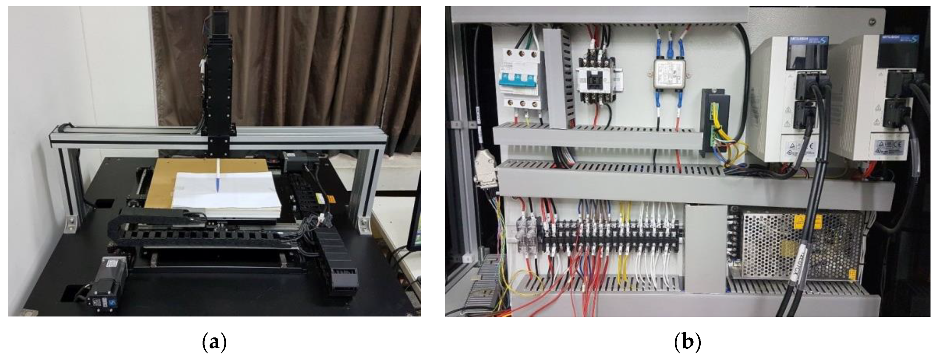
With $\mathrm{g}=1/\mathrm{m}$, $\mathrm{D}=\mathrm{g}\left({\mathrm{f}}_{\mathrm{b}}+{\mathrm{f}}_{\mathrm{u}}\right)$ where $\mathrm{D}$ is the lumped disturbance parameter bounded by ${\mathrm{D}}^{\mathrm{U}}$. It is assumed that $\left|\mathrm{D}\right|<{\mathrm{D}}^{\mathrm{U}}$. The experimental system of the proposed XY motion stage is depicted in Figure 1a,b.

2.2. Two-Dimensional FCMAC Architecture

A basic CMAC architecture [9] is shown in Figure 2. The mapping relation is described as:

$$\mathrm{Y} :\mathrm{y}\left(s\right)=AW,$$

(5)

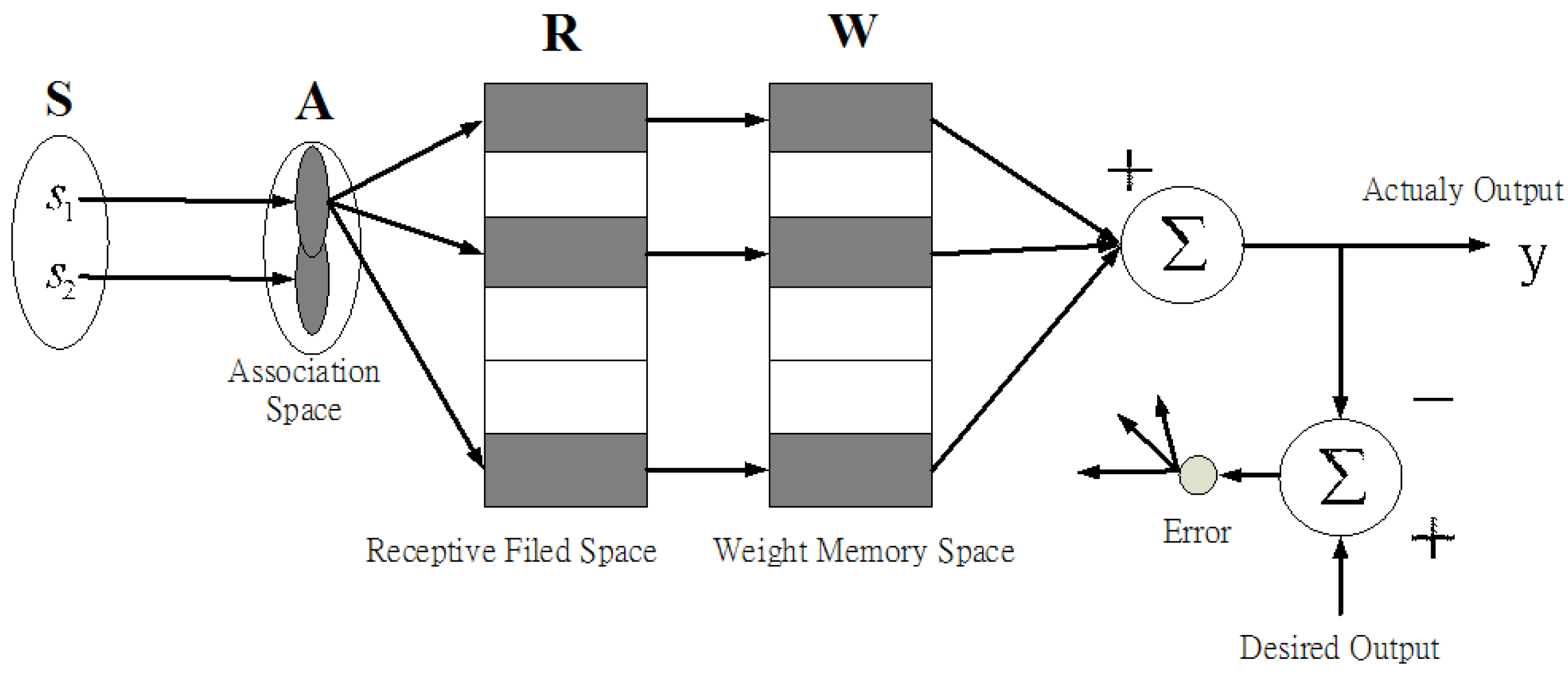
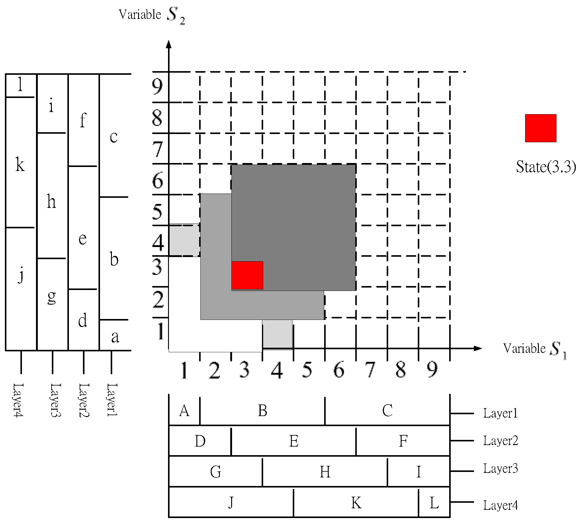
where $s$ is the continuous n-dimensional input space, $A$ is the association memory with ${\mathrm{n}}_{\mathrm{a}}$ elements, $R$ is the receptive field with ${\mathrm{n}}_{\mathrm{h}}$ elements, $W$ is the weight memory with ${\mathrm{n}}_{\mathrm{h}}$ adjustable weights, and $\mathrm{Y}$ is the m-dimensional output space. The mapping structure of the two-dimensional CMAC is depicted in Figure 3. In this case, two input variables, ${\mathrm{s}}_1$ and ${\mathrm{s}}_2$, are both quantized into nine intervals and divided into three blocks. Namely, ${\mathrm{s}}_1$ is divided into three blocks named A, B, C, and ${\mathrm{s}}_2$ is divided into a, b, c in the first layer. Then, ${\mathrm{s}}_1$ is shifted an interval to D, E, F, and so is ${\mathrm{s}}_2$ that shifted to d, e, f in the second layer, and so on. Therefore, Aa, Ab, Ac, Ba, Bb, Bc, Ca, Cb, Cc, which are called hypercubes, are obtained in the first layer and the same as Dd, De, Df, Ed, Ee, Ef, Fd, Fe, Ff that are in the second layer. Each hypercube is composed of the blocks in the same layer of two input variables; that is to say, it is impossible to obtain a hypercube, such as Ad, Ei, or Gc. In the case, there are 81 states, 36 hypercubes, and four layers, and each state activates four association cells that exists in different hypercubes. It means that $\mathrm{k}=81$, $\mathrm{m}=4$, and $\mathrm{n}=36$. The actual output of each state can be expressed as:

$${\mathrm{y}}_{\mathrm{sk}}=a_{\mathrm{sk}}^{\mathrm{T}}W=\left[\begin{array}{cccc}{a}_{\mathrm{sk},1}& a_{\mathrm{sk},2}& \dots & a_{\mathrm{sk},\mathrm{n}}\end{array}\right]\left[\begin{array}{c}{\mathrm{w}}_1\\ {\mathrm{w}}_2\\ ⋮\\ {\mathrm{w}}_n\end{array}\right]={\displaystyle \sum }_{\mathrm{j}=1}^{\mathrm{n}}{a}_{\mathrm{sk},\mathrm{j}}{\mathrm{w}}_{\mathrm{j}}$$

(6)

where $a_{\mathrm{sk}}^{\mathrm{T}}$ is the association index vector of the $\mathrm{k}\text{-}\mathrm{th}$ state and $W$ is the weight vector that comprises weights stored in memory. The collection of Equation (6) can be represented as:

$$\mathrm{Y}=\left[\begin{array}{c}{y}_{\mathrm{s}1}\\ y_{\mathrm{s}2}\\ ⋮\\ y_{\mathrm{sk}}\end{array}\right]=\left[\begin{array}{cccc}{a}_{\mathrm{s}1,1}& a_{\mathrm{s}1,2}& \dots & a_{\mathrm{s}1,\mathrm{n}}\\ a_{\mathrm{s}2,1}& a_{\mathrm{s}2,2}& \dots & a_{\mathrm{s}2,\mathrm{n}}\\ ⋮& & & \\ a_{\mathrm{sk},1}& a_{\mathrm{sk},2}& & a_{\mathrm{sk},\mathrm{n}}\end{array}\right]\left[\begin{array}{c}{\mathrm{w}}_1\\ {\mathrm{w}}_2\\ ⋮\\ {\mathrm{w}}_n\end{array}\right]=\left[\begin{array}{c}{a}_{\mathrm{sk}}^{\mathrm{T}}\\ a_{\mathrm{sk}}^{\mathrm{T}}\\ ⋮\\ a_{\mathrm{sk}}^{\mathrm{T}}\end{array}\right]\left[\begin{array}{c}{\mathrm{w}}_1\\ {\mathrm{w}}_2\\ ⋮\\ {\mathrm{w}}_n\end{array}\right]=\mathrm{AW}$$

(7)

and the matrix $A$ is expressed as:

$$A=\left[\begin{array}{c}{a}_{\mathrm{s}1}^{\mathrm{T}}\\ a_{\mathrm{s}2}^{\mathrm{T}}\\ ⋮\\ a_{81}^{\mathrm{T}}\end{array}\right]={\left[\begin{array}{ccccccccccccc}1& 0& 0& \cdots & 0& 1& 0& \cdots & 0& 1& 0& \cdots & 0\\ 0& 1& 0& \cdots & 0& 1& 0& \cdots & 0& 1& 0& \cdots & 0\\ ⋮& & & & & & & & & & & & \\ 0& 0& 0& \cdots & 1& 0& 0& \cdots & 1& 0& 0& \cdots & 1\end{array}\right]}_{81\times 36}$$

(8)

with

$$a_{\mathrm{s}21}^{\mathrm{T}}=\left[\begin{array}{cccccccccccccccccccc}0& 0& 0& 0& 1& 0& \cdots & 0& 1& 0& \cdots & 0& 1& 0& \cdots & 0& 1& 0& \cdots & 0\end{array}\right]$$

where it means that state (3,3) activates the hypercubes 5(Bb), 14(Ee), 19(Gg), and 28(Jj). The related weights are adjusted by the update law as

$$W\left(\mathrm{i}\right)=W\left(\mathrm{i}-1\right)+\Delta W=W\left(\mathrm{i}-1\right)+\frac{\mathsf{\alpha }}{\mathrm{m}}{a}_{\mathrm{sk}}\left({\mathrm{y}}_{\mathrm{sk}}^{\mathrm{d}}-a_{\mathrm{sk}}W\left(\mathrm{i}-1\right)\right)$$

(9)

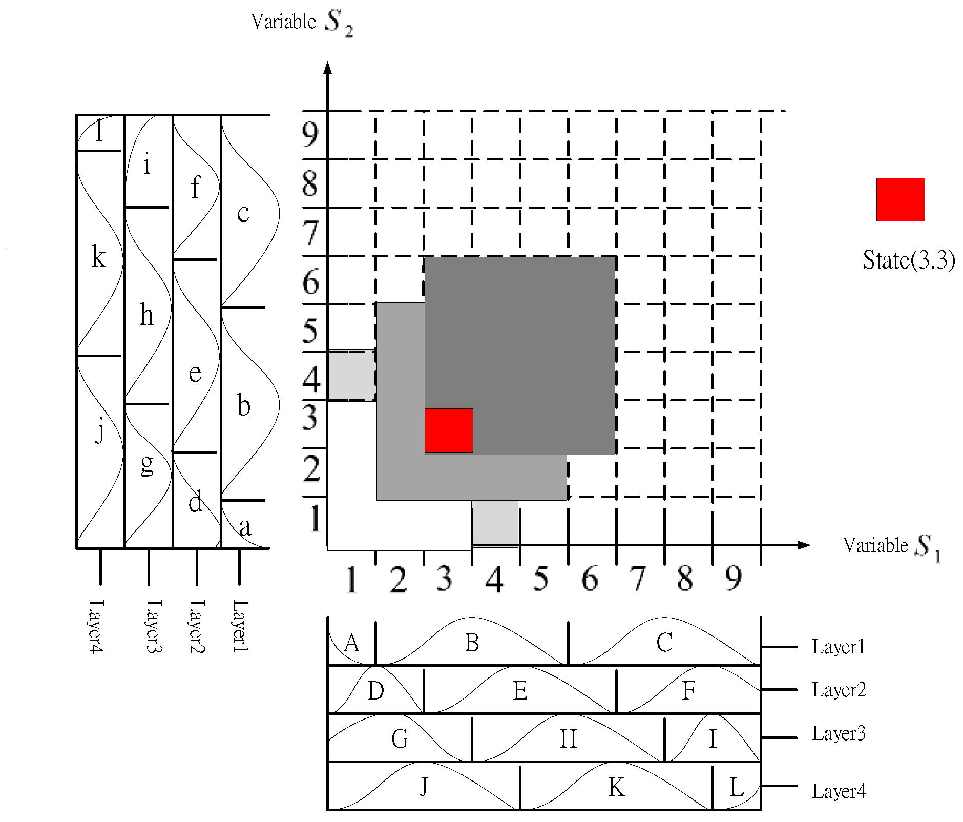
where $\mathrm{i}$ means the $\mathrm{i}\text{-}\mathrm{th}$ learning step, ${\mathrm{y}}_{\mathrm{sk}}^{\mathrm{d}}$ is the desired output, and $\mathsf{\alpha }$ is the learning rate. Through the above training process, FCMAC [9,10,11,12] is able to approximate the desired trajectory. The mapping structure of the two-dimensional CMAC with the Gaussian basis function is shown in Figure 4. Here, the Gaussian function is adopted as the receptive field basis function, and it is given as:

$${\mathsf{\phi }}_{\mathrm{ij}}\left({\mathrm{s}}_{\mathrm{i}}\right)=\exp \left[\frac{-{\left({\mathrm{s}}_{\mathrm{i}}-{\mathrm{m}}_{\mathrm{ij}}\right)}^2}{{\mathsf{\sigma }}_{\mathrm{ij}}^2}\right] \mathrm{for} \mathrm{j}=1,2\dots \dots ,12$$

(10)

where ${\mathsf{\phi }}_{\mathrm{ij}}\left({\mathrm{s}}_{\mathrm{i}}\right)$ presents the j-th block of the i-th input ${\mathrm{s}}_{\mathrm{i}}$ with the mean ${\mathrm{m}}_{\mathrm{ij}}$ and the variance ${\mathsf{\sigma }}_{\mathrm{ij}}$. Areas formed by blocks, named as Aa, Bb, and Cc, are called receptive fields. Each location of A is parallel to a receptive field. The two-dimensional receptive field function is defined as:

$${\mathrm{b}}_{\mathrm{k}}={\displaystyle \prod }_{\mathrm{i}=1}^2{\mathsf{\phi }}_{\mathrm{ij}}\left({\mathrm{s}}_{\mathrm{i}}\right) \mathrm{for} \mathrm{k}=1,2\dots \dots ,\mathrm{n}$$

(11)

where ${\mathrm{b}}_{\mathrm{k}}$ is associated with the k-th receptive field. As for the results, the output of CMAC with the Gaussian basis function can be expressed as

$$\mathrm{y}=a_{\mathrm{sk}}^{\mathrm{T}}\left[\begin{array}{cccc}{\mathrm{b}}_1& 0& \cdots & 0\\ 0& {\mathrm{b}}_2& \cdots & 0\\ ⋮& & \ddots & \\ 0& 0& \cdots & {\mathrm{b}}_{\mathrm{n}}\end{array}\right]w={\xi }^{\mathrm{T}}w=w^{\mathrm{T}}\xi$$

(12)

with ${\xi }^{\mathrm{T}}\triangleq a_{\mathrm{sk}}^{\mathrm{T}}\left[\begin{array}{cccc}{\mathrm{b}}_1& 0& \cdots & 0\\ 0& {\mathrm{b}}_2& \cdots & 0\\ ⋮& & \ddots & \\ 0& 0& \cdots & {\mathrm{b}}_{\mathrm{n}}\end{array}\right]$.

The mechanical system of a motion stage system with system uncertainty can be generally rewritten as a second-order nonlinear system. It is given by [4]

$$\ddot{\mathrm{x}}=\mathrm{f}\left(x\right)+\mathrm{b}\left(x\right)\mathrm{u}+\mathrm{d}\left(\mathrm{t}\right)$$

(13)

$$\mathrm{y}=\mathrm{x},$$

(14)

where $\mathrm{x}$ is the stage X- or Y-axis displacement, and $X={\left[\begin{array}{cc}{\mathrm{x}}_1& {\mathrm{x}}_2\end{array}\right]}^{\mathrm{T}}=\left[\begin{array}{cc}\mathrm{x}& \dot{\mathrm{x}}\end{array}\right]\in {\mathrm{R}}^2$ is the state vector of the system. $\mathrm{f}\left(x\right)$ and $\mathrm{b}\left(x\right)$ are the bounded real continuous nonlinear functions, $\mathrm{u}\in \mathrm{R}$ is the control input, $\mathrm{y}\in \mathrm{R}$ is the system output, and $\mathrm{d}$ is the bounded disturbance that cannot be measured. It is assumed that the system in Equations (13) and (14) is controllable, and it is required that $\mathrm{b}\left(x\right)\ne 0$ for vector $X$ in certain controllability regions. It is assumed that $0<\mathrm{b}\left(x\right)<\infty$.

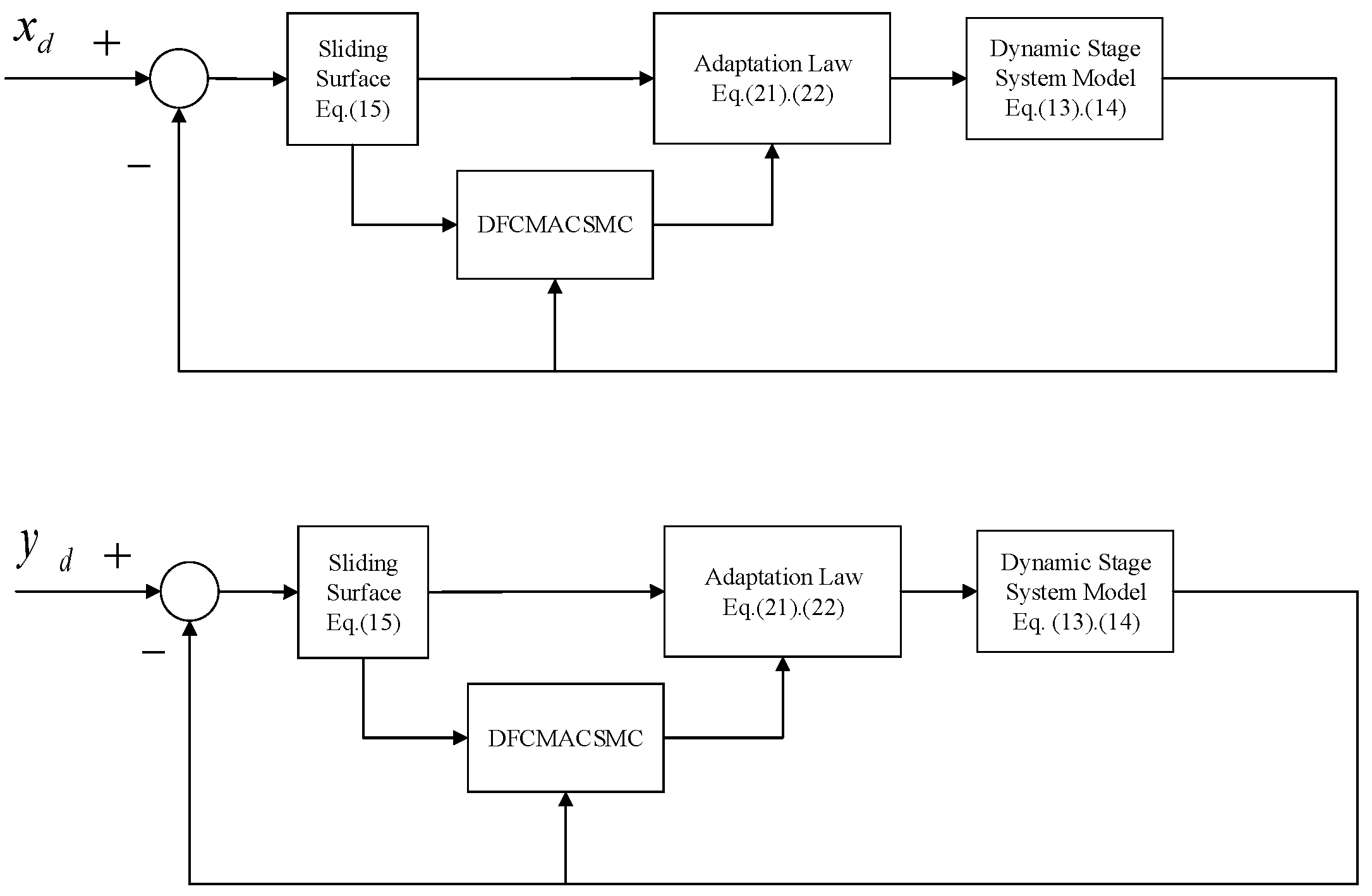
Figure 5 demonstrates the architecture of the proposed DFCMACSMC method for the two-axis motion system. The output tracking error is defined as $\mathrm{e}={\mathrm{x}}_{\mathrm{d}}-\mathrm{y}={\mathrm{x}}_{\mathrm{d}}-\mathrm{x}$, and the tracking error vector is $\mathrm{E}={\left[\begin{array}{cc}\mathrm{e}& \dot{\mathrm{e}}\end{array}\right]}^{\mathrm{T}}={\left[\begin{array}{cc}{\mathrm{e}}_1& {\mathrm{e}}_2\end{array}\right]}^{\mathrm{T}}$.

The sliding surface parameter $\mathrm{s}$ is defined as follows:

$$\mathrm{s}=-\left(cE\right)=-\left({\mathrm{c}}_1\mathrm{e}+\dot{\mathrm{e}}\right)$$

(15)

with $c=\left[\begin{array}{cc}{\mathrm{c}}_1& 1\end{array}\right].$

To guarantee that the trajectory of the state error vector $e$ will transfer from the approaching phase to the sliding phase, the sufficient condition is

$$\mathrm{s}\dot{\mathrm{s}}=-\mathsf{\eta }\left|\mathrm{s}\right| , \mathsf{\eta }>0.$$

(16)

Since $\mathrm{f}\left(x\right)$ and $\mathrm{b}\left(x\right)$ are known and free of external disturbances, the derivative of the sliding surface is taken with respect to time as a zero-value. It becomes

$$\dot{\mathrm{s}}=-\left({\mathrm{c}}_1\dot{\mathrm{e}}+\ddot{\mathrm{e}}\right)=-\left({\mathrm{c}}_1\dot{\mathrm{e}}+{\ddot{\mathrm{x}}}_{\mathrm{d}}-\ddot{\mathrm{x}}\right)=-\left({\mathrm{c}}_1\dot{\mathrm{e}}-\mathrm{f}\left(x\right)-\mathrm{b}\left(x\right){\mathrm{u}}_{\mathrm{eq}}\right)-{\ddot{\mathrm{x}}}_{\mathrm{d}}=0.$$

(17)

Therefore, the equivalent control can be obtained as follows:

$${\mathrm{u}}_{\mathrm{eq}}=\frac{1}{\mathrm{b}\left(x\right)}\left({\mathrm{c}}_1\dot{\mathrm{e}}-\mathrm{f}\left(x\right)+{\ddot{\mathrm{x}}}_{\mathrm{d}}\right)$$

(18)

In the approaching phase, $\mathrm{s}\ne 0$, an approaching-type control ${\mathrm{u}}_{\mathrm{ap}}$ must be added to satisfy the sufficient condition and complete sliding mode control. It can be expressed as:

$$\mathrm{u}={\mathrm{u}}_{\mathrm{eq}}=\frac{{\mathrm{u}}_{\mathrm{ap}}}{\mathrm{b}\left(x\right)}$$

(19)

with

$${\mathrm{u}}_{\mathrm{ap}}={\mathsf{\eta }}_{∆}\mathrm{sgn}\left(\mathrm{s}\right) ,{ \mathsf{\eta }}_{∆}=\mathrm{D}+\mathsf{\eta }\hspace{1em}{\mathsf{\eta }}_{∆}\ge \mathsf{\eta }\ge 0 \mathrm{sgn}\left(\mathrm{s}\right)=\{\begin{array}{c}1\\ 0\\ -1\end{array} \begin{array}{c}\mathrm{s}>0\\ \mathrm{s}=0\\ \mathrm{s}<0\end{array}$$

where ${\mathrm{u}}_{\mathrm{eq}}$ is the equivalent control input, and ${\mathsf{\eta }}_{∆}$ and $\mathsf{\eta }$ are positive constants.

Replacing ${\mathrm{u}}_{\mathrm{eq}}$ in Equation (18) by the FCMAC $\mathrm{u}\left(x|\mathsf{\theta }\right)$ gives

$$\mathrm{u}\left(x|\mathsf{\theta }\right)={\xi }^{\mathrm{T}}\mathsf{\theta }.$$

(20)

The control input $\mathrm{u}$ and the adaptive laws are chosen as:

$$\mathrm{u}={\mathrm{u}}_{\mathrm{D}}\left(x|\mathsf{\theta }\right)-\frac{\mathsf{\eta } \mathrm{sgn}\left(\mathrm{s}\right)}{\mathrm{b}\left(x\right)}$$

(21)

$$\dot{\mathsf{\theta }}=-2{\mathrm{r}}_1\mathrm{sb}\left(x\right)\mathsf{\xi }\left(x\right).$$

(22)

The optimal parameters ${\mathsf{\theta }}^{*}$ is defined as follows:

$${\mathsf{\theta }}^{*}=\arg \underset{\mathsf{\theta }={\mathsf{\Omega }}_{\mathsf{\theta }}}{\min }\left[\underset{\mathrm{x}\in {\mathsf{\Omega }}_{\mathrm{x}}}{\sup }\left|{\mathrm{u}}_{\mathrm{D}}\left(x|\mathsf{\theta }\right)-{\mathrm{u}}_{\mathrm{eq}}\right|\right],$$

(23)

where ${\mathsf{\Omega }}_{\mathsf{\theta }}$ and ${\mathsf{\Omega }}_{\mathrm{x}}$ are the set of suitable bounds on $\mathsf{\theta }$ and $x$, respectively.

The minimum approximation error is defined as:

$$\mathsf{\omega }=\mathrm{b}\left(x\right)\left({\mathrm{u}}_{\mathrm{D}}\left(x|{\mathsf{\theta }}^{*}\right)-{\mathrm{u}}_{\mathrm{eq}}\right)+\mathrm{d}\left(\mathrm{t}\right).$$

(24)

The time derivative of the sliding surface is

$$\begin{array}{c}\dot{\mathrm{s}}=-\left({\mathrm{c}}_1\dot{\mathrm{e}}+{\ddot{\mathrm{x}}}_{\mathrm{d}}-\ddot{\mathrm{x}}\right)\\ =-\left({\mathrm{c}}_1\dot{\mathrm{e}}-\mathrm{f}\left(x\right)-\mathrm{b}\left(x\right)\mathrm{u}-\mathrm{d}\left(\mathrm{t}\right)\right)-{\ddot{\mathrm{x}}}_{\mathrm{d}}\\ =-{\mathrm{c}}_1\dot{\mathrm{e}}+\mathrm{f}\left(x\right)+\mathrm{b}\left(x\right)\mathrm{u}+\mathrm{d}\left(\mathrm{t}\right)-{\ddot{\mathrm{x}}}_{\mathrm{d}}\\ =-{\mathrm{c}}_1\dot{\mathrm{e}}+\mathrm{f}\left(x\right)+\mathrm{b}\left(x\right)\mathrm{u}+\mathrm{d}\left(\mathrm{t}\right)-{\ddot{\mathrm{x}}}_{\mathrm{d}}+\mathsf{\omega }-\mathrm{b}\left(x\right)\left({\mathrm{u}}_{\mathrm{D}}\left(x|{\mathsf{\theta }}^{*}\right)-{\mathrm{u}}_{\mathrm{eq}}\right)-\mathrm{d}\left(\mathrm{t}\right)\\ =\mathrm{b}\left(x\right)\left({\mathrm{u}}_{\mathrm{D}}\left(x|\mathsf{\theta }\right)-\frac{\mathsf{\eta } \mathrm{sgn}\left(\mathrm{s}\right)}{\mathrm{b}\left(x\right)}\right)+\mathsf{\omega }-\mathrm{b}\left(x\right)\left({\mathrm{u}}_{\mathrm{D}}\left(x|{\mathsf{\theta }}^{*}\right)\right)\\ =-\mathsf{\eta }\mathrm{sgn}\left(\mathrm{s}\right)+\mathsf{\omega }+\mathrm{b}\left(x\right)\left({\mathrm{u}}_{\mathrm{D}}\left(x|\mathsf{\theta }\right)\right)-\mathrm{b}\left(x\right)\left({\mathrm{u}}_{\mathrm{D}}\left(x|{\mathsf{\theta }}^{*}\right)\right)\\ =-\mathsf{\eta }\mathrm{sgn}\left(\mathrm{s}\right)+\mathsf{\omega }+\mathrm{b}\left(x\right)\left({\mathrm{u}}_{\mathrm{D}}\left(x|\mathsf{\theta }\right)-{\mathrm{u}}_{\mathrm{D}}\left(x|{\mathsf{\theta }}^{*}\right)\right)=-\mathsf{\eta }\mathrm{sgn}\left(\mathrm{s}\right)+\mathsf{\omega }+\mathrm{b}\left(x\right){\tilde{\mathsf{\theta }}}^{\mathrm{T}}\mathsf{\xi }\left(x\right)\end{array}$$

(25)

The Lyapunov function is defined as:

$${\mathrm{V}}_{\mathrm{DFCMACSMC}}=({\mathrm{s}}^2+\frac{1}{2{\mathrm{r}}_1}{\tilde{\mathsf{\theta }}}^{\mathrm{T}}\tilde{\mathsf{\theta }})$$

(26)

with $\tilde{\mathsf{\theta }}=\mathsf{\theta }-{\mathsf{\theta }}^{*}$.

The time derivative of function $\mathrm{V}$ can be expressed as follows:

$$\begin{array}{c}{\dot{\mathrm{V}}}_{\mathrm{DFCMACSMC}}=\mathrm{s}\dot{\mathrm{s}}+\frac{1}{2{\mathrm{r}}_1}{\dot{\tilde{\mathsf{\theta }}}}^{\mathrm{T}}\tilde{\mathsf{\theta }}+\frac{1}{2{\mathrm{r}}_1}{\tilde{\mathsf{\theta }}}^{\mathrm{T}}\dot{\tilde{\mathsf{\theta }}}\\ =\mathrm{s}\left(-\mathsf{\eta }\mathrm{sgn}\left(\mathrm{s}\right)+\mathsf{\omega }+\mathrm{b}\left(x\right){\tilde{\mathsf{\theta }}}^{\mathrm{T}}\xi \left(x\right)\right)+\frac{1}{{\mathrm{r}}_1}{\tilde{\mathsf{\theta }}}^{\mathrm{T}}\dot{\tilde{\mathsf{\theta }}} \\ =\mathrm{sb}\left(x\right){\tilde{\mathsf{\theta }}}^{\mathrm{T}}\xi \left(x\right)+\frac{1}{{\mathrm{r}}_1}{\tilde{\mathsf{\theta }}}^{\mathrm{T}}\dot{\tilde{\mathsf{\theta }}}-\mathrm{s}\mathsf{\eta }\mathrm{sgn}\left(\mathrm{s}\right)+\mathrm{s}\mathsf{\omega }\\ =\frac{1}{{\mathrm{r}}_1}{\tilde{\mathsf{\theta }}}^{\mathrm{T}}\left(\dot{\tilde{\mathsf{\theta }}}+{\mathrm{r}}_1\mathrm{sb}\left(x\right)\xi \left(x\right)\right)-\mathrm{s}\mathsf{\eta }\mathrm{sgn}\left(\mathrm{s}\right)+\mathrm{s}\mathsf{\omega }=-\mathrm{s}\mathsf{\eta }\mathrm{sgn}\left(\mathrm{s}\right)+\mathrm{s}\mathsf{\omega }\le 0\end{array}$$

(27)

with $\dot{\tilde{\mathsf{\theta }}}=\dot{\mathsf{\theta }}$.

By choosing ${\mathsf{\eta }}_{\mathrm{d}}>0$, Equation (31) is given as follows:

$${\dot{\mathrm{V}}}_{\mathrm{DFCMACSMC}}\le -\left|\mathsf{\omega }\right|\left|\mathrm{s}\right|-\mathsf{\eta }\left|\mathrm{s}\right|\le -{\mathsf{\eta }}_{\mathrm{d}}\left|\mathrm{s}\right|$$

(28)

with ${\mathsf{\eta }}_{\mathrm{d}}=\left(\mathsf{\eta }+\left|\mathsf{\omega }\right|\right)$.

Integrating the above equation, it yields

$$\underset{0}{\overset{\mathrm{t}}{{\displaystyle \int }}}|\mathrm{s}(\mathsf{\tau })|\mathrm{d}\mathsf{\tau }\le \frac{1}{{\mathsf{\eta }}_{\mathrm{d}}}\left[{\mathrm{V}}_{\mathrm{DFCMACSMC}}\left(0\right)-{\mathrm{V}}_{\mathrm{DFCMACSMC}}\left(\mathrm{t}\right)\right]$$

(29)

Since ${\mathrm{V}}_{\mathrm{DFCMACSMC}}(0)$ is bounded, and ${\mathrm{V}}_{\mathrm{DFCMACSMC}}(\mathrm{t})$ is nonincreasing and bounded, the following equation can be conducted:

$$\underset{0}{\overset{\mathrm{t}}{{\displaystyle \int }}}|\mathrm{s}(\mathsf{\tau })|\mathrm{d}\mathsf{\tau }\le \infty$$

(30)

Furthermore, $\dot{\mathrm{s}}\left(\mathsf{\tau }\right)$ is also bounded. The $\mathrm{s}\left(\mathsf{\tau }\right)$ is uniformly continuous. Using Barbalat’s lemma [16], the following result can be obtained:

$$\underset{\mathrm{t}\to \infty }{\lim }\mathrm{s}\left(\mathrm{t}\right)=0$$

(31)

It can be implied that ${\lim }_{\mathrm{t}\to \infty }\left|\mathrm{e}\left(\mathrm{t}\right)\right|=0$. The DFCMACSMC system is stable, and the error will converge to zero asymptotically [19,20,21,22]. The proposed system guarantees the asymptotical stability of the tracking error $\mathrm{e}\left(\mathrm{t}\right)$, even with the parameter variations and external disturbances.

3. Results

3.1. Contour Planning

The NURBS [23] curve is applied to optimize the trajectory point to obtain the smooth trajectory. The NURBS curve expression is defined as follows:

$$\mathrm{F}\left(\mathrm{u}\right)=\frac{{{\displaystyle \sum }}_{i=0}^n{w}_i{D}_i{N}_{i,k}\left(u\right)}{{{\displaystyle \sum }}_{i=0}^n{w}_i{N}_{i,k}\left(u\right)}$$

(32)

$$N_{i,0}=\{\begin{array}{cc}1& u_i\le u_{}\le u_{i+1}\\ 0& otherwise\end{array}$$

(33)

$$N_{i,m}=\frac{\left(u_{}-u_i\right)N_{i,m-1}\left(u\right)}{u_{i+m}-u_i}+\frac{\left(u_{i+m+1}-u_{}\right)N_{i+1,m-1}\left(u\right)}{u_{i+m+1}-u_{i+1}}, m\ge 1$$

(34)

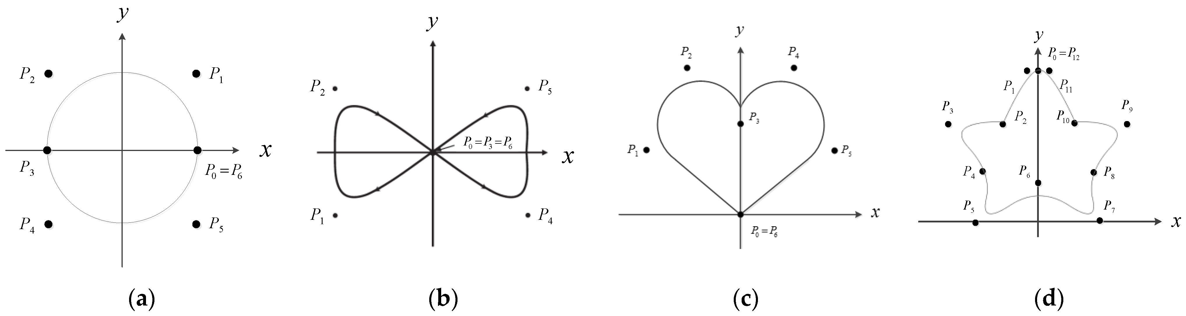
with $\mathrm{U}=\left[u_o,u_1,\cdots ,u_{n+k+1}\right],$ where $u$ is the control variable of the curve, $\mathrm{k}$ is the power exponent of the interpolation basis function, $\mathrm{n}$ is the number of interpolation points, and $w_i$ is the weight factor, whose number is the same as the control variable. $N_{i,k}$ is the basis function, which is selected according to the node vector. Four contour shapes were applied for this proposed adaptive DFCMAC control system, namely, the circular, bowknot, heart, and star curves.

Table 1. The four types of trajectory planning.

Trajectory Type	Segment Functions
Circle contour	$\begin{array}{c}{\mathrm{k}}_{\mathrm{d}}=2\\ V=[{\mathrm{V}}_0,{\mathrm{V}}_1,{\mathrm{V}}_2,{\mathrm{V}}_3,{\mathrm{V}}_4,{\mathrm{V}}_5,{\mathrm{V}}_6]=[(2.5,0),(2.5,2.5),(-2.5,2.5),(-2.5,0),(-2.5,-2.5),(2.5,-2.5),(2.5,0)]\end{array}$ (unit: cm, cm) $\begin{array}{c}\mathbf{P}=[{\mathrm{P}}_0,{\mathrm{P}}_1,{\mathrm{P}}_2,{\mathrm{P}}_3,{\mathrm{P}}_4,{\mathrm{P}}_5,{\mathrm{P}}_6,{\mathrm{P}}_7,{\mathrm{P}}_8,{\mathrm{P}}_9]=[0,0,0,0.25,0.5,0.5,0.75,1,1,1]\\ \mathbf{w}=\left[{\mathrm{w}}_0,{\mathrm{w}}_1,{\mathrm{w}}_2,{\mathrm{w}}_3,{\mathrm{w}}_4,{\mathrm{w}}_5,{\mathrm{w}}_6\right]=[1,0.5,0.5,1,0.5,0.5,1]\end{array}$
Bowknot contour	$\begin{array}{c}{\mathrm{k}}_{\mathrm{d}}=2\\ V=[{\mathrm{V}}_0,{\mathrm{V}}_1,{\mathrm{V}}_2,{\mathrm{V}}_3,{\mathrm{V}}_4,{\mathrm{V}}_5,{\mathrm{V}}_6]=[(0,0),(-1.5,-1.5),(-1.5,1.5),(0,0),(1.5,-1.5),(1.5,1.5),(0,0)]\end{array}$ (unit: cm, cm) $\mathbf{P}=[{\mathrm{P}}_0,{\mathrm{P}}_1,{\mathrm{P}}_2,{\mathrm{P}}_3,{\mathrm{P}}_4,{\mathrm{P}}_5,{\mathrm{P}}_6,{\mathrm{P}}_7,{\mathrm{P}}_8,{\mathrm{P}}_9]=[0,0,0,0.25,0.5,0.5,0.75,1,1,1]$ $\mathbf{w}=\left[{\mathrm{w}}_0,{\mathrm{w}}_1,{\mathrm{w}}_2,{\mathrm{w}}_3,{\mathrm{w}}_4,{\mathrm{w}}_5,{\mathrm{w}}_6\right]=[1,2.5,2.5,1,2.5,2.5,1]$
Heart contour	$\begin{array}{l}{\mathrm{k}}_{\mathrm{d}}=2\\ V=[{\mathrm{V}}_0,{\mathrm{V}}_1,{\mathrm{V}}_2,{\mathrm{V}}_3,{\mathrm{V}}_4,{\mathrm{V}}_5,{\mathrm{V}}_6]=[(0,0),(-3,2),(-2,5),(0,3.6),(2,5),(3,1),(0,0)]\end{array}$(unit: cm, cm) $P=[{\mathrm{P}}_0,{\mathrm{P}}_1,{\mathrm{P}}_2,{\mathrm{P}}_3,{\mathrm{P}}_4,{\mathrm{P}}_5,{\mathrm{P}}_6,{\mathrm{P}}_7,{\mathrm{P}}_8,{\mathrm{P}}_9]=[0,0,0,0.25,0.5,0.5,0.75,1,1,1]$ $w=\left[{\mathrm{w}}_0,{\mathrm{w}}_1,{\mathrm{w}}_2,{\mathrm{w}}_3,{\mathrm{w}}_4,{\mathrm{w}}_5,{\mathrm{w}}_6\right]=[1,1,1,1,1,1,1]$
Star contour	$\begin{array}{c}{\mathrm{k}}_{\mathrm{d}}=2\\ V=[{\mathrm{V}}_0,{\mathrm{V}}_1,{\mathrm{V}}_2,{\mathrm{V}}_3,{\mathrm{V}}_4,{\mathrm{V}}_5,{\mathrm{V}}_6,{\mathrm{V}}_7,{\mathrm{V}}_8,{\mathrm{V}}_9,{\mathrm{V}}_{10},{\mathrm{V}}_{11},{\mathrm{V}}_{12}]\\ =[(0,6),(-0.5,6),(-1.5,4),(-4,4),(-2,2),(-2.5,0),(0,1.5)\\ ,(2.5,0),(2,2),(4,4)(1.5,4),(0.5,6),(0,6)]\end{array}$            (unit: cm, cm) $P=[{\mathrm{P}}_0,{\mathrm{P}}_1,{\mathrm{P}}_2,{\mathrm{P}}_3,{\mathrm{P}}_4,{\mathrm{P}}_5,{\mathrm{P}}_6,{\mathrm{P}}_7,{\mathrm{P}}_8,{\mathrm{P}}_9,{\mathrm{P}}_{10},{\mathrm{P}}_{11},{\mathrm{P}}_{12},{\mathrm{P}}_{13},{\mathrm{P}}_{14}]=[0,0,0,0.1,0.1,0.2,0.3,0.4,0.5,0.6,0.7,0.8,0.8,1,1,1]$ $w=\left[{\mathrm{w}}_0,{\mathrm{w}}_1,{\mathrm{w}}_2,{\mathrm{w}}_3,{\mathrm{w}}_4,{\mathrm{w}}_5,{\mathrm{w}}_6,{\mathrm{w}}_7,{\mathrm{w}}_8,{\mathrm{w}}_9,{\mathrm{w}}_{10},{\mathrm{w}}_{11},{\mathrm{w}}_{12}\right]=[1,1,1,1,1,1,1,1,1,1,1,1,1]$

lists the parameters of these four contours. Figure 6a–d depicts the desired contours based on the abovementioned parameter setting.

3.2. Parameter Setting and Performance Measurement

The average tracking error (ATE, ${\mathrm{T}}_{\mathrm{E}}$) and tracking error standard deviation (TESD,${ \mathrm{T}}_{\mathrm{S}}$) are selected as the performance indices, which is defined as follows:

$${\mathrm{T}}_{\mathrm{E}}={\displaystyle \sum }_{\mathrm{k}=1}^{\mathrm{K}}\frac{\mathrm{E}\left(\mathrm{k}\right)}{\mathrm{n}}$$

(35)

$${ \mathrm{T}}_{\mathrm{S}}=\sqrt{\frac{{{\displaystyle \sum }}_{\mathrm{k}=1}^{\mathrm{K}}{(\mathrm{E}\left(\mathrm{k}\right)-{\mathrm{T}}_{\mathrm{E}})}^2}{\mathrm{K}}}$$

(36)

with

$$\mathrm{E}\left(\mathrm{k}\right)=\sqrt{{\mathrm{e}}_{\mathrm{x}}^2\left(\mathrm{k}\right)+{\mathrm{e}}_{\mathrm{y}}^2\left(\mathrm{k}\right)},$$

where ${\mathrm{e}}_{\mathrm{x}}(\mathrm{k})$ is the tracking error in the x-axis, ${\mathrm{e}}_{\mathrm{y}}\left(\mathrm{k}\right)$ is the tracking error in the y-axis, and $\mathrm{K}$ is the total number of contour points. Two types of control algorithms are considered herein: (a) the direct adaptive conventional CMAC sliding method, and (b) the proposed adaptive DFCMAC sliding method.

In our experiments, the learning parameters are selected as: (a) The conventional CMAC method:${ \mathrm{r}}_{1\mathrm{x}}={\mathrm{r}}_{1\mathrm{y}}=0.001,{\mathrm{c}}_{1\mathrm{x}}={\mathrm{c}}_{1\mathrm{y}}=1,$ $\mathsf{\eta }=1$; and (b) the proposed DFCMACSMC method:${ \mathrm{r}}_{1\mathrm{x}}={\mathrm{r}}_{1\mathrm{y}}=0.001,{\mathrm{c}}_{1\mathrm{x}}={\mathrm{c}}_{1\mathrm{y}}=1,\mathrm{m}=0.5,\mathsf{\sigma }=1,$ $\mathsf{\eta }=1$. To verify the advancement of the DFCMACSMC method, four simulations are investigated.

The system parameters and Stribeck friction models of the X-Y stage are assumed as follows:

X-axis: ${\mathrm{K}}_{\mathrm{t}\mathrm{x}}=0.96 \mathrm{N}/\mathrm{A}$, ${\mathrm{M}}_{\mathrm{x}}=3\times {10}^{-3} \mathrm{N} {\mathrm{s}}^2/\mathrm{m}$, ${\mathrm{B}}_{\mathrm{x}}=0.1 \mathrm{N} \mathrm{s}/\mathrm{m}$, ${\mathrm{F}}_{\mathrm{L}\mathrm{x}}=0.1 \mathrm{N}$, ${\mathrm{F}}_{\mathrm{c}\mathrm{x}}=0.15 \mathrm{N}$, ${\mathrm{F}}_{\mathrm{s}\mathrm{x}}=0.24 \mathrm{N}$, ${\mathrm{V}}_{\mathrm{s}\mathrm{x}}=10 \mathrm{m}/\mathrm{s}$.

Y-axis: ${\mathrm{K}}_{\mathrm{t}\mathrm{y}}=0.96 \mathrm{N}/\mathrm{A}$, ${\mathrm{M}}_{\mathrm{y}}=2.8\times {10}^{-3} \mathrm{N} {\mathrm{s}}^2/\mathrm{m}$, ${\mathrm{B}}_{\mathrm{y}}=0.12 \mathrm{N}\mathrm{s}/\mathrm{m}$, ${\mathrm{F}}_{\mathrm{L}\mathrm{y}}=0.1 \mathrm{N}$, ${\mathrm{F}}_{\mathrm{c}\mathrm{y}}=0.15 \mathrm{N}$, ${\mathrm{F}}_{\mathrm{s}\mathrm{y}}=0.2 \mathrm{N}$, ${\mathrm{V}}_{\mathrm{s}\mathrm{y}}=5 \mathrm{m}/\mathrm{s}$.

3.3. Simulation

The results derived from the conventional CMAC methods and those results generated from our proposed method were compared and evaluated.

(a)

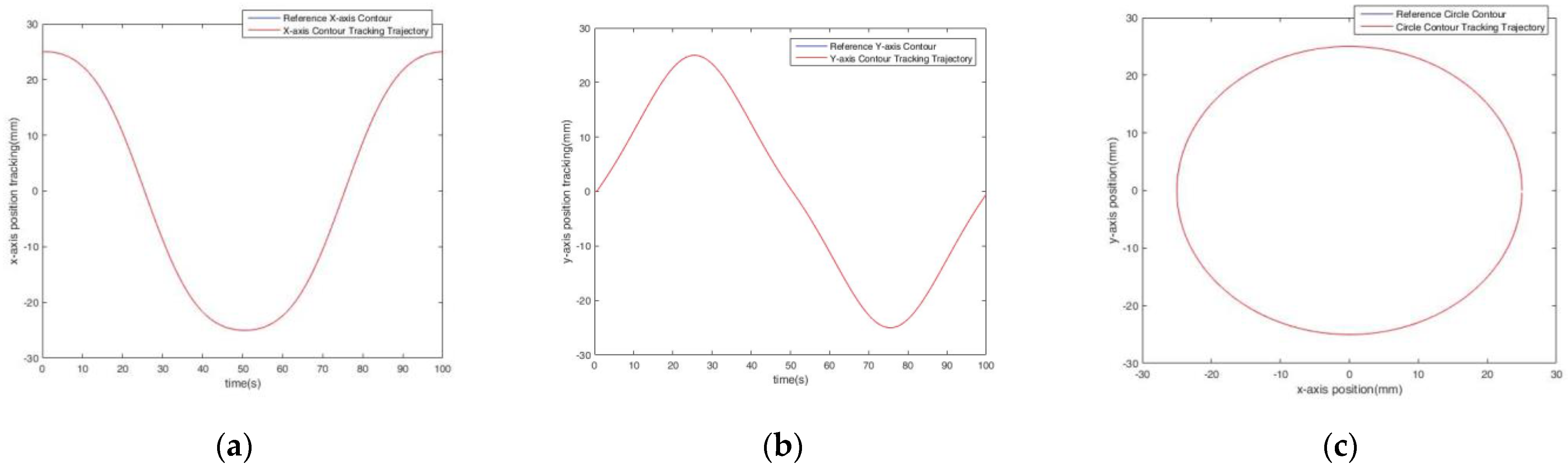
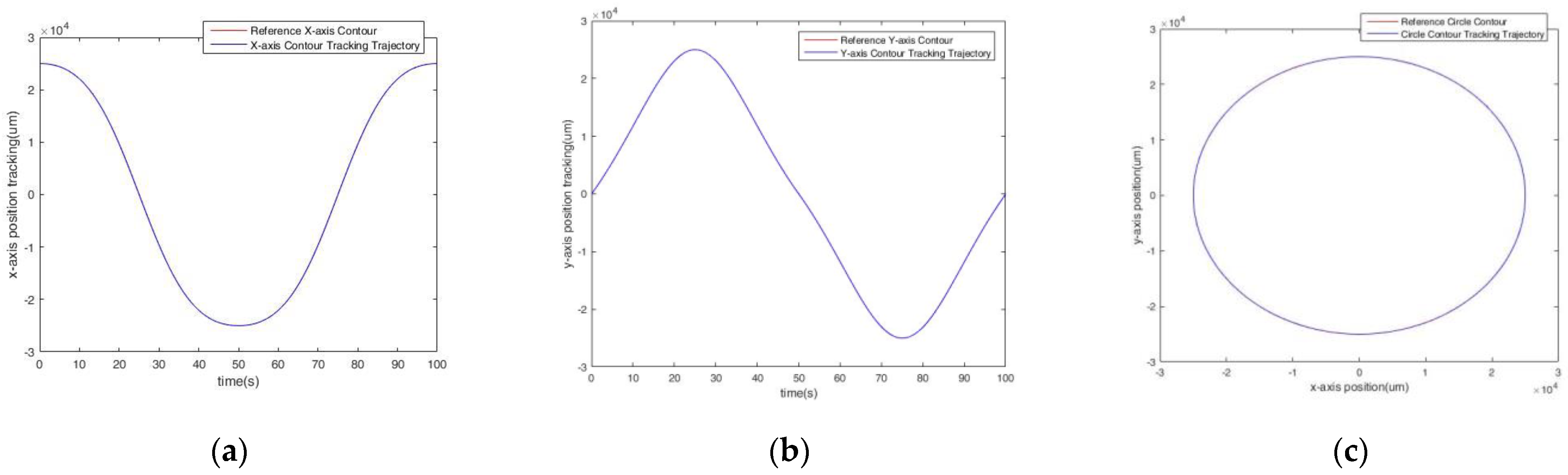
The circle contour was evaluated to show the tracking results observed in the X and Y axes, respectively. The simulation results are illustrated in Figure 7a–c. It shows that the proposed DFCMACSMC method performed well for trajectory tracking. The average of ATE index was 22.51 $\mathsf{\mu }\mathrm{m}$, and the average of TESD was 7.92 $\mathsf{\mu }\mathrm{m}$.

(b)

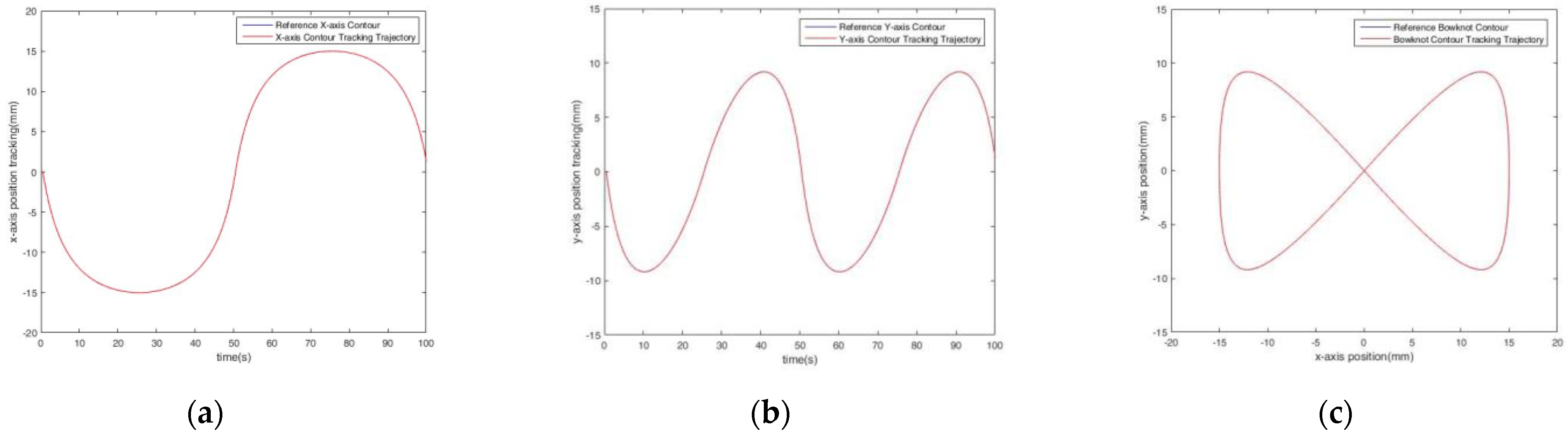
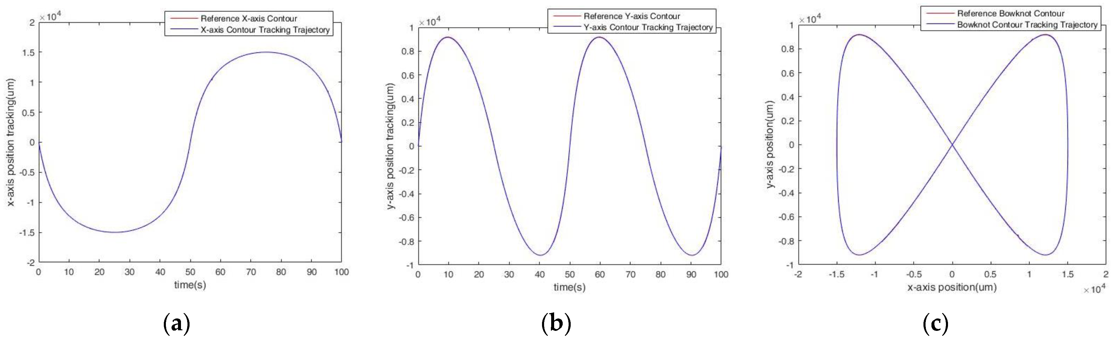
In the bowknot trajectory case, this method also behaves well in the X-axis and Y-axis displacement response, as shown in Figure 8a–c. The average of the ATE index was 21.79 μm, and the average of TESD was 7.62 μm in the bowknot case.

(c)

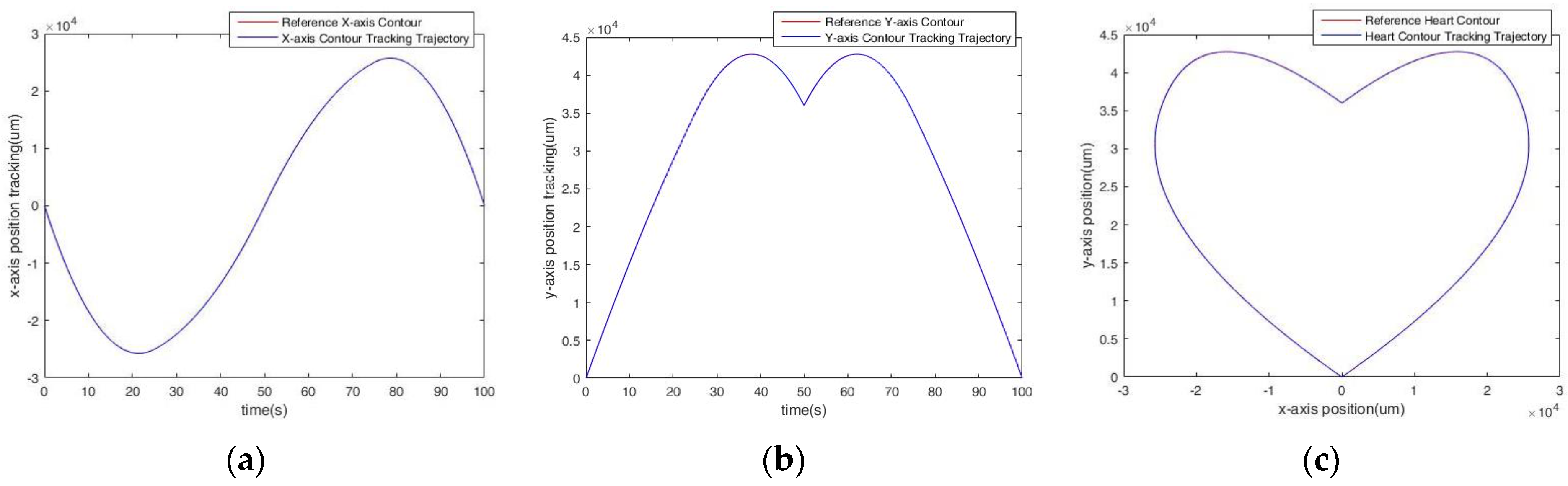
The third specific application was the heart trajectory. Figure 9a–c indicates that the position errors of the X and Y axes reduced significantly during the tracking process for the two-axis system. The average of the ATE index was 27.22 $\mathsf{\mu }\mathrm{m}$, and the average of TESD was 9.52 $\mathsf{\mu }\mathrm{m}$ in the heart case.

(d)

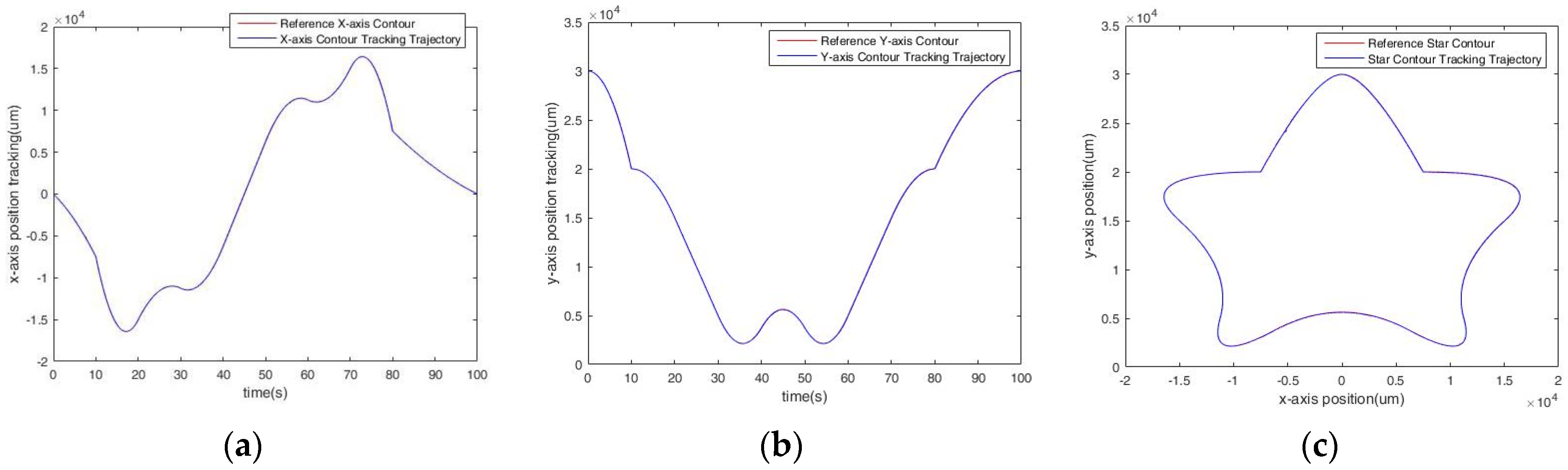
The star trajectory that we designed generated the total control point, defined as 13. Figure 10a–c shows the two-dimensional trajectories. The DFCMACSMC architecture could better achieve the tracking performance, and the trajectory error decreased at a steady state. The average of the ATE index was 21.88 $\mathsf{\mu }\mathrm{m}$, and the average of the TESD was 7.66 $\mathsf{\mu }\mathrm{m}$.

The proposed DFCMACSMC is compared to the conventional CMAC method shown in

Table 2. The simulated results showing contour tracking errors.

	$\mathbf{Average} \mathbf{Tracking} \mathbf{Error} \left(\mathbf{ATE}\right) E_M \left(\mathsf{\mu }\mathbf{m}\right)$
Trajectory Contour	The Conventional CMAC Method	The PROPOSED DFCMACSMC Method
Circle contour	50.04	22.51
Bowknot contour	32.89	21.79
Heart contour	48.67	27.22
Star contour	32.79	21.88
Average	41.09	23.35
	$\mathrm{Tracking} \mathrm{Error} \mathrm{Standard} \mathrm{Deviation} \left(\mathrm{TESD}\right) E_{\mathrm{STD}} \left(\mathsf{\mu }m\right)$
Trajectory Contour	The Conventional CMAC Method	The Proposed DFCMACSMC Method
Circle contour	17.53	7.92
Bowknot contour	11.48	7.62
Heart contour	17.04	9.52
Star contour	11.48	7.66
Average	14.38	8.18

. The position errors are 23.35 $\mathsf{\mu }\mathrm{m}$ of the ATE index and 8.18 $\mathsf{\mu }\mathrm{m}$ of the associated TESD index. They indicate that the cerebellar model after adding the Gaussian function not only retains the advantages of the traditional cerebellum, but also improves the processing on uncertain factors to achieve better learning.

3.4. Field Test Response

The field test was performed to verify the practicality of our proposed DFCMACSMC system. The path responses of the circle contour were measured and experimented, as shown in Figure 8. The total control points were seven. Figure 6a presents the reference trajectory. Figure 11a,b illustrates the x- and y-axis direction responses, respectively. As shown in Figure 11c, it is obvious that the proposed DFCMACSMC method achieves better in dynamic tracking response. The ATE is 41.184 µm, and the TESD is 12.653 µm.

In the second test, seven control points were selected, and the corresponding trajectories are shown in Figure 6b. The responses of the bowknot outline were measured, as shown in Figure 12a,b, respectively. It is illustrated that the tracking capability could be guaranteed with small error responses. The experiment on the bowknot tracking trajectory is illustrated in Figure 12c. The tracking contours were close to the reference paths, and the steady-state response also behaved well. The position errors were 28.888 µm for the ATE index and 26.259 µm for the TESD index.

The heart contour is plotted in Figure 6c, and the total control point in the heart contour was seven. The experiments of the heart trajectory are illustrated in Figure 13a–c. The results illustrate that the trajectory performance was very fast and the steady-state error decreased effectively. The position errors were 38.855 µm for the ATE index and 17.077 µm for the TESD index.

The star contour is plotted in Figure 6d, and the total control points in the star contour were 13. The associated star trajectories are presented in Figure 14a–c. The proposed DFCMACSMC method can handle the model uncertainty, and it effectively reduces the error and achieves better trajectory tracking. The position errors reached 29.269 µm for the ATE index and 18.349 µm for the associated TESD index for star contour tracking.

Table 3. The experimental results showing contour tracking errors.

	$\mathbf{Average} \mathbf{Tracking} \mathbf{Error} \left(\mathbf{ATE}\right) {\mathbf{E}}_{\mathbf{M}}$$\left(\mathsf{\mu }m\right)$
Trajectory Contour	The Conventional CMAC Method	The Proposed DFCMACSMC Method
Circle contour	64.520	41.184
Bowknot contour	52.836	28.888
Heart contour	69.029	38.855
Star contour	55.905	29.269
Average	60.573	34.569
	$E_M\mathrm{Tracking} \mathrm{Error} \mathrm{Standard} \mathrm{Deviation} \left(\mathrm{TESD}\right) E_{\mathrm{STD}} \left(\mathsf{\mu }m\right)$
Trajectory Contour	The Conventional CMAC Method	The Proposed DFCMACSMC Method
Circle contour	18.696	12.653
Bowknot contour	39.215	26.259
Heart contour	31.581	17.077
Star contour	35.126	18.349
Average	31.155	18.585

shows the comparison of the tracking errors with the DFCMACSMC and conventional CMAC method. Four reference contours are considered. The proposed DFCMACSMC method demonstrated more accurate performances, showing a 42.93% improvement in the ATE and a 40.34% improvement in the TESD, compared with the conventional CMAC. It is shown that the DFCMACSMC method obtained the lowest indexes of ATE and TESD.

4. Conclusions

The DFCMACSMC method was presented to control the PMSM servo drive X-Y motion system. This adaptive structure could guarantee and achieve the robustness, and so this could provide superior tracking capability in the presence of parameter uncertainties, cross-coupled interference, and external disturbances. Four contour trajectories were experimented with to evaluate the proposed system. It is shown that the adaptive DFCMACSMC system could alleviate the chattering and tracking errors in the field tests. On average, it could achieve 42.9% and 40.3% improvement of ATE and TESD, respectively, compared with the traditional CMAC strategy. Our research mainly contributes to a better understanding of how successfully the DFCMACSMC method can be established to compensate the XY motion stage with four different contours. In the future, the ARM-based or DSP-based motion controllers will be designed and implemented such that our proposed DFCMACSMC architecture can be widely realized and utilized in industrial applications.

References

- Fujimoto, H.; Takemura, T. High-precision control of ball-screw-driven stage based on repetitive control using n-times learning filter. IEEE Trans. Ind. Electron. 2014, 61, 3694–3703. [Google Scholar] [CrossRef]
- Kung, Y.S.; Than, H.; Chung, T.Y. FPGA-realization of a self-tuning PID Controller for X-Y table with RBF neural network identification. Microsyst. Technol. 2016, 24, 243–253. [Google Scholar] [CrossRef]
- Wu, J.; Xiong, Z.; Ding, H. Integral design of contour error model and control for biaxial system. Int. J. Mach. Tools Manuf. 2015, 89, 159–169. [Google Scholar] [CrossRef]
- Lin, F.J.; Shieh, H.J.; Shieh, P.H.; Shen, P.H. An adaptive Recurrent-Neural-Network Motion Controller for X-Y Table in CNC Machine. IEEE Trans. Syst. Man Cybern. 2006, 36, 286–299. [Google Scholar]
- Lin, F.J.; Chou, P.H.; Kung, Y.S. Robust fuzzy neural network controller with nonlinear disturbance observer for two-axis motion control system. IET Control. Theory Appl. 2008, 2, 151–167. [Google Scholar] [CrossRef]
- El-Sousy, F.F.M. Intelligent mixed H2/H∞ adaptive tracking control system design using self-organizing recurrent fuzzy-wavelet-neural-network for uncertain two-axis motion control system. Appl. Soft Comput. 2016, 41, 22–50. [Google Scholar] [CrossRef]
- Xu, Q.; Li, Y. Dynamic Modeling and Sliding Mode Control of an XY Micropositioning Stage. In Proceedings of the 9th International Symposium on Robot Control (SYROCO’09), Gifu, Japan, 9–12 September 2009; pp. 781–786. [Google Scholar]
- Lin, F.J.; Shieh, P.H.; Shen, P.H. Robust recurrent-neural-network sliding-mode control for the X-Y table of a CNC machine. IET Control. Theory Appl. 2006, 153, 111–123. [Google Scholar] [CrossRef] [Green Version]
- Lin, C.M.; Peng, Y.F.; Hsu, C.F. Robust cerebellar model articulation controller design for unknown nonlinear systems. IEEE Trans. Circuits Syst. II Express Briefs 2004, 51, 354–358. [Google Scholar] [CrossRef]
- Lin, C.S.; Kim, H. CMAC-Based Adaptive Critic Self-Learning Control. IEEE Trans. Neural Netw. 1991, 2, 530–535. [Google Scholar] [CrossRef] [PubMed]
- Lin, C.S.; Kim, H. Selection of Learning Parameters for CMAC-Based Adaptive Critic Learning. IEEE Trans. Neural Netw. 1996, 6, 642–647. [Google Scholar] [CrossRef] [PubMed]
- Wu, T.F.; Tsai, P.S.; Chang, F.R.; Wang, L.S. Adaptive fuzzy CMAC control for a class of nonlinear systems with smooth compensation. IEE J. Proc. Control. Theory 2006, 153, 647–657. [Google Scholar] [CrossRef] [Green Version]
- Chen, J.Y.; Tsai, P.S.; Wong, C.C. Adaptive design of a fuzzy cerebellar model arithmetic controller neural network. IEE J. Proc. Control. Theory Appl. 2005, 152, 133–137. [Google Scholar] [CrossRef]
- Lin, T.C. Based on interval type-2 fuzzy-neural network direct adaptive sliding mode control for SISO nonlinear systems. Commun. Nonlinear Sci. Numer. Simul. 2010, 15, 4084–4099. [Google Scholar] [CrossRef]
- Tsao, Y.; Chu, H.C.; Fang, S.H.; Lee, J.; Lin, C.M. Adaptive noise cancellation using deep cerebellar model articulation controller. IEEE Access 2018, 6, 37395–37402. [Google Scholar] [CrossRef]
- Piao, Z.; Guo, C.; Sun, S. Adaptive backstepping sliding mode dynamic positioning system for pod driven unmanned surface vessel based on cerebellar model articulation controller. IEEE Access 2020, 8, 48314–48324. [Google Scholar] [CrossRef]
- Huynh, T.T.; Lin, C.M.; Le, T.L.; Cho, H.Y.; Pham, T.T.T.; Le, N.Q.K.; Chao, F. A new self-organizing fuzzy cerebellar model articulation controller for uncertain nonlinear systems using overlapped gaussian membership functions. IEEE Trans. Ind. Electron. 2020, 67, 9671–9682. [Google Scholar] [CrossRef]
- Chao, F.; Zhou, D.; Lin, C.M.; Yang, L.; Zhou, C.; Shang, C. Type-2 fuzzy hybrid controller network for robotic systems. IEEE Trans. Cybern. 2020, 50, 3778–3792. [Google Scholar] [CrossRef] [PubMed] [Green Version]
- Slotine, E.J.J.; Li, P.W. Applied Nonlinear Control; Prentice-Hall: Englewood Cliffs, NJ, USA, 1991. [Google Scholar]
- Wang, L.X. Adaptive Fuzzy Systems and Control: Design and Stability; Prentice-Hall: Englewood Cliffs, NJ, USA, 1994. [Google Scholar]
- Wang, J.; Rad, A.B.; Chan, P.T. Indirect adaptive fuzzy sliding mode control: Part I: Fuzzy switching. Fuzzy Sets Syst. 2001, 12, 21–30. [Google Scholar] [CrossRef]
- Chan, T.P.; Rad, B.A.; Wang, J. Indirect adaptive fuzzy sliding mode control: Part II: Parameter projection and supervisory control. Fuzzy Sets Syst. 2001, 12, 31–43. [Google Scholar] [CrossRef]
- Piegl, L.; Tiller, W. The NURBS Books, 2nd ed.; Springer: Berlin/Heidelberg, Germany, 1997. [Google Scholar]
Figure 1.
(a) Photographs of the two-axis motion stage, and (b) the servo drive system.
Figure 2.
The basic structure of CMAC.
Figure 3.
The mapping structure of the two-dimensional CMAC.
Figure 4.
The mapping structure of the two−dimensional FCMAC with the Gaussian function.
Figure 5.
The overall scheme of the DFCMAC sliding mode control system.
Figure 6.
The reference contours, (a) the circle contour, (b) the bowknot contour, (c) the heart contour, and (d) the star contour (unit: ).
Figure 7.
The path trajectory of the simulations. (a) The X−axis tracking response, (b) the Y−axis tracking response, (c) the circle path response.
Figure 8.
The path trajectory of the simulations. (a) The X−axis tracking response, (b) the Y−axis tracking response, (c) the bowknot path response.
Figure 9.
The path trajectory of the simulations. (a) The X−axis tracking response, (b) the Y−axis tracking response, (c) the heart path response.
Figure 10.
The path trajectory of the simulations. (a) The X−axis tracking response, (b) the Y−axis tracking response, (c) the star path response.
Figure 11.
The path trajectory of the experiments. (a) The X-axis tracking response, (b) the Y-axis tracking response, (c) the circle path response.
Figure 12.
The path trajectory of the experiments. (a) The X−axis tracking response, (b) the Y−axis tracking response, (c) the bowknot path response.
Figure 13.
The path trajectory of the experiments. (a) The X−axis tracking response, (b) the Y−axis tracking response, (c) the heart path response.
Figure 14.
The path trajectory of the experiments. (a) The X−axis tracking response, (b) the Y−axis tracking response, (c) the star path response.