Design of Passive Building Foundations in the Polish Climatic Conditions

Abstract

A Passive House (PH) system is not only an opportunity but also a necessity for the further development of sustainable eco-buildings. Construction of the foundation in energy-efficient houses is the key to maintaining low energy losses. The appropriate selection of building materials requires considering the thermal conditions of the environment, including its location and the zero isotherms in the ground. The main objective of this work is to analyze the possibilities of designing foundations for PHs in Poland, according to the current methodological data. In order to realize the basic aims, the work was divided into the following materials and methods: (I) literature review; (II) database of PH in Central Europe; (III) method of depth of ground freezing determination; (IV) selection of the joint of slab-on-ground foundation and external wall to analysis; (V) description and validation of the heat-transfer model. The result of the research work is: (i) analysis of the foundation under the conditions of freezing of the ground in Poland; (ii) description and validation of the heat-transfer model. The research has revealed that in the Polish climate zone, the most efficient solution for passive buildings is to build them on a foundation slab. The foundation of a building below the latest specified ground frost depths in Poland is inefficient in terms of, for example, thermal insulation, economics, and the idea of PH.

1. Introduction

The modern design and retrofitting of existing buildings need to consider climate change caused, e.g., by human activity in the construction industry. Designers should strive to improve the energy efficiency of buildings to reduce the necessary energy for heating or consumption. It is also important to maintain the continuity of thermal insulation, including potential places of heat loss through thermal bridges. Designing to consider thermal bridges is a fundamental task in the construction of passive buildings [1,2]. Wolfgang Feist, the author of the Passive House concept (PH) [3], defines it as the construction of buildings that integrate high comfort with very low energy consumption (at the level of 15 kW h/(m²a) [4]. The construction of buildings according to PH standards is one of the sustainable methods through which it is possible to reduce the negative impact of buildings on the natural environment.

The first PH in Poland was certified only 14 years ago, in 2007 in Wólka near Warsaw [5]—since then, the passive building concept is steadily developing in the country. Passive building design is a relatively niche approach in the construction of single-family buildings in Poland. However, if designed properly, it brings many advantages to the inhabitant, including health, economy, and a high level of comfort inside the house. For these reasons, the development of buildings in the PH concept is becoming increasingly more popular with investors. The architectural design of PH also creates an interesting task for the designer [6,7], because aesthetic considerations are not the dominant ones; instead, they must consider the factors that affect the appropriate level of energy performance of the building. PH principles have an impact on architecture as much as other constraints such as the economic budget of the building owner. However, the contemporary implementation of PH proves that it is possible to design a low-energy, economical, and good-looking passive building—one that respects the natural human environment [2,8].

However, there are still insufficient reports on how to implement the PH concept in Polish natural conditions. The main objective of this work is to analyze the possibility of designing foundations of passive buildings in the Polish climatic conditions. For this purpose, a literature query and a research analysis of the already constructed passive buildings in Central Europe is carried out. The study should allow presenting optimal foundation methods for PH buildings, considering the heat transfer coefficient and the possibility of their foundation in the ground conditions in Poland.

2. Materials and Methods

The main aim of the study is to investigate the possibility of designing the foundations of passive buildings. To accomplish the basic assumption, the work was subdivided into five stages: (I) literature query on the design of passive buildings, considering the climatic conditions in Central Europe; (II) research analysis of 81 examples of passive buildings that were constructed between 2001 and 2017 in Central Europe (the database of these examples is presented in Appendix A); (III) analysis of the construction details of the foundations, considering the materials available on the Polish construction market; (IV) analysis of the foundation under freezing conditions of the ground in Poland; and (V) hydrothermal analysis of the connection of the external wall with the slab on the ground.

Following the literature query and the research analysis of each PH example in the database (Appendix A), a conclusion is made for further research work, allowing designing a model foundation for PHs in Polish natural conditions. The foundation model will include the selection of appropriate building materials available on the national market, analysis of the heat coefficient, and analysis of the foundations in Poland (Figure 1).

2.1. Literature Review

In recent years, the number of publications on passive building design and their implementation is steadily increasing [6,7,8,9,10]. PH development is made possible following the activities of the Passive House Institute (PHI). This organization has been active since 1996 and was founded by Prof. Dr Wolfgang Feist. The PHI systematically publishes the most recent research on the design or monitoring of existing PHs [8,11].

A fundamental issue in popularizing the PH concept is the presentation of research papers that demonstrate its adaptability to specific climate conditions. Such studies show the possibilities of building in specific climate conditions, which can reduce energy consumption by up to 80–90% [12,13]. It is necessary to prove that the idea of passive building design can be used for any area and for all climates of the world. Local building traditions and specific climatic conditions are factors that must be considered in detail so that specific building elements must be individually adapted to each region and climate. However, physical processes are the same, regardless of the location and on-site climatic conditions [14]. Several studies on passive building design, including architectural or structural solutions, are important and interesting contributions to the development of the topic [15,16,17]. However, it should be noted that projects often focus only on the computational simulation of thermal performance and thermal comfort despite the indication of specific locations. This is also one of the important elements of a PH but not the only one that should allow for the long-term maintenance of a low-energy standard implementation. To analyze the possibility of constructing PH foundations in Poland, it was important to study publications that discuss the details of PH design [18,19]. Detailed design information can be found in various architectural albums and published materials in the Passive House Database (passivehouse-database.org).

To fully understand the issue of PH foundations, it is necessary to analyze current publications on thermal bridges in building foundations. Heat loss through building components in contact with the ground plays an important role in the thermal behavior of the entire building [20,21]. The loss of heat from the foundations significantly contributes to the building heat demand but is poorly addressed in many energy programs [22,23,24].

2.2. Database of Passive Houses in Central Europe

The PH implementations shown in Appendix A were qualified following the specific research scope of the work:

• The thematic scope of the study includes the analysis of passive buildings. To present methodologically coherent research, the studied buildings were selected according to certain thematic factors. The presented factors are used to identify examples of passive buildings that are similar in scale. Such a procedure allows presenting the most accurate results. The thematic factors discussed are as follows:

  ○

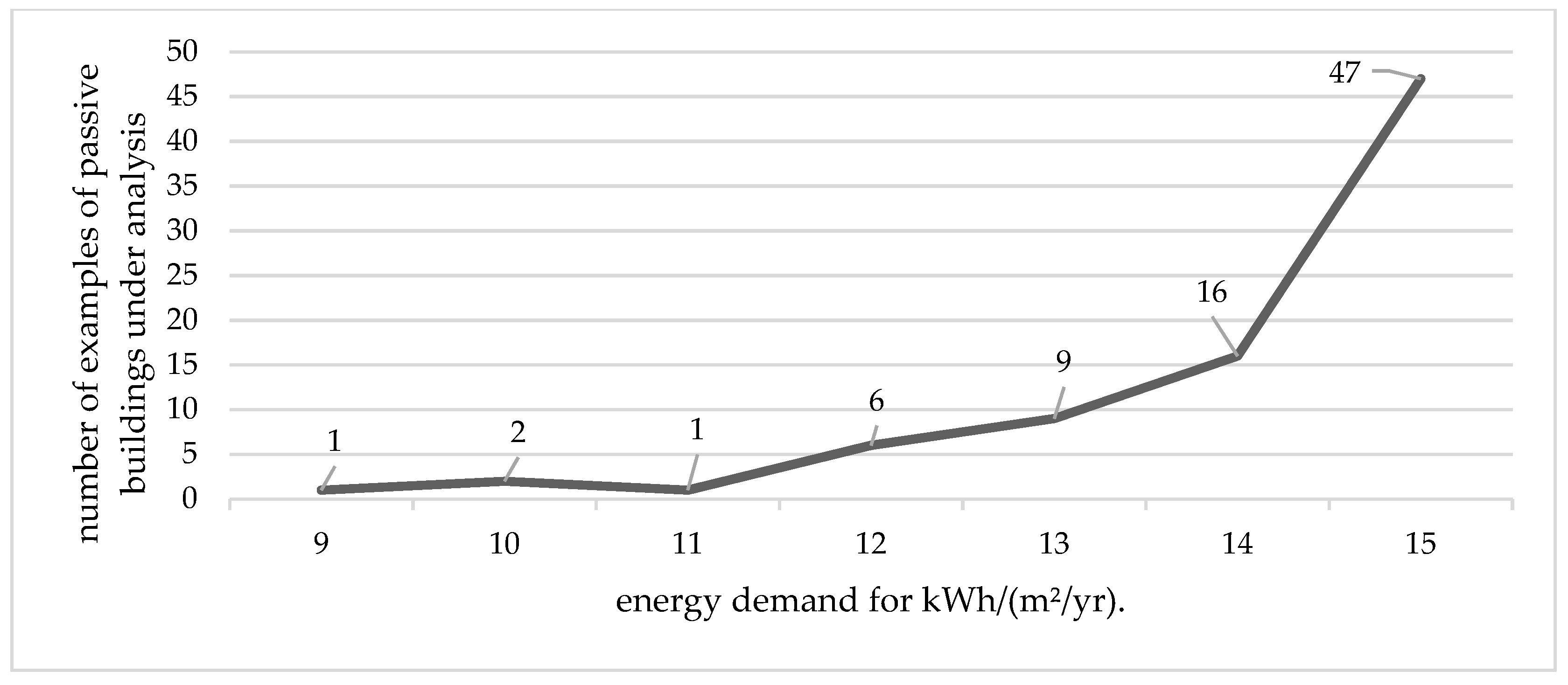
  Passive buildings with a maximum energy demand for heating of 15 kWh/(m²-yr). The selected examples have been verified by the Passive House Database (passivehouse-database.org) (Figure 2);

  ○

  Buildings with residential functions—100%;

  ○

  Number of building stories—low, up to 2 stories with attic (Figure 3).

• Territorial scope of the research includes the analysis of buildings with residential functions, implemented in Central Europe. This scope was specified to countries located in a transitional and intermediate warm climate zone (Figure 4).
• Temporal range of the study refers to passive buildings constructed between 2001 and 2017 (Figure 5). The dates refer to the final stages of the implementation, whereas the dates of conceptual or construction projects are not considered.

2.3. Method of Depth of Ground Freezing Determination

The freezing of the soil during the winter time is one of the climatic phenomena that must be taken into account when designing structures placed in the ground or the foundations of a structure [25]. Ground freezing is a multidimensional, nonstationary random process. It depends on randomly variable external and climatic phenomena, and on partially constant and partly randomly variable conditions, under the influence of external conditions as well as soil properties [26,27]. Randomly variable external conditions include primarily: air temperature and snowfall, forming snow cover on the ground [28], as well as wind speed affecting this cover and rainfall, especially before the beginning of ground freezing, as the ground humidity depends on these factors [29,30]. Additionally, the air temperature before the cold season has an impact on ground freezing because it shapes its initial temperature. The transformation of snow cover on the ground under the influence of external factors, air temperature, precipitation, and wind is also random [31,32].

The depth to which the ground freezes is most often identified with the position of the zero isotherm in the ground. In addition to external factors, freezing obviously depends on the soil type, its consistency, composition, and water content. Therefore, the freezing depth is not always the same as the position of the zero isotherm. Since meteorological stations measure ground temperature (for the last 50 years) and on this basis determine the position of the zero isotherm, it is considered here as the freezing depth. Following the measurements performed by the meteorological stations of the Institute of Meteorology and Water Management—National Research Institute, data on ground temperature were collected, allowing their probabilistic analysis and providing proposals for changes on the standard map of ground freezing. The soil freezing depth can be determined using a number of direct approaches, for example, by direct measurement using thermometers installed in the ground [33,34]. In Poland, soil temperature is measured daily in the meteorological stations.

The freezing depth may be estimated using numerical or analytical modeling techniques [34,35,36]. These methods require a large amount of input data: for example, thermal properties of materials, water content, air temperature, solar radiation, precipitation, wind velocity, etc. In most cases, input data are either not available or expensive to collect. In the case of missing data, higher or similar accuracies may be obtained from simpler analytical and semiempirical models (e.g., Stefan model, modified Berggren model, or Chisholm and Phang empirical model [36,37]). However, it is obvious that the penetration of frost into the ground is a complex and random process in which many factors affect the final results that often diverge from the observations. All climatic conditions are of random character and should be analyzed using probabilistic methods [38]. The forecast values of the position of the zero isotherm in the ground are calculated by approximations of the empirical values of the maximum annual (winter) values with a selected probability distribution. As with other climatic interactions, the Gumbel distribution [39] is well suited for this. Its distributive function is represented by the formula:

$$F\left(Z\right)=exp\left\{-exp\left[-\alpha \left(Z-U\right)\right]\right\}$$

(1)

where α and U are the distribution parameters.

This distribution and procedure have been widely used to e.g., forecast wind velocity and snow load [40]. They were also used to forecast soil freezing [41]. After being doubly logarithmized, the formula takes the form of a linear function with respect to α, U. Value Z_k of the depth of zero centigrade temperature and the 50-year return period is calculated using the following equation:

$$Z=U-\frac{1}{\alpha }ln\left[-lnF\left(Z\right)\right].$$

(2)

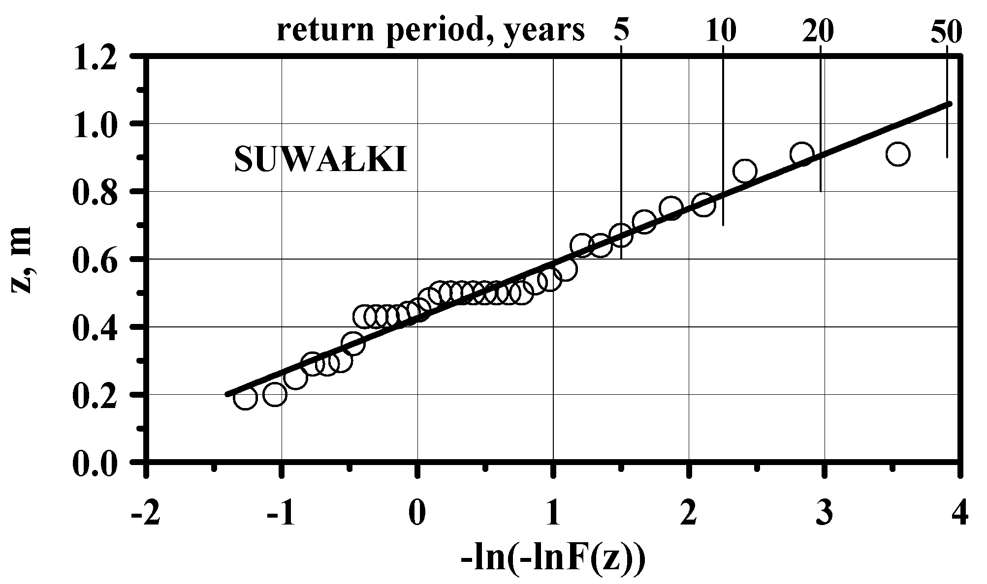
This property allows for easy construction of the so-called Gumbel probability grid on which an empirical distributive can be presented and compared with a simple equation (Figure 6).

The unknown Gumbel distribution parameters (α, U) can be estimated using the least squares method, the maximum likelihood method, the moment method, and the method described by Julius Lieblein [42]. Lieblein proposed a method of estimating Gumbel distribution parameters based on order statistics, requiring the sample elements Z_i to be placed in ascending order. The estimators of the investigated distribution parameters take the form of a linear function with respect to positional statistics:

$${\widehat{b}}_{\left(n\right)}=\frac{1}{{\widehat{\alpha }}_{\left(n\right)}}={\displaystyle \sum }_{i=1}^n{b}_i{Z}_i,\widehat{U}={\displaystyle \sum }_{i=1}^n{a}_i{Z}_i$$

(3)

where Best Linear Unbiased Estimators (BLUE) are with minimal variance. The coefficients b_i, a_i were collated in the paper [42] for a sample size of n = 1,2,…,16. The aforementioned work also describes a method of estimating parameters $b,U$ for an arbitrarily large sample with a size of n having given coefficients for an m-element sample if m < n. For an n-element sample, the coefficients $b_i^{\prime },a_i^{\prime }$ can be calculated using the following formulas:

$$\begin{array}{l}{b}_i^{\prime }={\displaystyle \sum _{j=1}^m}{b}_j\cdot \left(\frac{j}{i}\right)p\left(n,m,i,j\right),\\ i=1,2,\dots ,n\\ a_i^{\prime }={\displaystyle \sum _{j=1}^m}{a}_j\cdot \left(j/i\right)p\left(n,m,i,j\right),\end{array}$$

(4)

where:

$$p\left(n,m,i,j\right)=\left(\begin{array}{c}i\\ j\end{array}\right)\left(\begin{array}{c}n-i\\ m-j\end{array}\right)/\left(\begin{array}{c}n\\ m\end{array}\right)$$

(5)

is the hypergeometric probability function. The formulas below allow the calculation of “good” estimators ${\widehat{b}}_{\left(n\right)}^{\prime }, {\widehat{U}}_{\left(n\right)}^{\prime }$ for an n-element sample:

$$\begin{gathered} {\widehat{b}}_{\left(n\right)}^{\prime }=\frac{1}{{\widehat{\alpha }}_{\left(n\right)}^{\prime }}={{\displaystyle \sum }}_{i=1}^n{b}_i^{\prime }\cdot Z_i,{\widehat{U}}_{\left(n\right)}^{\prime }={{\displaystyle \sum }}_{i=1}^n{a}_i^{\prime }\cdot Z_i \\ {b}_{\left(i\right)}^{^"\prime }={\displaystyle \sum }_{j=1}^m{b}_j\cdot \left(\frac{j}{i}\right)p\left(n,m,i,j\right), \end{gathered}$$

(6)

The samples analyzed in this work contain significantly more than 16 measurement results; therefore, a set of BLUE coefficients b_j, a_j for m = 16 was used in the calculations.

The evaluation of the results obtained with four methods proved to be more difficult than the estimation of the Gumbel distribution parameters. As we have four Gumbel distributions, we face the question of which of them best approximates the empirical distribution and can be used to determine the characteristic value Z_k of the location of the zero isotherm in the ground [31]. The test statistics of chi-squared, Kolmogorov–Smirnov, and Cramer von Mises were adopted as a measure of adjustment of the theoretical to the empirical distribution. Low values of these statistics indicate that the given theoretical distribution truly reflects the empirical distribution.

Amid the known compliance tests, the chi-squared test is mentioned first. It requires the decomposition of the Z axis into $r+1$ intervals $I_1, I_2, \dots ,I_{r+1}$ by the numbers $-\infty =g_0<g_1<\dots <g_r<g_{r+1}=\infty$. The difference in the value of the cumulative distribution function F at the ends of the interval is equal to the probability p that the random variable Z will take a value belonging to that interval:

$$p_j=F\left(g_j\right)-F\left(g_{j-1}\right),j=1,2,\dots ,r+1$$

(7)

The chi squared test statistic for a measurement sequence consisting of n maximum freezing depths is given by the formula:

$${\chi }^2={\displaystyle \sum }_{j=1}^{r+1}\frac{{\left(n_j-n{p}_j\right)}^2}{n{p}_j}$$

(8)

where n_j—the number of measured values of Z within I_j, while np_j—is the expected number of measurement results which, according to the considered distribution, should be in I_j [41]. An examination of distribution compliance by means of statistics (8) leaves the choice of the number of intervals I_j into which the Z-axis is divided and the points g_j constituting the limits of these intervals. In this work, because of the ambiguity, the mentioned chi-squared test was implemented in two variants. The first one assumes the division of the Z variable axis into one-element intervals, the limits of which are arithmetic means of two values adjacent in the order statistics. The only exception here are points g₀, g_r+1 equal to minus and plus infinity, respectively. In the second variant, the division into five intervals with equal probability p_j was used. Point g₁ was set as the arithmetic mean of the fifth and sixth elements in a series of ascending order data: g₁ = (Z₅ + Z₆)/2. The value of the cumulative distribution function at point g₁ is equal to the probability of the first interval: F(g₁) = p. The same probability of all intervals is ensured by the next boundary points g_j being defined as:

$$g_j=U-\frac{1}{\alpha }ln\left[-ln\left(p+F\left(g_{j-1}\right)\right)\right],j=1,2,\dots ,r$$

(9)

except the last: $g_{r+1}=\infty$.

Other tests refer to the hypothetical cumulative distribution function and verify its compliance with the empirical cumulative distribution function. The Kolmogorov–Smirnov statistics D_n1 verifies the quality of the adjustment on the basis of the largest absolute value of the hypothetical F(Z) and empirical F_n(Z) cumulative distribution function difference:

$$D_{n1}=\underset{z}{sup}\left|F_n\left(Z\right)-F\left(Z\right)\right|.$$

(10)

In Formula (16), unlike in (15), the $\sqrt{n}$ factor is omitted, because only equally numerous sets of values $F_n\left(Z\right)$ and F(Z) are compared with each other and without any reference to samples of a different size n. Another variation of Kolmogorov–Smirnov statistics found in the literature was also used, namely:

$$D_n^{+}=\underset{1\le i\le n}{max}\left|\frac{i}{n}-F\left(Z_{i:n}\right)\right|,D_n^{-}=\underset{1\le i\le n}{max}\left|F\left(Z_{i:n}\right)-\frac{i-1}{n}\right|$$

(11)

from where:

$$D_{n2}=max\left\{D_n^{+},D_n^{-}\right\}.$$

(12)

The above Formulas (10)–(12) define the maximum discrepancy between the postulated Gumbel distribution and the measured depths of the zero isotherm location. So, the idea arose to do a similar check for medium differences of hypothetical and geometrical cumulative distribution function. The subsequent tests are equivalent to statistics (10)–(12) and check not the maximum but rather the average distance of the hypothetical and empirical cumulative distribution function. According to this reasoning, statistics (10) representing the average spacing of the cumulative distribution function is given by the formula:

$$D_{n1s}={\displaystyle {{\displaystyle \sum }}_{i=1}^n}\frac{\left|F_n\left(Z_i\right)-F\left(Z_i\right)\right|}{n}.$$

(13)

Whereas the equivalent of statistics (18) in relation to the average value is expressed by the formulas:

$$D_n^{+}=\frac{1}{n}{\displaystyle \sum }_{i=1}^n\left|\frac{i}{n}-F\left(Z_{i:n}\right)\right|,D_n^{-}=\frac{1}{n}{\displaystyle \sum }_{i=1}^n\left|F\left(Z_{i:n}\right)-\frac{i-1}{n}\right|$$

(14)

and next:

$$D_{n2s}=\frac{1}{2}\left(D_n^{+}+D_n^{-}\right).$$

(15)

Another test used in this work, comparing the cumulative distribution function with order statistics of measurement results, is Cramer von Mises’s statistics [41] in the form:

$$W_{CM}=\frac{1}{12n}+{\displaystyle {{\displaystyle \sum }}_{i=1}^n}{\left(F\left(Z_i\right)-\frac{2i-1}{2n}\right)}^2.$$

(16)

The best estimation method was considered to be the one indicated by most of the mentioned tests. For example, if the chi-squared statistic is the smallest for the Gumbel distribution parameters $\alpha ,U$ determined by the maximum likelihood method, it means that the chi-squared test indicates the maximum likelihood method as the best of four applied methods. More detailed information on the calculations performed with different estimation methods is provided in [41].

2.4. Selection of the Joint of Slab-on-Ground Foundation and External Wall to Analysis

A detailed analysis of the foundations in Appendix A indicated the two most frequently recurring solutions (Figure 7). The most frequent solution 88% is the design with a foundation slab. A further division of this solution is into: scheme 1A (Figure 7), where the foundation slab is flushed with the foundation wall (61%), and scheme 1B (Figure 7), where the foundation slab extends beyond the wall face by the thickness of the foundation wall thermal insulation at 20–30 cm (27%). The second most common solution scheme 2 (Figure 7) for building foundations is strip footing, which was used in 22% of the samples analyzed.

Designing buildings according to the PH standard has brought significant changes in the way of implementing building foundations. For a long time, the problem of heat loss through the foundations to the ground was not analyzed sufficiently [22]. Experts estimate that improper isolation of the building foundations may result in energy loss at the level of 5–15% heat loss from the entire building, depending on the climate zone in which the designed building is constructed. Therefore, the correct thermal insulation of all margins of the basement walls, foundation walls, and building foundations is a crucial task. One of the basic and most difficult responsibilities is to maintain the continuity of thermal insulation in the building foundations. In this case, the foundation slab is checked more extensively for low-energy and passive buildings, which leads to a minimum limit on the presence of thermal bridges [22,23]. The foundation slab does not require traditional excavation and, in contrast to the foundation bench (in the Polish climate zone), does not require an appropriate depth depending on the ground freezing level (80–140 cm in Poland it). Based on the statistics data collected in Appendix A, a variant of the joint of the slab-on-ground foundation and external wall according to the Scheme 1A was selected for numerical analysis, and taking into account the fact of different depths of ground freezing, a specific solution as shown in Figure 8 was proposed.

2.5. Description and Validation of the Heat-Transfer Model

When constructing non-basement buildings, the problem of ground freezing below the margin of the floor slab should be analyzed. Depending on the freezing depth for a specific climate zone, it often happens that the slab is placed above the freezing level, which in turn results in its exposure to low temperatures. The freezing zone runs along the perimeter from the building slab margin; therefore, the slab margin should be properly insulated. The solutions may be different. Their selection depends on the specific conditions that occur on the construction site. Various examples can be found in [24,43,44]. The calculation results and analysis of the value of the linear heat transfer ${\psi }_g$ and the temperature $f_{Rsi}^{2D}$ coefficients for the details proposed, with regard to the connection between the foundation slab with the external wall, were made based on the following standards: (i) PN-EN ISO 10211:2017 [45], (ii) PN-EN ISO 13370:2017 [46,47], (iii) PN-EN ISO 6946:2017-10 [48], and (iv) PN-EN ISO 13788:2013-05 [49]. The ${\psi }_g$ coefficient value depends on the configuration of the analyzed node and the U heat transfer coefficients of the wall and slab.

The dimensions of the calculation model presented in Figure 9 were adopted following PN-EN ISO 10211:2017.

The slab level is higher than the ground outside; therefore, the ${\psi }_g$ coefficient value can be determined from Formula (17) or (18).

$${\psi }_g=L_{2D}-h_w·U_w-0.5·B·U_{fg;sog}$$

(17)

$${\psi }_g=L_{2D}-\left(h_w+h_f\right)·U_w-\left(0.5·B+d_{w;e}\right)·U_{fg;sog}$$

(18)

where

$U_w$—heat transfer coefficient of the wall above the ground;

$U_{fg;sog}$—heat transfer coefficient of the floor slab;

$L_{2D}$—thermal coupling coefficient;

$h_w$—minimum distance from the connection to the cross-section plane;

$h_f$—elevation of the upper surface of the floor slab above ground level;

$d_{w;e}$—wall width above the ground.

Formula (17) uses internal dimensions, and Formula (18) uses external dimensions.

To determine the amount of heat loss, the value of the heat transfer coefficient of the slab on the ground was calculated, combining with the ground effect $U_{fg,sog}$. For this purpose, the value of the equivalent thickness of the floor $d_f$ was calculated from Formula (19). The equivalent thickness for the floor represents the depth of the ground that has the same thermal resistance as the walls.

$$d_f=d_{w;e}+{\lambda }_g·\left(R_{si}+R_{f;sog}+R_{se}\right)$$

(19)

where

${\lambda }_g$—ground thermal conductivity coefficient;

$R_{f;sog}$—thermal resistance of the floor plate.

The floor is well insulated; therefore, the $U_{fg,sog}$ coefficient was calculated to form the formula presented below:

$$U_{fg,sog}=\frac{{\lambda }_g}{0.457·B+d_f}.$$

(20)

The value of the thermal coupling coefficient

$L_{2D}$ was determined with the following formulas:

$$L_{2D}=\frac{\mathsf{\Phi }}{\mathsf{\Delta }T}$$

(21)

where

$\mathsf{\Phi }$—heat flux determined in FEM analysis;

$\mathsf{\Delta }T$—temperature difference between the external and internal environment.

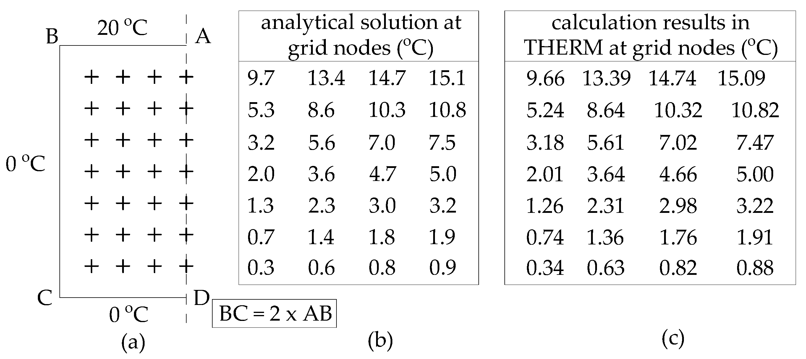
The numerical model of the two-dimensional heat-transfer effect in the analyzed node has been developed based on the finite-element method (FEM) in THERM 7.7 software. The software automatically divided cross-sections into a mesh made up of non-overlapping elements using the Finite QuadTree method. After defining the cross-section’s geometry, material properties, and boundary conditions, THERM meshes the cross-section, performs the analysis, runs an error estimation, refines the mesh if necessary, and at the end has returned the converged solution. The validation of the calculation method in the THERM 7.7 software was carried out in accordance with Annex C to the PE-EN 10211:2017 standard. For this purpose, two reference tests were carried out. For validation test case 1, the heat transfer through half a rectangle column with known surface temperatures was determined and compared to those calculated analytically and shown in Annex C of PE-EN 10211:2017 (see Figure 10b).

To perform the test, the following variables were chosen: BA = 200 mm, BC = 400 mm, thermal conductivity 0.10 W/mK, and in order to approximate the surface resistance 0 m²K/W, the highest possible film coefficient was defined in part of the boundary conditions. To ensure that THERM would calculate the temperatures at the given nodes, the model was drawn as a grid of elements with dimensions 50 mm × 50 mm: 4 elements on width and 8 elements on height. The QuadTree Mesh Parameter is set to its standard value of 6, the Maximum Percentage Error Energy Norm is set to 10%, and the Maximum Iterations is set to 5. As shown in Figure 10, the difference between the calculations in THERM and the analytical values of temperature at the 28 points of a grid does not exceed 0.1 °C.

For validation test case 2, the two-dimensional heat transfer described on the Figure 11a model was calculated. The QuadTree Mesh Parameter is set to its standard value of 6, the Maximum Percentage Error Energy Norm is set to 10%, and the Maximum Iterations is set to 5. Since all points where the temperature should be calculated are present in the geometrical model, no extra points were drawn. As shown in Figure 11b,c, the difference between the values calculated in THERM and those specified in the validation case 2 of temperature at certain points of a model does not exceed 0.1 °C. The calculated heat flow also does not differ more than 0.1 W/m from the given heat flow.

Based on the results of the simulations presented above, THERM 7.7 software complies with all the requirements of the PN-EN ISO 10211:2017 Annex C standard to be considered as a two-dimensional steady-state high-precision method.

3. Results and Discussion

3.1. Analysis of the Foundation under the Conditions of Freezing of the Ground in Poland

For the next step of the calculations, only one model of the Gumbel analysis method was used, with the best linear unbiased estimators (BLUE). These estimators are recommended in the European Standard for climate actions, e.g., the derivation of wind speeds from measurements at meteorological stations.

Using the Gumbel distribution given above, its parameters were estimated, and the calculations of the forecasted values of the zero isotherm position in the ground were performed. It was assumed that, as in the case of climatic interactions, characteristic values of the zero isotherm should have a return period of 50 years as a required reference level to ensure the reliability in design. The positions of the zero isotherm in the ground conditions of 45 meteorological stations were obtained.

Different soil types are characterized by different freezing properties. The ground freezing process consists of solar radiation, an advection of warm air masses, and the penetration of heat from deeper soil layers [41]. The freezing depth is influenced by factors related to the ground substrate, such as the soil type, its condition, degree of saturation, porosity, and mineral composition, as well as the arrangement of soil layers. Converting the obtained results into uniform ground conditions is necessary to determine the substrate conditions of the meteorological stations analyzed and establish the profile in which the temperature measurements were made. For this purpose, it is necessary to normalize and determine a reference ground, to which the results of the calculations are be compared.

If the influence of climate can be easily analyzed using the probabilistic approach, the influence of soil structure on the freezing depth is much more complex. It is due to the heterogeneity of the soil and its structure. This problem can now only be solved on the basis of the available literature using some correction coefficients. Based on these descriptions, the ground was divided into four soil types, using the results from the work of [50]. The depth of the zero isotherm for coarse and medium sands (also gravel) was taken as the basic one, introducing coefficients for other soil types and reflecting the ratios of the zero isotherm position between the mentioned soil types [31]. The subdivision given in the previous works was used here [50]. Four basic types (lithotypes) were indicated, and the following coefficients were assigned to them: gravels, coarse and medium sands—1.00; fine and silty sands—0.90; silts and sandy clays—0.80; and clays—0.70. Moreover, the above considerations do not take into account the fact that the ground at meteorological stations often consists of several different layers, which makes classification of the conditions difficult. In the absence of other data, it may be assumed that these values reflect the zero isotherm ratio between the listed soil types.

Providing a general solution of a regional nature required standardizing the substrate conditions and unifying to the reference soil. Examples of the calculation results are given in

Table 1. Results of calculations for selected localities.

Lp.	Localization	Soil Type	Conversion Coefficient for Soil Type	Gumbel Distribution Parameters for the Estimation Model: Lieblein (BLUE)		Prediction of the Zero Isotherm Position for a Return Period of 50 Years
						Results without Correction	Adjusted Results
				α	U	Z50, [m]	Z50,kor [m]
1	Białystok	FSa, siSa	0,9	5.680	0.374	1.069	1.188
2	Elbląg	Si, saCl	0,8	6.601	0.313	0.904	1.130
3	Jelenia Góra	Gr, Csa, Msa	1,0	6.291	0.303	0.924	0.924
4	Kalisz	Si, saCl	0,8	5.049	0.328	1.101	1.376
5	Koło	Cl, siCl	0,7	5.474	0.337	1.050	1.500
6	Kraków	Fsa, siSa	0,9	6.288	0.225	0.845	0.939
7	Lublin	Si, saCl	0,8	6.677	0.312	0.896	1.120
8	Łódź	Fsa, siSa	0,9	4.9232	0.392	1.184	1.316
9	Piła	Gr, Csa, Msa	1,0	4.356	0.429	1.325	1.325
10	Poznań	Si, saCl	0,8	4.148	0.444	1.385	1.731
11	Rzeszów	Gr, Csa, Msa	1,0	7.021	0.332	0.888	0.888
12	Suwałki	Si, saCl	0,8	6.092	0.405	1.046	1.308
13	Szczecin	Gr, Csa, Msa	1,0	5.088	0.253	1.020	1.020
14	Warszawa	Fsa, siSa	0,9	5.236	0.405	1.151	1.279
15	Włodawa	Fsa, siSa	0,9	4.212	0.459	1.385	1.539
16	Zielona Góra	Gr, Csa, Msa	1,0	3.699	0.374	1.429	1.429

.

From all the values of the zero centigrade position recorded during the winter season, the maximum depth was extracted and used in probabilistic calculations. This climate change may variously affect precipitation patterns due to local geographic influences. In turn, this has had an impact on conditions related to the geotechnical settings of the building foundation. Therefore, on the basis of the results obtained, a map was created. An isoline map was developed on the basis of data (1981–2011) obtained from the estimation of probability distribution parameters using Lieblein’s best linear unbiased estimators (BLUE), with the isolines estimated using the kriging method (Figure 12).

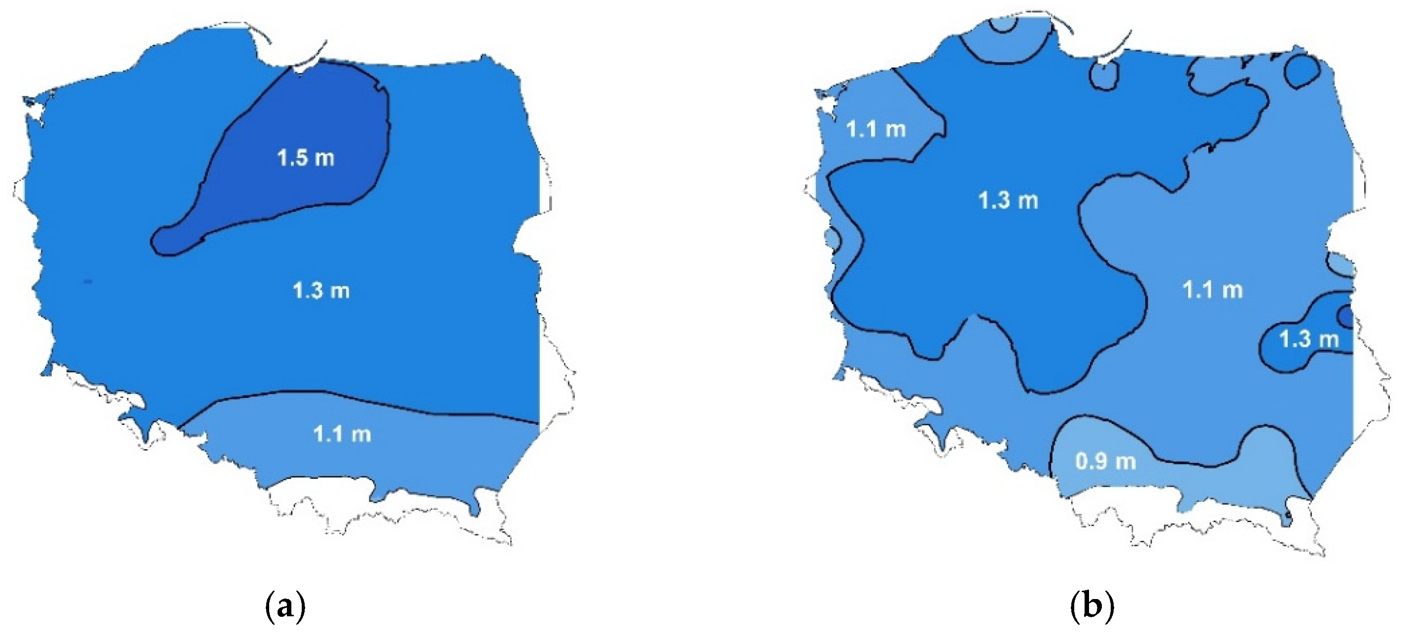
The results of our analysis indicate the possibility of establishing four freezing zones, three with values similar to those of the previous standard: 1.0 m, 1.2 m, and 1.4 m, and a mountainous zone with a value depending on the altitude above sea level but not less than 1.0 m. However, it should be noted that the given values contain a certain safety reserve due to the accepted return period (50 years); therefore, they can be treated as design values. A visible change has been noted in the range of individual zones. These changes result from global climate change, and their dynamics can be seen in the predictions made for the next decades. Using the Gumbel distribution mentioned above, its parameters were estimated, and the values of the predicted zero isotherm position in the ground for the next four decades were calculated (Figure 13a–d).

The most recent data collected (for 2012–2020) indicate the correctness of the forecasts made so far [41]. There was no case in which the recorded values of the maximum zero isotherm position were greater than the values predicted for the return period of 5 and 10 years, which was indicated in the prediction for individual locations (stations); moreover, these values were close to the matching line on the empirical distribution grid. The results obtained indicate the need to periodically update data on ground freezing (even every 5 years). This is due to the visible and increasingly dynamic global climate change.

The currently observed snowless winters (noted in Poland and Central Europe in the last 3–4 years), with low rainfall (hydrological drought) and possible sudden waves of frost can lead to increase in the range of ground freezing, as already observed in the results of measurements and presented predictions (Figure 13d). Snow cover greatly inhibits freezing depths in soils [28], so that they can vary from year to year or spatially within a given period, solely depending on the presence or absence of a snow cover. The implications of future climate, without or with increasingly intermittent snow cover, are larger freezing depths or varying freezing depths, respectively.

However, the need to update the design assumptions regarding climate change makes us give further thought on this topic. In terms of foundation design, the optimal solution would be an algorithm that allows direct determination of the freezing depth for a given location, considering current climate data (when available) and ground conditions. Although data on the soil type can be obtained from the documentation of soil tests, there is still no method to determine the parameters required to describe the heat flow phenomenon in the ground. In practice, such research is not carried out in geotechnical investigations; at the same time, there is no correlation (or with limited applicability) to determine these parameters. Studies are still being performed to solve this issue, which is why at the moment, general solutions (regional maps) are the only available method. However, the findings made so far, in the context of visible climate change, should be critical. The foundation design, in the case when the phenomenon of freezing affects the durability of the structure, concerns all constructions.

Conversely, in the case of passive buildings, while clearing snow from the area around the building (increasing the freezing range), determining a safe foundation level (below the freezing depth) is crucial for the optimal solution of the foundation and insulation.

3.2. Hydrothermal Analysis of the External Wall to Slab-on-Ground Connection

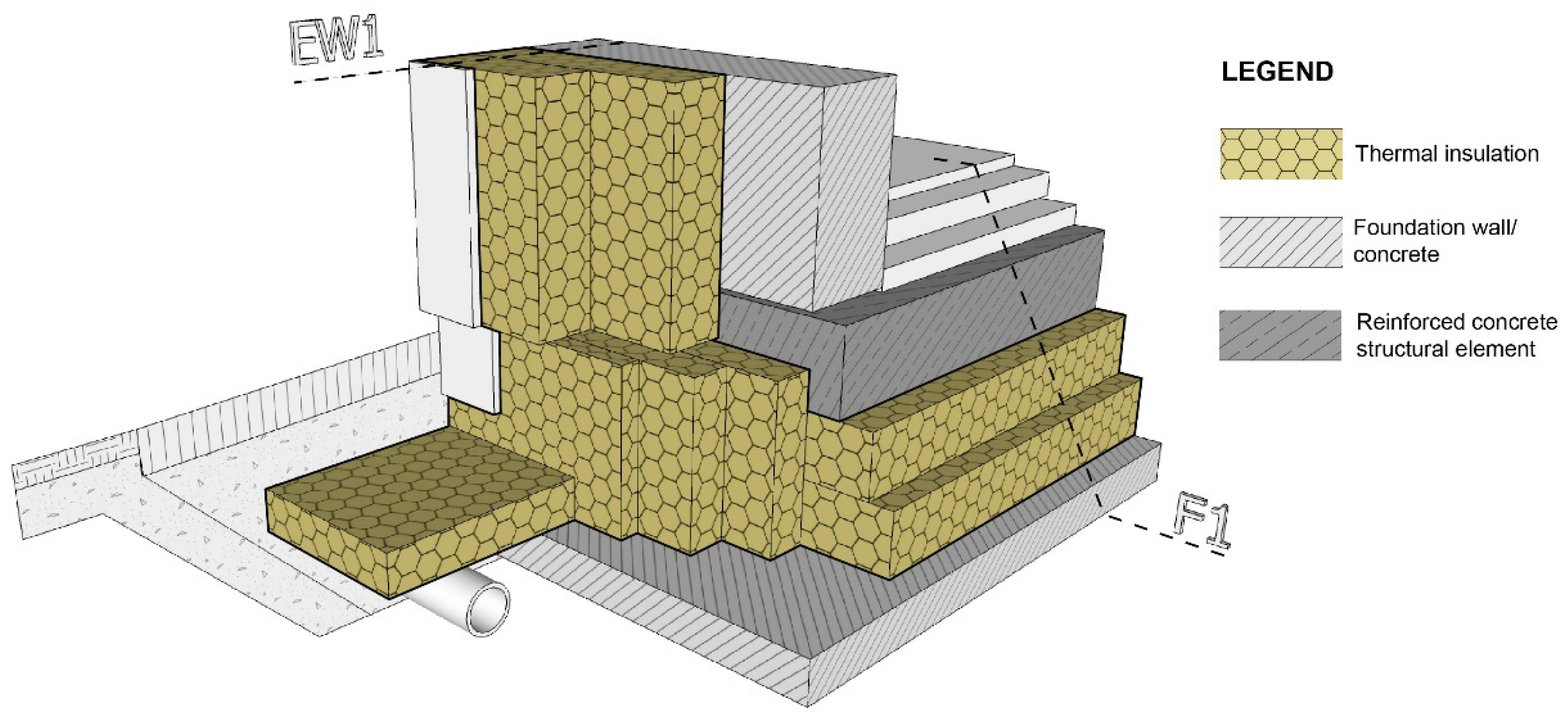
The thermal parameters of partitions included in the slab-on-ground and external wall joint proposed in Section 2.4 (Figure 8) are presented in

Table 2. U-value of heat transfer coefficient for the wall—$U_w$.

Vertical Enclosure and Horizontal Flow	Thermal Resistance
LAYERS	Thickness	λ	R
	(m)	(W/m·K)	(m2·K/W)
Outdoor environment (Rse)			0.040
Molded brick tile	0.022	0.710	0.031
Thermal isolation—graphite polystyrene	0.300	0.036	8.333
Lightweight expanded clay aggregate (LECA) block	0.240	0.191	1.257
Thin-layer gypsum plaster	0.020	0.400	0.050
Indoor environment (Rsi)			0.130
RT = Sum Ri [m2·K/W]			9.841
UT = 1/RT [W/(m2·K)]	0.10

and

Table 3. U-value of the heat transfer coefficient for the foundation slab—$U_g$.

Horizontal Enclosure and Vertical Flow	Thermal Resistance
LAYERS	Thickness	λ	R
	(m)	(W/m·K)	(m2·K/W)
Soil			-
Mechanically compacted gravel	0.450	2.000	0.225
Double compacted sand bedding	0.100	2.000	0.050
Lean concrete C12/15	0.100	1.700	0.059
Waterproofing layer	0.004	0.200	0.020
Thermal insulation—XPS 300	0.300	0.0360	8.333
Reinforced foundation slab	0.200	2.500	0.080
Thermal and acoustic insulation	0.050	0.040	1.250
Underfloor heating aluminum foil	-	-	-
Cement screed with underfloor heating	0.060	1.600	0.038
Floor—porcelain stoneware	0.040	1.000	0.040
Indoor environment (Rsi)			0.170
RT = Sum Ri [m2·K/W]			10.265
UT = 1/RT [W/(m2·K)]	0.10

. The partitions meet the thermal insulation requirements for passive buildings erected in Central Europe, as specified by the PHI ($U_w$ of the wall is equal or lower than 0.1 W/(m²·K) and $U_g$ slab-on-ground is lower than 0.14 W/(m²·K)), thus meeting the requirements from [51,52].

Two cases of the characteristic dimension $B$ were here analyzed, i.e., $B=4 \mathrm{m}$ and $B=8 \mathrm{m}$. According to PN-EN ISO 10211:2017, the calculation results for $B=8 \mathrm{m}$ apply to buildings of infinite length, while the results for $B=4 \mathrm{m}$ can be treated as representative for a single-family building. When the wall thickness $d_{w;e}=0.582 \mathrm{m}$, the ground thermal conductivity coefficient is ${\lambda }_g=2 \mathrm{W}/\mathrm{m}\mathrm{K}$. The calculations also assumed that the lean concrete below the foundation plate has the same thermal conductivity as the ground and was ignored in the calculations. The calculations also omitted the waterproofing layer and the cement screed and floor covering layer. Therefore, $R_{f;sog}=9.663 {\mathrm{m}}^2·\mathrm{K}/\mathrm{W}$, the equivalent thickness $d_f$, is equal to 20.248 m and the heat transfer coefficient of the floor plate $U_{fg,sog}=0.0837 \mathrm{W}/({\mathrm{m}}^2$K). Another important element from the point of view of the wall-slab-on-ground geometry is the level of the ground floor concerning the surrounding ground. It was assumed that this level is equal to 0.30 m. Following the guidelines of the National Fund for Environmental Protection and Water Management Priority Program, “Improving energy efficiency” [53] in which a passive building NF15 was defined, the value of the coefficient ${\psi }_g$ was determined from Formula (2) using external dimensioning. For comparison,

Table 4. Results of linear calculations of the overall heat transfer coefficient.

Property		Case
Name	Denotation/Units	B = 8 m	B = 4 m
Heat flux	$\mathsf{\Phi },\mathrm{W}$	18.7786	13.4397
% Error energy norm	%	3.99	4.88
Thermal coupling coefficient	$L_{2D},$W/K	0.4694	0.3360
Linear overall heat-transfer coefficient acc. (2)	${\psi }_g$, W/(mK)	−0.129	−0.0951
Linear overall heat-transfer coefficient acc. (1)		−0.0153	0.0186

also presents the results using Formula (1), i.e., internal dimensioning.

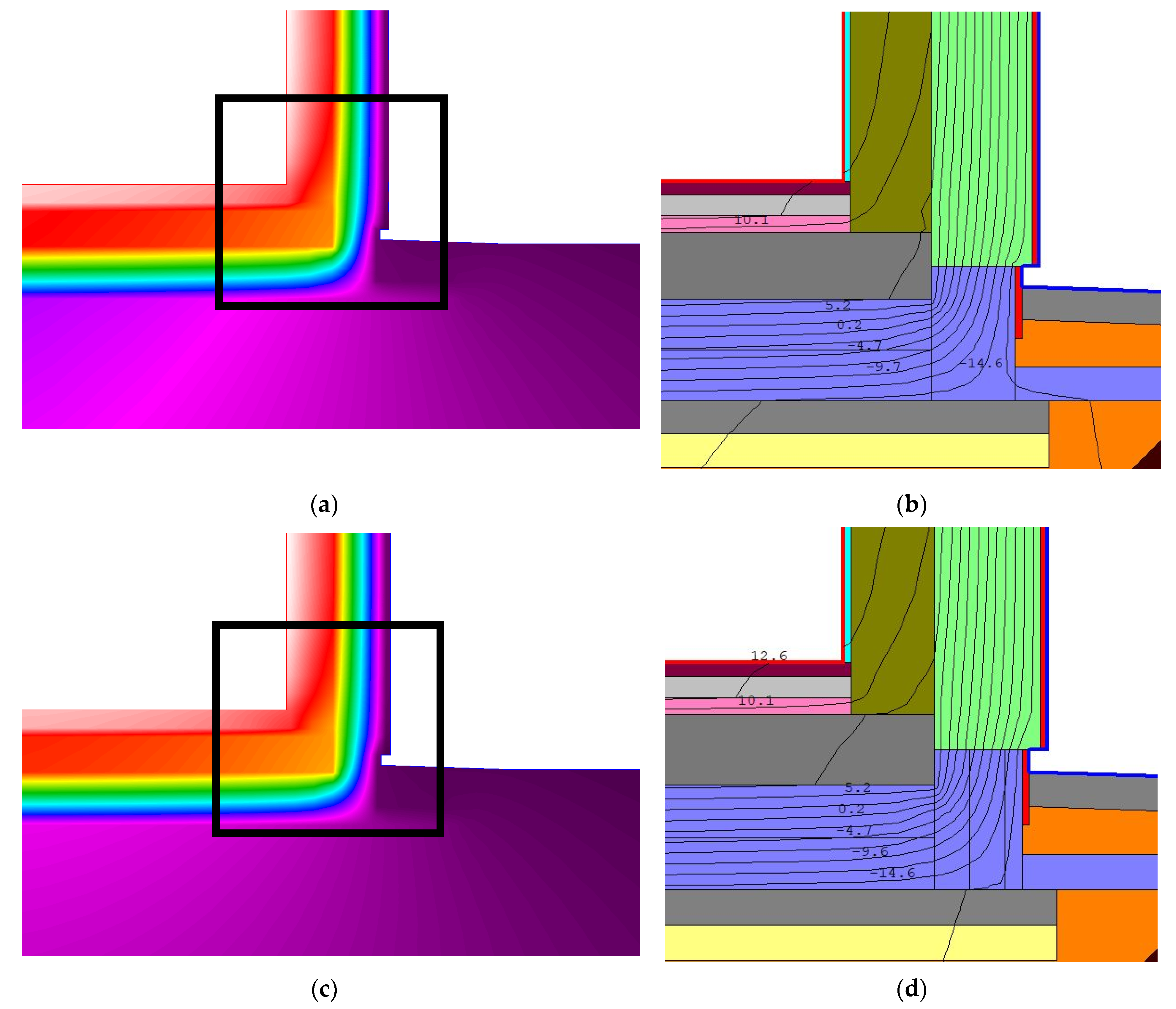
Table 4 presents detailed results for the two considered cases. Figure 14 presents the results of numerical modeling in the form of 2D temperature field distribution in a cross-section of considered details in color scale and isotherms. FEM calculations were performed in THERM 7.7. The QuadTree Mesh Parameter is set to its standard value of 6, the Maximum Percentage Error Energy Norm is set to 5%, and the Maximum Iterations is set to 25. The quadrilateral mesh was created with 1944 nodes and 1918 elements. Calculations of thermal coupling coefficient were made for the internal temperature +20 °C and external temperature −20 °C.

The linear heat transfer coefficient at the interface between the wall and the slab-on-ground determined from Formula (2) is negative in both cases. These negative values result from the connection geometry and prove the calculation of this element according to the guidelines for external dimensions. The comparison of the results of ${\psi }_g$ determined from Formulas (1) and (2) show that more favorable values are obtained in the case of external dimensioning than in the case of internal dimensioning. The values obtained for the linear heat transfer coefficient are more favorable than the default values given in the PN-EN ISO 14683:2017:-09 standard [54].

Placing on a slab is often a recommended solution for passive buildings. However, refs. [51,52] do not contain any limit values for thermal bridges. This provision is only included in the aforementioned [53] and indicates that in the area of a building foundation on the ground, the limit value of the linear heat transfer coefficient for single-family buildings in the NF15 standard is equal to 0.15 W/(mK).

This value was not exceeded for the presented solution. Furthermore, the results of the calculations show that the ${\psi }_g$ coefficient values decrease with the increase of the characteristic dimension $B$. It can be concluded that for the proposed detail of the wall to slab-on-ground connection in buildings with $B>8\mathrm{m}$, the influence of the linear bridge of the wall to slab-on-ground connection may be neglected.

The second parameter of thermal bridges that determines the suitability of a given solution in certain hygrothermal conditions is the dimensionless temperature coefficient $f_{Rsi}^{2D}$. The value of this factor should exceed 0.72. Verification of this condition allows establishing whether the analyzed construction detail was designed as to avoid the risk of vapor condensation on its internal surface. The temperature factor on the internal surface for 2D calculations is determined from Formula (22) per [45].

$$f_{Rsi}^{2D}=\frac{{\mathsf{\theta }}_{si}-{\mathsf{\theta }}_e}{{\mathsf{\theta }}_{int}-{\mathsf{\theta }}_e}$$

(22)

where

${\mathsf{\theta }}_{si}$—temperature on the internal surface in °C;

${\mathsf{\theta }}_{int}$—temperature of internal air in °C;

${\mathsf{\theta }}_e$—temperature of external air in °C.

The value of the temperature coefficient $f_{Rsi}^{2D}$ was determined for points with the lowest surface temperatures. These values were read from FEM models.

The calculation results are presented in

Table 5. Results of temperature coefficient calculations.

Property		Case
Name	Denotation/Units	B = 8 m	B = 4 m
Lowest temperature on the surface	$\mathrm{t}, °\mathrm{C}$	12.6	12.6
Temperature factor on the internal surface	$f_{Rsi}^{2D}$, -	0.815	0.815

.

Regarding the durability of the slab structure, it is important to note that in the proposed solution, the thermal insulation is arranged in such a way that no negative temperatures appear on the foundation slab (Figure 14).

The presented hygrothermal analysis confirms the possibility of recommending the analyzed solution of the wall-to-slab-on-ground for use in passive buildings in Poland, regardless of the climatic zone.

4. Conclusions

The primary task of designed foundations of single-family houses in typical projects is to transfer the weight of the building and all loads affecting the building (e.g., weight of people, equipment, snow, and wind load), to the ground. However, in the case of designing foundations for PH, it is also necessary to provide appropriate thermal isolation and minimize thermal bridges that cause heat losses [55]. Well-insulated PH foundations improve the overall energy efficiency of the building, reducing costs and energy demand while at the same time improving the thermal comfort in the building [56]. The factor of energy consumption is especially important for Polish realizations, where maintaining the passive building standard in the long term is a difficult task, being affected by people’s behavior and the type of primary energy source [57]. According to the conclusions of Grygierek’s work, scientists’ predictions of global warming should be considered in the design process of buildings for thermal isolation thicknesses [58]. As a result, a designed building with a lower primary energy demand will reduce the consumption of natural resources and reduce CO₂ emissions into the atmosphere [59,60,61].

The literature and case study analysis of foundations of passive single-family buildings in Central Europe indicated the direction and current methods of PH foundations under similar climatic conditions in Poland. At the same time, it should be noted that Polish passive building designers follow also the design practice and experience of their colleagues from the bordering countries. Therefore, the developed model of the building foundation (Section 2.4) does not differ significantly from the details of, e.g., German buildings. However, the designed model of the foundation of a PH that could be realized in Poland should consider: (i) available construction materials, (ii) ground freezing depth in Poland, (iii) climatic conditions such as temperature and rainfall.

In terms of the approach for ground freezing prediction, the obtained results indicate that the existing map should be changed, as it was developed on the basis of calculations using approximate formulas taking into account only air temperature. Probabilistic analysis of ground temperature takes into account the random nature of the phenomenon and the contribution of not only air temperature but also snow cover as well as water content in the ground resulting from previous rainfall, before frost occurrence. More research on the influence of soil structure on freezing is needed. Such investigations should be carried out for different soil types. They should also examine the difference between the depth of the zero centigrade position and the actual penetration of frost into the soil. Meanwhile, correction coefficients should be used as presented above. The presented results of the freezing depth prediction for subsequent decades indicate the intensity of climatic changes and thus the need for cyclical verification of the assumptions.

Due to the fact of very different freezing depths in Poland, which was proven in the article, a good solution in the context of passive buildings in this climate zone is to use a slab-on-ground foundation in the proposed variant of connection with the external wall. The hygrothermal analysis proved that from the point of view of the durability of the structure in the presented solution, the thermal insulation is arranged in such a way that there is no negative temperature in the slab itself. A foundation below the freezing zone would significantly increase the costs of building a passive house, and it would be difficult to exclude thermal bridges. Most of the newly designed single-family buildings in Poland do not have a basement, which means that a slab on the ground can be used as a foundation. The slab-on-ground foundation has the advantage that its position does not have to be at the depth determined by the depth of the freezing zone. The combination of the foundation slab structure with the underfloor heating system prevents the penetration of moisture into the concrete and stabilizes the temperature in the house.

References

- Cotterell, J.; Dadeby, A. The Passivhaus Handbook: A Practical Guide to Constructing and Retrofitting Buildings for Ultra-Low-Energy Performance; UIT/Green Books: Cambridge, UK, 2013; ISBN 978-0-85784-019-6. [Google Scholar]
- Hopfe, C.J.; McLeod, R.S. The Passivhaus Designer’s Manual: A Technical Guide to Low and Zero Energy Buildings; Routledge: New York, NY, USA, 2015; ISBN 978-0-415-52269-4. [Google Scholar]
- Moreno-Rangel, A. Passivhaus. Encyclopedia 2021, 1, 5. [Google Scholar] [CrossRef]
- Feist, W. Active for More Comfort: Passive House; International Passive House Association: Darmstadt, Germany, 2018; Available online: https://passivehouse-international.org/upload/Passive_House_Active_for_more_comfort_brochure.pdf (accessed on 20 November 2021).
- Juchniewicz-Lipiñska, L. The First Certified Passive House in Poland. Architectus 2008, 2, 75–79. [Google Scholar]
- Hyde, R. Bioclimatic Housing: Innovative Designs for Warm Climates; Earthscan: London, UK, 2008; ISBN 978-1-84407-284-2. [Google Scholar]
- Piraccini, S.; Fabbri, K. Building a Passive House: The Architect’s Logbook; Springer International Publishing: Cham, Switzerland, 2018; ISBN 978-3-319-69938-7. [Google Scholar]
- Feist, W.G.; Peper, S.; Kah, O.; von Oesen, M. Climate Neutral Passive House Estate in Hannover- Kronsberg: Construction and Measurement Results; Passivhaus Institut: Darmstadt, Germany, 2005; Available online: https://passiv.de/downloads/05_cepheus_kronsberg_summary_pep_en.pdf (accessed on 20 November 2021).
- Figueiredo, A.; Rebelo, F.; Castanho, R.A.; Oliveira, R.; Lousada, S.; Vicente, R.; Ferreira, V.M. Implementation and Challenges of the Passive House Concept in Portugal: Lessons Learnt from Successful Experience. Sustainability 2020, 12, 8761. [Google Scholar] [CrossRef]
- Dequaire, X. Passivhaus as a Low-Energy Building Standard: Contribution to a Typology. Energy Effic. 2012, 5, 377–391. [Google Scholar] [CrossRef]
- Peper, S.; Feist, W. Energy Efficiency of the Passive House Standard: Expectations Confirmed by Measurements in Practice; Passive House Institute: Darmstadt, Germany, 2015; Available online: https://passiv.de/downloads/05_energy_efficiency_of_the_passive_house_standard.pdf (accessed on 20 November 2021).
- Schnieders, J.; Feist, W.; Rongen, L. Passive Houses for Different Climate Zones. Energy Build. 2015, 105, 71–87. [Google Scholar] [CrossRef]
- Schnieders, J.; Hermelink, A. CEPHEUS Results: Measurements and Occupants’ Satisfaction Provide Evidence for Passive Houses Being an Option for Sustainable Building. Energy Policy 2006, 34, 151–171. [Google Scholar] [CrossRef]
- Feist, W. First Steps: What Can Be a Passive House in Your Region with Your Climate? 2015. Available online: http://www.solaripedia.com/files/170.pdf (accessed on 20 November 2021).
- Kočí, V.; Bažantová, Z.; Černý, R. Computational Analysis of Thermal Performance of a Passive Family House Built of Hollow Clay Bricks. Energy Build. 2014, 76, 211–218. [Google Scholar] [CrossRef]
- Mahdavi, A.; Doppelbauer, E.-M. A Performance Comparison of Passive and Low-Energy Buildings. Energy Build. 2010, 42, 1314–1319. [Google Scholar] [CrossRef]
- Pérez-Andreu, V.; Aparicio-Fernández, C.; Vivancos, J.-L.; Cárcel-Carrasco, J. Experimental Data and Simulations of Performance and Thermal Comfort in a Typical Mediterranean House. Energies 2021, 14, 3311. [Google Scholar] [CrossRef]
- Details for Passive Houses: Renovation: A Catalogue of Ecologically Rated Constructions; IBO—Österreichisches Institut für Baubiologie und -ökologie; Birkhäuser: Basel, Switzerland, 2017; ISBN 978-3-0356-0953-0.
- Waltjen, T.; Pokorny, W.; Zelger, T.; Torghele, K.; Feist, W.; Peper, S.; Schnieders, J.; Mötzl, H.; Lopez, P.M. Österreichisches Institut für Baubiologie und -ökologie (Eds.). 2., Aktualisierte und erw. Aufl.; Springer: Wien, Austria, 2008; ISBN 978-3-211-29763-6. [Google Scholar]
- Simões, N.; Serra, C. Ground Contact Heat Losses: Simplified Calculation Method for Residential Buildings. Energy 2012, 48, 66–73. [Google Scholar] [CrossRef]
- Rees, S.W.; Adjali, M.H.; Zhou, Z.; Davies, M.; Thomas, H.R. Ground Heat Transfer Effects on the Thermal Performance of Earth-Contact Structures. Renew. Sustain. Energy Rev. 2000, 4, 213–265. [Google Scholar] [CrossRef]
- Corner, D.; Fillinger, J.C.; Kwok, A.G. Passive House Details: Solutions for High Performance Design; Routledge: New York, NY, USA, 2018; ISBN 978-1-138-95825-8. [Google Scholar]
- James, M.; Bill, J. Passive House in Different Climates: The Path to Net Zero; Routledge, Taylor & Francis Group: New York, NY, USA, 2016; ISBN 978-1-138-90403-3. [Google Scholar]
- Azinović, B.; Kilar, V.; Koren, D. Energy-Efficient Solution for the Foundation of Passive Houses in Earthquake-Prone Regions. Eng. Struct. 2016, 112, 133–145. [Google Scholar] [CrossRef]
- Smith, G.M.; Rager, R.E. Protective Layer Design in Landfill Covers Based on Frost Penetration. J. Geotech. Geoenviron. Eng. 2002, 128, 794–799. [Google Scholar] [CrossRef]
- Xu, X.Z.; Wang, J.C.; Zhang, L.X. Frozen Soil Physics; Science Press: Beijing, China, 2001. (In Chinese) [Google Scholar]
- Edwards, A.C.; Cresser, M.S. Freezing and Its Effect on Chemical and Biological Properties of Soil. In Soil Restoration; Lal, R., Stewart, B.A., Eds.; Advances in Soil Science; Springer: New York, NY, USA, 1992; Volume 17, pp. 59–79. ISBN 978-1-4612-7684-5. [Google Scholar]
- Goodrich, L.E. The Influence of Snow Cover on the Ground Thermal Regime. Can. Geotech. J. 1982, 19, 421–432. [Google Scholar] [CrossRef] [Green Version]
- Nixon, J.F. (Derick) Discrete Ice Lens Theory for Frost Heave in Soils. Can. Geotech. J. 1991, 28, 843–859. [Google Scholar] [CrossRef]
- Mageau, D.W.; Morgenstern, N.R. Observations on Moisture Migration in Frozen Soils. Can. Geotech. J. 1980, 17, 54–60. [Google Scholar] [CrossRef]
- Żurański, J.A.; Godlewski, T. Seasonal Ground Freezing in Poland; Building Research Institute: Warsaw, Poland, 2017; ISBN 978-83-249-8490-9. (In Polish) [Google Scholar]
- Godlewski, T. New approach to the problem of soil freezing in Poland. Acta Sci. Pol. Arch. 2018, 17, 121–129. [Google Scholar] [CrossRef]
- Janiszewski, F. Instruction for Meteorological Stations; IMGW: Warsaw, Poland, 1988; ISBN 8322003293. (In Polish) [Google Scholar]
- Vermette, S.; Christopher, S. Using the Rate of Accumulated Freezing and Thawing Degree Days as a Surrogate for Determining Freezing Depth in a Temperate Forest Soil. Middle States Geogr. 2008, 41, 68–73. [Google Scholar]
- Rajaei, P.; Baladi, G.Y. Frost Depth: General Prediction Model. Transp. Res. Rec. 2015, 2510, 74–80. [Google Scholar] [CrossRef]
- U.S. Army and Air Force. Arctic and Subarctic Construction Calculation Methods for Determination of Depths of Freeze and Thaw in Soils; Technical Manual: TM5-852-6/AFM; Departments of the Army and the Air Force: Washington, DC, USA, 1988; Available online: https://armypubs.army.mil/epubs/DR_pubs/DR_a/pdf/web/tm5_852_6.pdf. (accessed on 20 November 2021).
- Yu, F.; Guo, P.; Lai, Y.; Stolle, D. Frost Heave and Thaw Consolidation Modelling. Part 1: A Water Flux Function for Frost Heaving. Can. Geotech. J. 2020, 57, 1581–1594. [Google Scholar] [CrossRef]
- Steurer, P.M. Probability Distributions Used in 100-Year Return Period of Air-Freezing Index. J. Cold Reg. Eng. 1996, 10, 25–35. [Google Scholar] [CrossRef]
- Gumbel, E.J. Statistics of Extremes; John Wiley & Son: Hoboken, NJ, USA, 1958; ISBN 978-0-231-89131-8. [Google Scholar]
- Żurański, J.A.; Sobolewski, A. Snow Loads in Poland in Designing and Diagnostics of Structures; Building Research Institute: Warsaw, Poland, 2016; ISBN 978-83-249-8470-1. (In Polish) [Google Scholar]
- Godlewski, T.; Wodzyński, Ł.; Wszędyrówny-Nast, M. Probabilistic Analysis as a Method for Ground Freezing Depth Estimation. Appl. Sci. 2021, 11, 8194. [Google Scholar] [CrossRef]
- Lieblein, J. Efficient Methods of Extreme-Value Methodology; Institute for Applied Technology, National Bureau of Standards: Washington, USA, 1974. Available online: https://www.itl.nist.gov/div898/winds/pdf_files/A3-3_Lieblein.pdf (accessed on 20 November 2021).
- Stolarska, A.; Strzałkowski, J. Modelling of Edge Insulation Depending on Boundary Conditions for the Ground Level. IOP Conf. Ser. Mater. Sci. Eng. 2017, 245, 042003. [Google Scholar] [CrossRef]
- Borelli, D.; Cavalletti, P.; Marchitto, A.; Schenone, C. A Comprehensive Study Devoted to Determine Linear Thermal Bridges Transmittance in Existing Buildings. Energy Build. 2020, 224, 110136. [Google Scholar] [CrossRef]
- International Organization for Standardization. PN-EN ISO 10211:2017 Thermal Bridges in Building Construction—Heat Flows and Surface Temperatures—Detailed Calculations; International Organization for Standardization: Geneva, Switzerland, 2017. [Google Scholar]
- Medved, S.; Černe, B. A Simplified Method for Calculating Heat Losses to the Ground According to the EN ISO 13370 Standard. Energy Build. 2002, 34, 523–528. [Google Scholar] [CrossRef]
- International Organization for Standardization. PN-EN ISO 13370:2017 Thermal Performance of Buildings—Heat Transfer via the Ground—Calculation Methods; International Organization for Standardization: Geneva, Switzerland, 2017. [Google Scholar]
- International Organization for Standardization. PN-EN ISO 6946:2017-10 Building Components and Building Elements-Thermal Resistance and Thermal Trans-Mittance-Calculation Methods; International Organization for Standardization: Geneva, Switzerland, 2017. [Google Scholar]
- International Organization for Standardization. PN-EN ISO 13788:2013-05 Hygrothermal Performance of Building Components and Building Elements-Internal Surface Temperature to Avoid Critical Surface Humidity and Interstitial Condensation-Calculation Methods; International Organization for Standardization: Geneva, Switzerland, 2013. [Google Scholar]
- Gontaszewska, A. Thermophysical Properties of Soil with Regard to Frost; Oficyna Wydawnicza Uniwersytetu Zielonogórskiego: Zielona Góra, Poland, 2010; ISBN 978-83-7481-315-0. [Google Scholar]
- Regulation of the Minister of Infrastructure of 12 April 2002 on Technical Conditions, Which Should Correspond to the Buildings and Their Location. Available online: http://isap.sejm.gov.pl/isap.nsf/download.xsp/WDU20190001065/O/D20191065.pdf (accessed on 20 November 2021). (In Polish)
- Regulation of the Minister of Development, Work and Technology of 21 December 2020 on Technical Conditions, Which Should Correspond to the Buildings and Their Location. Available online: https://isap.sejm.gov.pl/isap.nsf/download.xsp/WDU20200002351/O/D20202351.pdf (accessed on 20 November 2021). (In Polish)
- Priority Programme “Improvement of Energy Efficiency Part 2: Subsidies to Credits for Construction of Energy-Saving Houses”, National Fund for Environmental Protection and Water Management. Available online: http://beta.nfosigw.gov.pl/oferta-finansowania/srodki-krajowe/programy-priorytetowe/doplaty-do--kredytow-na-domy-energooszczedne/prezentacje-z-wytycznych-do-programu/ (accessed on 20 November 2021). (In Polish)
- International Organization for Standardization. PN-EN ISO 14683:2017-09 Thermal Bridges in Building Construction—Linear Thermal Transmittance—Simplified Methods and Default Values; International Organization for Standardization: Geneva, Switzerland, 2017. [Google Scholar]
- Leal, V. Buildings Energy Efficiency and Innovative Energy Systems. Energies 2021, 14, 5092. [Google Scholar] [CrossRef]
- Ferdyn-Grygierek, J.; Grygierek, K.; Gumińska, A.; Krawiec, P.; Oćwieja, A.; Poloczek, R.; Szkarłat, J.; Zawartka, A.; Zobczyńska, D.; Żukowska-Tejsen, D. Passive Cooling Solutions to Improve Thermal Comfort in Polish Dwellings. Energies 2021, 14, 3648. [Google Scholar] [CrossRef]
- Wąs, K.; Radoń, J.; Sadłowska-Sałęga, A. Maintenance of Passive House Standard in the Light of Long-Term Study on Energy Use in a Prefabricated Lightweight Passive House in Central Europe. Energies 2020, 13, 2801. [Google Scholar] [CrossRef]
- Grygierek, K.; Sarna, I. Impact of Passive Cooling on Thermal Comfort in a Single-Family Building for Current and Future Climate Conditions. Energies 2020, 13, 5332. [Google Scholar] [CrossRef]
- Mazur, Ł. Circular Economy in Housing Architecture: Methods of Implementation. Acta Sci. Pol. Arch. 2021, 20, 65–74. [Google Scholar] [CrossRef]
- Skutnik, Z.; Sobolewski, M.; Koda, E. An Experimental Assessment of the Water Permeability of Concrete with a Superplasticizer and Admixtures. Materials 2020, 13, 5624. [Google Scholar] [CrossRef]
- Sivasuriyan, A.; Vijayan, D.S.; Górski, W.; Wodzyński, Ł.; Vaverková, M.D.; Koda, E. Practical Implementation of Structural Health Monitoring in Multi-Story Buildings. Buildings 2021, 11, 263. [Google Scholar] [CrossRef]
Figure 1.
Scheme of the methodology.
Figure 2.
Analysis of passive buildings in terms of their energy demand.
Figure 3.
Analysis of passive buildings in terms of number of buildings stories.
Figure 4.
Geographic analysis of passive buildings.
Figure 5.
Temporal analysis of passive building implementation.
Figure 6.
Maximum depth of zero centigrade temperature presented on the Gumbel probability plot. Reprint with permission [31]; Copyright 2017, Building Research Institute.
Figure 7.
Schemes of the most common solutions of joint of the slab-on-ground foundation and external wall in PH.
Figure 8.
Detail of the joint of the slab-on-ground foundation and external wall. Layers: (i) EW1—external wall (ii) F1—floor on the-described in Section 3.2.
Figure 9.
Geometry of the wall- to slab-on-ground calculation model.
Figure 10.
(a) Geometry and boundary conditions for test case 1 of Annex C PN-EN ISO 10211:2011, (b) Analytical solution at grid nodes for test case 1 of Annex C PN-EN ISO 10211:2011, (c) Calculation results in THERM at analyzed grid nodes.
Figure 11.
(a) Geometry and boundary conditions for test case 2 of Annex C PN-EN ISO 10211:2011, (b) Analytical solution at grid nodes for test case 2 of Annex C PN-EN ISO 10211:2011, (c) Calculation results in THERM at analyzed grid nodes.
Figure 12.
Proposal for a new map of ground freezing in Poland with predetermined values of the zero isotherm depth (Zk) and ranges of special zones in Poland. Reprint with permission [31]; Copyright 2017, Building Research Institute [31].
Figure 13.
Changes in ground freezing zones in Poland over the last 50 years. (a) Years 1981–1990. (b) Years 1991–2000. (c) Years 2001–2010. (d) Years 2011–2020.
Figure 14.
(a) Temperature field distribution in the cross-section of the detail wall–slab-on-ground for the case where B = 8 m, (b) Isotherms in the fragment marked with a square in figure (a), (c) Temperature field distribution in the cross-section of the detail wall–slab-on-ground for the case where B = 4 m, (d) Isotherms in the fragment marked with a square in figure (c), (e) Legends.