1. Introduction
As stated by the International Energy Agency, the cleanest and most sustainable energy is that which we do not consume. Energy efficiency was first considered hidden fuel, then first fuel, and finally as having a key role to play in a clean energy transition. Moreover, energy efficiency offers several benefits, such as improving energy security, increasing employment, and reducing CO
2 emissions [
1]. However, an extended energy-efficiency gap still exists [
2]; namely, profitable energy-efficiency interventions are not implemented due to several barriers pertaining to different categories [
3] and involving enterprises of various sizes in different sectors [
4]. A wide range of policies have been developed by different countries to address the energy-efficiency gap, as shown by Tanaka in [
5]. The number of such policies steadily increased in the period from 1970 to 2011.
Energy use accounts for 75% of the EU’s emissions [
6]. The transformation of energy systems is central to achieving the European climate and energy goals reported in the European Green Deal [
7].
The European Union stresses the need to adopt a holistic approach in which all EU actions and policies contribute to the objectives of the Green Deal itself. The Commission communication announced initiatives covering several policy areas that are all highly interlinked, including climate, environment, energy, transport, industry, agriculture, and sustainable finance.
Saving more energy and using more renewable energies is a key driver for jobs, growth, and emission reduction. In this context, energy efficiency is a milestone in the industrial and tertiary transformation process. Making production processes more efficient and rationalizing the use of energy resources are the main objectives of the European Commission’s approach to the issue of energy efficiency in production processes.
The Energy Efficiency Directive 2012/27/EU (EED) [
8] (and the 2018/2002 directive amendment [
9]) is a key element of Europe’s energy legislation. It includes a balanced set of binding measures intended to help EU Member States reach the 20% energy efficiency target by 2020. The increase in energy efficiency in the production sectors turns out to be one of the cornerstones of the new European Green Deal, introduced by the European Union to reach the challenging goal of an almost global decarbonisation of the economy by 2050. As of today, in fact, industry is still responsible for 20% of greenhouse gas emissions in the EU, and to achieve this goal, a strong paradigm shift is needed in the management of production processes (from a linear model to a circular one) and in generation, distribution, and use of energy, with particular attention paid to the efficiency.
The EED establishes a common framework of measures for the promotion of energy efficiency (EE) to ensure the achievement of European targets and to pave the way for further EE improvements beyond 2020. Article 8 of the EED introduced the obligation for large enterprises to carry out an energy audit on their production sites, starting in December 2015 and subsequently every 4 years. To this extent, the Italian definition of large enterprise is a business organization with more than 250 employees and with an annual turnover exceeding EUR 50 million and/or an annual balance-sheet total exceeding EUR 43 million. The size of the enterprise takes into consideration the core company and partner/linked enterprises within the Italian territory.
In the EED, an energy audit is defined as “a systematic procedure having the purpose of obtaining adequate knowledge of the current energy consumption profile of a building or group of buildings, of an industrial or commercial operation or installation, of a private or public service, by identifying and quantifying cost-effective energy saving opportunities, and reporting the findings” [
8]. Therefore, an energy audit is the first step to characterize energetically different sites and sectors and to define a long-term strategy on energy efficiency for enterprises and policy makers.
Measuring energy-efficiency performance of equipment, processes, and factories is the first step toward effective energy management in production [
10]. In order to gain a greater awareness of energy-saving opportunities, it is necessary to compare the energy performance of a site with “market references”. In technical and scientific literature, it is not difficult to find references for single components (e.g., efficiency of air compressors [
11] or multiple energy-efficiency measures databases, including electric motors, steam generators, cooling and refrigeration systems, heat recovery, etc., promoted by the United Nations [
12], the European Commission [
13], or specific countries, such as Sweden [
14]). Moreover, there are multiple methods and tools available to assess the impact of energy-efficiency improvements in a single site or company. Some excellent reviews are focused on analysing energy assessment methods [
15], key energy performance indicators in production [
16], energy management systems in industry [
17], and energy performance indicators in ISO 50001 energy management systems [
18]. However, there is a lack of information on the definition of methods to evaluate the baseline of energy consumption in different economic sectors, which crucial information for the evaluation of the impact of energy-efficiency measures.
Energy performance indicators (or energy-efficiency indexes, EnPIs) can be based on economic data (i.e., value added by the production) or physical terms (i.e., tons or cubic meters of products), and at the sectoral level, they depend on the activity level of analysis, sector structure, and energy-efficiency maturity [
19]. Several efforts have been made to homogenise and standardise the use of multiple energy-efficiency indicators to compare energy efficiency between countries and sectors [
20]. However, currently, these methods are applied only to a limited number of energy-intensive industries (such as cement, aluminium, iron and steel, ethylene, ammonia, refining) [
21] for which the variety of final product analyses is restricted and technologies are mature [
22]. It is important to cite the efforts of the European IPPC Bureau to set up, review, and update BAT reference documents (BREFs), a series of sectoral analysis of more than 52,000 installations across Europe affected by the Industrial Emissions Directive (2010/75/EU) [
23]. These documents are the European consumption reference for several industrial processes, providing a range of EnPIs at the European level but without specific information for each country.
The energy analysis of specific economic sectors should ideally be based on physical units of production. The information must be sufficiently disaggregated to allow for the analysis of processes and sites, while models should be the same for all economic sectors [
24]. Therefore, the use of the information from energy audits is ideal to define sectoral EnPIs. Moreover, the use of linear models in energy-efficiency analysis is extensive due to their applicability in the developing benchmarks [
25], determining energy savings in industries [
26] (despite several production processes being not linear [
27]), linking energy efficiency and productivity [
28], forecasting industrial [
29] and tertiary [
30] energy consumption, evaluating benchmarks for plant indicators, as a basis for stochastic frontier analysis [
31], modelling building consumption [
32], and estimating national economic indicators of electricity consumption [
33].
Another important issue is the depth level of the description of economic activities (NACE level) in order to have a compromise between availability of data and accuracy of the information. One NACE code is assigned to enterprises or production sites according to their main economic activity. The main activity is the one which contributes most to the value added of the unit. An activity, defined by a NACE code, may consist of one simple process (for example, weaving) but may also cover a whole range of sub-processes, each mentioned in different categories of the classification (for example, car manufacturing consists of specific activities, such as casting, forging, welding, assembly, painting, etc.) [
34]. Therefore, for each NACE code, it is necessary to define clusters with homogeneous processes and/or products. Each NACE code is divided into four levels (section, division, group, and class), and it is recommended to carry out the definition of the sectoral indicators at a 4-digit NACE level (e.g., C23.51—manufacture of cement or D35.11—production of electricity) [
35].
The analysis of energy audits to define the sectoral energy performance has been investigated in scientific literature in Germany [
24,
25], Sweden [
26], Latvia [
27], the Netherlands [
28] and USA [
29]. However, a high heterogeneity of the available data has been observed, as in the methodology used in the analysis and in the obtained results.
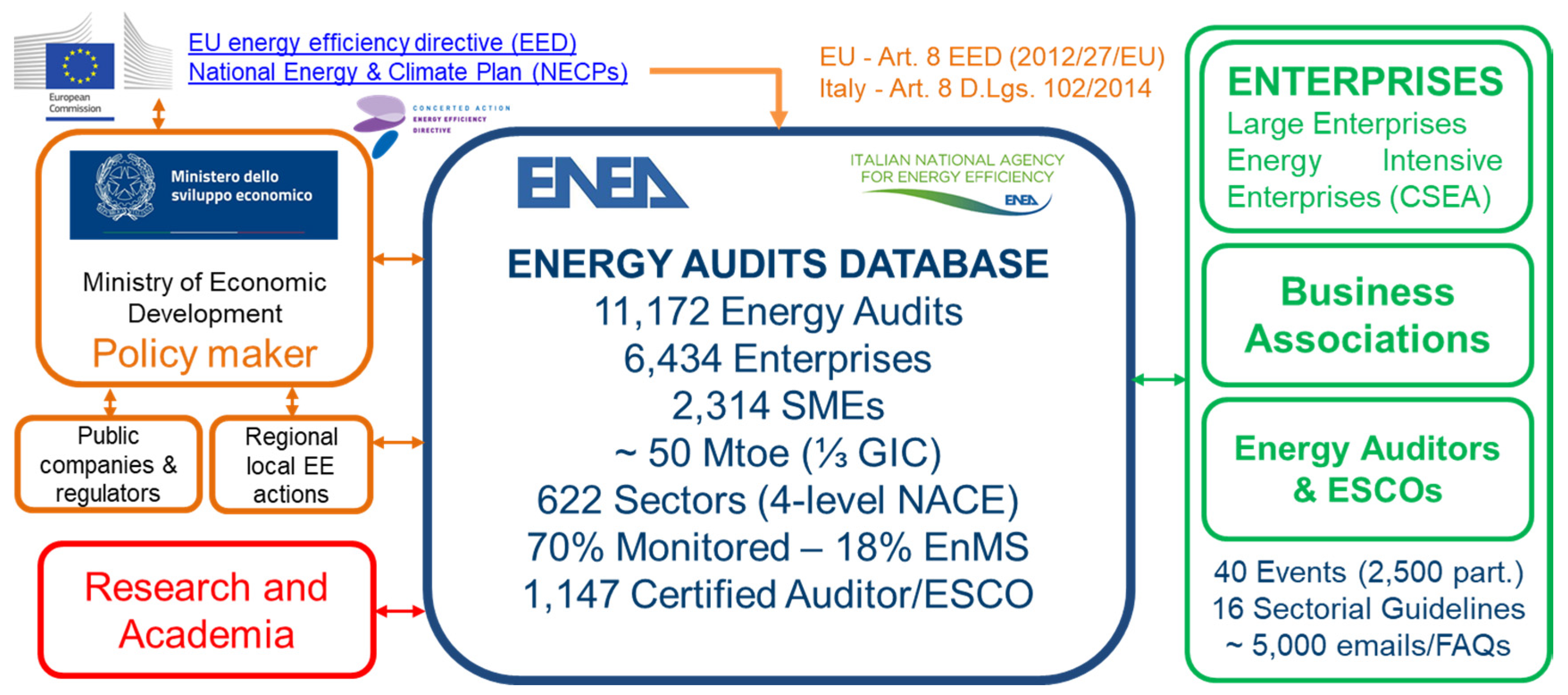
The Italian government transposed the EED in 2014 (by issuing the legislative Decree n. 102/2014, updated by legislative Decree n. 73/2020 [
36]), also extending the obligation to a specific group of energy-intensive enterprises and assigning management of EED article 8 obligations to the ENEA (Italian National Agency for New Technologies, Energy, and Sustainable Economic Development).
Energy-intensive enterprises are those with large energy consumptions (more than 1 GWh of electricity) applying for tax relief on part of the purchased energy. All energy-intensive enterprises are registered in the list of “Cassa per i servizi energetici ed ambientali” (governmental agency related to electricity) [
37].
Figure 1 shows schematically shows the Italian framework of mandatory energy audits. As of December 2019, the first deadline for the second compulsory cycle, 11,172 energy audits had been uploaded to the ENEA website from 6434 enterprises [
38].
Over 70% of the energy audits received are complemented by a monitoring plan, in accordance with the guidelines drawn up by ENEA. The presence of monitoring systems makes the available data very useful and enables an accurate and in depth analysis of sectoral consumption (energy performance indicators, sectoral analysis, energy-consumption trend evaluation) and technologies. Monitoring also makes the energy audit itself very valuable, as it makes it possible to identify energy cost centres and therefore favours the implementation of energy-efficiency measures in order to reduce energy consumption and make production processes more efficient [
39]. The Italian transposition of the NACE codes (ATECO codes) introduces two additional levels (categories and subcategories).
The purpose of this work is to identify a methodology that allows for the evaluation of EnPI values that is valid for the entire production process for all 4-digit NACE-level sectors (transposed in Italy as 6-digit ATECO-level sectors) and for the production process of an enterprise or production site. This methodology has been applied to more than 300 4-digit NACE-level sectors using the Italian database of mandatory energy audits from Art. 8 of EED, and it has been also applied to several subsectors at the process level.
This work has been developed within the framework of the research program National Electrical System Research (in Italian, “Piano Triennale della Ricerca del Sistema Elettrico Nazionale 2019–2021”), funded by the Italian Ministry of Economic Development, with the task “energy efficiency of industrial products and processes”. The main objective of this task is the analysis of the definition of best practices and performance indicators for energy-efficiency interventions based on the information from energy audits. This task has been developed in collaboration with several universities, business associations, and sectoral experts. Detailed guidelines for six industrial sectors (glass, cement, waste valorisation, ceramic, pharma, and foundries) are available in [
40].
2. Methodology
2.1. Data Collection
The Audit102 database (
https://audit102.enea.it/) stores, for every audited site, production volumes representing the activity, purchase, and consumption volumes of all energy commodities. End uses are split among three main functional areas: core activity, auxiliary services, and general services. The first two levels of the tree-structure energy model are therefore available in the database. In order to limit the effort imposed on companies and conglomerates involving multiple production sites and premises, energy audits, with the analysis of energy-performance improvement actions, may be carried out on a limited number of representative sites by using a clustering strategy. Following the sampling strategy [
41], focus is directed toward sites featuring a higher energy demand and those most likely to reward any energy saving measure with greater economic benefits. The database includes, for every audited site, information on energy performance improvement actions (EPIAs), both implemented and planned ones. EPIAs are described identifying the intervention category, which can be technical, (e.g., “pressure systems”, “heat recovery systems and thermal plant”, “inverters and other electrical machines and installations”) or managerial, such as the introduction or improvement of a monitoring system or the adoption of ISO 50001 certification or training courses. Figures concerning different types of energy savings are provided, namely savings of electricity, thermal energy, transport fuels, etc.; they include achieved savings for implemented EPIAs and potential savings for planned ones. CAPEX is also covered by the database, and in the case of planned EPIAs, further economic indicators are provided: simple payback time, net present value, and actualisation rate. Based on database information, global energy savings, measured in toe, can be computed and sorted either as final or as primary energy savings, the latter referring to the technical intervention areas “cogeneration and trigeneration” and “production from renewable energy sources”.
Using information on CAPEX and energy savings, it is possible to compute cost effectiveness (the cost of saving one toe of final or primary energy) for both implemented and planned EPIAs. The ATECO2007 code for the company and for every site can be used to develop sector-specific analyses, which, combined with energy consumption comparative analyses and benchmarking, could also provide useful inputs for policy making.
2.2. Definition of Energy Performance Indicators
Improving energy efficiency is considered a way to contribute to the reduction of greenhouse gas emissions. In order to achieve this goal, energy use should be reduced, and thus, energy management can be intended as a valuable means.
In international standards, energy management is based on the knowledge of energy performance indicators (EnPIs) as major key parameters to measure effects of potential energy rationalisation. EnPIs are introduced by the ISO 50001:2018 standard, where they are described as a combination of processes efficiency, energy consumption, and management of energy sources and their end use [
10]. By appropriately combining the three above-mentioned terms, EnPI can measure the energy health of each manufacturing company.
ISO 50001 specifies that each organisation should identify relevant energy performance indicators and should monitor and measure its energy performance but does not define EnPIs with a precise numerical ratio. EnPIs depend on many factors, and in practice, every company should evaluate what can best meet their expectations.
ISO 50006:2014, on the other hand, provides a guideline to establish the appropriate energy performance indicator for measuring/monitoring energy efficiency and recommends the use of specific energy consumption (SEC) [
25].
SEC is the numerical ratio that identifies energy consumption in a given process (it is measured as energy/unit of product), and it is frequently used in literature as EnPI [
42]:
SEC does not fully represent either conversion efficiencies or energy management (since it does not take energy-flow trim into consideration and it is not a homogeneous ratio, like efficiency). SEC represents the specific energy quantity employed by any process [
19,
42]. For the purpose of this work, SEC and EnPI are considered equivalent:
Hence, SEC is certainly a part of any EnPI because it allows for the description and evaluation, as well as tracking of energy improvements or worsening, and it can therefore be used as a measure of energy health of a manufacturing company. Analysis by SECs can be considered the first step for both the adoption of an energy management strategy and the promotion of several other co-benefits that positively impact on a company’s overall competitiveness. SEC can be considered a valid EnPI when it is necessary to know the overall or partial specific consumption of processes or single operations, services, or generic company activities in order to calculate the global primary energy used, electric and heat or gas consumption, and to compare, evaluate and improve energy performance. At a local level (within the same corporate structure) SEC allows for the achievement of precise information for comparison of energy performance over the years and thus improvement of energy performance. Moreover, considering numerical terms, SEC completes the essential overall footprint framework of a manufacturing company, together with pollutant emissions, water consumption, and land uses (which should be computed concurrently). At the branch level (NACE), SEC can be helpful to compare the efficiency of a single site belonging to the same production sector or to build a national reference point for the development and evaluation of energy-efficiency-related policies (e.g., adopting financial compensation mechanisms).
However, since EnPIs depend on several parameters, such as plant size, operating parameters, energy carriers used, production process, age of machines and equipment, location and environmental conditions, and business conditions, their determination at the NACE level can have some issue.
The following are some examples:
In some companies, energy consumption may not have a clear link with production, or some companies do not have a physical production (e.g., service companies);
The methodology must be unique for all considered sectors in order to ensure both the accuracy of the calculations and the validity of comparisons;
The algorithm should be able to provide the actual relationship between energy consumption of a production site and its processes;
Variables analysed with these models must not directly include economic variables (such as added value, turnover, etc.), which often have no direct relationship with the physical production processes in manufacturing [
26].
The International Energy Agency, for example, recommends the development of indicators based on physical principles through models that can be applied to the levels of aggregation (from the global site level to specific technologies per department) independently to the industrial sector under study [
24,
43]. Hence, the production units (P.U.) depend on each analysed sector and can be defined as m
2, m
3, t, etc., in manufacturing sectors, while in service sectors, other units will be adopted (m
2 or m
3 of building, heating degree days, working hours, etc.).
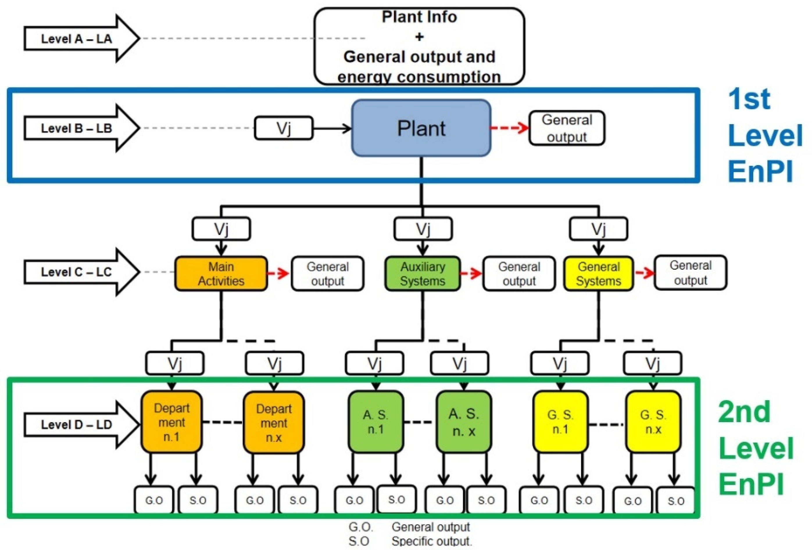
In order to describe how incoming energy carriers are used by a company, ENEA created a generic representation based on energy-flow distribution in the different company areas (namely, the “Plant Energy Model” [
44]). This identifies the energetic relationship between all involved processes and the final product. The algorithm provides numerical values representing the EnPIs of the site and of processes that take place within.
Two types of energy performance indicators are obtained:
First-level index (covering all energy carriers: electricity, thermal energy, natural gas) as:
- ○
ratio of overall final energy consumption to the amount of service provided;
- ○
ratio of per-carrier energy consumption to the amount of service provided;
Second-level index (covering the prevalent carrier(s));
- ○
specific consumption in the individual production department;
- ○
consumption by energy destination (core activities, auxiliary services, or general services)
- ○
consumption of characteristic technologies.
Underlined in
Figure 2 is the definition of first- and secnd-level EnPIs and their representation on the site energy model. The first-Level EnPIs are computed for all manufacturing four-level NACE sectors at global plant level, including all activities and processes within the site. The second-level EnPIs are obtained only for specific energy-intensive sub-sectors (i.e., cement). These indicators are calculated for specific processes of the production cycle and for auxiliary (i.e., cogeneration or compressed-air units) and general activities (i.e., lighting, HVAC, etc.).
In this way, the following indicators are obtained:
Global EnPI: includes all energy consumption;
Electric EnPI: includes only the electrical consumption of production processes (taken from power-grid and/or autonomous production, fossil fuels, renewable sources, and cogeneration);
Thermal EnPI: includes only the thermal consumption of production processes (from natural gas, heat, cold, biomass, fuel oil, coke, and other carriers);
Natural Gas EnPI: includes natural-gas consumption of processing activities.
Thermal EnPIs omit both automotive consumption (diesel, petrol, and LPG) and fuel consumption in cogeneration plants. Natural Gas EnPIs are part of the exploitation of previous thermal energy, omitting natural gas consumption in cogeneration or trigeneration. As mentioned above, the methodology used for calculating EnPIs allows for the measurement of energy consumption per given production.
2.3. Statistical Modelling for Energy Performance Indexes Evaluation
Starting from data stored in the Audit102 web portal, a definition of EnPI at the sectoral was carried out. The methodology used during this analysis can be outlined in the following steps:
2.3.1. Step 1—Selection of the Sample and Data Cleaning
The work in this phase consists of:
Qualitative and quantitative analysis of the energy consumption of every site, belonging to every four-digit NACE group stored in the ENEA database, which is the reference population.
Selection of a statistic sample from the reference population, with the aim of implementing the mathematical model.
With this aim, both energy-audit reports and summary spreadsheets containing the energy-consumption summaries are studied. A work of normalization was done in order to correct (whenever possible) or dismiss nonhomogeneous elements, such as:
audits where production is measured in different units with respect to the population;
audits lacking key information (such as the number of production units);
audits having undergone upload issues on the Audit102 portal;
audits referring to sites that, in terms of processes, do not actually belong to the considered NACE group;
sites that are clearly far from the mean trend of the energy consumption vs. production ratio (outliers).
Moreover, a numeric threshold of sites was set, conventionally equal to 5, below which the modelling was not carried out because the sample would not be statistically representative. This value can be considered conservative according to results presented in
Section 3, where statistically significant EnPIs are usually obtained with samples over 10 sites. This threshold increases the accuracy of the results with an increase in the required time for the analysis. During the first phase, some NACE groups are also separated, depending on the characteristic processes or products of the sites, or grouped in smaller intervals of production units, with the aim of obtaining a better description of the population. Finally, whenever a site is spotted whose assignment, in terms of NACE group, is clearly wrong, that site (and its audit report) is assigned to the right group.
This first normalization phase is a very time-consuming process since it requires a one-by-one audit analysis by highly specialized personnel.
2.3.2. Step 2—Calculation of the Real Sectoral EnPI (Mean +/− Standard Deviation)
For each NACE group, whenever possible, a single EnPI (EnPIr) referring to the entire group and the whole production range was calculated, or as many EnPIs as the number of partitions the NACE group has been split into. The standard deviation for EnPIr is also calculated: this is used to determine the variation range of the EnPI. In other words, from the statistics standpoint, the dispersion of the points was assessed, with respect to a positional index, or standard deviation of the observed points referring to the sample arithmetic mean. Once the mean EnPI and its standard deviation are calculated, the coefficient of variation (CV, or relative standard deviation, RSD) of the EnPI (for a given production range) is also computed as the ratio between the standard deviation and the mean value. We will define “reliability index” of the real EnPI, as a function of the CV values, as follows:
«high» if it is less than 20%
«medium» if it is between 20% and 60%;
«low» if it is between 60% and 100%;
«invalid» if it is equal to or greater than 100%
This indicator provides quantitative information about the mean value and variability of the EnPI. These values, however, should be used with caution. The use of the mean value does not include an indication of economy of scale in the production. Hence, this indicator provides valuable information about the standardisation potential of the EnPI for specific sectors. On the one hand, a high reliability is related to stable EnPIs with production and homogenous products and processes. On the other hand, a low value of the “reliability” of real EnPIs indicates a high variability of products and processes.
2.3.3. Step 3—Analysis of Linear Correlation between Consumption and Production
Regression analysis is a statistical technique that estimates the dependence of a variable (namely, energy consumption) as a function of one or more independent variables (e.g., production quantity, degree days, etc.) while highlighting the influence of several parameters. Linear regression models are used in specific measurement and verification campaigns to estimate energy savings of energy-efficiency projects and programs [
45]. In this work, we use linear regression involving two variables: energy consumption (global, electrical, thermal, or natural gas as a function of the EnPI) and production (in its specific P.U.).
Linear regression models are also preferred for analysing savings achieved with energy performance improvement actions (EPIA) in organizations with certified energy management systems (specifically between ISO 50001 and the SEP M&V protocol) [
46,
47]. The ISO 50006 standard “Energy management systems—Measuring energy performance using energy baselines (EnB) and energy performance indicators (EnPI)—General principles and guidance” recommends the use of linear regression for the estimation of indicators [
25].
For the above reasons, linear regression models are widely used for benchmarking analysis and energy-efficiency measures [
15,
26,
28,
29]. In fact, linear models are simple to develop, can be used both at the sectoral level and at the site level, and can be derived from the data provided in energy audits without any additional hypotheses.
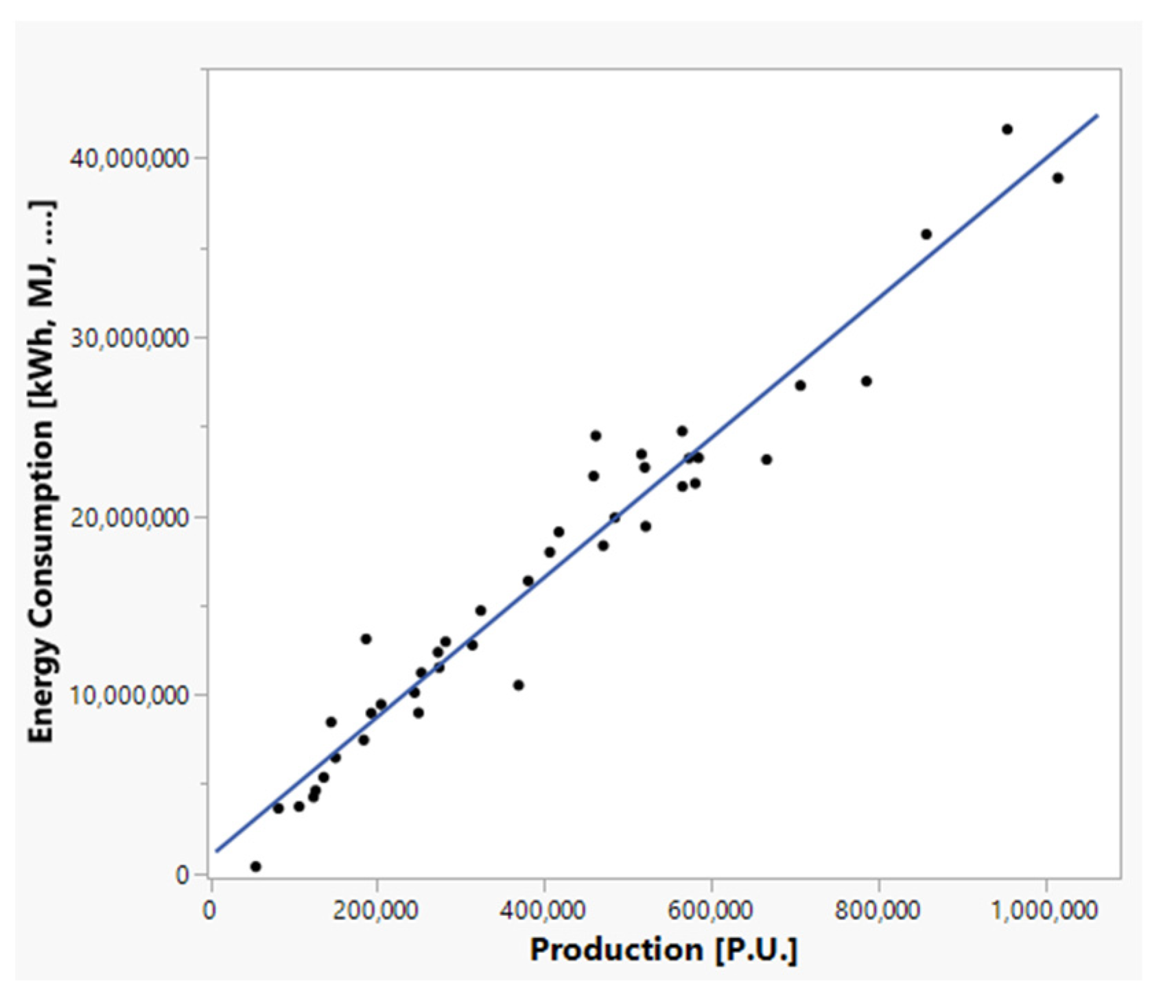
Linear regression is represented by the equation (see
Figure 3)
where
represents the final energy consumption [MJ] as the sum of a constant term,
[MJ], not dependent on the quantity of production,
, and of a variable term,
[MJ/P.U], proportional to the amount of production,
[P.U.]:
In order to evaluate the statistical representativeness of the linear correlation, the following parameters were used: R2, coefficient of determination; R, coefficient of correlation (the latter to be compared with the critical Pearson correlation coefficient (Rcrit)), and finally, the p value parameter. It is also necessary to define the confidence interval (CI) that may be achieved with the analysis. The statistical significance represents the range within which this value can deviate. In the context of this work, regarding the choice of the confidence intervals, it is necessary to establish the analytical acceptability of the model. The statistical significance defined for this model is confirmed when the maximum value for α is 0.05; therefore, the selected confidence interval (CI = 1 − α) is 95%.
In literature, R
2 is used extensively in many fields as an indicator of the strength of the correlation. Linear correlation can be considered strong if R
2 > 0.5 and moderate if R
2 > 0.25 [
48]. The strength of the correlation depends on the absolute value of R. The minimum value of R, which confirms the existence of a correlation between the variables, depends on the size of the population analysed, on α, and on the hypothesis concerning mono or bidirectionality. A significant correlation is considered to exist if R is greater than R
critic = f (N, α) [
49].
In the end, the p-value, also called the probability value, is used to confirm the representativeness of the chosen sample. If the p-Value < α, the test is considered statistically significant (confirmation of representativeness).
Hence, the correlation is considered statistically representative if
When the model did not show a significant linear relationship between energy consumption and production, the mere EnPIr calculated for every NACE group and its standard deviation were used to describe the sectors.
The analysis of these three correlation variables is only the first step. A low value certainly indicates an insignificant relationship between consumption and production (often due to the presence of economic factors). Meanwhile, a high value of the coefficient may not guarantee a significant relationship. The correlation coefficient can be very sensitive to “outliers” and may indicate association when, in fact, none exists. It is important to note that one or few anomalous items can have a large impact on R. Hence, it is necessary to inspect a plot of the data and to ensure that the data covers the range uniformly.
2.3.4. Step 4—Formulation of Specific EnPI Model (EnPIm)
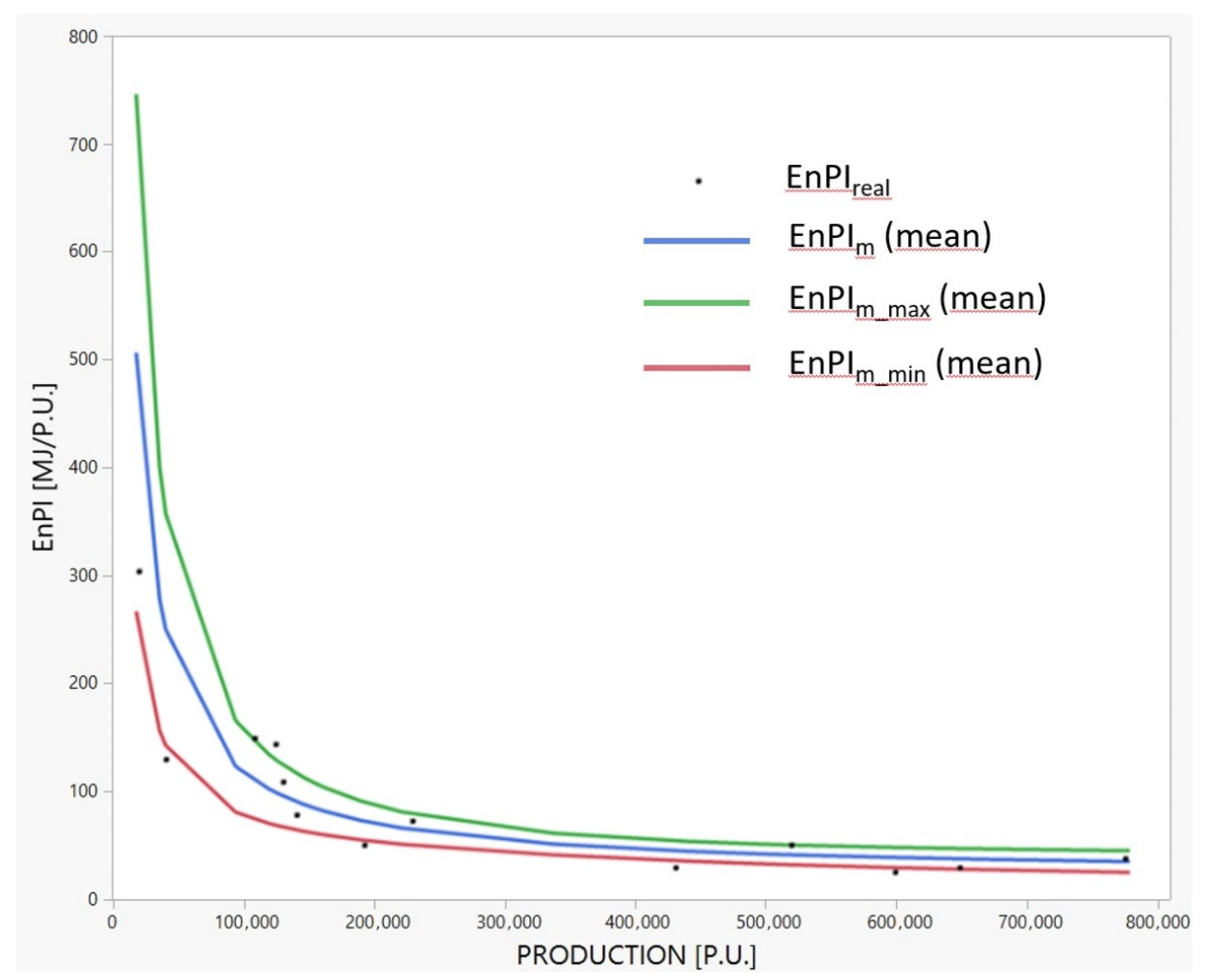
As previously explained, a generic EnPI is calculated as the ratio of energy used for producing a unit of product (P.U.). Hence, following the statistical analysis of linear regression, EnPI
m is calculated dividing both sides of the production function and is represented by a hyperbolic function:
where
and
, respectively, represent the slope and the intercept of the linear regression line.
With this approach, it is possible to represent the analytical model of EnPI (in blue in
Figure 4), and the specific EnPI by site can be subsequently compared with the sectoral main value.
An analysis of uncertainty of the EnPI
m has been developed to a defined significance level (α = 0.05). The uncertainty analysis is based, in a general way, according to the central limit theorem, which, in a very simplified way, allows for the assumption that the EnPI
m presents a Gaussian dispersion. Therefore, it is possible to define an upper- and lower-limit curve of statistical significance of the formula model.
The uncertainty σ of the EnPI
m model is calculated through the propagation of the statistical error, which is obtained on the basis of the covariance matrix, C
i,k, as follows:
where
refers to the EnPI
m function and x
i e x
k are the parameters a and b estimated in the regression model. Substituting in the estimated consumption, the formula for the propagation of the statistical error becomes
Figure 4 shows the mean theoretical curve (in red) of the EnPI
m and its lower (red) and upper (green) limits at 2σ. Moreover, the real EnPI values of the individual sites analysed are also presented (black dots).
This graph allows for easy visualization of the effects of error propagation in the calculation of the EnPIm as a function of the production. The area contained between EnPIm _max and EnPIm _min represents the “variability” of the statistical case.
In practice, the confidence interval derived from the previous equations is displayed, associated with the linear regression built based on the consumption vs. production, which represents the uncertainty of the EnPI
m, graphically delimited by the lower and upper limit of the curve. In this way, for each diagnosis analysed, it is also possible to evaluate the value of the real EnPI with respect to the theoretical interval thus defined and to quantify the error that affected it. This model can be used as the basis for more advanced models, such as stochastic frontier analysis (SFA) [
31], index decomposition analysis (IDA) [
50], or data envelopment analysis (DEA) [
51] for calculation of energy-efficiency impact or deviation from benchmark.
The statistical method developed and illustrated in the previous sections was applied using energy data included in the energy audits uploaded to the Audit 102 web portal at the end of December 2019.
Compared to the methodologies present in the literature [
16,
18,
19], the methodology developed in this work has a different approach. In fact, starting from the available data set (the mandatory energy audits pursuant to art.8 directive 27/2012), we tried to find a correlation between energy consumption and production rate, assigning a level to the data set, the reliability of which is linked to the difference between the average and the standard value. The main advantage lies in its replicability in all production sectors, both in the industry and in the tertiary domains.
3. General Results of NACE 23 Division
The previously illustrated methodology was applied to more than 300 four-level NACE sectors. The quality of statistical modelling of the EnPIs is strongly dependent on each sector analysed. Specifically, it depends on the sample dimension, on the heterogeneity in terms on production range and units adopted, on the structure of energy uses, and on energy intensity of the production.
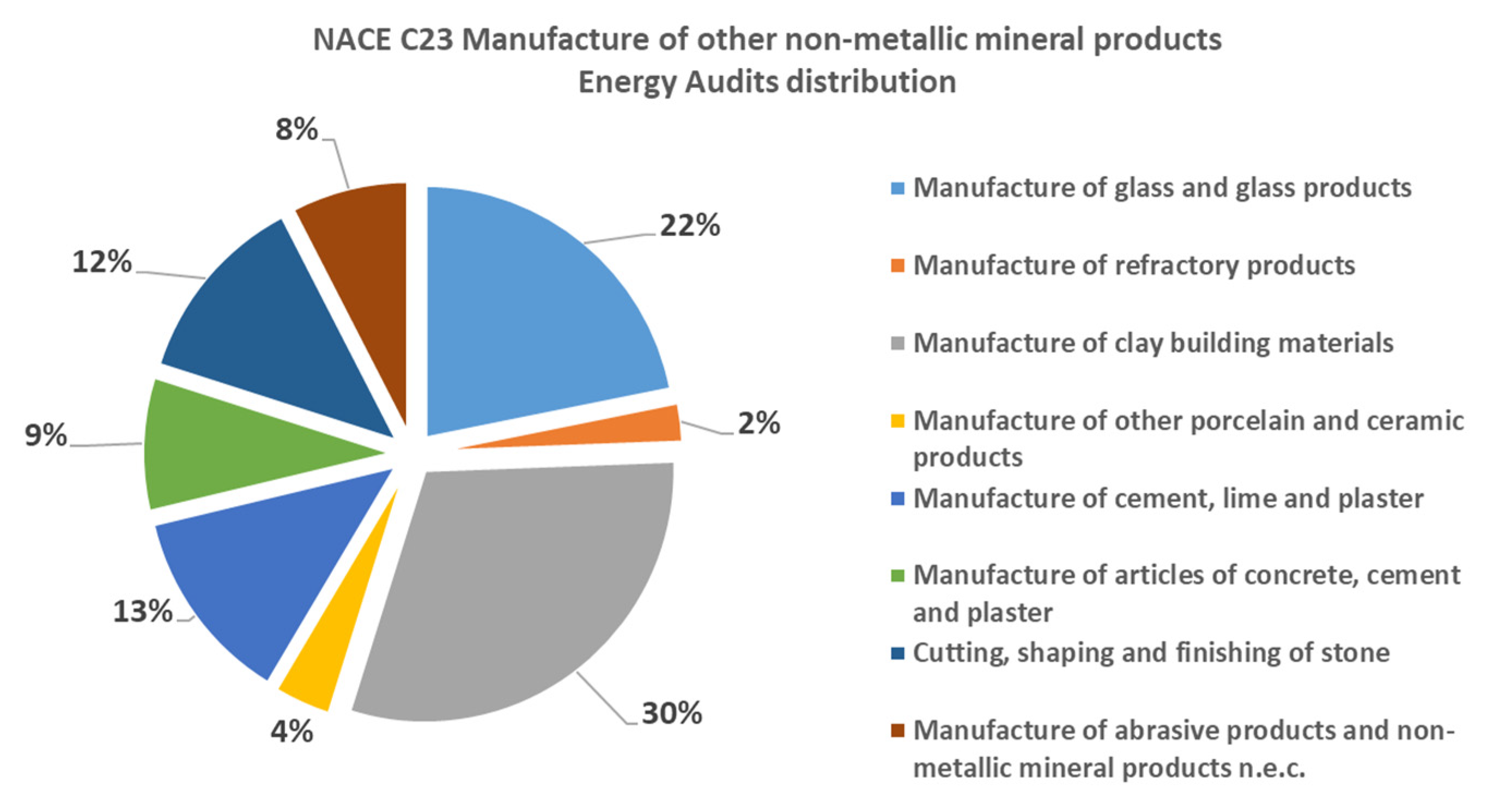
Hence, on the one hand, there are sectors with high reliability and quality of EnPI model (e.g., cement, refineries, foundries, ceramics). On the other hand, some sectors provide EnPIs with little significance (e.g., machinery manufacturing, electronics, furniture, or mining and quarrying). This section shows, as an example, the results obtained from the analysis of the NACE 23 division, “Manufacture of other non-metallic mineral products”. The NACE 23 division includes 512 energy audits distributed among the different groups, as shown in
Figure 5. The final global energy consumption of the NACE 23 EAs amounts to about 2.6 × 10
5 TJ (corresponding to about 13% of the global energy consumption of audited sites).
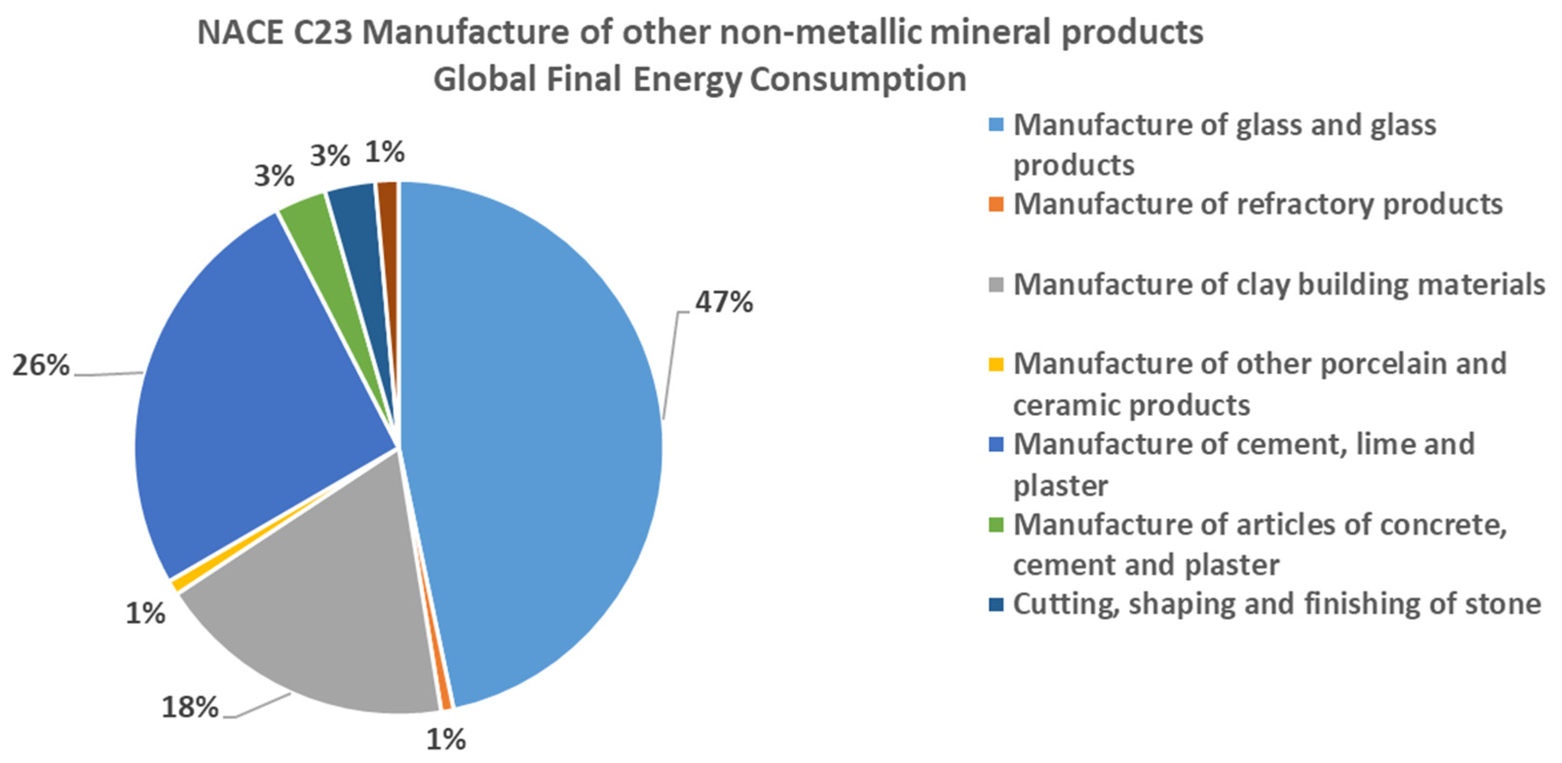
The distribution of audited sites’ final energy consumption among the various NACE 23 groups is reported in
Figure 6, which shows that consumption is mainly attributable to glass manufacturing (47% of the total), followed by the cement industry (26%) and the manufacture of clay building materials (18%).
The NACE 23 division, in its Italian transposition (ATECO), includes 29 six-digit subcodes, and the analysis presented in the previous sections was set up for each of them. Real IPEs (see
Section 2.3, Step 1) and model IPEs (see
Section 2.3, Step 4) were calculated for six-digit subcodes where the number of diagnoses and the consistency of the data contained in them in terms of volumes, production processes, and units of production rates allowed it.
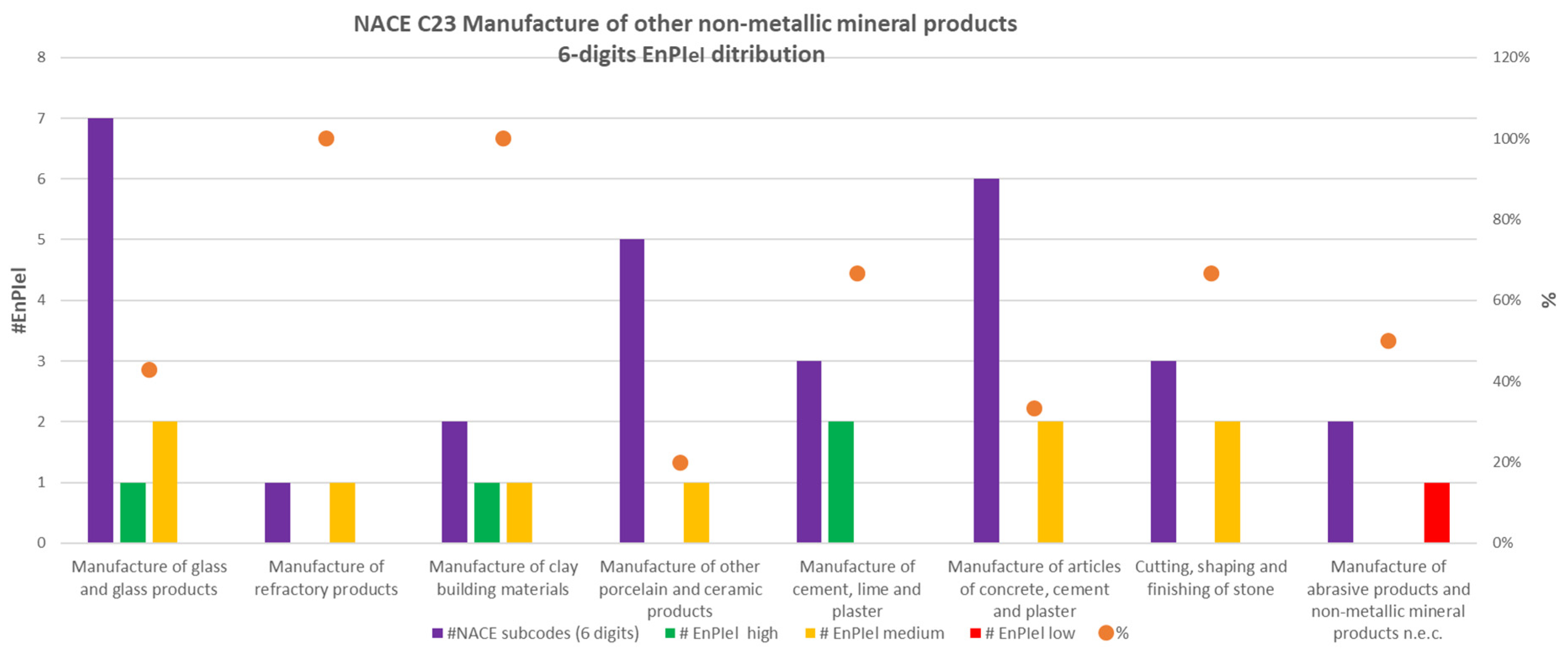
A total number of 41 actual EnPIs were calculated, of which 32% had high reliability, 61% had medium reliability, and the remaining 7% had poor reliability. Of these 41 EnPIs, 14 are electrical, 2 thermal, and 15 global.
Figure 7 shows, as an example, the distribution of electrical EnPIs by NACE subcode. The different colours indicate the reliability of the indexes identified. For some sub-codes, there is a higher percentage and better reliability of the identified indexes (e.g., for cement), while for others, few EnPIs have been identified and with a low reliability, mainly because of sample dimension. As shown in
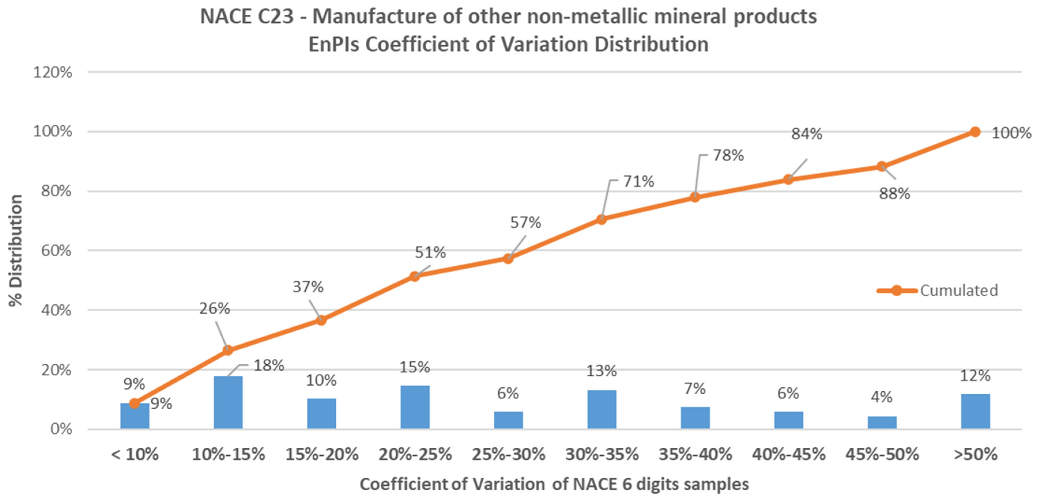
Figure 8, the range of the coefficient of variation for the greatest number of six-digit EnPIs (about 18%) is 10–15%. Globally, some 25% of NACE 23 four-digit EnPIs have a coefficient of variation lower than 15%, and about 50% lower than 25%.
In addition to the elaboration of actual EnPIs, the linear correlation between consumption and production for NACE 23 four-digit subcodes was evaluated to develop specific ENPI models.
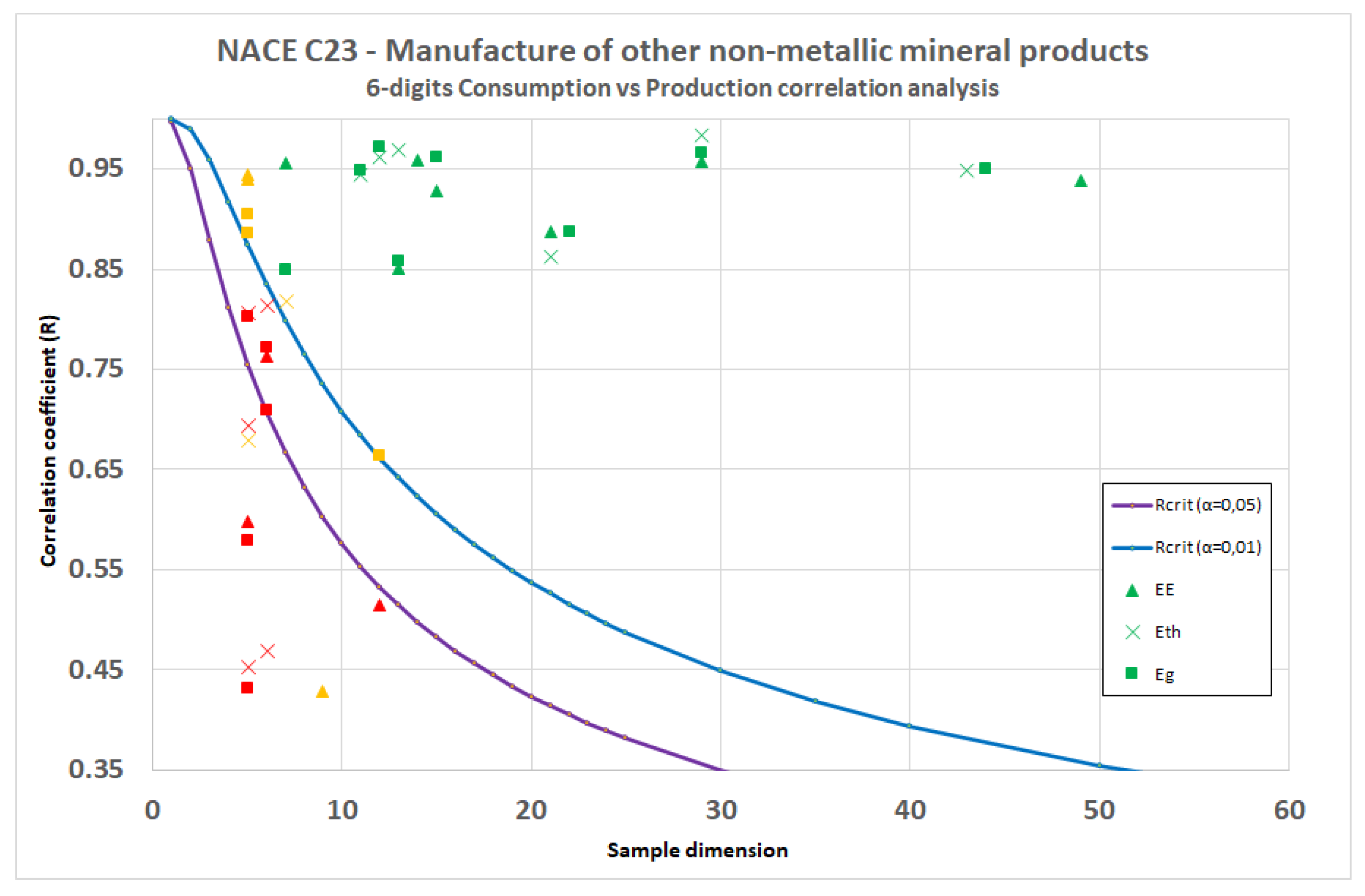
The main results of the correlation analysis are summarised in
Figure 9. The two curves (in purple and blue) represent critical values of the Pearson correlation coefficient (R
crit) as a function of sample dimension for a confidence value α of 0.05 and 0.01. The indicators (triangles for electrical energy consumption, crosses for thermal energy consumption, and squares for global energy consumption) represent the correlation coefficient values (R) of the linear regressions for the different ATECO six-digit subcode sets. As explained in the dedicated paragraph, in order to regard the correlation as statistically representative, it is necessary to evaluate not only that R > R
critic = f (N, α) but also that the P-value is sufficiently low. In the figure, the indicators have been coloured according to the
p value of the linear regression. In red are the indicators for which
p value > 0.05; in orange, those for which 0.05 <
p value < 0.01; and in green, the correlations with
p value < 0.01.
As can be seen from
Figure 9, the sample dimension has a substantial impact on the statistical significance of the correlation. The minimum sample size to be considered for the case study is approximately 8/10 EAs.
4. A Case Study: The Cement Industry
An additional focus on the cement industry (NACE 23.51) is presented in this section, as part of NACE 23 sector “Manufacture of other non-metallic mineral products”. In this detailed analysis, the methodology was applied to the development of first- and second-level EnPIs. The normalization work that was pre-emptively accomplished in order to correct or dismiss nonhomogeneous elements: a partition of NACE group 23.51 depending on the characteristic processes of the sites.
In the cement sector, 47 energy audits were collected by ENEA in December 2019, in compliance with Article 8 of Italian Legislative Decree 102/2014:
1 energy audit related to an administrative site;
14 energy audits related to sites where only the grey-clinker-grinding phase is carried out;
30 energy audits related to sites where the complete grey-cement production cycle is carried out (in one of these sites, white cement was also produced;
2 energy audits related to sites where the complete white-cement production cycle is carried out.
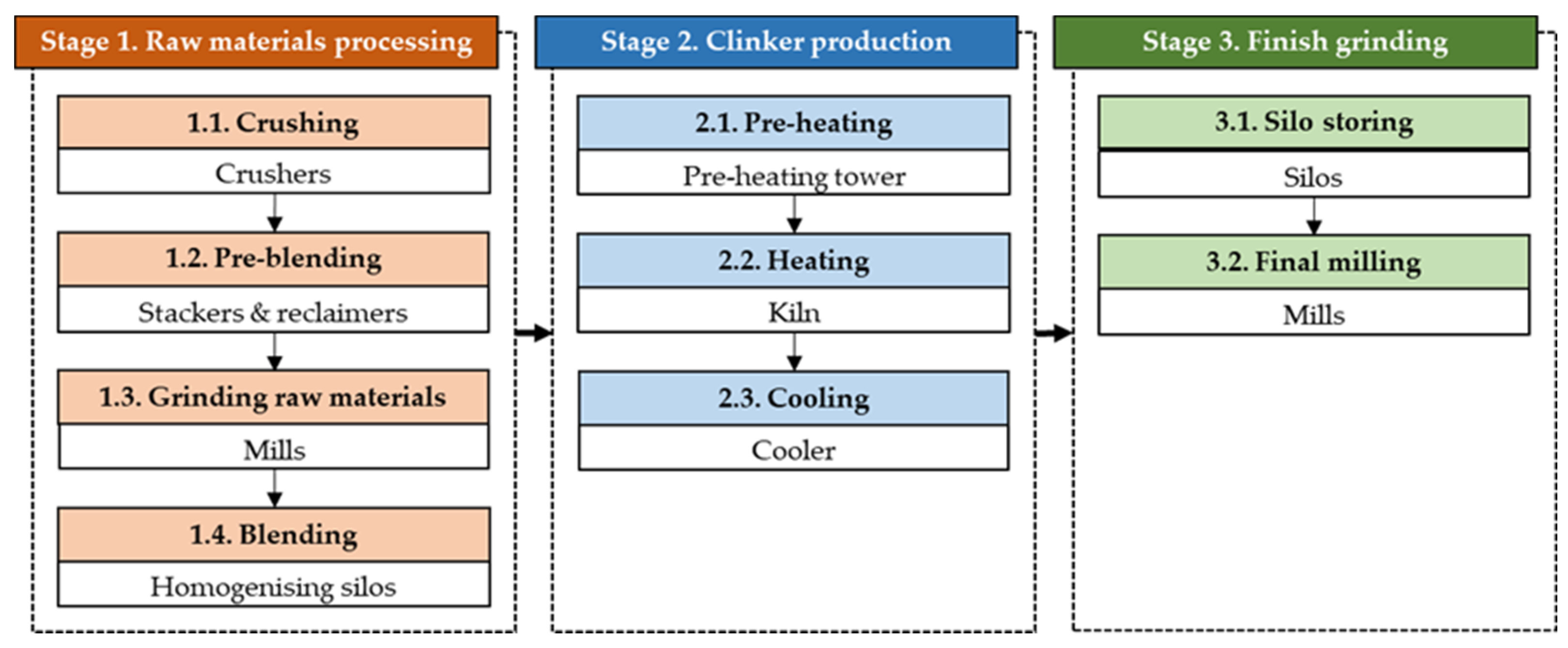
Consumption data, gathered from 29 out of 30 energy audits related to the complete grey-cement production cycle (one site was dismissed because of non-continuous production), were subjected to the developed statistical method, with the purpose of assessing energy performance indicators of the Italian cement industry sector. The diagram in
Figure 10 represents the complete grey-cement production cycle.
4.1. Energy Consumptions in Complete Grey-Cement Production Cycle
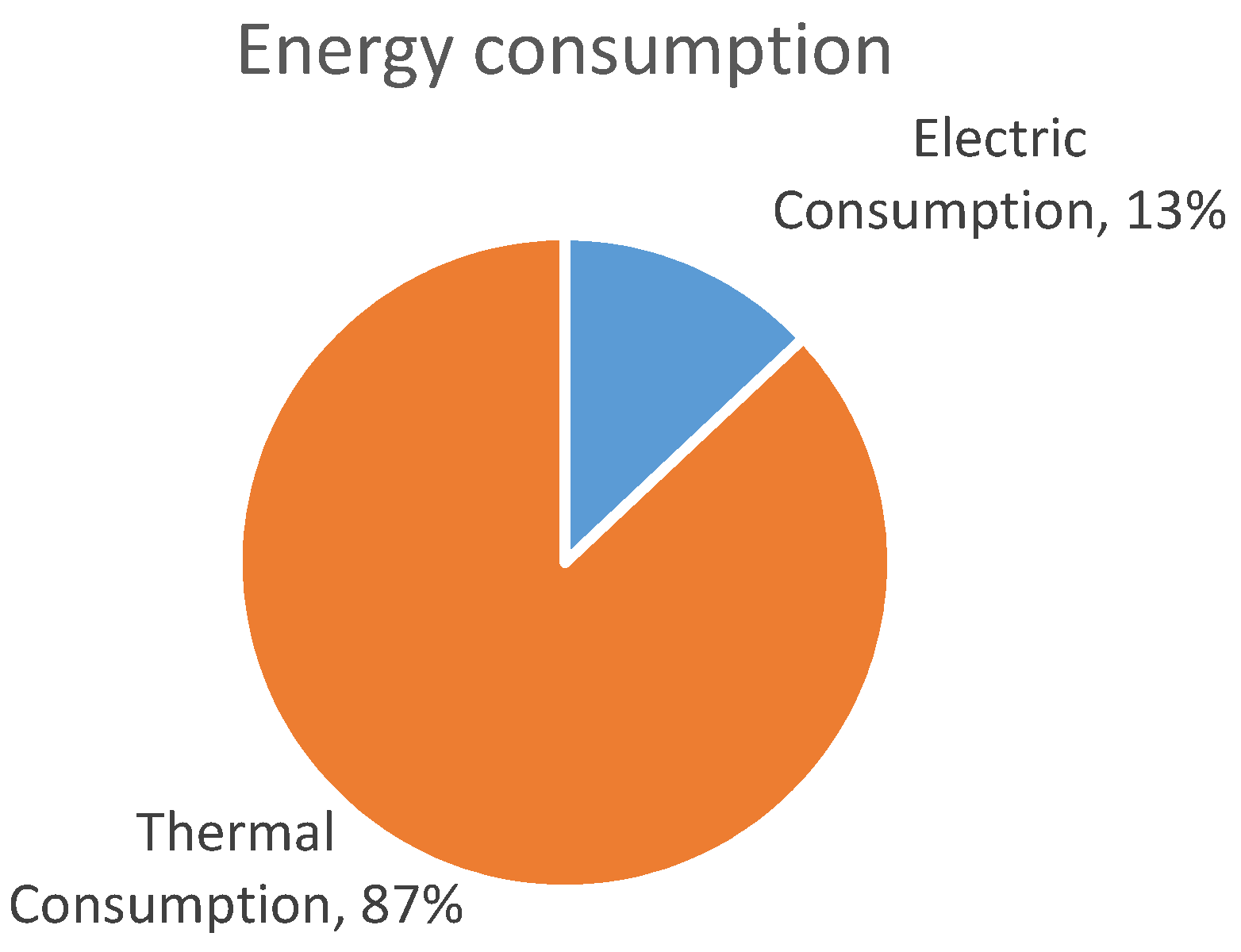
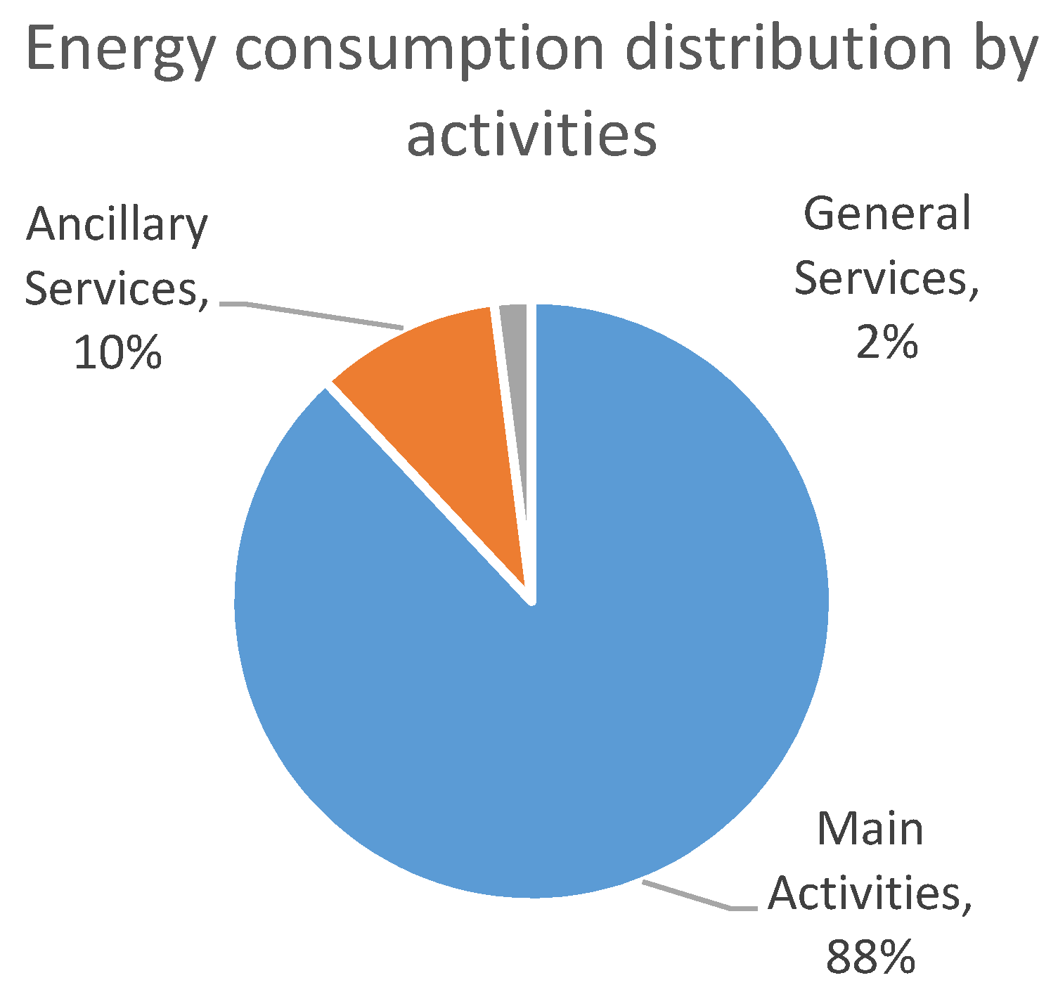
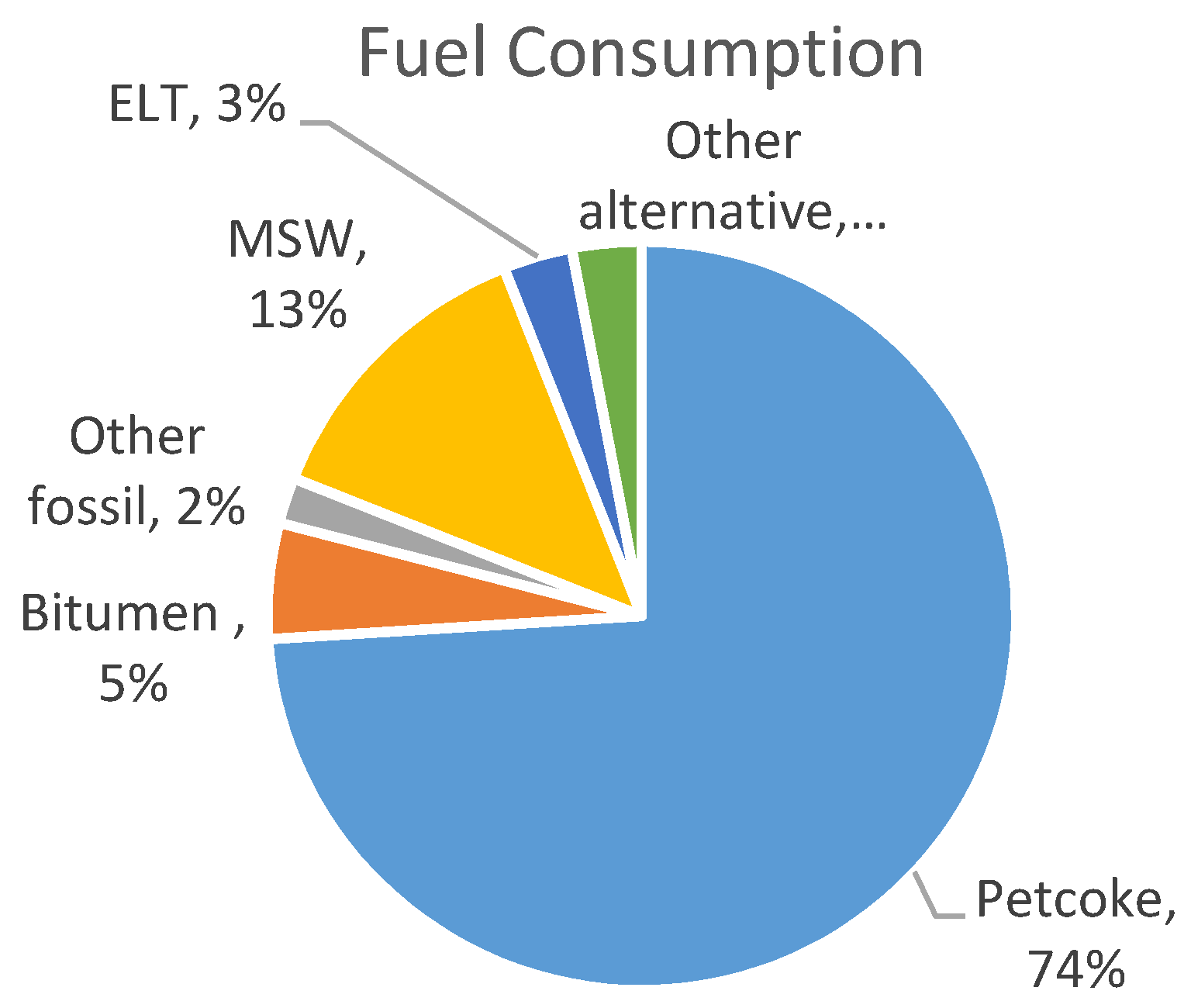
Figure 11 shows the global energy consumption distribution between electricity and heat for the grey-cement production cycle, while
Figure 12 shows the global energy consumption distribution by activities (main activities, auxiliary services, and general services).
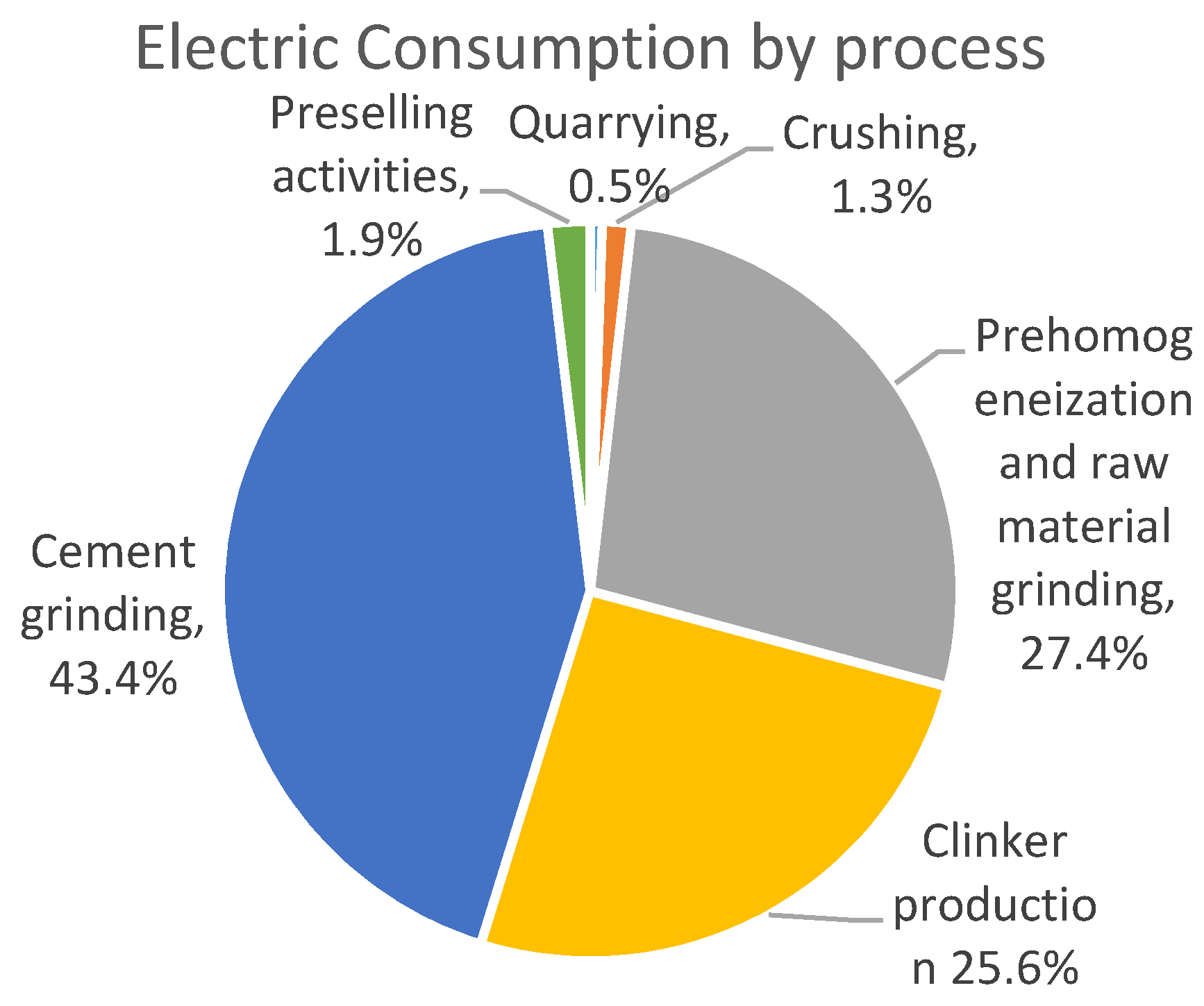
Figure 13 shows the distribution of thermal consumption by fuel, while
Figure 14 shows the distribution of electric consumption by activities.
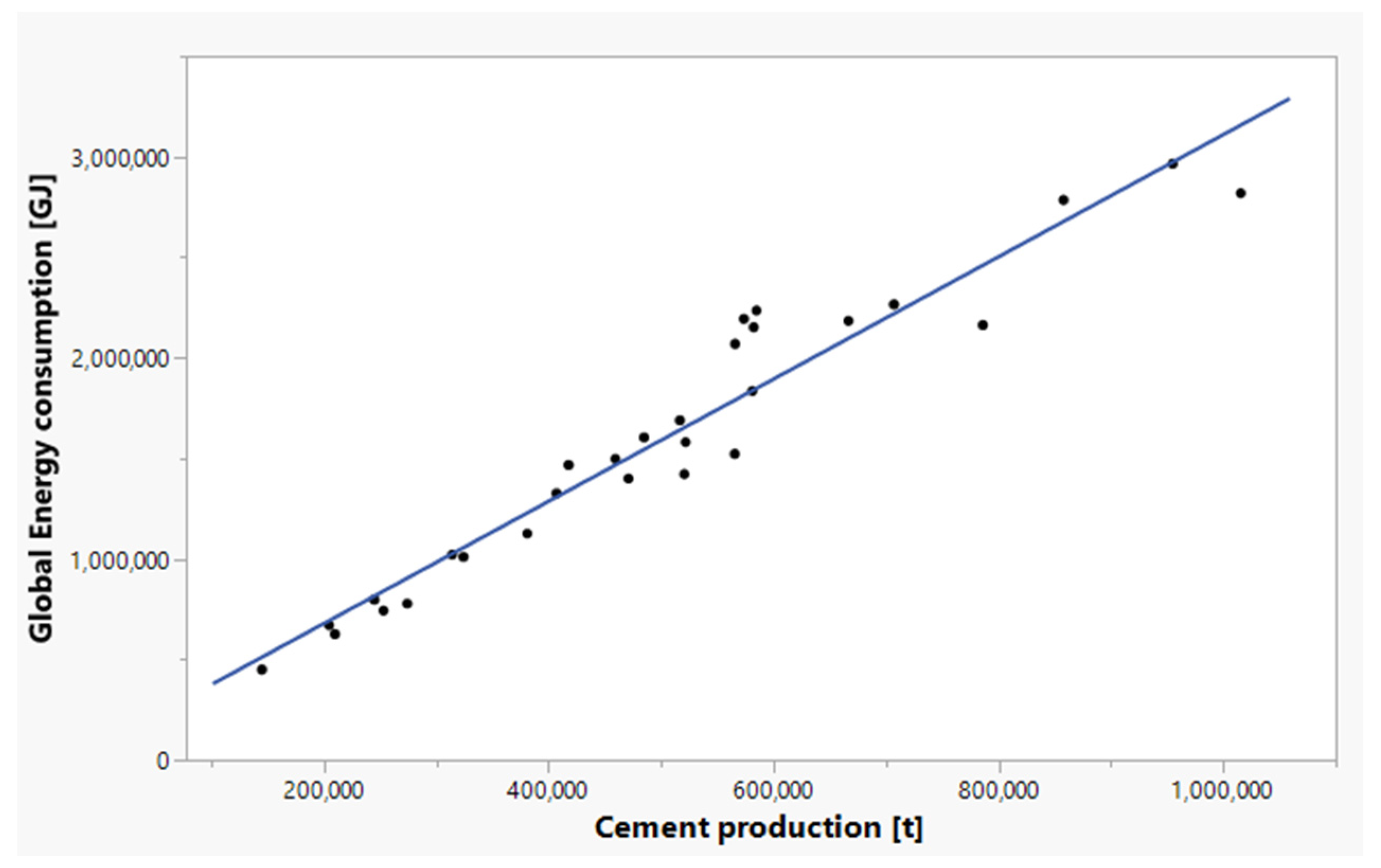
4.2. Electric, Thermal, and Global Energy Consumption
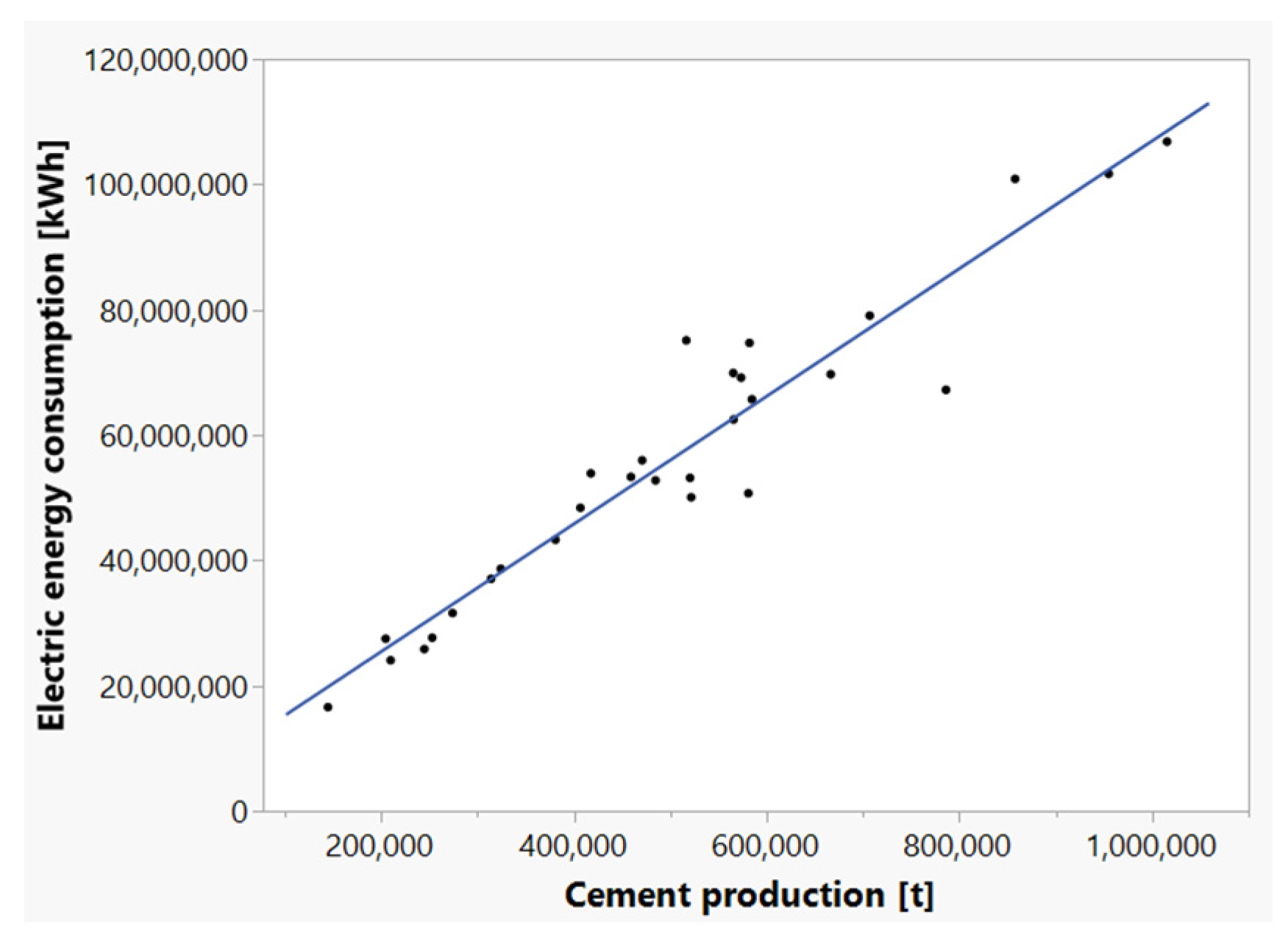
First, data of electric, thermal, and global consumption of each site, including those relating to auxiliary services and general services, were processed. In line with the proposed methodology, two EnPIs referring to two production ranges were calculated, and the linear regression between energy consumption (electric, thermal, and global) and production (in its specific P.U.) was analysed. Electric consumption was compared with the actual cement produced on site, expressed in tons. In order to take into account the fact that many cement production sites sell or buy clinker, take it from stocks, or put it in stock, a “virtual” electric consumption related to the complete production cycle of all cement actually produced on the site was calculated. Electric consumptions related to the quarry phase and the raw materials in the grinding phase (if carried out on site) were excluded, as these phases are not always present in the sites.
Electric consumption of clinker during shipping (where applicable) was also excluded, with the purpose of considering only electric consumption of the complete grey-cement production cycle.
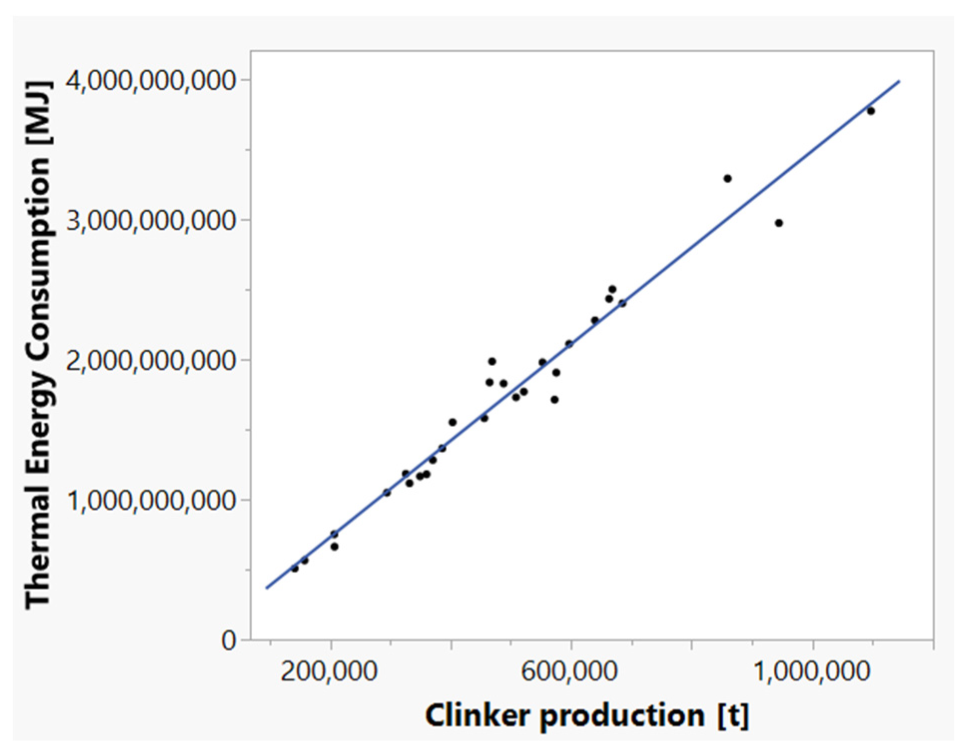
Thermal consumption refers to clinker quantity produced on site (in tons) and to a “virtual” cement production calculated from the ratio between the clinker actually produced on site and the R parameter (ratio between the amount of clinker ground on site and the amount of cement actually produced). Consumption of diesel and LPG fuel, mainly used for transport (both normal vehicles and quarry vehicles, if any), was excluded from thermal consumption.
Global consumption refers to the amount of cement produced on site, expressed in tons. Additionally, for global consumption, as for electric consumption, in order to take into account the fact that many cement plants sell or buy clinker, take it from stocks, or put it in stock, an elaboration of global consumption was made in order to calculate, for each site, a “virtual” global consumption related to the complete production cycle of all cement actually produced on the site. In particular, as for electric components, the “virtual” electric consumption previously computed was considered, while for thermal components, a “virtual” thermal consumption was considered relating to the production of all the clinker necessary for cement actually produced on site. Global consumption included both electric consumption at the quarry stage, the raw materials in the grinding phase in the plant (if any), and thermal consumption of LPG and diesel fuel used for transport (both on ordinary and quarry vehicles, if any), while those of the clinker shipping phase were excluded.
Table 1 shows real electric, thermal (referring, respectively, to cement and clinker), and global EnPIs and their standard deviations. The table also shows that the reliability of EnPIs is high.
Linear regression models for electric, thermal (referring to clinker) and global consumptions are shown, respectively, in
Figure 15,
Figure 16 and
Figure 17, while
Table 2 shows statistical regression parameters: linear regression equation, coefficient of determination (R
2), Pearson correlation coefficient (R),
p value, size of the population analysed (N), and Rcritic for α = 0.001 e α = 0.005.
The correlations are statistically representative as
p value < 0.0001 and R > Rcritic = f (N, α); as shown in
Table 2, R2 is greater than 0.9, and the confidence value is 99% for each linear regression.
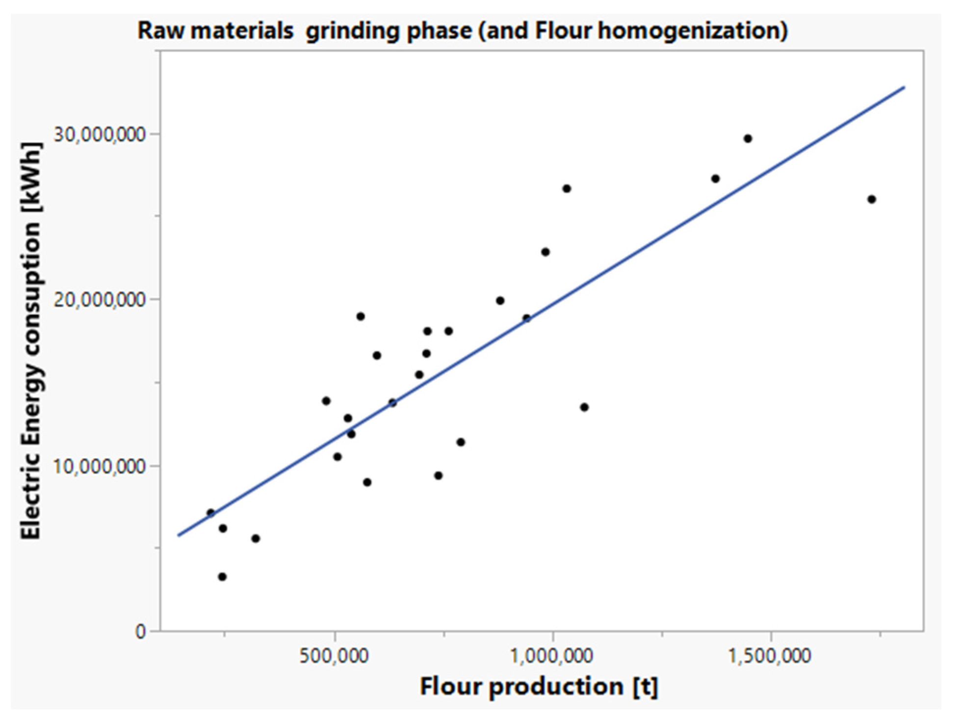
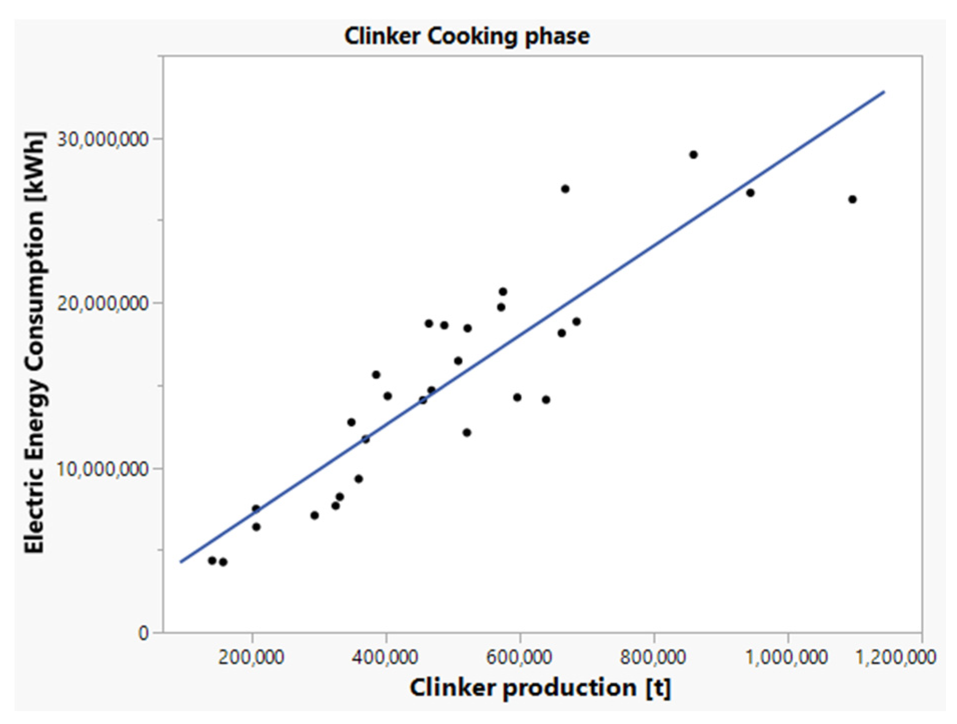
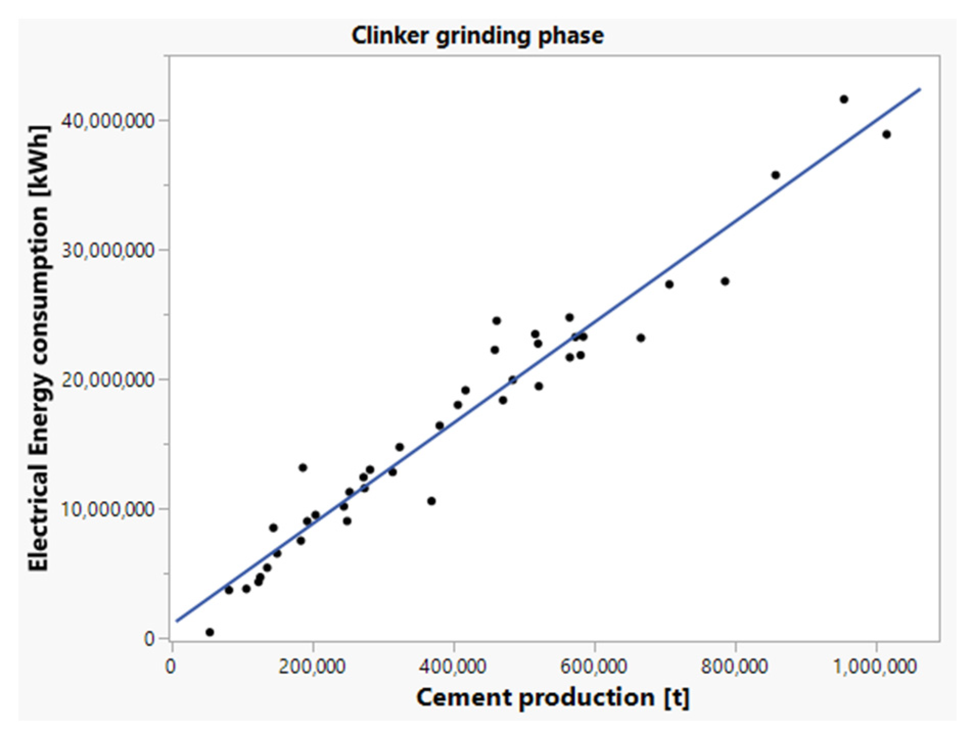
4.3. Second-Level EnPIs—Main Phases of Grey-Cement Production Cycle
The methodology was subsequently applied to sub-process levels (second-level EnPIs, as presented in
Figure 2). Hence, consumption data of main phases of the grey-cement production cycle were subjected to statistical modelling. In particular, raw materials in the grinding phase (and homogenisation of flour), the clinker grinding phase, featuring electric consumption, and the clinker cooking phase, featuring electric and thermal consumption, were considered.
Electric consumption of raw materials in the grinding phase was compared to the amount of flour actually produced on site, expressed in tons.
Electric consumption of clinker in the cooking phase was compared to the amount of clinker actually produced on site, expressed in tons.
Electric consumption of clinker in the grinding phase was compared to the amount of cement actually produced on site, expressed in tons. In this case, the sites where only the clinker grinding process is carried out were also considered in the sample.
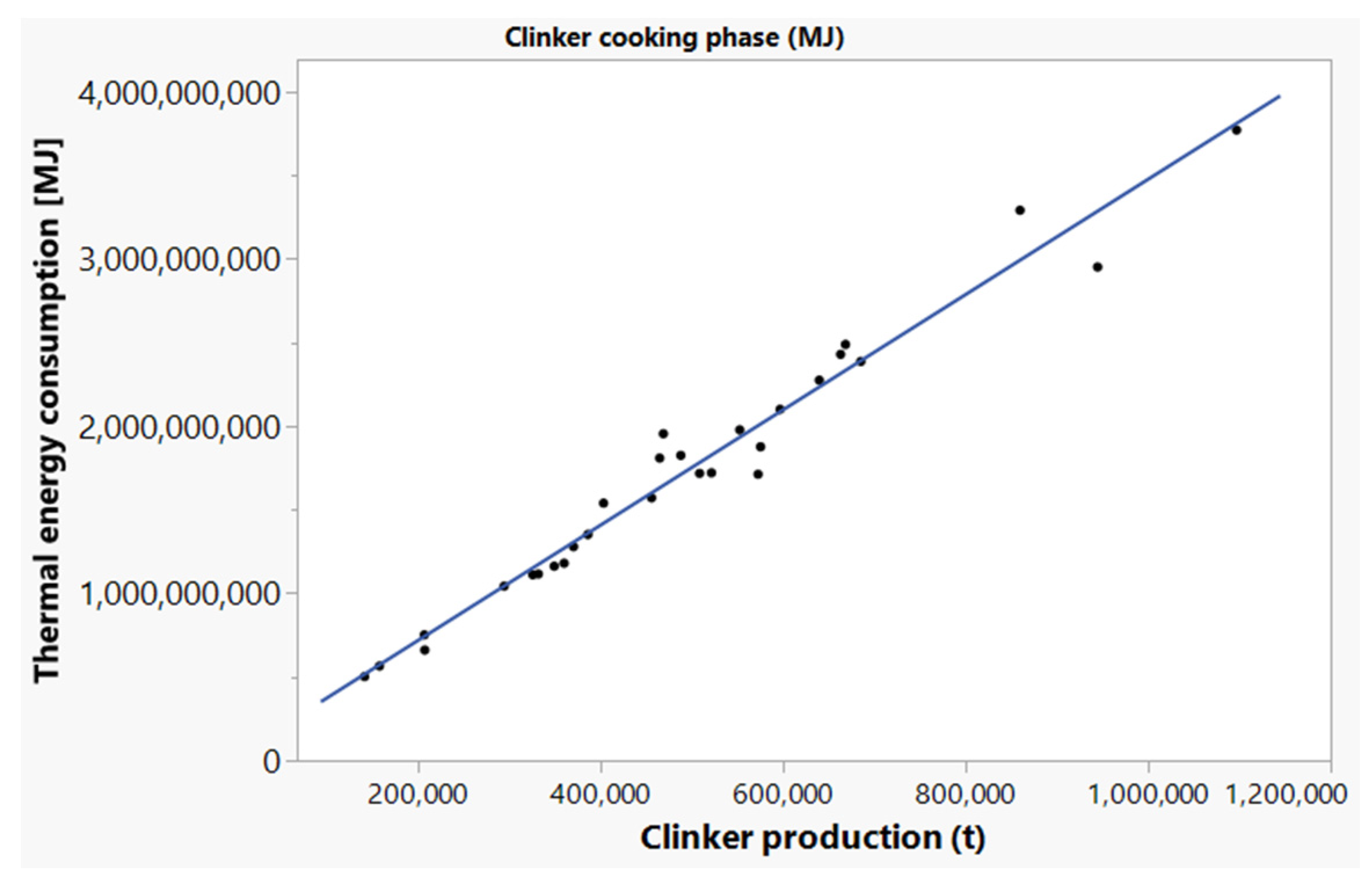
Thermal consumption of clinker in the cooking phase was compared to the amount of clinker actually produced on site, expressed in tons.
Table 3 shows real electric and thermal EnPIs for the main phases of the grey-cement production cycle and their standard deviations. The table also shows the reliability of EnPIs.
Linear regression models for electric and thermal consumptions for the main phases of the grey-cement production cycle are shown, respectively, in
Figure 18,
Figure 19,
Figure 20 and
Figure 21, while
Table 4 shows statistical regression parameters: linear regression equation, coefficient of determination (R2), Pearson correlation coefficient (R),
p-value, size of the population analysed (N), Rcritic for α = 0.001 e α = 0.005. Those correlations are statistically representative as
p-value < 0.0001 and R > Rcritic = f (N, α); as shown in
Table 2, R2 values are high, and the confidence value is 99% for each linear regression.
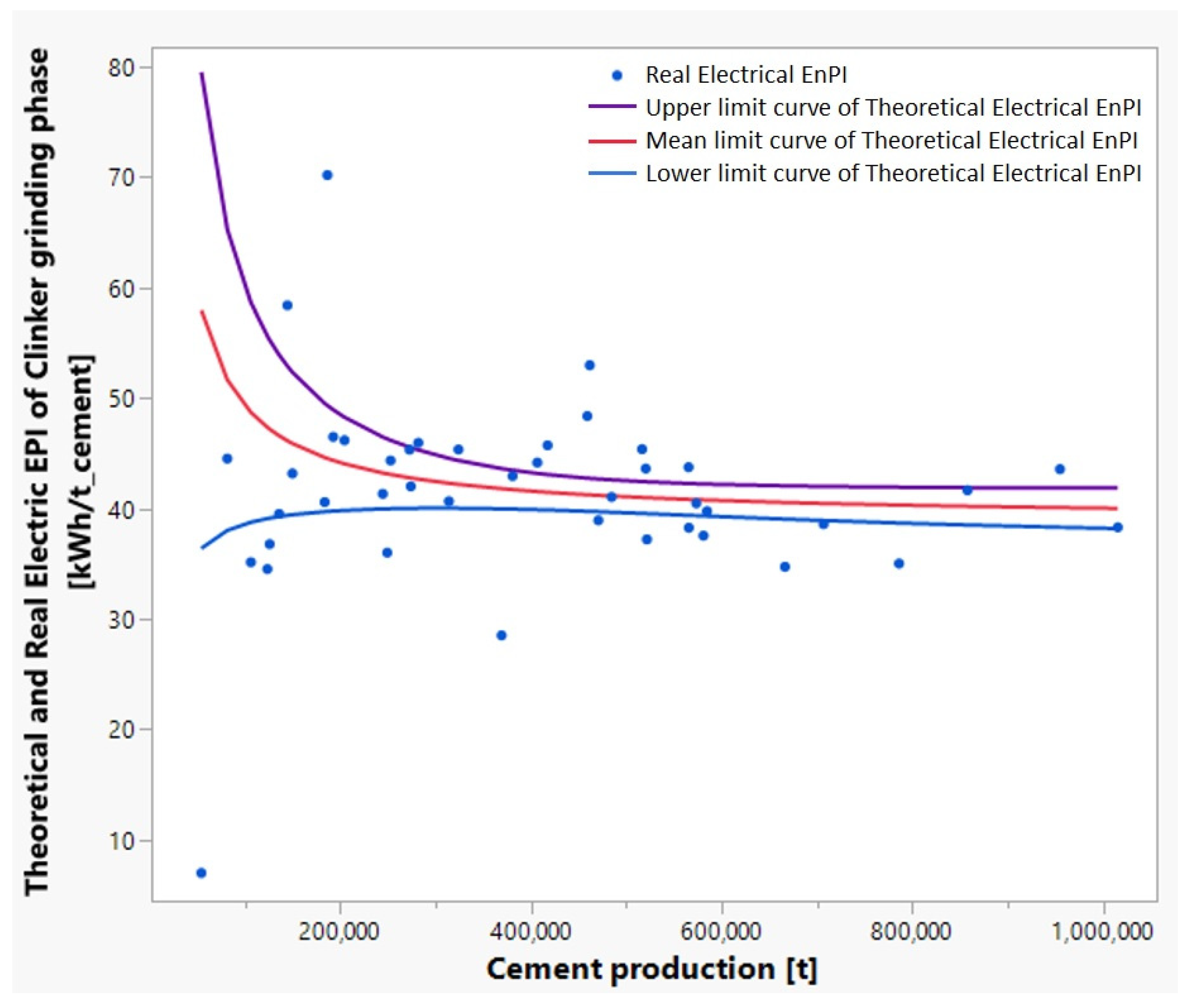
For the clinker grinding phase, the hyperbolic function of electric EnPIs was calculated, and
Figure 22 shows the theoretical (in red) curve of EnPI, its lower (blue), and upper (purple) limits at 2σ. Moreover, the real EnPI values of the individual sites analysed are also presented (blue points).
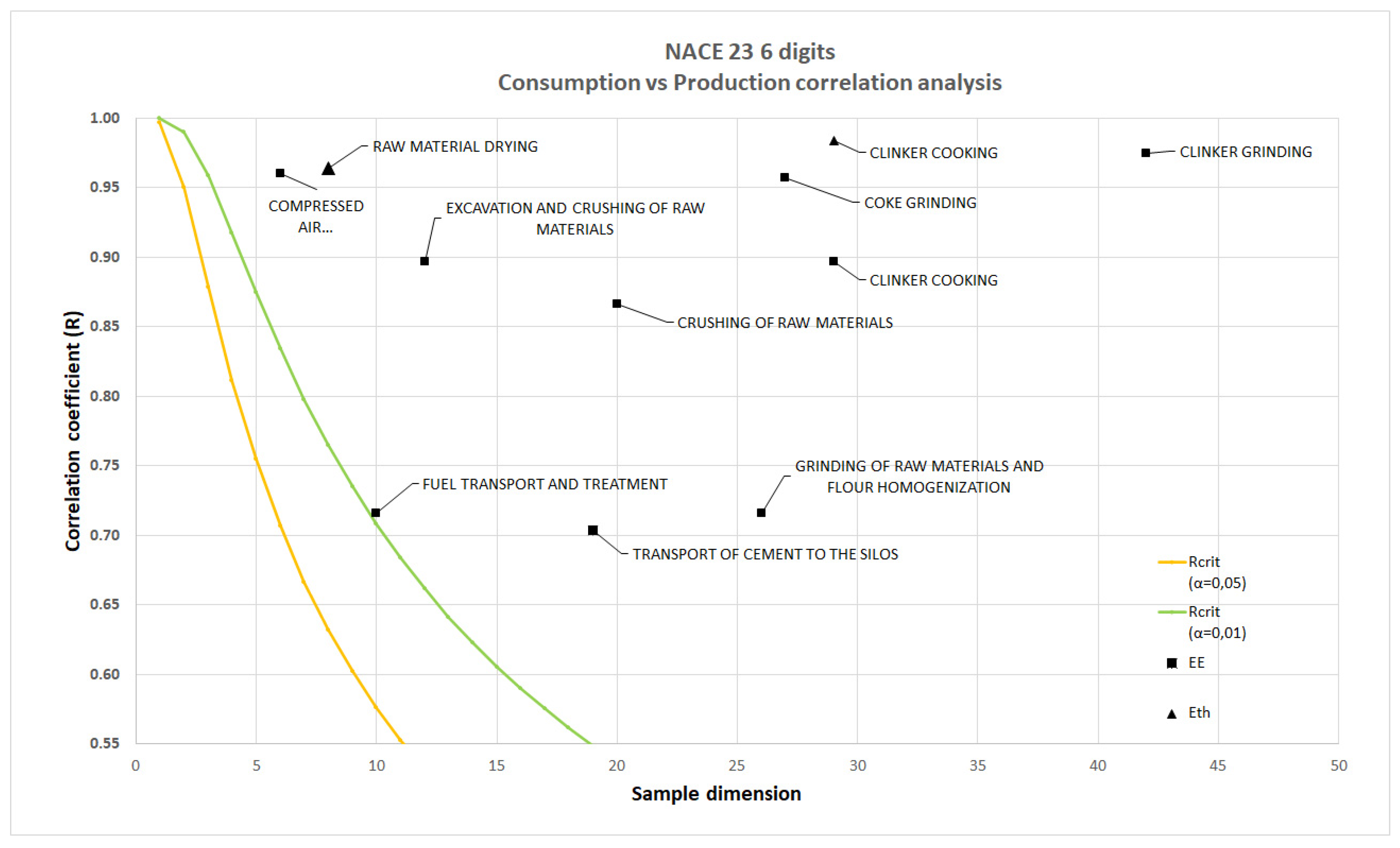
The results of the consumption vs. correlation analysis for the main production phases and auxiliary services for NACE 23.51 are summarized in
Figure 23. As can be seen from the figure, although in some cases, the sample dimension is small (lower than 10 EAs), the correlations are statistically valid, given the values assumed by the correlation coefficients, R, and considering that for all of them, the
p value is lower than 0.0001. The phases for which the electricity consumption vs. production correlation appears weaker are fuel transport and treatment, transport of cement to the silos, and grinding of raw material.
Numbers of Cyclones
Another application of the methodology involves energy consumption related to other variables of the plant design. Specifically, the impact of the number of cyclones on the pre-heating phase before clinker production was evaluated. In only 23 out of the 29 sites where the complete grey-cement production process is carried out, the number of cyclones of the furnace is provided.
In detail:
in 11 of the 23 sites, the number of cyclones is equal to 4;
in 12 of the 23 sites, the number of cyclones is equal to 5.
Table 5 shows actual thermal EnPI and its standard deviation for the entire production range in the two cases of four or five cyclones. The table also shows that the reliability of thermal EnPI for the clinker cooking phase is high in both cases.
4.4. Validation
In
Table 6, a comprehensive validation of EnPI obtained in this work with public data is provided. The data are aggregated by country or, when possible, only by dry process with multistage (three to six stages) cyclone preheaters and pre-calcining kilns.
The first level electric and thermal EnPI values is in line with the BREF sector [
52] (which reports electric and thermal EnPIs values, respectively, between 90 and 150 kWh/t_cement and between 3.000 and 4.000 MJ/t_clinker) and with IEA data [
53] (which report, for Italy, values, respectively, of 122 kWh/t_cement and of of 3.500 MJ/t_clinker), the most relevant benchmark for the sector in the EU. First-level EnPI values confirm that Italian cement presents a high overall energy efficiency—3.5 GJ/t
clinker—compared to the global range of 3.0–4.2 GJ/t
clinker. On the one hand, the lowest value corresponds to India, at 3.0 GJ/t
clinker (with different product requirements and processes), and the lowest value between OECD economies correspond to Japan, at 3.4 GJ/t
clinker. On the other hand, the mean values for the EU-28 and U.S. are 3.7 GJ/t
clinker and 3.8 GJ/t
clinker, respectively. Therefore, the Italian cement sector is very efficient in terms of energy consumption.
The information for second-level EnPIs is scarce, but the obtained electrical EnPI values for raw-material preparation, solid-fuel preparation, finish grinding, and clinker cooking are slightly higher than the best available technologies (BAT) [
54] and lower than the values for the U.S. as of 1999 [
55].
Ref. [
56] presents values of the impact of the number of preheating cyclones on clinker thermal consumption. The values obtained in this work are in line with literature data:
- -
4-cyclons preheating: 3.6 GJ/tclinker. Overall range 3.2–3.6 GJ/tclinker
- -
5-cyclons preheating: 3.4 GJ/tclinker. Overall range 3.1–3.5 GJ/tclinker
Lastly, a similar analysis of thermal energy consumption as function of the clinker production is presented in [
57]. Oda et al. analysed the impact of different technologies and modelled the SEC with a logarithmic function. The EnPI range is similar to that obtained in the present work; however, it cannot be directly compared due to a lack of statistical significance or correlation information.
Table 6.
Validation data of calculated EnPI for the cement sector.
Table 6.
Validation data of calculated EnPI for the cement sector.
| | | | This Work | EU BREF | IEA 2021 | EU 2012 | ASIA 95 | UN 2010 | EU 2019 | US 99 | World 2012 | World 2012 | EU 2012 | BAT 2005 | BAT UN 2010 |
|---|
| | | | | [52] | [53] | [58] | [59] | [22] | [60] | [55] | [61] | [57] | [58] | [54] | [22] |
| Clinker production | Global | GJ/t | 3.5 | 3.0–4.0 | 3.5 | 2.8–3.7 | 2.1–5.4 | 3.3–4.2 | | | 3.0–6.5 | 3.0–4.5 | 3.0–4.2 | 2.85 | 2.9 |
| Electrical | kWh/t | 28–32 | | | | | | | 45 | 60–100 | | | 22.5 | |
| Thermal | GJ/t | 3.4–3.6 | | | | | | | 4.6 | | | | | |
| Cement production | Global | GJ/t | 3.1–3.3 | | | | | | 2.1–5.1 | | | | | 2.71 | |
Electrical
(with griding) | kWh/t | 108–111 | 90–150 | 122 | | 93–162 | 109–134 | | 150 | | | | | 56 |
| Thermal | GJ/t | 2.8 | | | | | | | 4.2 | | | | | |
| Raw-Material Preparation | Electricty | kWh/t | 19–23 | | | | | | | 38 | 30–50 | | | 13 | |
| Solid-Fuel Preparation | Electricty | kWh/t | 13 | | | | | | | | | | | 18 | |
| Finish Grinding | Electricty | kWh/t | 25–42 | | | | | | | 52 | | | | 25–31 | |
5. Discussion
The contribution of this work is related to the definition of a methodology to study the energy consumption of industries at a sectoral level and compute the sectoral EnPI and the related parameters that define its reliability and representativeness.
Unlike what is generally practice, sectoral EnPIs have been calculated together with their standard deviation. This helps to understand the dispersion level of site EnPIs with respect to the mean sectoral EnPI and, as a consequence, the reliability of the latter.
Moreover, this work introduces a procedure to define a model correlation between EnPI and production (or any reference parameter that has an influence on energy consumption). This same model is provided with statistical parameters that allow for the understanding not only of the correlation strength between these two variables but also of the representativeness of the sample used to produce the model.
From the results provided in this work, it was also been possible to identify the minimum sample dimension needed to identify a reliable model relating energy and production.
However, it is important to underline the practical consequences of the use of this methodology. In the first place, the definition of a reliable EnPI at the sectoral level allows different companies to compare the performances of their facilities with other homogeneous sites from the same NACE sector. This may lead to improvements in efficiency of all sites in the same NACE sector since a minimum benchmark for less efficient sites is provided. Moreover, since the methodology can be used for second-level EnPIs and, in general, for any EnPI, it makes it possible to identify benchmarks at the process level, fostering the improvement of individual processes.
However, the availability of reliable EnPIs and of EnPI models at the sectoral level is of great importance when it comes to defining new policies or enforcing obligations at the national level aimed at improving energy efficiency. A detailed characterization of the sectors, in fact, allows for the understanding of several aspects, such as:
the different environmental impacts of certain industries with respect to others, pointing out for which sectors certain policies have to be implemented first;
the increase in energy use related to economic growth, which allows for planning of actions to mitigate future environmental impacts;
the need to increase efficiency in some definite sectors or the lack of the said need in other sectors where further improvements in energy efficiency are no longer possible, which helps to establish priority in actions to be taken and shows where to allocate money;
the impact of energy-efficiency measures on future sectoral performances; such performances, in fact, can be computed from the EnPI model and from the impact of each measure, applied to each site, making it possible to predict how certain actions can lead to energy savings for the sector and the whole country.
6. Conclusions
In this work, theoretical details and applications of a novel methodology to assess global, electric, and thermal energy performance indicators (EnPIs) of productive and economic sectors trough the analysis of mandatory energy audits is presented. The methodology was applied to more than 300 four-level NACE sectors, and in this paper, the application to NACE 23 sector (Manufacture of other non-metallic mineral products) and its subsector, C23.51 (cement) is illustrated. Two types of energy performance indicators were obtained: first-level indexes covering all energy carriers consumed in the production site (electricity, thermal energy, natural gas) and second-level indexes covering prevalent carrier(s) and relative to a specific consumption in the individual production department.
It is important to underline that this methodology was applied using real data monitored by companies and collected in audits carried out by certified experts.
The available data were carefully analysed, and the application of the model led to the identification of many indexes, for which statistical representativeness was also calculated through the analysis of the coefficient of correlation and the p-value parameter.
The minimum sample size to obtain accurate EnPI models was analysed in terms of statistical significance. The study of sectoral energy consumption, therefore, allowed for the energy characterization of most of the manufacturing sectors considered. The analysis of global, electric, and thermal consumption is extremely useful in order to gather information about the general context of applicability of the achieved and potential energy and economic savings due to the energy-efficiency measures listed in the energy audits.
This methodology, applied to all production sectors, could provide key information and indications to characterize the various production processes and process phases from an energy perspective. The methodology is also capable of identifying reference sectoral consumption, and the knowledge of its current level is an enabling condition to identify the best energy-efficiency interventions at the site level, as well as to develop effective energy-efficiency incentive mechanisms at a national level. When elaborating energy-transition scenarios, information on energy performance of different sectoral production processes would allow for the careful evaluation of direct and indirect impacts of reaching long-term energy and environmental targets. For all these reasons, the methodology proposed can be considered a valuable procedure for companies, sectoral stakeholders, and policy makers to enable energy efficiency to play its key role in energy transition.


 ,
, 


