Ensemble Machine Learning Assisted Reservoir Characterization Using Field Production Data–An Offshore Field Case Study

Abstract

Estimation of fluid saturation is an important step in dynamic reservoir characterization. Machine learning techniques have been increasingly used in recent years for reservoir saturation prediction workflows. However, most of these studies require input parameters derived from cores, petrophysical logs, or seismic data, which may not always be readily available. Additionally, very few studies incorporate the production data, which is an important reflection of the dynamic reservoir properties and also typically the most frequently and reliably measured quantity throughout the life of a field. In this research, the random forest ensemble machine learning algorithm is implemented that uses the field-wide production and injection data (both measured at the surface) as the only input parameters to predict the time-lapse oil saturation profiles at well locations. The algorithm is optimized using feature selection based on feature importance score and Pearson correlation coefficient, in combination with geophysical domain-knowledge. The workflow is demonstrated using the actual field data from a structurally complex, heterogeneous, and heavily faulted offshore reservoir. The random forest model captures the trends from three and a half years of historical field production, injection, and simulated saturation data to predict future time-lapse oil saturation profiles at four deviated well locations with over 90% R-square, less than 6% Root Mean Square Error, and less than 7% Mean Absolute Percentage Error, in each case.

1. Introduction

Reservoir characterization is the process of preparing a comprehensive quantitative representation of a reservoir using data from a variety of disciplines, such as geology, petrophysics, geochemistry, and petroleum engineering [1]. A typical forward-modeling approach utilizes the reservoir characteristics and project design parameters as input, to predict the field response. This is accomplished by either solving the system of flow equations analytically or using a numerical reservoir simulator. More recently, machine learning techniques have been utilized to predict production using reservoir characteristics as input [2,3,4,5,6,7,8]. Traditionally, reservoir characterization is performed by integrating all available seismic, geological, well logs, and core data, which is updated throughout the life of the field as more data becomes available. This makes field-scale dynamic characterization studies labor-intensive, time-consuming, and expensive [1].

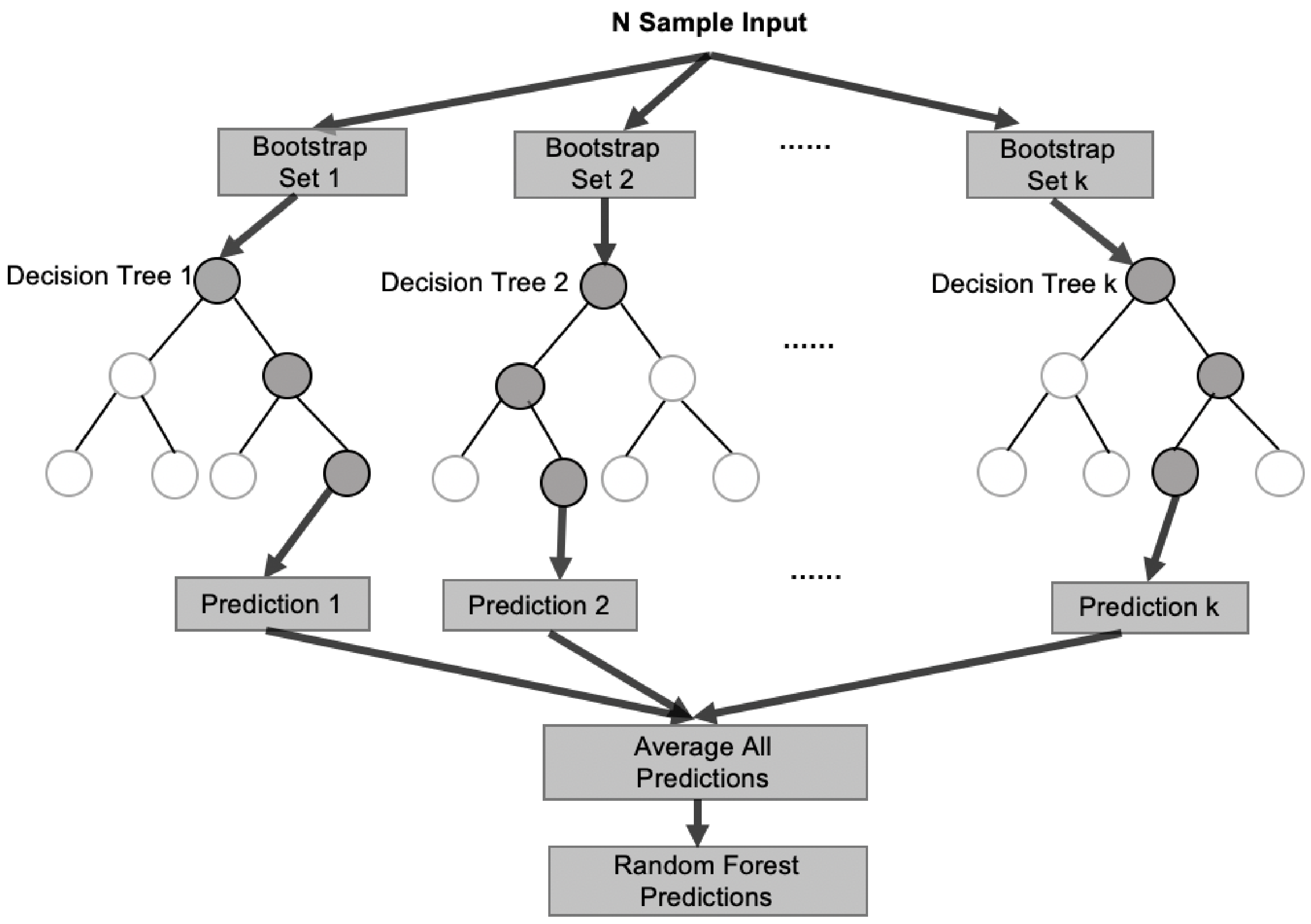
In this study, we utilize the random forest ensemble machine learning method to implement an inverse-modeling approach that uses the actual field production and injection data (measured at the surface) as the inputs to predict the time-lapse saturation profiles. Accurate estimation of fluid saturation is an important step in the dynamic reservoir characterization process, as it is one of the reservoir properties that changes over time and directly impacts well performance. Saturation measurements at a well location are useful for estimating remaining reserves, predicting production rates, planning workover activity, assessing drainage efficiency, performing economic analysis, and diagnosing production problems [1]. Traditionally, oil saturation at a wellbore location is estimated using wireline logging techniques such as thermal decay logging, carbon-oxygen logging, resistivity, etc. However, wireline logging suffers from several limitations such as production/injection interruption, tool operational limits, technical challenges in highly deviated wells, and the need to pull the tubing pump in some cases [9]. Well intervention can also be prohibitively expensive and operationally risky, especially in offshore environments and deviated well trajectories, which limits the frequency of data acquisition.

Machine learning techniques have been increasingly used in recent years for data-driven reservoir characterization, and specifically for saturation prediction, as summarized in

Table 1. Comparison of input/output features for machine learning-based saturation prediction studies.

Reference	Input	Output
This Study	Field Production and Injection data	Oil saturation
Miah et al. [15]	Well logs (Gamma Ray, Resistivity, Density, Neutron, Sonic Porosity)	Water saturation
Gholanlo et al. [16]	Well log (Sonic, Density, Neutron, Resistivity, Photoelectric Index)	Water saturation
Khan et al. [18]	Well log (Caliper, Gamma Ray, Density, Neutron Porosity, Resistivity)	Dean-stark data
Tariq et al. [19]	Well logs (Gamma Ray, Neutron Porosity, Bulk Density, Mobility)	Water saturation
Sambo et al. [23].	Seismic data (SQp and SQs attributes)	Fluid saturation
Ojukwu et al. [9]	Well logs (Density, Neutron, Sonic, Shale Volume), Seismic attributes, Production data, Core data (porosity, permeability)	Reservoir Quality (includes saturation)
Cao & Roy [24]	4D Seismic (Time-shift, Time strain, Amplitude), 3D Seismic (Acoustic Impedance, Porosity, Reservoir thickness)	Fluid Saturation
AI-Sudani [25]	Well logs (Resistivity, Porosity)	Water saturation
Tiwari et al. [26]	4D Seismic (Time-shift, Time strain, Amplitude), 3D Seismic (Acoustic Impedance, Amplitude, Density, Shear Impedance, Porosity, V-Shale, Facies), Production data	Fluid Saturation

. Several studies have utilized Neural Networks (NN) for predicting water or oil saturation using well logs and core data as inputs and demonstrated superior performance compared to conventional methods [10,11,12,13,14,15,16,17,18]. Algorithms such as functional networks [19], support vector machine [20], long short-term memory [21], and decision trees [22] have also been successfully used to predict fluid saturation in a variety of formation types using petrophysical well logs as input. The use of seismic data for estimating fluid saturations in machine learning models has also been reported [23,24]. Recently, researchers developed an analytical model to estimate water saturation by using capacitance-resistance model (CRM) and traditional resistivity logs [25]. Only a handful of studies [9,26] have incorporated production and injection data in the machine learning workflow for saturation prediction. However, these studies also require other input parameters derived from core, petrophysical logs, or seismic data. This limits the implementation of these models in field cases where such input data is not readily or reliably available, often due to the acquisition costs. A key distinction of this study is the use of only the field injection and production data, which are often readily available, as the key input feature for predicting time-lapse oil saturation profiles without requiring detailed geophysical inputs, as highlighted in Table 1.

Fluid production is an important reflection of the dynamic reservoir properties [27]. Moreover, production data is typically the most frequently and reliably measured quantity throughout the life of a field. Although oil saturation is influenced by a number of parameters such as the capillary pressure, drainage, injection, wettability, etc., the direct relationship between the changing reservoir fluid saturations and surface production can be illustrated from mass conservation as the production of fluids at the surface results in a change in reservoir saturations. However, it is a complex non-linear time-dependent relationship as the fluid saturation is affected by the field-wide drainage and injection over time. Supervised machine learning algorithms have been demonstrated to effectively “learn” the complex relationship between a given set of target prediction output and input features. In this study, a random forest ensemble machine learning algorithm is implemented using the actual field-wide production and injection data as the inputs, to predict the time-lapse wellbore oil saturation profiles. Static geological parameters such as absolute permeability, porosity, lithology, etc. are not included as input features because they do not typically change significantly over time at a given well location (except in some cases such as during fracking, high rate injection, and others) and they are also not measured frequently over the life of an operation. Other dynamic data such as downhole or surface pressures and temperatures are also not included as inputs to demonstrate the broad applicability of the algorithm when such data is not easily available, or not collected frequently.

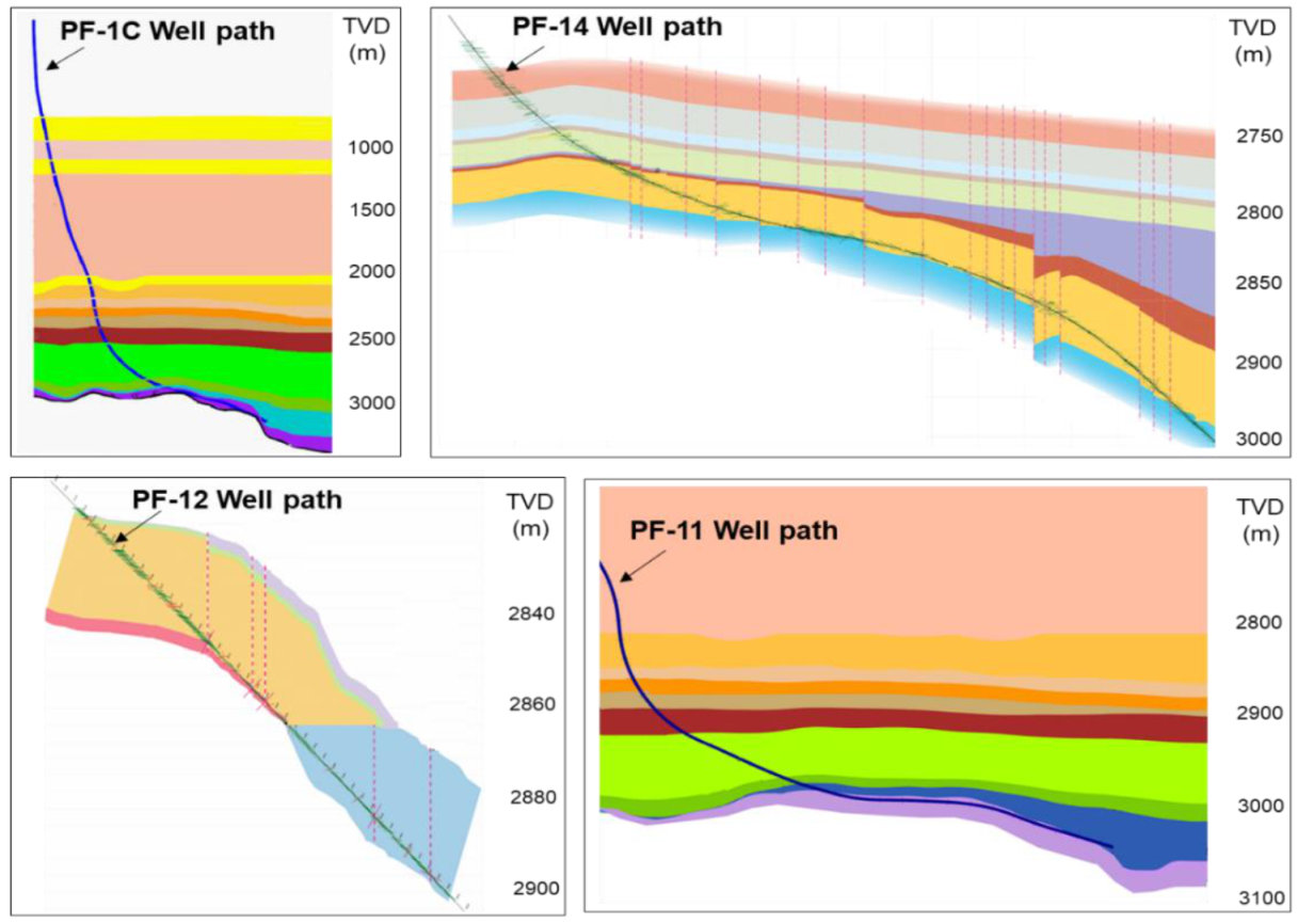
Since the time-lapsed oil saturation data is not collected in the subject offshore field, it is synthetically generated for training and testing the random forest algorithm through full-field numerical reservoir simulation. The simulation model is history-matched by adjusting reservoir parameters to ensure a reasonable agreement between the nine years of observed historical field behavior and simulation output, to establish a satisfactory representation of the field. Although the algorithm is demonstrated using synthetic saturation data, the workflow can also be implemented with actual field saturation profiles, if available. Three and a half years of historical field production, injection, and synthetic oil saturation trends (from the history-matched simulation model) are used for training, and about one year of data is used for the blind testing. The workflow is successfully demonstrated for predicting time-lapse saturation profiles at four deviated well locations, each representing a unique well trajectory, complex reservoir structure, and geological heterogeneity. In addition to demonstrating the workflow using the actual field production and injection data with simulated saturation data, it is also tested with the production, injection, and saturation data all from the simulation model. Very similar results are obtained (as illustrated in the Supplementary Material Figures S1 and S2) which is expected as the simulation model is history matched with the field data.

The next section describes the subject field and the available data, this is followed by the description of the machine learning algorithm and feature selection in Section 3, and the model prediction results and discussion in Section 4, and finally the conclusions in Section 5.

2. Field Overview and Data Description

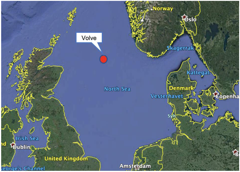
This study utilizes data from the Volve oil field, located in the central part of the North Sea, at the southern end of the Norwegian sector as shown in Figure 1. This offshore oil field was discovered in 1993, and the plan for development was approved in 2005 [28]. Field production started in early 2008, achieving 56,000 bbl/day of peak oil rate. New wells were drilled up until 2012–2013, which contributed to the increased recovery rate and extended life of the field. The main drainage strategy was pressure maintenance by water injection, with production wells placed high on the structure and water injectors at the flanks. The Volve field is described as a fault block structure with an initial estimation of 173 million bbl of oil in place [29]. The reservoir is a small dome-shaped structure and is believed to be formed due to the collapse of adjacent salt ridges during the Middle Jurassic age [29,30]. Oil was produced from the sandstone of Middle Jurassic age in the Hugin formation at an average depth of 2700 to 3100 m true vertical depth (TVD) below sea level. There is no known aquifer support, so the drainage was primarily dependent on reservoir depressurization and hydrocarbon displacement by water injection. The field was decommissioned in September 2016 after roughly nine years in operation that delivered a cumulative oil production of 63 million barrels, achieving a recovery rate of 54% [31].

Equinor (previously known as Statoil), the operator of Volve field, together with the Volve license partners released all subsurface and production datasets from the field in 2018 to support research, learning, and innovation for the energy future. The released dataset [29] includes production and injection data through the life of the operation (from 2008 to 2016), well trajectories, completion string design, seismic data, well logs (petrophysical and drilling), geological and stratigraphic data, static and dynamic models, surface and grid data.

For this study, the daily production and injection field data measured at the surface (from all six active producers and two active injectors) is used as input. Since saturation data is not measured directly in the Volve field, synthetic saturation profiles are generated using numerical reservoir simulation. A commercial simulator (CMG®) is used to create a black-oil heterogeneous reservoir model, as summarized in

Table 2. Reservoir simulation model parameters and well operating durations.

Number of Grid Blocks I, J, K	108, 100, 63
Grid Dimensions: dx, dy, dz (m)	50, 50, 1–3
Total Blocks (Active Cells)	680,400 (77,105)
Producers (Operating Duration)	PF-12 (2/2008–9/2016), PF-1C (4/2014–4/2016), PF-5 (4/2016–8/2016), PF-11(7/2013–9/2016), PF-14 (7/2008–7/2016), PF-15D (1/2014–/2016)
Injectors (Operating Duration)	IF-5 (8/2008–4/2016), IF-4 (4/2008–9/2016)

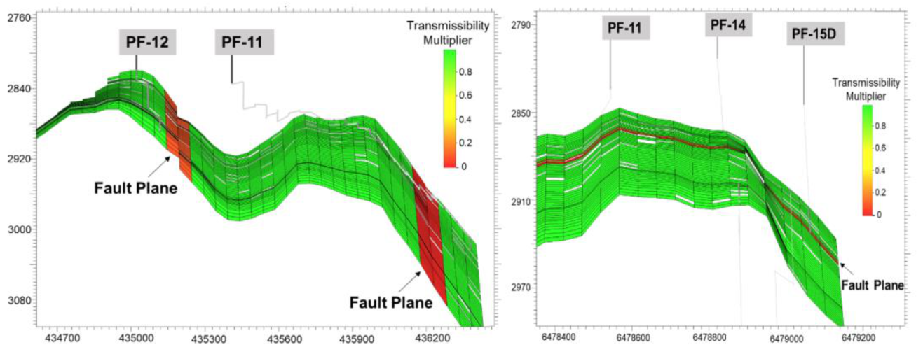
. The geological properties, well surveys, operating parameters, and grid dimensions are imported from the Eclipse^® simulation model that is part of Equinor’s publicly released Volve dataset [29]. The areal field map with the well locations is shown in Figure 2. The prefix “P” or “I” are added to the well names to indicate a producer or injector, respectively, as one of the injectors (well F-5) is converted into a producer later. The western part of the reservoir structure is heavily faulted, as shown in Figure 3, and communication across the faults is uncertain. The faults are represented using low transmissibility multipliers in the simulation model, consistent with the Volve simulation model developed by Equinor [32]. The oil, water, and gas production rates from the simulation model showed a reasonable match with the nine years of historical Volve field data, as illustrated in Figure 4 (where the monthly oil and water rates are expressed in thousands of stock tank barrels or MSTB, and the gas rate is expressed in millions of standard cubic feet or MMSCF). The objective of history matching is to ensure a reasonable representation of the Volve oil field. The saturation profiles from the history-matched simulation model, along with the actual field production (oil, water, gas) and injection (water) rates, are used for the training, validation, and testing of the ensemble machine learning model, as described in the next section. Although the algorithm is demonstrated using synthetic saturation data, the workflow can also be implemented with actual field saturation profiles, if available.

3. Materials and Methods

3.1. Random Forest Algorithm

This study implements a random forest algorithm which is a powerful machine learning method that uses the supervised ensemble approach for classification or regression [33]. It has been widely used in a variety of petroleum engineering applications, including for facies classification [34,35], well planning [36], and drilling optimization [37]. Information entropy and Gini Index are two criteria for random forest classification. Entropy is a measure of disorder or uncertainty and defined mathematically as:

$$E\left(S\right)= -{\displaystyle \sum }_{i=1}^c{p}_i{\log }_2{p}_i$$

(1)

In this equation p_i is the frequentist probability of an element/class i in data. Gini Index (I_G), also known as Gini impurity, calculates the amount of probability of a specific feature that is classified incorrectly when selected randomly. It is defined as:

$$I_G=1-{\displaystyle \sum }_{i=1}^c{\left(p_i\right)}^2$$

(2)

In this equation p_i denotes the probability of an element being classified for a distinct class. While information entropy and Gini Index are common criterion functions for classification trees, mean squared error (MSE) and mean absolute error (MAE) are commonly used for regression trees. MSE measures the average of the squares of the difference between the actual and predicted values and defined mathematically as:

$$MSE={{\displaystyle \sum }}_{i=1}^n{\left(y_i - f\left(x_i\right)\right)}^2/n$$

(3)

whereas MAE represents the difference between the absolute difference between the actual and predicted values averaged over the dataset and given by:

$$MAE={{\displaystyle \sum }}_{i=1}^n|y_i - f\left(x_i\right)|/n$$

(4)

Random forest utilizes a bagging technique by sampling with replacement from the original dataset randomly to construct bootstrapped datasets. The algorithm operates by using these bootstrapped datasets to create decision trees and gives prediction from the mean values of each tree, as illustrated in the schematic in Figure 5. At each node of a regression tree, a random subset of all input variables is selected as candidates for binary partitioning [38]. The regression tree splitting criterion is based on the criterion function that measures the quality of a split, based on which the best candidate is used to split the current node. The predicted value of an observation is calculated by averaging over all the trees.

In this study, the Scikit-learn package in Python is used as the framework to build the random forest model [39]. Scikit-learn module integrates a wide range of machine learning algorithms for medium-scale supervised and unsupervised problems. Several hyperparameters in the model are tuned to improve the predictive power, generalizability, and robustness of the model. The ‘model_selection’ package in Scikit-learn combined with the training dataset are used to find the best hyperparameters for the random f model. The optimum random forest hyperparameters are shown in

Table 3. Optimum hyperparameters for the random forest model.

N_Estimators	Max_Features	Max_Depth	Min_Samples_Split	Max_Leaf_Nodes	Criterion
20	auto	none	2	None	MSE

. For instance, n_estimators represent the number of trees in the forest and it is set to 20 to avoid underfitting and optimize the computational time. Typically, the higher number of trees gives the better prediction, however, adding a lot of trees can slow down the training process. The max_features determines the number of input variables to consider when looking for the best split and a value of “auto” is set which means all the input features are used for the model. MSE is used the criterion function to measure the quality of a split which implies variance reduction as the feature selection criterion. The max_depth is the hyperparameter to limit the depth of the subtree when it builds the random forest model. The min_samples_split limits the conditions for the subtree to continue to be divided. If the number of samples of a node is less than the value, it will not continue to try to select the optimal feature for the division. In view of the dataset size, the max_depth and min_samples_split are set as default. The max_leaf_nodes is used to prevent overfitting, we selected "None" which represent the maximum number of leaf nodes is not limited. The model performance is evaluated using the R-square (R2), root mean square error (RMSE) and mean absolute percentage error (MAPE). R-square is a statistical measure of how close the data are to the fitted regression line. It is defined by the percentage of explained variation on total variation. The total variation about a regression line is the sum of the squares of the differences between the y-value of each ordered pair and the mean of y, that is $\sum \left(y-\overline{y}\right)$². The explained variation is the sum of the squared of the differences between each predicted y-value and the mean of y, that is $\sum \left(\widehat{y}-\overline{y}\right)$². It is also known as the coefficient of determination, or the coefficient of multiple determination for multiple regression. RMSE is a measure of how spread out these residuals are. It is the standard deviation of the residuals (prediction errors). It is defined by the error rate by the square root of MSE. Residuals are a measure of how far from the regression line data points are. MAPE is a statistical measure of how accurate a forecast model is. It measures this accuracy as a percentage and can be calculated as the average absolute percent error for each time period minus actual values divided by actual values. MAPE is the another common measure used to forecast error and works best if there are no extremes to the data (and no zeros). R-square by itself does not indicate whether the coefficient estimates and predictions are biased, which is why we also need to assess the RMSE which is the standard deviation of the prediction errors. In other words, it tells us how concentrated the data is around the line of best fit.

3.2. Data Preparation and Feature Selection

The input features in the random forest model are the actual field-wide injection (water) and production (oil, water, gas) history, while the output is time-lapsed oil saturation versus depth profile at a well location, which is generated using history-matched reservoir simulation. Nearly five years of data from 2011 to 2016 is used in this study. The entire dataset is divided into training, validation, and test sets. The first 3.6 years of production, injection, and saturation history (from November 2011 to June 2015) is randomly divided for training and validation with an 80% and 20% split, respectively, while the last 1.25 years of data (from July 2015 to October 2016) is used for the blind testing. The workflow is demonstrated for predicting saturation profiles at four producer well locations: PF-1C, PF-14, PF-12, and PF-11. Each well has a unique deviated well trajectory as shown in Figure 6. The geological structure and reservoir heterogeneity (demonstrated through the vertical permeability in millidarcy or mD) at the four test-well locations are shown in Figure 7. These figures highlight the complex reservoir architecture, unique well paths, and geological heterogeneity present at each well location that is used to demonstrate the workflow.

The dynamic oil saturation profile at a well location is affected by the injection and production in the surrounding wells. Therefore the model inputs included actual field production (oil, water, gas) rates for the target well as well as the injection (water) and production (oil, water, gas) from the surrounding wells, in addition to the time, and depth measured across the producing interval. The output is oil saturation profile across the producing interval along the wellbore, which is compared with the saturation data generated from the simulation model. The gas saturation in the reservoir is negligible and therefore it is not modeled. The production and injection data are measured daily in the field, while the oil saturation profiles are recorded from the simulation model every 10 to 15 days, at unequal time steps. The data frequency reflects actual field conditions where the production and injection are measured or allocated daily, while the oil saturation profile is typically measured using wireline logs or estimated analytically every few days, months or years, depending on the operational requirements. Instead of using the production and injection rates only on the day of the saturation measurement, the daily rate data is averaged over the previous ten days to synchronize with the temporal frequency of the oil saturation data. The averaging is done to account for any temporary fluctuations in the daily rates due to the surface operating conditions and to accurately reflect the reservoir-driven production and saturation changes. Because of the highly dipping reservoir structure (Figure 7), some grid blocks in the simulation model are pinched out (due to thickness less than 10⁻⁴ m) and therefore removed during the data preparation. The final data are divided into training, validation, and test sets. The number of data points for each dataset is summarized in

Table 4. Dataset partition for the random forest model.

	PF-1C	PF-14	PF-12	PF-11
Training dataset	23680	18648	5835	14644
Validation dataset	5921	4661	1458	3660
Test dataset	9264	7824	2448	6144

which are based on the data separation methodology described in the previous paragraph. The range of the production and injection data for all wells is summarized in

Table 5. The range of all input features used in the machine learning model (oil and water rates in MSTB/day, gas rates in MSCF/day).

Well Name	Inputs Feature	Range of Inputs
PF-1C	Oil/Water/Gas Rate	(0–9.7)/(0–10.3)/(0–7828)
PF-11	Oil/Water/Gas Rate	(0–12.9)/(0–22.4)/(0–10598)
PF-12	Oil/Water/Gas Rate	(0–8.6)/(0–40.2)/(0–7356)
PF-14	Oil/Water/Gas Rate	(0–12.7)/(0–30.5)/(0–10845)
PF-15D	Oil/Water/Gas Rate	(0–3.2)/(0–2.2)/(0–2740)
IF-4	Water Injection Rate	(0–55.8)
IF-5	Water Injection Rate	(0–51.5)

. The saturation data corresponds to the saturation values in the simulation grid blocks intersected by the wellbore in the reservoir zone, as illustrated in Figure 8a. The initial oil saturation profile across the four wellbores is illustrated in Figure 8b. Corresponding to each time-step, there will be a single production and injection value but multiple saturation values along with the measured depth of the well, which results in a large dataset in Table 4 (this is also demonstrated with an example in the Supplementary Figure S3).

3.3. Feature Selection

To improve the computational efficiency and performance of the model, a feature selection analysis is performed to select the wells that are most influential in predicting the saturation at the four test-well locations. This is done by evaluating the input data correlation and feature importance ranking. The Pearson correlation coefficient (r) is used to measure the strength of the linear association between two variables given by:

$$r= \sum \left(x_i-\overline{x}\right)\left(y_i-\overline{y}\right)/\sqrt{\sum {\left(x_i-\overline{x}\right)}^2\sum {\left(y_i-\overline{y}\right)}^2}$$

(5)

where x_i and y_i are the actual values, and $\overline{x}, \overline{y}$ are the mean of the values. Two variables have a high correlation if a change in one variable affects a similar change in another at the same time [40]. A value of r = 1 means a perfect positive correlation, while r = −1 indicates a perfect negative correlation. Pearson’s correlation coefficient is calculated for the oil, water, and gas rate attributes between each well pair to analyze the effect of production or injection in one well on the rates in the other well. The absolute values of the correlation coefficients for oil, water, and gas rates are aggregated at the well level to reflect the statistical relationship between the well pairs.

The feature importance is calculated by evaluating the relative contribution of each input feature in predicting the output, which also takes into account any non-linear relationship [41]. Tree-based models provide a measure of feature importance based on the mean decrease in impurity (MDI). Impurity is quantified by the splitting criterion of the decision trees (Gini, entropy, or MSE). Even though impurity-based feature importance for trees is strongly biased, it favors high cardinality features (typically numerical features) over low cardinality features such as binary features or categorical variables. The contribution is based on impurity, which in the case of regression problems is variance. The individual scores calculated for the oil, water, and gas rate attributes are summed up for each well to reflect the total feature importance score for the well in predicting the output (oil saturation) at the test-well location.

The final set of input features for the random forest model are selected based on the agreement between the Pearson correlation coefficient, feature importance scores, and the domain-knowledge such as the structural location of the injectors and the producers, geological features such as reservoir dip and proximity to faults, as demonstrated in Figure 9. The input features of time and depth are included in all models and not included in feature importance evaluation since they are fundamentally needed for generating the temporal and spatial saturation profile.

4. Results and Discussion

4.1. Feature Selection Results

Figure 10 shows the correlation matrix for all well pairs which is calculated by aggregating the absolute values of the Pearson correlation coefficients for oil, water, and gas rate attributes at the well level. The feature importance scores estimated for each test well are presented in Figure 11. The final input variables for the random forest model are determined based on the results from the pair-wise Pearson’s correlation, feature importance results, as well as the underlying geological understanding, as summarized in

Table 6. Input variables for the predictive random forest model for each test-well.

Features	Test Wells
	PF-1C	PF-14	PF-12	PF-11
PF-1C (oil, water, gas rates)	✓	✓		✓
PF-5 (oil, water, gas rates)
PF-11 (oil, water, gas rates)	✓	✓	✓	✓
PF-12 (oil, water, gas rates)	✓	✓	✓	✓
PF-14 (oil, water, gas rates)	✓	✓	✓	✓
PF-15D (oil, water, gas rates)	✓	✓	✓	✓
IF-4 (water injection rate)		✓	✓	✓
IF-5 (water injection rate)		✓	✓	✓
Time	✓	✓	✓	✓
Depth	✓	✓	✓	✓

. When a feature (such a well) is not included, we just didn’t include the corresponding production and injection values in the input matrix. For instance, for well PF-1C, wells PF-5, IF-4, and IF-5 are not included as input features because they had a low correlation with PF-1C (Figure 10), low feature importance (Figure 11), and they are also located farthest from well PF-1C (Figure 2). Both the injectors (IF-4 and IF-5) are structurally neither on strike nor directly downdip of PF-1C as illustrated in the 3D view of the horizontal permeability in Figure 10 (left), which justifies minimal impact from a geological standpoint. For well PF-14, only well PF-5 is excluded as it met all three criteria of low correlation coefficient (Figure 10), low feature importance (Figure 11), and geological distance (Figure 12). For well PF-11, even though the two injectors (IF-4 and IF-5) ranked low on feature importance and correlation coefficient, they are included as input features as they are located directly downdip of PF-11, as shown in Figure 10 (right). Thus, from a geological standpoint, they are expected to influence the saturation profile at PF-11. The data from well PF-5 ranked very low in both the feature importance score and correlation coefficients, as this well produced for only four months (see Table 2).

4.2. Oil Saturation Prediction Results

In order to find the optimal machine learning method for saturation prediction six different standard regression algorithms are tested namely, linear regression [42], K-neighbors [43], multi-layer perceptron [44], gradient boosting [45], AdaBoost [46], and random forest. All the models are used from Scikit-learn package in Python directly. To simplify the model comparison process, the performance is tested on one of the four test-wells (PF-12). Consistent with the methodology described in Sec. 3.2, the first 3.6 years of production, injection, and saturation history (from November 2011 to June 2015) is randomly divided for training and validation with an 80% and20% split, respectively, while the last 1.25 years of data (from July 2015 to October 2016) is used for the blind testing. The training dataset is used for grid search. The model_selection package from Scikit-learn [39] which includes GridSearchCV and grid.fit methods are used to find the best hyperparameters for each model which are shown in (Supplementary File Tables S1–S4). After tuning the hyperparameters, 1.5 years blind testing data are used for predicting oil saturation for PF-12. The performances of the different models are summarized in

Table 7. The performance of different machine learning models on PF-12.

	Linear	Random Forest	K-Neighbors	Ada Boost	Gradient Boosting
MAPE	0.1917	0.0486	0.1944	0.1629	0.0745
RMSE	0.1507	0.0324	0.1298	0.0856	0.0675
R2	−0.1036	0.9142	0.1801	0.6439	0.8563

. Based on ANOVA analysis (included in the Supplementary Figure S4) the difference between the model results are statistically significant. Random forest demonstrated the best prediction performance (highest R-square, lowest RMSE, and lowest MAPE), followed by gradient boosting and AdaBoost. The MAPE and RMSE scores are expressed in the same unit as the saturation, which is a fraction. Based on the assessment, Random forest algorithm was selected for saturation modeling at all four test well locations.

The selected input features (Table 6) are used to train, validate, and test the Random forest model for each of the four test-wells (PF-1C, PF-14, PF-12, and PF-11). To further illustrate the role of feature selection, the model also tests four wells by including all features before the feature selection process as input. The comparison of the resulting performance of the model prediction using the MAPE, RMSE and R-square is summarized in

Table 8. Comparison of performance with and without removed input features for each test-well based on the average of 35 independent model runs.

Metric (Selected/All Features)	PF-1C	PF-14	PF-12	PF-11
MAPE	0.0542/0.0523	0.0397/0.0398	0.0532/0.0486	0.0642/0.0654
RMSE	0.0513/0.0534	0.0291/0.0298	0.0387/0.0324	0.0554/0.0554
R2	0.9312/0.9331	0.9567/0.9543	0.9212/0.9142	0.9365/0.9756
Computation Time (seconds)	4.1700/4.6823	3.8482/4.1938	1.5023/1.6130	2.9332/3.3412

. The results are based on running 35 independent runs, and the standard deviation of the results are shown in

Table 9. Standard deviation in performance metrics for the 35 independent random forest model runs for each test-well.

	PF-1C	PF-14	PF-12	PF-11
MAPE (Selected/All Features)	0.00039/0.00038	0.00042/0.00039	0.00043/0.00041	0.00042/0.00039
RMSE (Selected/All Features)	0.00050/0.00054	0.00051/0.00053	0.00051/0.00052	0.00053/0.00053
R2 (Selected/All Features)	0.00153/0.00156	0.00153/0.00156	0.00151/0.00157	0.00154/0.00156

. It could be seen from each column that by including the removed wells, the results remain unchanged. The feature selection provides efficiency by reducing computation time as well as data preparation time by elimination of redundant features. The model computation time before and after the feature selection are different as summarized in Table 8. The results also show that the model predicts time-lapse oil saturation profiles with over 90% R-square, less than 0.07 MAPE and less than 0.06 RMSE in all cases. The predicted and actual values of oil saturation for the entire testing dataset for each well are presented in Figure 13. The majority of the predicted values overlap the actual data points, which shows that the regression model reasonably forecasts the change of oil saturation. However, the model shows low R-square for some data points. One of the main factors influencing the mismatch between the actual and predicted saturation at certain depths is the intersection of well path with the fault boundaries, which creates flow barrier and discontinuities making it difficult for the machine learning model to predict the saturation trend accurately. This is demonstrated in Figure 14 which illustrates the well paths intersecting the fault planes that are modeled as low transmissibility zones in the simulation model.

To demonstrate the performance of the random forest model in predicting the time-lapse saturation profile trends, the actual and predicted saturation profiles for representative time steps from the testing dataset are compared in Figure 15 for all four test-wells. The three time-steps correspond to the starting of the test-set (7/3/2015), middle (2/8/2016), and the end of test-set (9/5/2016). To illustrate the change in oil saturation over a longer duration two additional saturation profiles (11/1/2011 and 10/6/2012) are included in the left two plots of Figure 15. In each figure, the blue curve represents the actual saturation values (obtained from the reservoir simulation), while the red curves represent the predicted saturation values from the random forest model. The results show a reasonable saturation prediction in all cases with acceptable errors. Not all saturation changes are fully captured at some intervals likely due to the complex reservoir structure, faulting, and the limited number of input features used in the random forest model. However, the results clearly demonstrate the effectiveness of our simple modeling approach utilizing the most readily available field injection and production data as the primary inputs in predicting time-lapse saturation profile within acceptable error margins in a structurally complex and heterogeneous reservoir.

5. Conclusions

In this study, we develop an ensemble machine learning method to implement an inverse-modeling approach that uses the field-wide production and injection data as the main inputs to predict the time-lapse saturation profiles. Other dynamic reservoir parameters such as pressures, temperatures, and static geological attributes such as permeability, porosity, etc. are not included as inputs to demonstrate the broad applicability of the algorithm when such data is not easily or reliably available. The workflow is demonstrated using actual field injection and production data measured at the surface from a structurally complex, heterogeneous, and heavily faulted offshore oil field. The oil saturation data for training and testing the machine learning model is synthetically generated through full-field history-matched numerical reservoir simulation, as time-lapsed saturation data is not measured directly in the subject field.

The random forest model predicted dynamic saturation profiles at four deviated well locations, each representing a unique well trajectory, complex reservoir structure, and geological heterogeneity, with over 90% R-square, less than 0.07 MAPE and less than 0.06 RMSE in all cases. The results demonstrate the effectiveness of our simple and intuitive modeling approach that captures the dynamic relationship between the field production, injection, and oil saturation trends.

The proposed workflow is demonstrated for a waterflood operation but it can also be adopted for primary production, which will be a special case for no water injection. For other enhanced oil recovery (EOR) processes (such as polymer, steam, or gas injection), the key criteria that will determine whether or not our model can be applied are the recovery mechanisms. For instance, if a process significantly alters the reservoir properties, like permeability (in case of fracking) or temperatures (in case of a steam flood) then the model will need to incorporate those changes, as the current model does not include permeability or temperature as an input feature. This study uses simulated oil saturation data. In the future, we plan to extend this by using saturation data from well logs and also implement the workflow in other oil and gas fields.

References

1. Baker, R.O.; Yarranton, H.W.; Jensen, J.L. 1—Introduction. In Practical Reservoir Engineering and Characterization; Baker, R.O., Yarranton, H.W., Jensen, J.L., Eds.; Gulf Professional Publishing: Boston, MA, USA, 2015; pp. 1–32. [Google Scholar] [CrossRef]
2. Luo, G.; Tian, Y.; Bychina, M.; Ehlig-Economides, C. Production-Strategy Insights Using Machine Learning: Application for Bakken Shale. SPE Reserv. Eval. Eng. 2019, 22, 800–816. [Google Scholar] [CrossRef]
3. Fulford, D.S.; Bowie, B.; Berry, M.E.; Bowen, B.; Turk, D.W. Machine Learning as a Reliable Technology for Evaluating Time-Rate Performance of Unconventional Wells. In Proceedings of the SPE Annual Technical Conference and Exhibition, Houston, TX, USA, 28 September 2015; p. 29. [Google Scholar]
4. Berneti, S.; Shahbazian, M. An Imperialist Competitive Algorithm Artificial Neural Network Method to Predict Oil Flow Rate of the Wells. Int. J. Comput. Appl. 2011, 26, 47–50. [Google Scholar] [CrossRef]
5. Cao, Q.; Banerjee, R.; Gupta, S.; Li, J.; Zhou, W.; Jeyachandra, B. Data Driven Production Forecasting Using Machine Learning. In Proceedings of the SPE Argentina Exploration and Production of Unconventional Resources Symposium, Buenos Aires, Argentina, 1 June 2016; p. 10. [Google Scholar]
6. Martin, E.; Wills, P.; Hohl, D.; Lopez, J.L. Using Machine Learning to Predict Production at a Peace River Thermal EOR Site. In Proceedings of the SPE Reservoir Simulation Conference, Montgomery, TX, USA, 20 February 2017; p. 8. [Google Scholar]
7. Mukherjee, T.; Burgett, T.; Ghanchi, T.; Donegan, C.; Ward, T. Predicting gas production using machine learning methods: A case study. In Proceedings of the SEG International Exposition and Annual Meeting, San Antonio, TX, USA, 25 September 2019; p. 5. [Google Scholar]
8. Balashov, D.; Egorov, D.; Belozerov, B.; Slivkin, S. Prediction of Wells Productive Characteristics with the Use of Unsupervised Machine Learning Algorithms. In Proceedings of the SPE Russian Petroleum Technology Conference, Moscow, Russia, 22 October 2019; p. 12. [Google Scholar]
9. Ojukwu, C.; Smith, K.; Kadkhodayan, N.; Leung, M.; Baldwin, K. Reservoir Characterization, Machine Learning and Big Data—An Offshore California Case Study. In Proceedings of the SPE Nigeria Annual International Conference and Exhibition, Virtual, 11–13 August 2020; p. 13. [Google Scholar]
10. Roueché, J.N.; Karacan, C.Ö. Zone Identification and Oil Saturation Prediction in a Waterflooded Field: Residual Oil Zone, East Seminole Field, Texas, USA, Permian Basin. In Proceedings of the SPE Improved Oil Recovery Conference, Tulsa, OK, USA, 14 April 2018; p. 14. [Google Scholar]
11. Shokir, E.M.E.-M. Prediction of the Hydrocarbon Saturation in Low Resistivity Formation via Artificial Neural Network. In Proceedings of the SPE Asia Pacific Conference on Integrated Modelling for Asset Management, Kuala Lumpur, Malaysia, 1 January 2004; p. 6. [Google Scholar]
12. Al-Bulushi, N.; Araujo, M.; Kraaijveld, M.; Jing, X.D. Predicting Water Saturation Using Artificial Neural Networks (ANNs). In Proceedings of the SPWLA Middle East Regional Symposium, Abu Dhabi, UAE, 1 January 2007; p. 16. [Google Scholar]
13. Helle, H.B.; Bhatt, A. Fluid saturation from well logs using committee neural networks. Pet. Geosci. 2002, 8, 109–118. [Google Scholar] [CrossRef]
14. Goda, H.M.; Maier, H.; Behrenbruch, P. The Development of an Optimal Artificial Neural Network Model for Estimating Initial Water Saturation—Australian Reservoir. In Proceedings of the SPE Asia Pacific Oil and Gas Conference and Exhibition, Jakarta, Indonesia, 1 January 2005; p. 15. [Google Scholar]
15. Miah, M.I.; Ahmed, S.; Zendehboudi, S. Connectionist and mutual information tools to determine water saturation and rank input log variables. J. Pet. Sci. Eng. 2020, 190, 106741. [Google Scholar] [CrossRef]
16. Gholanlo, H.H.; Amirpour, M.; Ahmadi, S. Estimation of water saturation by using radial based function artificial neural network in carbonate reservoir: A case study in Sarvak formation. Petroleum 2016, 2, 166–170. [Google Scholar] [CrossRef] [Green Version]
17. Miah, M.I.; Zendehboudi, S.; Ahmed, S. Log data-driven model and feature ranking for water saturation prediction using machine learning approach. J. Pet. Sci. Eng. 2020, 194, 107291. [Google Scholar] [CrossRef]
18. Khan, M.R.; Tariq, Z.; Abdulraheem, A. Machine Learning Derived Correlation to Determine Water Saturation in Complex Lithologies. In Proceedings of the SPE Kingdom of Saudi Arabia Annual Technical Symposium and Exhibition, Dammam, Saudi Arabia, 23–26 April 2018. [Google Scholar]
19. Tariq, Z.; Mahmoud, M.; Abdulraheem, A. An intelligent data-driven model for Dean–Stark water saturation prediction in carbonate rocks. Neural Comput. Appl. 2020, 32, 11919–11935. [Google Scholar] [CrossRef]
20. Mollajan, A.; Memarian, H.; Jalali, M.R. Prediction of Reservoir Water Saturation Using Support Vector Regression in an Iranian Carbonate Reservoir. In Proceedings of the 47th U.S. Rock Mechanics/Geomechanics Symposium, San Francisco, CA, USA, 1 January 2013; p. 6. [Google Scholar]
21. Zhang, Q.; Wei, C.; Wang, Y.; Du, S.; Zhou, Y.; Song, H. Potential for Prediction of Water Saturation Distribution in Reservoirs Utilizing Machine Learning Methods. Energies 2019, 12, 3597. [Google Scholar] [CrossRef] [Green Version]
22. Baziar, S.; Shahripour, H.B.; Tadayoni, M.; Nabi-Bidhendi, M. Prediction of water saturation in a tight gas sandstone reservoir by using four intelligent methods: A comparative study. Neural Comput. Appl. 2018, 30, 1171–1185. [Google Scholar] [CrossRef]
23. Sambo, C.H.; Hermana, M.; Babasari, A.; Janjuhah, H.T.; Ghosh, D.P. Application of Artificial Intelligence Methods for Predicting Water Saturation from New Seismic Attributes. In Proceedings of the Offshore Technology Conference Asia, Kuala Lumpur, Malaysia, 20 March 2018; p. 8. [Google Scholar]
24. Cao, J.; Roy, B. Time-lapse reservoir property change estimation from seismic using machine learning. Lead. Edge 2017, 36, 234–238. [Google Scholar] [CrossRef]
25. Al-Sudani, J.A.; Mustafa, H.K.; Al-Sudani, D.F.; Falih, H. Analytical water saturation model using capacitance-resistance simulation: Clean and shaly formations. J. Nat. Gas Sci. Eng. 2020, 82, 103325. [Google Scholar] [CrossRef]
26. Tiwari, U.; Roy, B.; Cardozo, L.E. SAGD dynamic reservoir property characterization using machine learning. In Proceedings of the 2018 SEG International Exposition and Annual Meeting, Anaheim, CA, USA, 30 November 2018; p. 5. [Google Scholar]
27. Yang, H.; Gao, Y.; Yang, A.-P. Application of Well Production Data to Reservoir Characterization. In Proceedings of the SPE Annual Technical Conference and Exhibition, Dallas, TX, USA, 1 January 1995; p. 14. [Google Scholar]
28. Sen, S.; Ganguli, S.S. Estimation of Pore Pressure and Fracture Gradient in Volve Field, Norwegian North Sea. In Proceedings of the SPE Oil and Gas India Conference and Exhibition, Mumbai, India, 8 April 2019; p. 8. [Google Scholar]
29. Equinor. Volve Field Dataset. Available online: https://data.equinor.com/dataset/Volve (accessed on 11 September 2020).
30. Szydlik, T.J.; Way, S.; Smith, P.; Aamodt, L.; Friedrich, C. 3D PP/PS Prestack Depth Migration on the Volve Field. In Proceedings of the 68th EAGE Conference and Exhibition incorporating SPE EUROPEC 2006, Vienna, Austria, 12–15 June 2006. [Google Scholar] [CrossRef]
31. Equinor Volve Field. 2020. Available online: https://www.equinor.com/en/what-we-do/norwegian-continental-shelf-platforms/volve.html (accessed on 14 August 2020).
32. Equinor. 2016. Volve Reservoir Model and History Match Report. Available online: https://data.equinor.com/dataset/Volve (accessed on 14 August 2020).
33. Breiman, L. Random Forests. Mach. Learn. 2001, 45, 5–32. [Google Scholar] [CrossRef] [Green Version]
34. Kim, Y.; Hardisty, R.; Torres Parada, E.; Marfurt, K. Seismic-Facies Classification Using Random Forest Algorithm; Society of Exploration Geophysicists: Tulsa, Okla, USA, 2018; pp. 2161–2165. [Google Scholar] [CrossRef]
35. Deng, T.; Xu, C.; Jobe, D.; Xu, R. A Comparative Study of Three Supervised Machine-Learning Algorithms for Classifying Carbonate Vuggy Facies in the Kansas Arbuckle Formation. Petrophysics 2019, 60, 838–853. [Google Scholar]
36. Aulia, A.; Rahman, A.; Quijano Velasco, J.J. Strategic Well Test Planning Using Random Forest. In Proceedings of the SPE Intelligent Energy Conference & Exhibition, Utrecht, The Netherlands, 1 April 2014; p. 23. [Google Scholar]
37. Hegde, C.; Wallace, S.; Gray, K. Using Trees, Bagging, and Random Forests to Predict Rate of Penetration during Drilling. In Proceedings of the SPE Middle East Intelligent Oil and Gas Conference and Exhibition, Abu Dhabi, UAE, 15 September 2015; p. 12. [Google Scholar]
38. Wang, L.a.; Zhou, X.; Zhu, X.; Dong, Z.; Guo, W. Estimation of biomass in wheat using random forest regression algorithm and remote sensing data. Crop J. 2016, 4, 212–219. [Google Scholar] [CrossRef] [Green Version]
39. Pedregosa, F.; Varoquaux, G.; Gramfort, A.; Michel, V.; Thirion, B.; Grisel, O.; Blondel, M.; Prettenhofer, P.; Weiss, R.; Dubourg, V. Scikit-learn: Machine Learning in Python. J. Mach. Learn. Res. 2011, 12, 2825–2830. [Google Scholar]
40. Tsai, C.-F. Feature selection in bankruptcy prediction. Knowl. Based Syst. 2009, 22, 120–127. [Google Scholar] [CrossRef]
41. Nguyen, T.-T.; Huang, J.Z.; Nguyen, T.T. Unbiased Feature Selection in Learning Random Forests for High-Dimensional Data. Sci. World J. 2015, 471371. [Google Scholar] [CrossRef] [PubMed]
42. Kumari, K.; Yadav, S. Linear regression analysis study. J. Pract. Cardiovasc. Sci. 2018, 4, 33. [Google Scholar] [CrossRef]
43. Anava, O.; Levy, K.Y. k*-Nearest Neighbors: From Global to Local. In Proceedings of the NIPS, Barcelona, Spain, 5–10 December 2016. [Google Scholar]
44. Murtagh, F. Multilayer perceptrons for classification and regression. Neurocomputing 1991, 2, 183–197. [Google Scholar] [CrossRef]
45. Zemel, R.; Pitassi, T. A Gradient-Based Boosting Algorithm for Regression Problems. In Advances in Neural Information Processing Systems; MIT Press: Cambridge, MA, USA, 2001; pp. 696–702. [Google Scholar]
46. Shapire, R. A decision-Theoretic generalization of on-line learning and an application to boosting. J. Comp. Syst. Sci. 1995, 55, 119–139. [Google Scholar]
Figure 1. The geographic location of the Volve field.
Energies 14 01052 g001
Figure 2. Areal grid-top map of the Volve field showing the surface locations of the injectors and producers (X and Y axis represent the UTM coordinates in meters and colors represent the grid-top depth in meters).
Energies 14 01052 g002
Figure 3. Perspective view of the major faults in the Volve field which are highlighted here as solid red lines (Equinor, 2016).
Energies 14 01052 g003
Figure 4. History matching results from the CMG® simulation model used in this study and comparison with the field oil, water, and gas production rates.
Energies 14 01052 g004
Figure 5. The process of building a random forest ensemble.
Energies 14 01052 g005
Figure 6. Well trajectories for the four test-wells used in this study for demonstrating the random forest workflow (colors indicate different reservoir formations targeted by the wellbore) [29].
Energies 14 01052 g006
Figure 7. Cross-sections from simulation model highlight the reservoir structure and vertical permeability variation at the four test-well locations (Y-axis is TVD in meters and X-axis is UTM coordinates in meters).
Energies 14 01052 g007
Figure 8. (a) Saturation from grid block intersected by the well (b) Initial oil saturation profiles at the four test wells.
Energies 14 01052 g008
Figure 9. Feature selection based on agreement between data correlation, feature importance, and domain knowledge.
Energies 14 01052 g009
Figure 10. Correlation matrix for all well pairs.
Energies 14 01052 g010
Figure 11. The feature importance for each test-well.
Energies 14 01052 g011
Figure 12. 3D reservoir view showing the horizontal permeability (in mD) and structural location of injector wells IF-4 and IF-5 with respect to well PF-1C (left) and PF-11 (right).
Energies 14 01052 g012
Figure 13. Performance of random forest on test data.
Energies 14 01052 g013
Figure 14. Intersection of well paths with faults which are modeled as low transmissibility grids in the simulation model.
Energies 14 01052 g014
Figure 15. Predicted (red curves) versus the actual (blue curves) time-lapsed oil saturation profiles at the four test-well locations.
Energies 14 01052 g015