
Longitudinal Dynamics Simulation Tool for Hybrid APU and Full Electric Vehicle


Department of Mechanical and Industrial Engineering, University of Brescia, I-25123 Brescia, Italy
*
Author to whom correspondence should be addressed.
Energies 2021, 14(4), 1207; https://0-doi-org.brum.beds.ac.uk/10.3390/en14041207
Submission received: 28 January 2021
/
Revised: 11 February 2021
/
Accepted: 17 February 2021
/
Published: 23 February 2021
(This article belongs to the Special Issue Vehicle Dynamics and Control)
Abstract
:Due to problems related to environmental pollution and fossil fuels consumption that have not infinite availability, the automotive sector is increasingly moving towards electric powertrains. The most limiting aspect of this category of vehicles is certainly the battery pack, regarding the difficulty in obtaining high range with good performance and low weights. The aim of this work is to provide a simulation tool, which allows for the analysis of the performance of different types of electric and hybrid powertrains, concerning both mechanical and electrical aspects. Through this model it is possible to test different vehicle configurations before prototype realization or to investigate the impact that subsystems’ modifications may have on a vehicle under development. This will allow to speed-up the model-based design process typical for fully electric and hybrid vehicles. The model aims to be at the same time complete but simple enough to lower the simulation time and computational burden so that it can be used in real-time applications, such as driving simulators. All this reduces the time and costs of vehicle design. Validation is also provided, based on a real vehicle and comparison with another consolidated simulation tool. Maximum error on mechanical quantities is proved to be within 5% while on electrical quantities it is always lower than 10%.
1. Introduction
Nowadays, the automotive sector is facing the challenge of improving its environmental sustainability. Because of that, car manufacturers are trying to increase the market share of electric and hybrid vehicles [1]. As a matter of fact, due to the stringent emission laws from governments from all over the world, diesel vehicles are being replaced by hybrid vehicles [1]. In this regard, it is interesting to mention the law of 16 January 2019 (formal adoption on 3 April 2019) [2,3], as the European Parliament voted for the further reduction of carbon dioxide (CO2) emissions for the newly registered vehicles. In particular, cars and light commercial vehicles (vans) registered from 2025 will have to emit 15% less CO2 and by 2030 cars will have to emit 37.5% less CO2, while light commercial vehicles will have to emit 31% less.
Furthermore, the problem of traditional vehicles is not only linked to environmental problems (global warming associated with the emission of large quantities of CO2 and pollution linked to the emission of pollutants such as unburnt substances and nitrogen oxides (NOx) contained in the exhaust gases of thermal engines), but it is also associated with the noninfinite availability of fossil fuels [4]. For all the above reasons, the automotive market is pushing more and more electrified, hybrid or fully electric vehicles.
However, the spread of these alternative powertrains (especially full electric) is being slowed down by their range as it is still not comparable to a traditional liquid fuel-powered vehicle. In fact, despite the considerable step forward in battery technology, energy density (energy to weight ratio) of lithium batteries is still far from being competitive with gasoline or diesel [4].
Therefore, to reduce this gap a hybrid and/or electric powertrain must be well designed in order to minimize energy loss and ultimately, increase its range without increasing battery weight. To reduce design time and costs, a model-based design approach can be used instead of the traditional prototype-based approach [5]. By means of virtual models, most of the common test procedures can be carried on since the very early design phase. This allows designers to adjust their efforts as a function of the simulation results obtained. This method has been proven to be much more efficient than the traditional one [6,7].
Now it is interesting to make a short literature review of the tools and models already present in the literature. As an example, a consolidated simulation tool for innovative powertrains is reported in [8] and named PROPS (Powertrain ROad Performance Simulation); it covers both fully electric and hybrid powertrains but the computational burden required is too large. In [9] a similar work is proposed with the addition of an algorithm to maximize powertrain efficiency and range. Both above-mentioned simulation tools have been successfully used to investigate which is the most representative driving cycle to estimate vehicles emissions [10]. Some other works have been found in the literature, but they are focused on a specific powertrain system or subsystem (battery pack for instance) or vehicles categories (i.e., buses), instead of being generalized and multipurpose [11,12,13,14,15]. The calculation approach proposed in [16] is similar to that of this work and both models have been built in MATLAB/Simulink environment (Version 2019b). However, the model presented in [16] is much simpler. For instance, the inertia of the wheels and the various transmission components are not taken into account (only the motor inertia can be taken into account). Moreover, this model only allows simulation of BEVs (Battery Electric Vehicles) with a single electric motor. The only approach adopted is the “Forward-Facing” one, and the eventual limitations imposed by the motor and the battery pack are not taken into consideration. The tool described in [17] has approximately the same structure as that described in [16], but it is built using Scilab. Both use a completely “Forward-Facing” approach, allowing the simulation only on BEVs equipped with a single electric motor and single ratio gear box. Both, compared to the tool proposed in this paper, are more simplified. Finally, the method proposed in [18] is the most similar to what is proposed in this paper. However, it is not up to date as it goes back to 1999 and consequently it is not in line with current technologies and developments.
Therefore, in this work a new simulation tool (named TEST, Target-speed EV Simulation Tool) will be presented. It has been developed by the “Automotive Engineering Group of the Mechanical and Industrial Engineering Department of the University of Brescia (Italy)”. The main target of this tool is to obtain shorter calculation times and perform closed-loop simulation in a more efficient way comparing to other tools reported in literature. Such a tool should be reliable, robust and numerically stable. It also has to be intuitive and easy to use for people with no specific training. The graphical user interface should be simple and straightforward. The TEST model has been written in MATLAB/Simulink, a programming environment widely used in the automotive world. The simulation tool presented in this work allows for the simulation of both mechanical and electrical behaviour of a full electric or hybrid APU (Auxiliary Power Unit) vehicle, taking into account longitudinal dynamics only. This approach makes the whole system more flexible, versatile and suitable to model any sort of EV-HEV powertrain, making it a true multipurpose simulation tool. It is worth highlighting that the design of new EV or HEV powertrain is carried out using a “modular” approach; therefore, the use of this kind of simulation tool during the design and development process becomes a necessity, hence leading to a more efficient vehicle design in terms of costs and time saved.
In particular, the vehicle being simulated can have multiple powertrain configurations: front wheel drive, rear wheel drive, all-wheel drive, single electric motor or multimotor. Generators and APUs can be single or multiple as well, and they can be connected in many ways to the virtual DC power bus. This simulation tool is therefore very flexible and open to various configurations/layouts. Furthermore, one of the main advantages of this tool compared to other tools—[8,9,12,13]—is that it does not involve any PID (or PI) controllers to perform closed-loop simulation with a target speed profile, hence avoiding complex calibration procedures. While most of the similar work from literature use a “Forward-Facing” model, i.e., the flow of calculation of quantities such as torques, forces, speeds, etc. goes from the motor (or motors) to the wheels, the TEST includes a “Backward-Facing” and “Forward-Facing” hybrid model, allowing for better computational efficiency.
The main approach adopted is the “Backward-Facing” as all variables are computed starting from the target speed profile (therefore from the vehicle wheels) to the motor (or motors). Then, the simulation tool checks the vehicle’s performance limitations, such as the maximum performance of the motor (or motors) and the maximum battery current during both discharging and charging phases. Only if one or more limitations criteria are not met, the “Forward-Facing” approach is adopted to obtain the actual vehicle speed (which will deviate from the target one), considering the maximum vehicle performance. The tool, despite considering many variables concerning the vehicle is remarkably simple in terms of calculations made. Therefore, the computational burden required is limited and the simulation tool is decidedly efficient in this sense.
The user interface for using the TEST program is extremely intuitive. An Excel sheet has been developed to be used as an interface as well as an application through MATLAB’s APP Designer tool, which allows one to change all the variables input to the model quickly and easily. Through this approach it is also possible to use the program as a black box, without necessarily having to be aware of the specific mathematical background implemented in the simulation tool. It also offers the possibility to manage a large and complex array of output variables:
This paper is organized as follows.
- In Section 2 the general layout of this tool will be presented as well as the mathematical background. In particular, details of each submodel will be given.
- In Section 3 a graphical user interface will be presented. This interface is useful for using the program and for setting all the necessary inputs.
- In Section 4 the validation process will be described. The validation was carried out both through the comparison with the results of another consolidated simulation tool, and through the comparison with real-world experimental data.
- In Section 5 conclusion remarks are given. The utility and the featured application of this simulation tool will be highlighted as well.
- Finally, Appendix A includes the nomenclature with all symbols and abbreviations used in this paper.
2. Simulation Tool
The model allows for the simulation of both the mechanical part (forces, torques, speeds, accelerations, etc.) and the electric part (electric powers, electric resistances, battery parameters) of a full electric vehicle or APU hybrid vehicle.
To lighten the model, it was chosen not to use the Simulink library blocks relating to the powertrain, apart from possibly the battery block (“Datasheet Battery”). The program works in fixed steps and the operating logic ensures that the model lends itself to discrete operation, obviously with the appropriate precautions, for example, by replacing the Simulink blocks of the derivatives and integrals with similar calculations obtained using only blocks that allow for discreet operation.
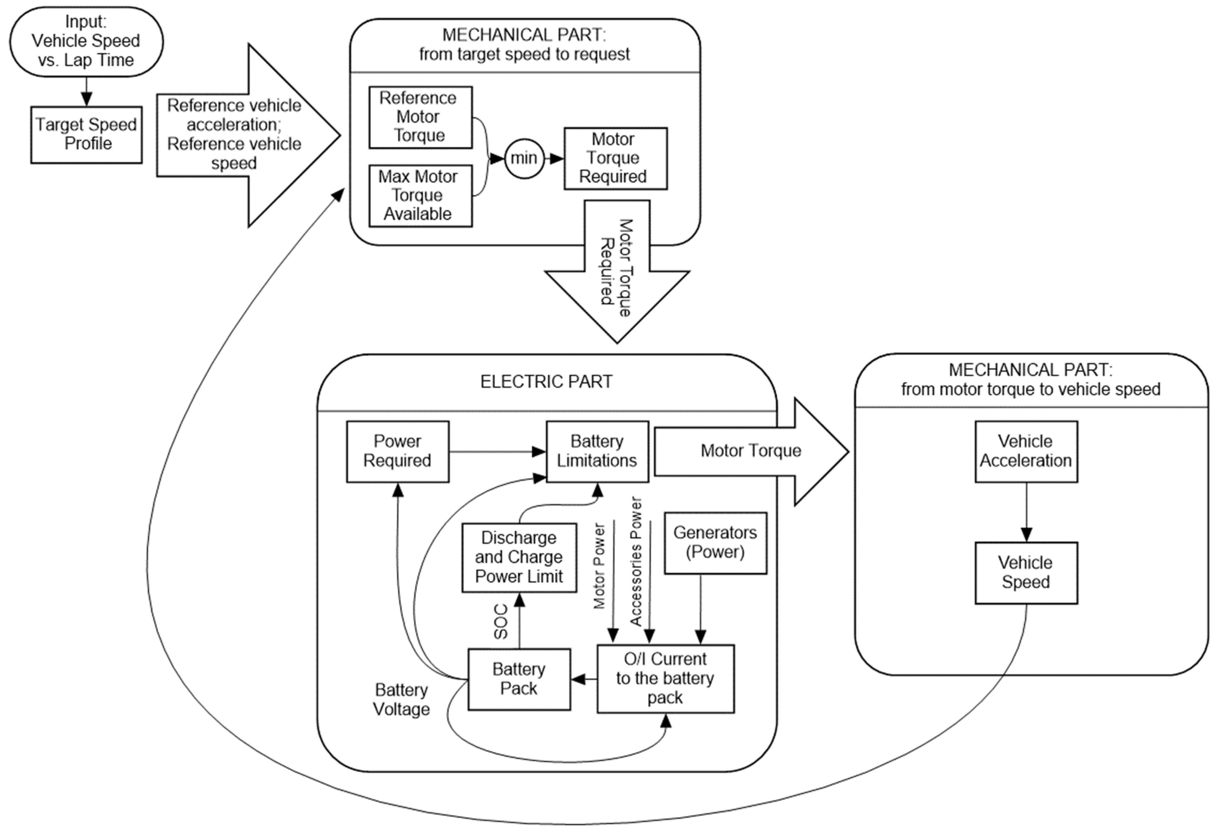
In this regard, following the same logic, the “Datasheet Battery” block has been reworked, to obtain one that works discreetly but following the same logic. The following paragraphs explain the operating logic of the entire program. Furthermore, Figure 1 shows a schematic illustration of the operation of the program.
2.1. Power Longitudinal Dynamics Modelling: From Target Speed to Request
Different speed profiles (different Laps) can be supplied as inputs to the model, once the profile to be followed is chosen, it is possible to filter it by defining a constant . The model considers as the input speed profile the moving average of values of the chosen speed profile. If you do not want to filter the profile, then simply set equal to 1.
The reference acceleration is obtained from the filtered speed profile using the following equation:
where is the target speed of the filtered speed profile, corresponding to the instant of calculation considered, is the actual vehicle speed of the instant of calculation preceding that considered and is the sample time of the simulation.
Considering the wheel radius and the reduction ratios, the model calculates the angular speeds of the wheels and the rotation speed of the electric motors, not taking into account any slippages, as in Equations (2)–(5).
where and are the angular speeds of the wheels, front and rear respectively, if the vehicle faithfully follows the imposed speed profile (and without slippages), while is the rolling radius of the front wheels and that of the rear wheels. is the rotation speed of the motor that acts on the front axle and is calculated only in the presence of this motor, otherwise it is set equal to zero, the same is true for which is the rotation speed of the motor that acts on the rear axle. and are respectively the overall reduction ratios of the differential and transmission on the wheel side (with respect to the gearbox) of the front and rear drive chain, while and are the reduction ratios of the reduction/gearbox front and rear.
In addition to the speed target, it is also possible to impose, for each Lap, a temperature profile of the battery pack, linked to the speed profile, obtained for example experimentally, by detecting the temperature of the pack on a real vehicle that travels the imposed speed profile. The space travelled by the vehicle is obtained by integrating the speed of the profile, if the vehicle faithfully follows the imposed cycle. The model, through the space travelled and using a one-dimensional Lookup Table, detects the altitude of the road at the point considered on the track. The slope of the road surface is obtained from the distance on the track and from the elevation profile, the slope is expressed as an angle in degrees (), as follows:
where is the difference between the altitude of the road at the point considered and the altitude of the point of the instant of calculation preceding that considered, while is the difference in distance traveled, between the current instant and the previous calculation instant, with the imposed speed profile.
In addition, if the vehicle is stationary, is imposed equal to that of the previous calculation instant. The calculation of the resistant forces (additional resistant or traction force due to the slope, rolling resistance force and aerodynamic resistance) is essential for the functioning of the model. The additional force given by the presence of the slope of the ground , positive if it acts as a resistant force, negative if it is in favour of acceleration, agrees with the speed vector and acts as a traction force) is considered through the following relationship:
is the unladen mass of the vehicle, is the driver’s mass (plus the mass of any passengers), is the mass of the fuel (considered constant during the simulation, in this first version of the model), necessary for powering the any generators.
The rolling resistance is considered constant with respect to the speed and calculated using Equation (8) as reported in [19] for nonzero speeds (and set zero for zero speed).
where is the static rolling resistance coefficient. The equation used to calculate the aerodynamic resistance is:
where is the air density, is the frontal area of the vehicle and is the longitudinal aerodynamic coefficient, considered constant. Therefore, in this first version of this model, no aerodynamic map has been considered yet, which would still be easy to implement.
In the “Reference Motor Torque” block, the motor torques required to follow the target speed profile are calculated. There is in output from this block also the traction force required by the wheels (including the contribution given by the inertia of the wheels themselves), necessary in different blocks to distinguish the cases in which a positive traction force is required (to accelerate or to partially overcome the resisting forces and decelerate less intensely compared to the absence of traction force) from cases in which a negative one is required (to have greater deceleration than that given only by the resisting forces).
Moreover, a balance of forces acting on the vehicle (in the centre of gravity) is carried out in order to identify the traction force necessary for the vehicle to travel with acceleration equal to that of reference, as in the following equation:
Adding the inertia contributions to the traction force, the total traction force at wheels must be recalculated. The inertia contributions, respectively of the front (11) and rear (12) wheels, are obtained through the following equations:
where the “2” coefficient is used to consider both wheels of the axle. and are the front and rear wheel inertia, respectively. The total traction force, including contributions due to the inertia of the wheels, is multiplied by if the electric motors are used for traction or by if the motors are used as generators to recharge the batteries during braking, to obtain the portion of traction force which must be guaranteed by the front motor. is the distribution of torque between the two electric motors (towards the front) in the case of the accelerator pedal pressed, is the distribution in the event that the brake pedal is pressed. Using these distribution values to divide the traction force between the two axles, an approximation is therefore being made. Obviously, if only the front electric motor is present on the vehicle, both distributions will have to be set equal to 1, vice versa, if the vehicle has only rear motor, both distributions will be null.
Finally, the motor torques required at the front and at the rear are calculated, using relationships (13) and (14), only if the motor is present, considering the contributions of input and output inertia to the gearbox, the motors inertia and a general transmission efficiency for transmission on each of the two axles.
where is equal to 1 in the case of motors that produce traction force and −1 in the case of motors that act as generators; and are the inertia coefficients of the moving mechanical parts in output respectively to the reducer/gearbox of the front and rear motor; and are the inertia coefficients of the moving mechanical parts in input respectively to the reducer/gearbox of the front and rear motor; is the inertia coefficient of the front electric motor, while of the rear one; and are the general efficiencies of the entire transmission, front and rear respectively.
Once the torques that the electric motors must supply or absorb in the case of braking (and in the absence of traditional brakes) have been obtained, it is necessary to compare them with the maximum available torques of the two motors to check whether the target mission can be met or not. The calculation of the maximum torque available for each motor (front or rear) is obviously carried out only if the motor in question is present on the vehicle, otherwise the maximum torque value is set at zero. To obtain the maximum torque of the motors, the angular speeds (in RPM) of the previous instant are considered. This is done as an approximation since the rotation speed of the motors at the instant considered is not yet known, the vehicle may in fact, due to limitations of the motors or batteries, fail to follow the target speed profile.
In the Simulink model the maximum motor torques are obtained thanks to the Lookup Tables containing information regarding the torque curves of the motors in the condition of maximum admission. The reference torque and the maximum available torque at the front are compared and the torque which will in turn be compared with the limits imposed by the battery pack is the lowest in modulus between the first two. The same approach can be adopted for the rear motor, for the calculation of . Alternatively, for one or both motors, it is possible to define a maximum torque for regenerative braking, which has a trend that grows linearly as a function of the time elapsed since the start of the braking and which then reaches a predefined maximum value (in module). This is what was done in the model, in the “Motor Torque Required” block.
Starting from the latter regenerative braking configuration, it is possible to return to the first described, simply by setting an absolute maximum braking torque equal to or greater than the maximum motor torque and an infinite angular coefficient for the equation of the straight line that binds time elapsed since start of braking and maximum regeneration torque at the instant considered. For the instant considered, it can now be considered that the rotation speed of the front and rear motor respectively, and , is equal to the reference rotation speed of the relative motor (closely related to the target speed profile) if there is no limitation given by the maximum performance of the motor in question. While, if the motor is unable to guarantee the torque required by the target, its rotation speed is approximated to that of the previous instant.
In the “Motor Torque Required” block, binary values (1 or 0) are also obtained as output depending on whether or not there are torque limitations due to the maximum performance of the motors, in the pressed accelerator condition () and in the braking condition (). The question is whether this limitation, respectively in the accelerator or brake pedal pressed phase, that is present on only one motor, is enough to trigger the variable or the unit value.
2.2. Power Electronics and BMS Modelling
Once the requests of the mechanical part have been defined, it is necessary to consider the electrical part to take into account any limitations given by the batteries and for the calculation of the power, current, voltage and SOC (State of Charge) parameters of the battery pack.
2.2.1. Battery Limitations
To know the power that the electric motors must request from the batteries (or the power that thanks to the motors recharge the batteries) it is necessary to know the powers lost due to the Joule effect due to the resistances of the electric cables that connect the motors and batteries themselves. Obviously, the connection cables are present only in the presence of the relative motor; therefore, in the absence of the latter the related resistance is considered null. The connection cables’ resistances between batteries and front and rear motor are calculated as follows:
where is the resistivity of copper (or any other material the electrical cables under consideration can be made), and are the total lengths of the connection cables of the front and rear motor respectively, and are the cross-sectional areas of the front and rear cables while is the diameter of the front cables and is the diameter of the rear cables.
Within the “Power Required” block, the total power required of the batteries by the electric motors (or that the motors could guarantee as input to the batteries) is calculated, instant by instant. This power is the result of an approximation as no voltage drop is considered as regards the resistance of cables and electric motors. In particular, the total power required is equal to the sum of the power required by the front motor and that required by the rear motor . The calculation of the latter two quantities is represented in Equations (17) and (18).
where and are worth 1 if the motors require energy from the batteries, -1 if the motors act as generators by sending energy to the battery pack. is the voltage of the battery pack and is calculated in the Simulink “Battery Pack” block of the model, and are the electrical efficiencies of the front and rear motor and they are obtained through a special block, which is present inside the “Power Required” block. The electrical efficiencies of the motors are calculated by the model only if the considered motor is present, otherwise the relative efficiency is set to zero. In particular, the efficiency of each motor is obtained thanks to a two-dimensional Lookup Table that receives in input the motor torque and motor speed and returns the efficiency.
To calculate the overall power input or output from the battery pack, it is also necessary to know the power supplied by the generators (if they are present). In this first version of the model, the possibility of integrating the vehicle with a number of generators that is zero or greater than zero was considered, where all the generators installed on the vehicle are identical and all have the same operation instant by instant.
Furthermore, no resistance of the connection cables between generators and batteries was considered, considered negligible. In particular, the generators have a constant rotation speed and a constant rated power output over time, unless the need to cut power due to the limitations imposed by the maximum performance of the battery pack.
In the “Generators” subassembly, the electrical efficiency of the single generator is obtained starting from the nominal power (, positive) of the single generator and its rotation speed , through a two-dimensional Lookup Table. Multiplying the efficiency by the rated power and by the number of generators gives the total maximum power value (, positive) that the generators can supply as input to the battery pack.
For the comparison of the balance of the power required, entering or leaving the battery pack, with the limitations of the pack itself, it is also necessary to consider the contribution of the power lost inside the cells due to their electrical resistance. First of all, the model, starting from the total power entering or leaving the battery pack and the voltage of the pack, calculates the theoretically required current if there are no limitations given by the batteries, as in Equation (19).
where is the total power consumed by the vehicle accessories, considered constant. A Lookup Table, which receives the temperature of the battery pack and the SOC at the input, returns the resistance of the single cell to the output.
Finally, the calculation of the total power of all cells, dissipated by Joule effect in the entire battery pack is:
where corresponds to the number of cells arranged in series inside the battery pack, while the number of those arranged in parallel. The power dissipated by the Joule effect thus obtained is relative to the case in the absence of limitations given by the maximum performance of the battery pack, but will be used, as an approximation, even in the cases in the presence of such limitations. In this way, in limited condition, an approximation of the power lost due to the internal resistance of the cells is made for excess. In the “Battery Limitations” block, the discharging and charging limitations of the batteries are considered. These limitations can be expressed as powers or as currents.
In particular, these limits are defined in function of the SOC of the pack and they are obtained in a dedicated subassembly which will be described later. The power balance shown below, in Equations (21) and (22), allows one to distinguish the case of discharge from that of recharging the batteries.
Discharge of the battery pack:
Charge of the battery pack:
Depending on whether the power balance mentioned above is positive (or null) or negative, one passes to considering an “if” subassembly or another in the Simulink model. In the case that the previous power balance is positive or null, the desired variables are the output from the “if” subassembly “Battery Discharge”. In this case, the generators can work by supplying the entire rated power as output, without the need for limitations.
In this block there are in turn two further “if” checks that divide the case in which there is no limitation imposed by the battery pack from that in which the power absorbed by the electric motors must be limited. The available power , which can be taken from the battery pack, is calculated as:
which is valid in the event that the discharge limit of the battery pack is supplied as a limit current (positive, ), if it is expressed as a power (positive, ) the previous relationship must be reconstructed as follows:
where is simply a constant power that is used to keep within the discharge and charge limits with a defined tolerance, equal to the value of this constant and is the “real” power supplied to the batteries by the generators, which in case of discharge is equal to the maximum power , without the need for any limitation. The power to be taken from the battery pack consists of the sum of the power absorbed by the vehicle accessories (, considered constant) and the total power required by the electric motors . By subtracting the contribution of these two powers from the maximum available, it is therefore possible to ascertain whether this is actually available and therefore no limitation is necessary or vice versa (i.e., if the result of this subtraction is positive or negative).
In the event that there are no limitations given by the battery pack being discharged, the required quantities will actually be the “real” ones of the vehicle, at the instant considered (remembering that the limitations of maximum drive torque have already been considered), and they will be taken as output from the first “if” block.
A binary control variable is also defined, , defined in this case equal to 0, defined instead equal to 1 in the condition of limitation of the motors during traction due to the maximum performance of the batteries. The calculations are carried out in the second “if” block if it is necessary to impose limitations during the discharge phase. In the case with limitation in the discharge phase, if the available power is not enough even to power the accessories, obviously the electric motors will be turned off and it is necessary to define the variable to keep track of the amount of power missing for the power supply of the accessories. is defined equal to the difference between available power and power that should be absorbed by the accessories. On the other hand, if after the part of available power supplied to the accessories is considered, a part of power remains available; the latter will be used to power the electric motors.
In the presence of both motors, this power will be divided between front and rear through the distribution constant . Below are the calculations of the front drive torque , in Equation (25), and rear , in Equation (27).
For the calculation of both motors torques, it is taken into account the resistance of the cables (but the relative voltage drop is neglected), the electrical efficiency of the motors ( and , obtained by means of the Lookup Table, starting from the efficiency map of the motors) and the equality of the instantaneous rotation speed of the motor ( and ) is set as an approximation to the rotation speed relative to the previous instant of calculation ( and ) as show in the Equations (26) and (28).
The foregoing is valid in the event that the electric motors must absorb power from the battery pack, but it could fall into the limit case in which the motors act as generators (), but the power absorbed by the accessories is still sufficient to ensure that the batteries are being discharged. In this case, no limitation is required for the motors torque and the will be calculated as follows (29).
The control variable is defined for both motors and the output variable to the “if” block will be equal to 1 if that relating to at least one motor is unitary (i.e., if at least one of the motors is limited by the maximum performance of the battery pack), equal to zero vice versa. If a motor (front or rear) is not present on the vehicle in question, all the relevant quantities are defined as null, including the variable. In case that the battery pack is in a recharging condition, the desired variables are output from the “Battery Charge” “if” subassembly, contained in the “Battery Limitations” block. In the “Battery Charge” block there are in turn two further “if” blocks that divide the case in which there is no limitation imposed by the battery pack from that in which it is necessary to implement limitations. The maximum power that the battery pack can absorb is calculated using the following equation:
Equation (30) is valid if the discharge limit of the battery pack is supplied as a limit current (negative, ), if it is expressed as a power (always negative, ) the previous relationship must be reconstructed as follows:
It is therefore possible to understand if it is necessary to make limitations or not, considering the power contributions of generators and electric motors. The outputs are obtained from the “if” subassembly relating to the absence of limitations if the inequality (32) is valid, from the “if” subassembly relating to the presence of limitations vice versa.
When no limitation is required during the battery discharge, the system variables are considered equal to those resulting from the comparison with the maximum performance of the electric motors. binary control variable is also defined, null in the absence of limitations of the electric motors when braking (and also even if the motors participate in traction), set equal to 1 in the case of motor limitation during regenerative braking, due to battery limitations. is instead a binary quantity useful for checking that the generators have been limited (when it is equal to 1) or less (equal to zero).
The “if” subassembly relating to the presence of current limitations is in turn divided into two “if” subassembly, “Without Motor Power Restrictions” and “With Regenerative Braking Restriction”. The model recovers the variables of interest from the first “if” block if the maximum that the battery can absorb (negative) is less than or equal to the required power (input or output to the battery pack) from the motors, vice versa from the second “if” subassembly. The logic adopted is to limit the generators first, so as to be able to guarantee the regenerative braking of the motors within the limits (so as to be able to exploit the traditional brakes of the vehicle to a minimum) and only in case of need for further limitation also limit the electric motors. If it is sufficient to implement the limitation to the generators only, the only new quantity to be calculated is precisely the “real” power that the generators supply to the battery input , equal to the difference between the total power of the motors and the maximum absorbable power battery . The difference has been structured in this way to ensure that the power of the generators is positive. If it is also necessary to limit the power of the electric motors, the generators will be turned off and all the power supplied as input to the battery will be guaranteed by the electric motors . In this case, the control variables will assume the following binary values, represented in Equations (33) and (34).
The total power supplied by the motors is divided between the front and the rear by means of the distribution constant . The new quantities of the system are obtained by means of the Equations from (35) to (38).
Again, the motors’ efficiencies are obtained by means of Lookup Tables and the voltage drops caused by the resistances of the electric cables are neglected. Furthermore, the rotation speed of the motors is approximated to that of the previous calculation instant. This part of the Simulink model, which includes the limitations of the battery pack, represents part modelling of the BMS. The logic of the BMS is strongly linked to the type of battery and the strategies adopted by the vehicle manufacturer. For this reason, these logics can vary greatly depending on the type of vehicle and its mission.
2.2.2. Battery Parameters
Once the requests for electric motors and generators have been defined, after applying the necessary limitations, it is necessary to know the input or output current to the battery pack. The calculation of the current is very simple, and it is represented by the equation number (39).
where the total battery power deriving from the electric motors is the sum of the front contribution and rear contribution .
Considering the current passing through the battery pack, relative to the previous calculation instant with respect to the one considered, it is possible to obtain all the battery values of interest, including the voltage of the pack, used for the calculations inside the blocks previously exposed.
In the model, the thermal balances are not taken into account, the temperature can therefore be assumed constant or supplied as input starting from experimental values measured according to the target speed profile.
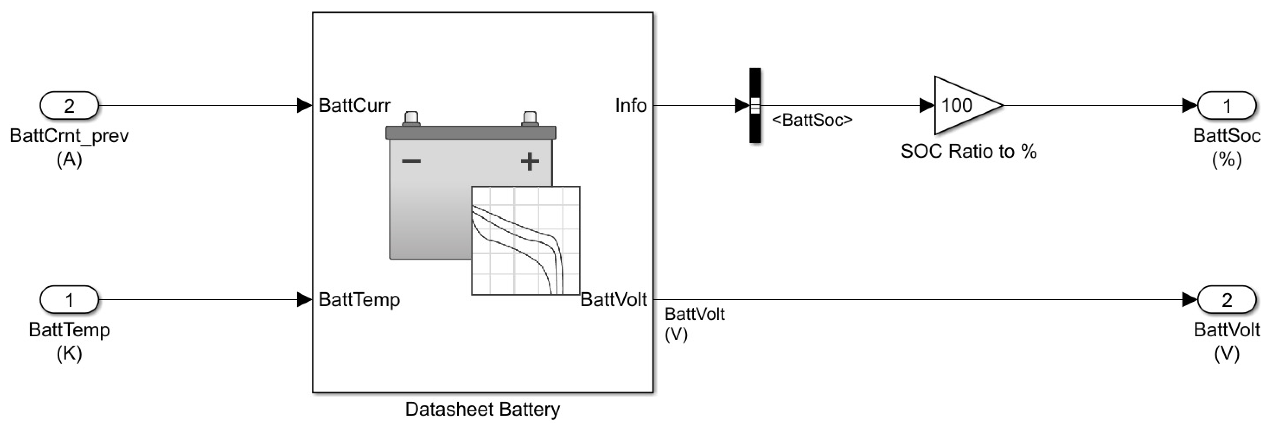
Furthermore, by multiplying the current and voltage between them, it is possible to obtain the incoming (negative) or outgoing (positive) power from the battery pack, starting from the current of the previous calculation instant () and the instantaneous temperature of the battery pack, it is possible, through the “Datasheet Battery” (Figure 2) block of the Simulink library, to obtain battery state of charge and voltage () of the pack. The battery block of the Simulink library is an internal resistance battery model [10] and it is easily replicable for its discreet use if there is the need to perform this type of simulation.
Finally, to conclude the discussion concerning the electrical part of the model, the origin of the discharge and charge limits of the battery pack, obtained starting from the state of charge of the battery pack, is described. Both limits are obtained using Lookup Tables which contain information about the link between SOC and limit in discharge and the link between SOC and limit in charge.
2.3. Power Longitudinal Dynamics Modelling: From Motor Torque to Vehicle Speed
Once the limitations given by the electrical part have also been considered, it is necessary to define how the vehicle responds to the set speed target, faithfully following it or departing from it due to the limitations.
In the “Vehicle Acceleration” block, a balance of forces (see Equation (40)) is carried out again, as in the case of the “Reference Motor Torque” block, but this time to find the “real” acceleration () of the vehicle, starting from the limited motors torques (if necessary).
Thanks to the motor torque and the rotation speed of each of the electric motors, it is possible to obtain the front and rear traction force provided by the motors (positive if it is really a traction force, negative in the case of regenerative braking).
If there is an electric motor that acts on the front axle, the related traction force is calculated as in (41), while it is imposed null in the absence of this motor. It is the same with regards to the electric motor that acts on the rear axle (42).
with for , otherwise .
with for , otherwise .
The contributions given by the inertia of the front and rear wheels are calculated as follows using Equations from (43) to (46).
If the front electric motor is present:
If the front electric motor is absent:
If the rear electric motor is present:
If a rear electric motor is not included:
The braking force of traditional brakes must be that necessary to integrate regenerative braking, if necessary, to allow the vehicle to follow the speed target when braking, unless there is any limitation given by the maximum permissible braking of the braking system. In the “Traditional Brakes” block, located inside the “Vehicle Acceleration” assembly, the balance of forces reported in (47) is carried out to obtain the braking force required (, defined positive) from the brake system.
This force must be compared with the maximum force that can be generated by the braking system (, defined positive). The effective will be equal to the smaller of the two. The following equation shows the calculation of :
where is the maximum pressure that can be generated inside the master cylinder of the brake system; represents the pressure portion, compared to that of the master cylinder, which acts on the front brakes; and are the total action areas of the brake pistons of the front and rear callipers respectively; and are the dynamic coefficients of friction between brake pads and brake callipers, front and rear; and are respectively the average radii of application of the braking force on the front and rear discs. In the “Traditional Brakes” block a further control parameter called is defined, which is set to 1 if there is a limitation of traditional braking or equal to 0 instead.
The aerodynamic drag force is equal to calculated previously on the basis of the target speed if in the instant considered there are no limitations to the motors caused by the maximum performance of the motors themselves or by the maximum performance of the battery pack and if there is no limitation of the traditional brakes. Otherwise, is calculated using, as an approximation, the vehicle speed of the instant of calculation preceding the one considered. To avoid incurring approximation errors during the calculations, the “real” vehicle acceleration output from block “Vehicle Acceleration” is that calculated using Equation (40) if there are limitations that lead to the failure to follow the target speed, otherwise is defined equal to .
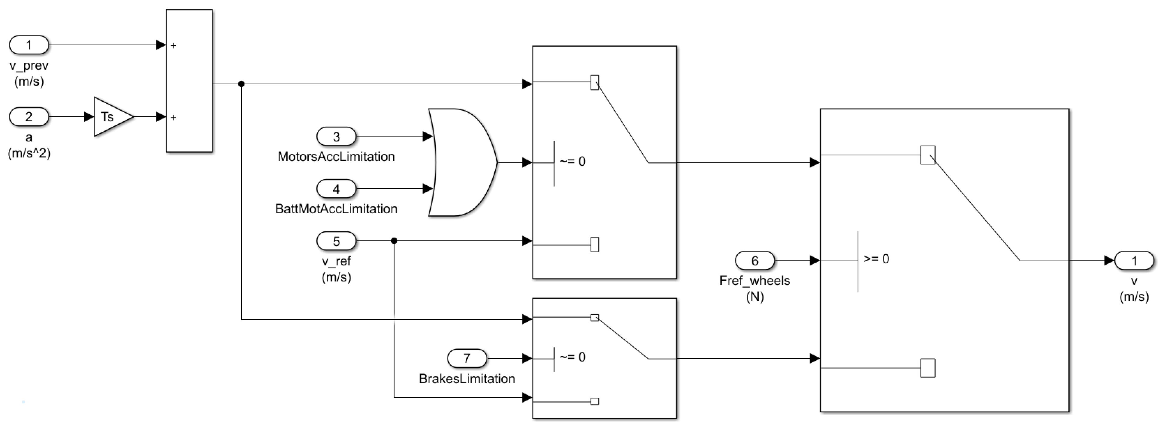
A further block relating to the mechanical part with limitations is the one called “Vehicle Speed”, which outputs the “real” vehicle speed. The logical scheme adopted to obtain the “real” speed followed instant by instant by the vehicle is shown in Figure 3. As can be seen, appropriate measures have been taken to prevent the propagation of the approximation errors, inevitable during the calculations and due to different approximations adopted in the model. The sign of the variable is used to distinguish the case of the accelerator pedal pressed from the case of the brake pedal pressed.
For the calculation of the speed (), where necessary, a uniformly accelerated motion between one instant of calculation of the simulation and the next was considered, see Equation (49).
Finally, from the speed it is also possible to obtain the space travelled by the vehicle () during the execution of the actual driving cycle, once again considering motion uniformly accelerated between two successive calculation step, as in the following equation:
where is the space covered by the vehicle from the start of the simulation until the calculation step preceding the one considered.
2.4. Outputs
Once the simulation is completed, all variables will be saved in MATLAB workspace. Therefore, the outputs are completely “customizable by the user” based on the variables he wants to analyse. In Section 4, an example layout will be shown for the outputs with the most relevant quantities.
3. Graphic User Interface
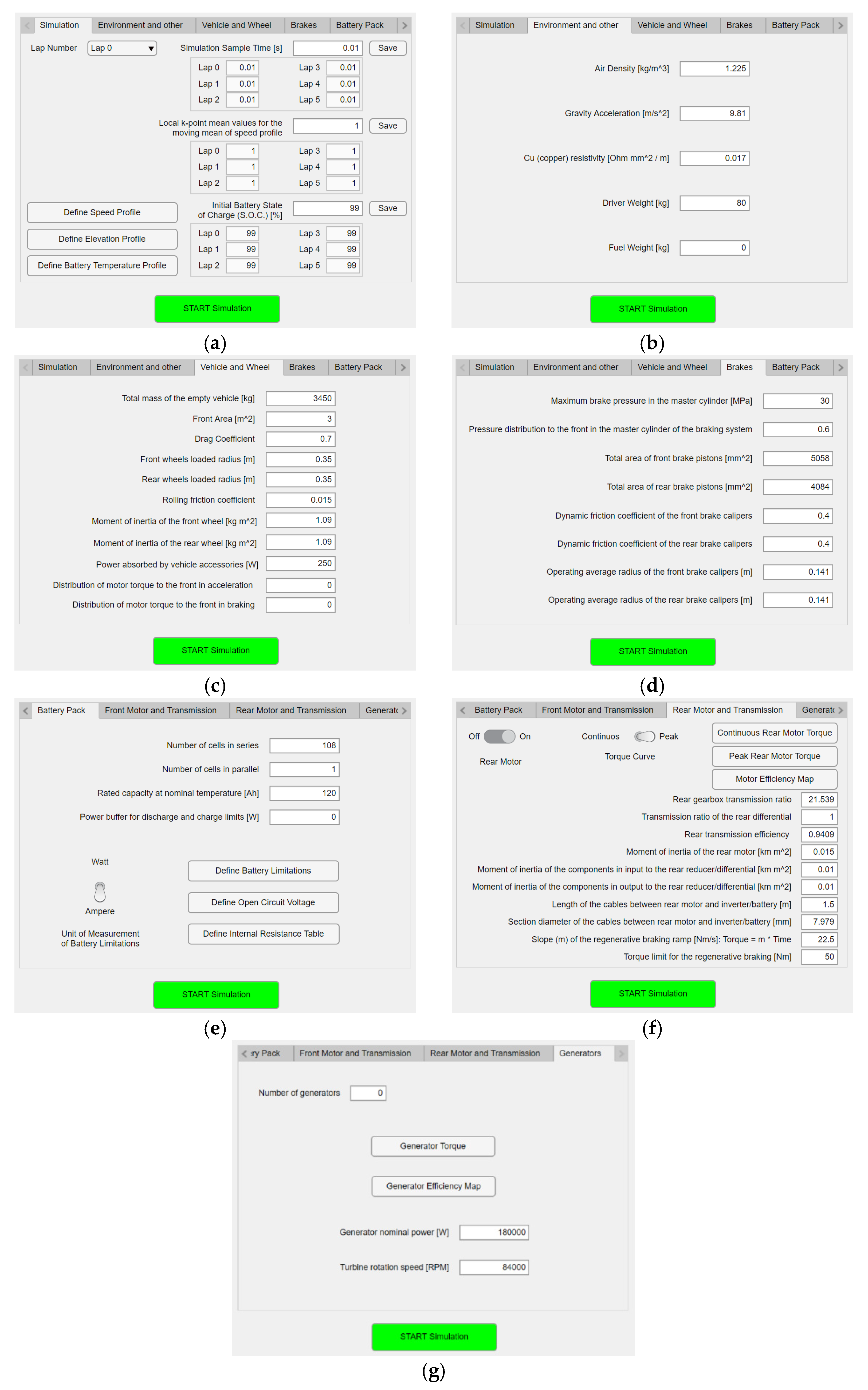
For easier and simpler management of the Simulink model, a graphic user interface has been created, using the “App Designer” tool of MATLAB, which allows for the control and modification of all the inputs of the model and starts the simulation. In particular, it is possible to save, for a specific vehicle, six different simulations (from Lap 0 to Lap 5), relating to six different speed profiles, each filtered through the average of elements (with that can differ between a Lap and the other), with relative altimetric profiles, with fixed sample time of simulation and initial state of charge of the battery pack (Figure 4a).
Furthermore, it is possible to define all the environmental parameters and other parameters such as the driver’s weight and the weight of fuel on board, necessary to power any generators (Figure 4b). It is then possible to define as input all the parameters relating to the vehicle in general, the wheels and the braking system (Figure 4c,d). The APP also allows you to set all the parameters relating to the batteries, with the option of choosing to enter information regarding the charging and discharging limitations in Ampere or Watt, and the two electric motors, front and rear (Figure 4e,f). For each motor it is possible to define both the continuous and peak torque curve and choose which one to use during the simulation, as can be seen from Figure 4f. Therefore, there is still no implementation in the model of an automatic management of the peak torque for the maximum allowed time and then an automatic transition to the maximum continuous torque. Finally, it is possible to modify all the input parameters concerning any generators in parallel installed on the vehicle (Figure 4g). Using the “START Simulation” button, simulation is started, and the graphic results are shown. The information regarding the simulation and some variables of the simulation itself are also automatically saved in the workspace, such as the electric motors torques, the voltage and current of the battery pack, etc. It is however possible to save any other quantity and display any other graph as long as they represent variables calculated in some branch of the Simulink model described in Section 2, entitled “Simulation Tool”.
4. Model Validation
The validation of the model was carried out by comparing two borderline cases: a low-performance vehicle in terms of traction performance and a very high-performance hypercar. In the first case the validation was carried out through the comparison between model results and experimental data acquired through the VCU (Vehicle Control Unit) installed on a vehicle in the prototyping phase. In the second case the validation was carried out through the comparison between TEST and PROPS [8] results.
Furthermore, the driving missions of the two vehicles are also very different, in the first case an urban driving context is considered, in the second case the driving mission is of the Motorsport type, on the track.
4.1. Validation with Low Performance Vehicle
For the validation of the model under conditions of common driving cycles used in the public roads, the results of the model (obtained by setting the appropriate data concerning the specific vehicle) were compared with the data obtained experimentally from the VCU (Vehicle Control Unit) of a waste collection vehicle in the prototyping phase.
4.1.1. Powertrain
The prototype being simulated has a purely electric powertrain and it is a rear-wheel drive, with a single electric motor powered by a lithium battery pack. The configuration of this vehicle does not include any type of generator that recharges the battery pack, the only charging function in the simulation is the use of the electric motor as a generator during regenerative braking.
In particular, when the accelerator is released there is a regenerative torque which increases linearly with the time from the beginning of the release up to a maximum value, later this value remain constant until the accelerator pedal is pressed. In the same way, regenerative braking also intervenes with the brake pedal pressed.
4.1.2. Traction Motor
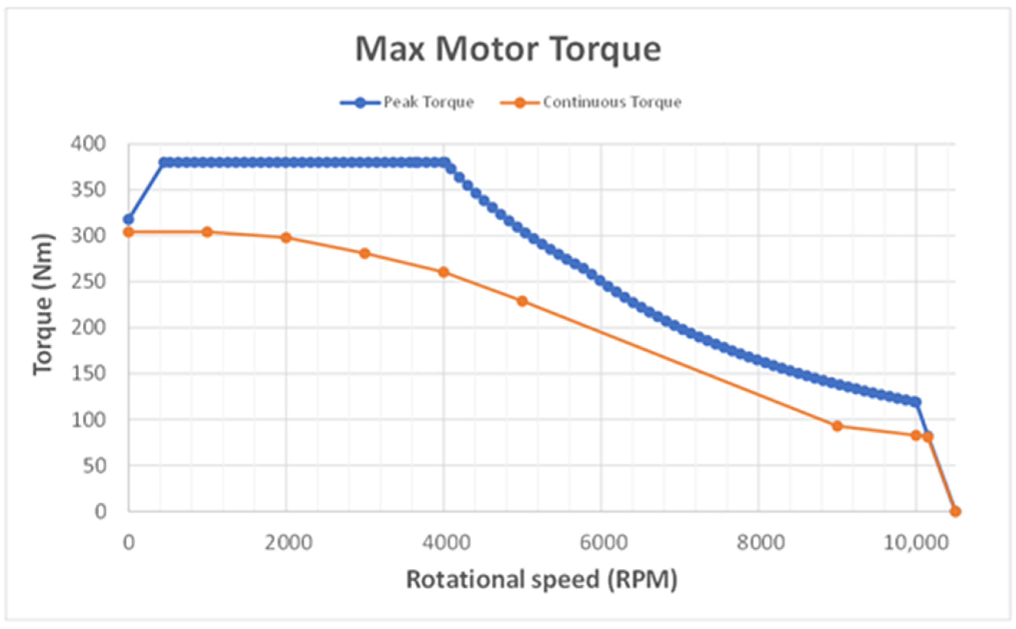
The electric motor is three-phase with an assembly mass of 57.2 kg and a rotational inertia of 0.086 kg·m2. It is characterized by the peak and continuous torque curves shown in Figure 5. In particular, the maximum peak torque is 380 Nm, while the maximum continuous torque is 304.3 Nm.
4.1.3. Battery Pack
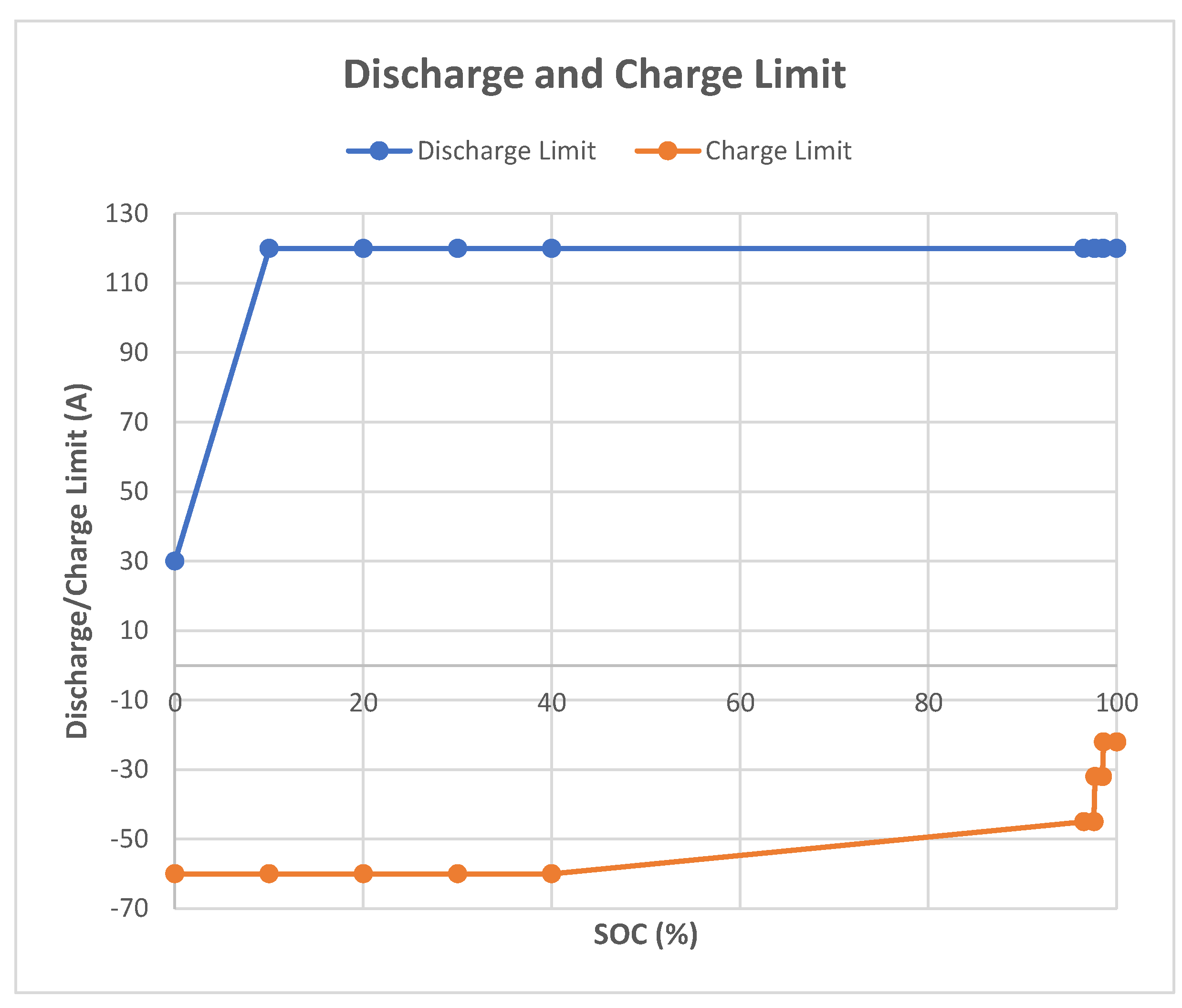
The battery pack consists of 108 lithium cells arranged in series which give it a maximum nominal capacity of 120 Ah. Regarding the outgoing current (positive) and incoming current (negative), the battery pack has the limits shown in Figure 6, depending on the state of charge.
The open circuit voltage (OCV) and the internal resistance (RES) of the battery pack were considered constant, in fact the average temperature of the cells detected by the BMS is constant during the test and the SOC does not vary significantly. OCV and RES were derived from the experimental data and their values are represented in the Table 1, together with the other main data of the vehicle.
4.1.4. Data Acquisition System
The data needed for comparison with the program results was acquired through the vehicle control unit. The VCU installed on the prototype is an Ecotrons VCU, model EV2274A. A speed profile followed by the vehicle was used for the simulation and the corresponding motor torque and battery SOC, current, voltage and power were used for the comparison with the model results.
4.1.5. Target Speed Profile
The mission of the waste collection vehicle object of this model validation is a public road driving cycle. The target speed profile for validation was obtained thanks to road tests carried out with a vehicle prototype, acquiring all the data of interest from the VCU. Table 2 shows the main data of the target speed profile considered.
4.1.6. Comparison between Model Results and Experimental Data
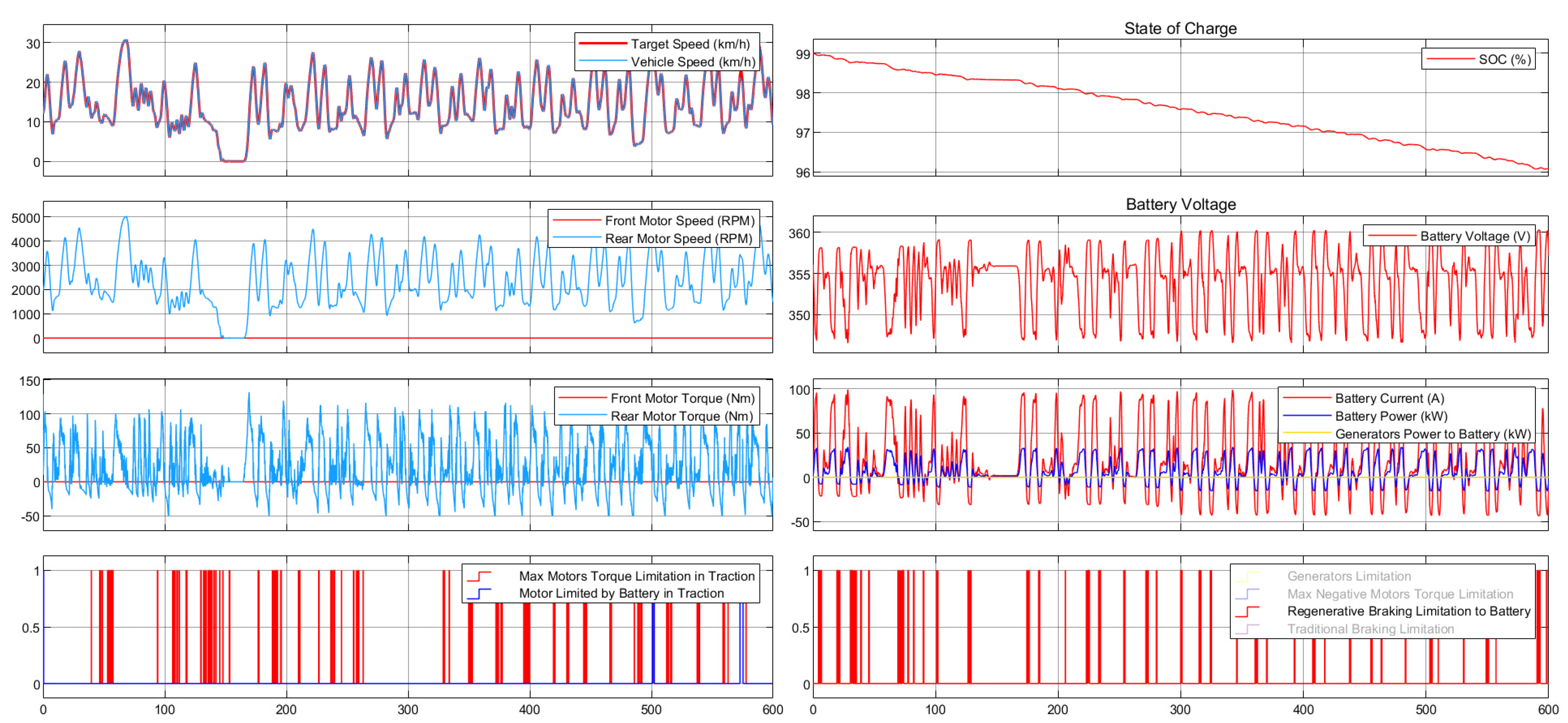
Figure 7 shows a general overview of the results screen. The most important model results for validation will be analysed in more detail later.
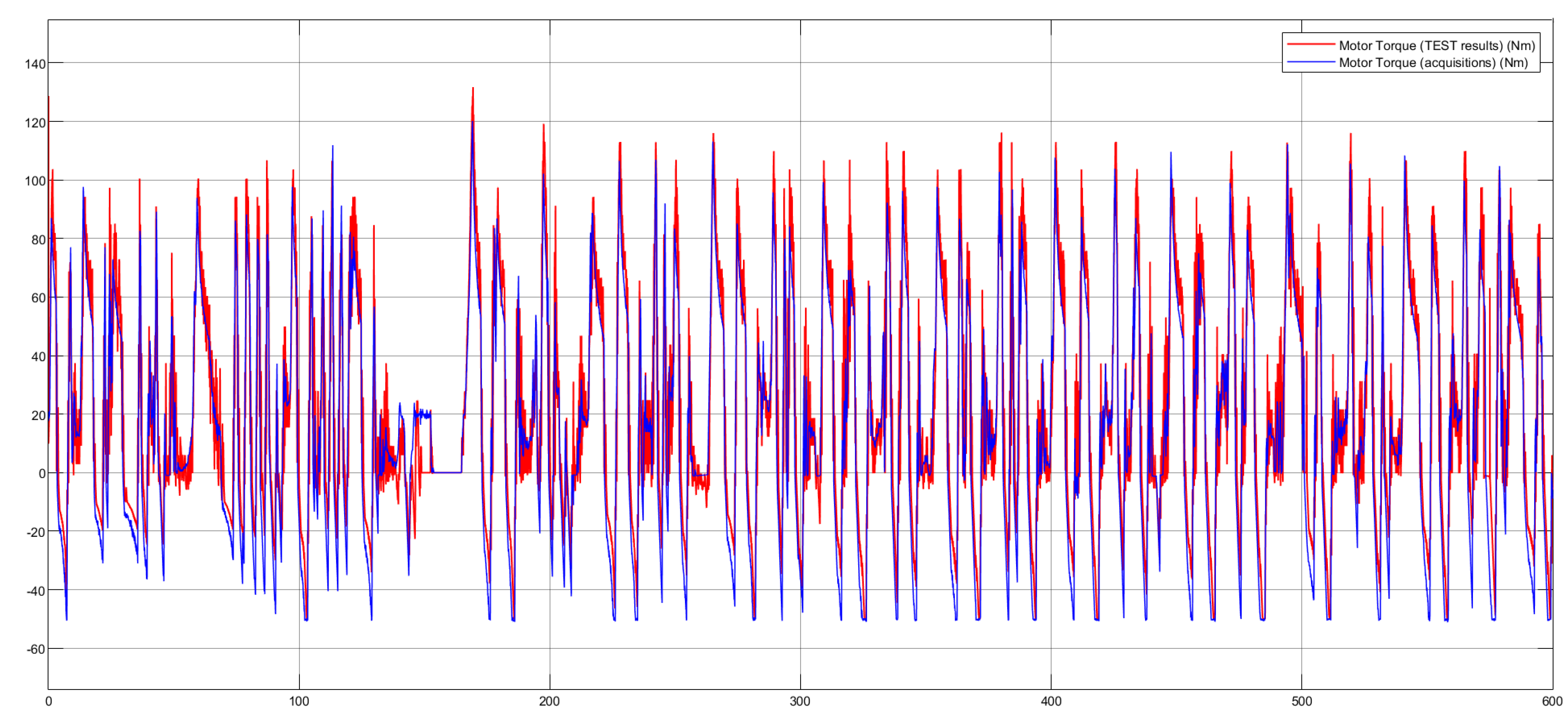
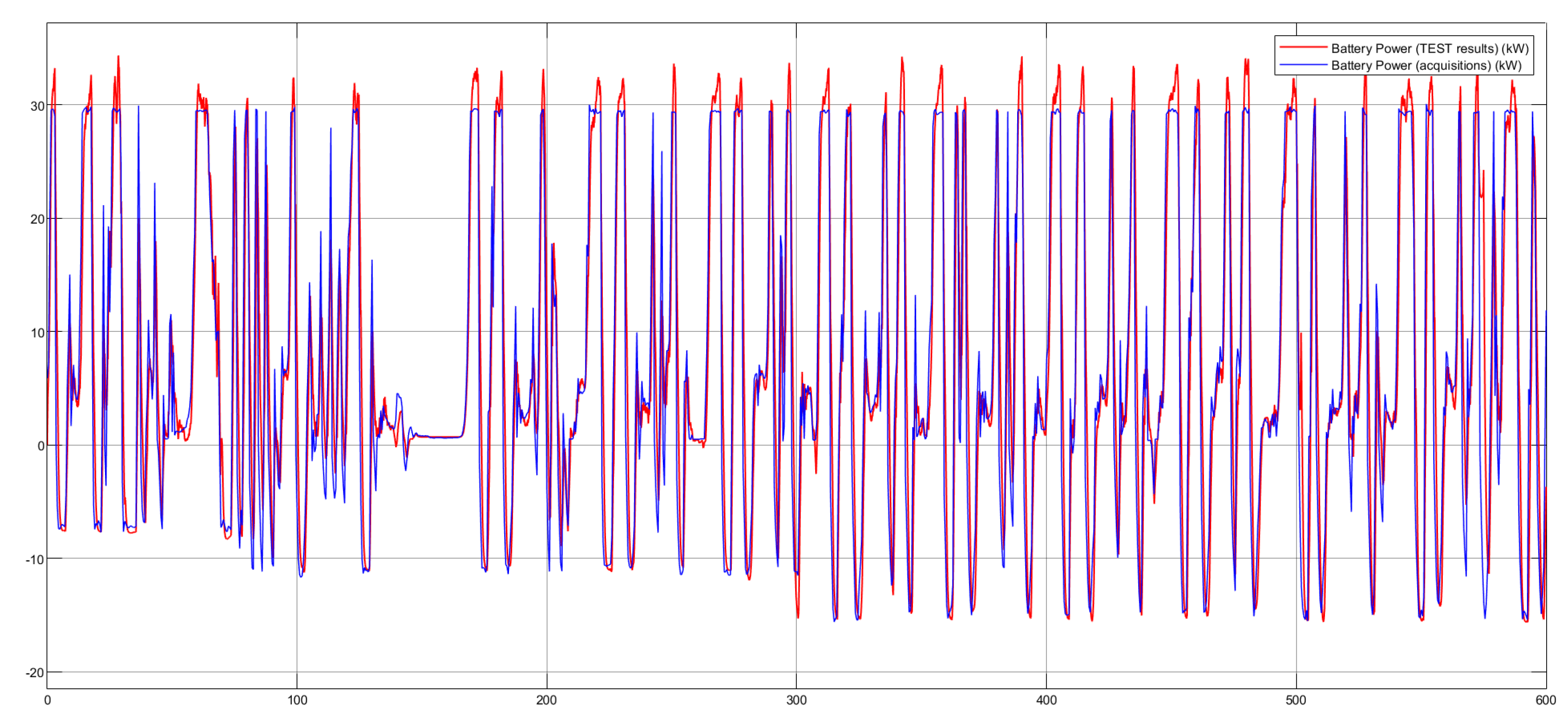
The mechanical part of the model works well, as can be seen in Figure 8, which shows the comparison between the motor torque obtained from the model and the experimental motor torque.
The motor torque values obtained in output from the model are much noisier than the real torque values (acquired through the VCU). This is because the model does not consider transients; it calculates the quantities considering only the calculation instant in question (and the previous). The quantities of the model (such as the motor torque and the battery power) can therefore theoretically vary instantly abruptly.
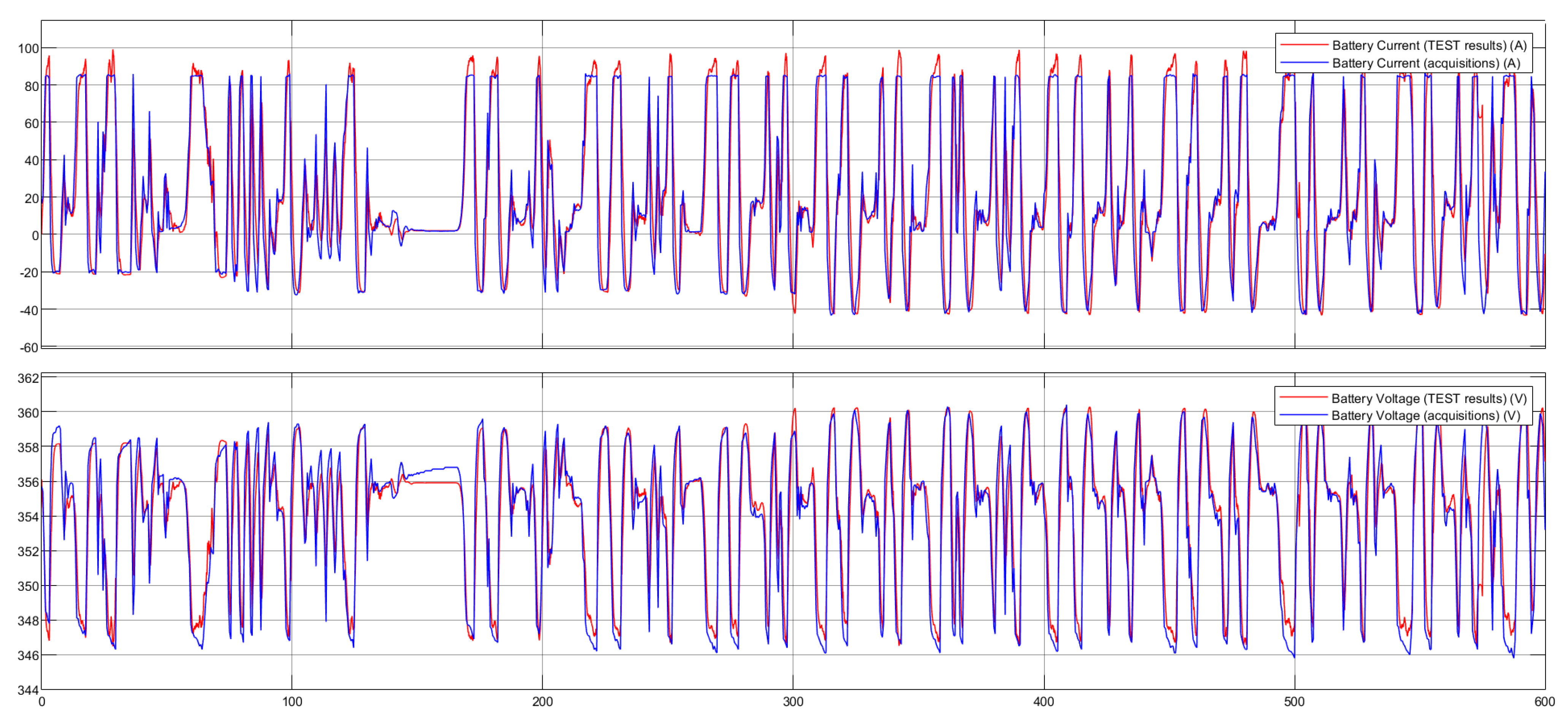
For the electrical part of the model, it was necessary to calibrate the power required at the battery terminals, inserting two efficiencies, one for the discharge case and one for the charging case. These efficiencies could represent the initially neglected power dissipations in the inverters and in the BMS. Figure 9 shows the comparison between the power obtained experimentally and the battery power resulting of the calibrated model while Figure 10 shows the comparison regarding current and voltage of the battery pack.
The differences between battery current and voltage obtained through simulation and acquired by the BMS (real data) are partly due to the fact that the battery model (“Datasheet Battery”) does not consider transients. For example, between 100 and 200 seconds elapsed from the start of the test there are about 20 seconds in which the vehicle is stationary, the current outgoing from the battery pack is constant and equal to about 2 Amperes and the battery voltage in output from the model is constant and equal to about 356 Volts. The current is not zero since, even when the vehicle is stationary, the auxiliaries must be powered. In real data it is possible to observe that the battery voltage does not remain constant in these 20 seconds but gradually increases. This is an effect due to the transient, in fact the Open Circuit Voltage (OCV) of a battery pack at rest tends to increase until it stabilizes at a maximum value.
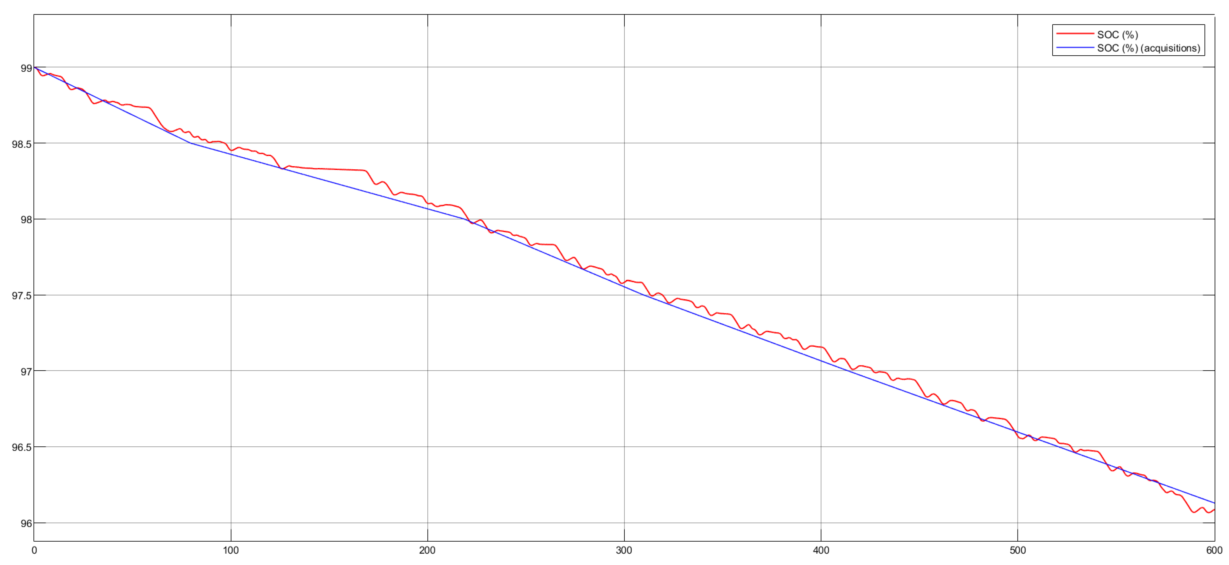
Finally, the Figure 11 shows the comparison between the SOC obtained experimentally thanks to the BMS (Battery Management System) and the SOC resulting of the model. The SOC acquired through the VCU has a sensitivity of only 0.5% of variation, for this reason the SOC curve represented in the graph of the Figure 11 is piecewise linear, it was obtained by joining the points where the BMS has detected a change in SOC. To obtain the performance indices of the model (shown in Table 3), the error was obtained (calculated as the difference between the output parameter of the model and the parameter acquired through the VCU prototype) and its mean and standard deviation were calculated. The mean and the standard deviation (std) were also calculated for the absolute value (abs) of the error. The differences between the model results and the experimental data can be considered negligible; the model is thus validated.
4.2. Validation with High-Performance Hypercar
For the validation of the model with data and operation typical of a high-performance vehicle, the data of an ultra-high performance hypercar, which is in the design stage, were considered. The speed profile adopted was obtained through a best lap time test of the car in question on the Nürburgring circuit, implemented in VI-CarRealTime (VI-Grade). As already mentioned in Section 1, the results from the TEST model were compared with those coming from a different simulation tool (PROPS) as reported in [8] and the comparison allowed for the performance of a correct calibration of the program.
4.2.1. Powertrain
The simulated hypercar is an APU (Auxiliary Power Unit) hybrid car, equipped with two electric motors, one acting on the front axle and one acting on the rear axle. Electric motors are powered by a lithium battery pack and they provide (or absorb) the same power at all times. Two generators are also installed on the vehicle, represented by two turbines powered by a liquid fuel, in particular by petrol. These generators are used to recharge the battery pack at constant power, unless limited by the battery pack itself. The generators are therefore always active while driving, rotating at constant speed, and their power is cut where the maximum charging limits (depending on the SOC) of the battery pack require it.
4.2.2. Traction Motor
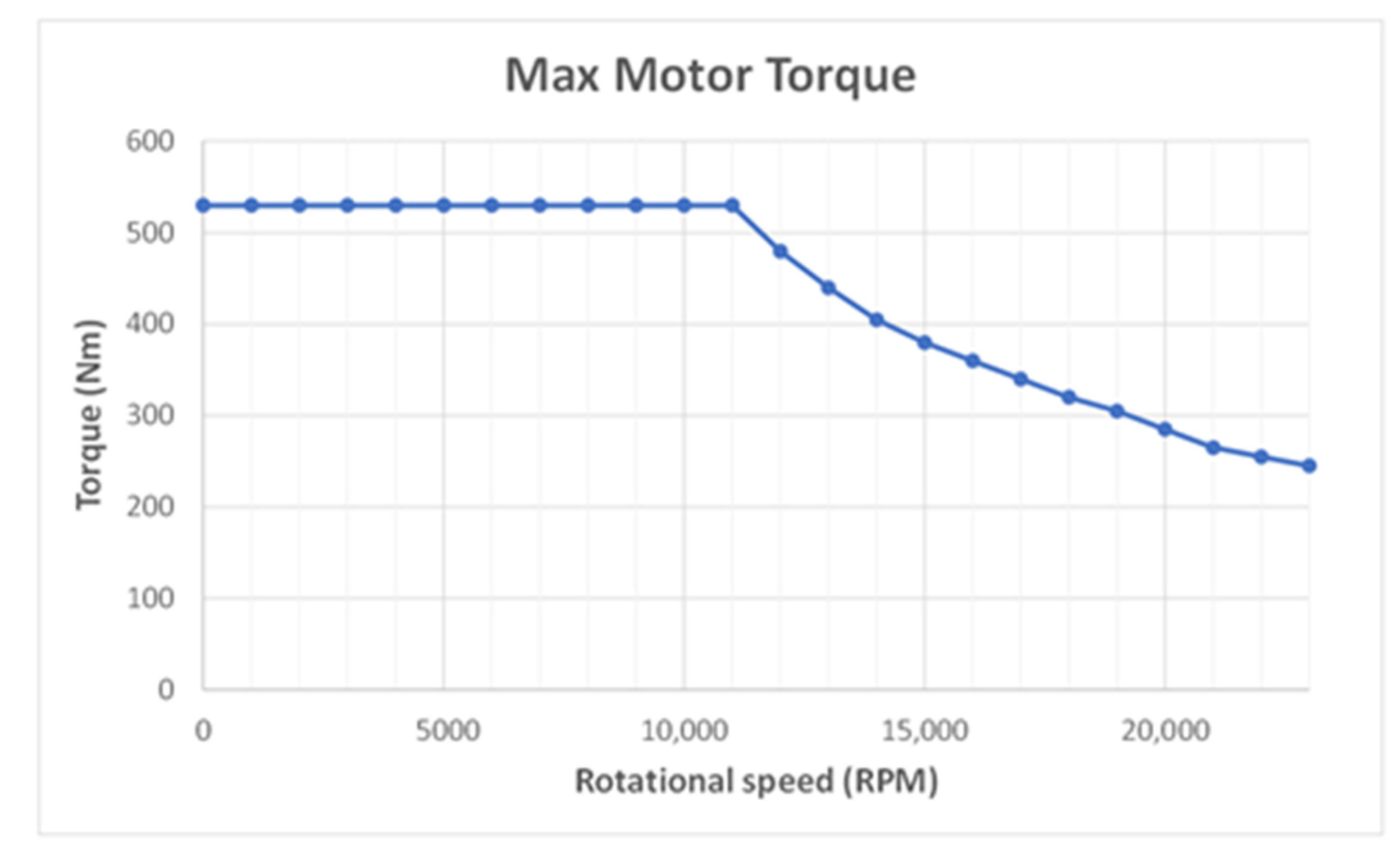
The two electric motors of the car are identical, and they present the torque curve in maximum admission condition represented in Figure 12. The maximum torque of the motors is equal to 530 Nm and the rotation speed is limited to 23,000 RPM.
4.2.3. Battery Pack
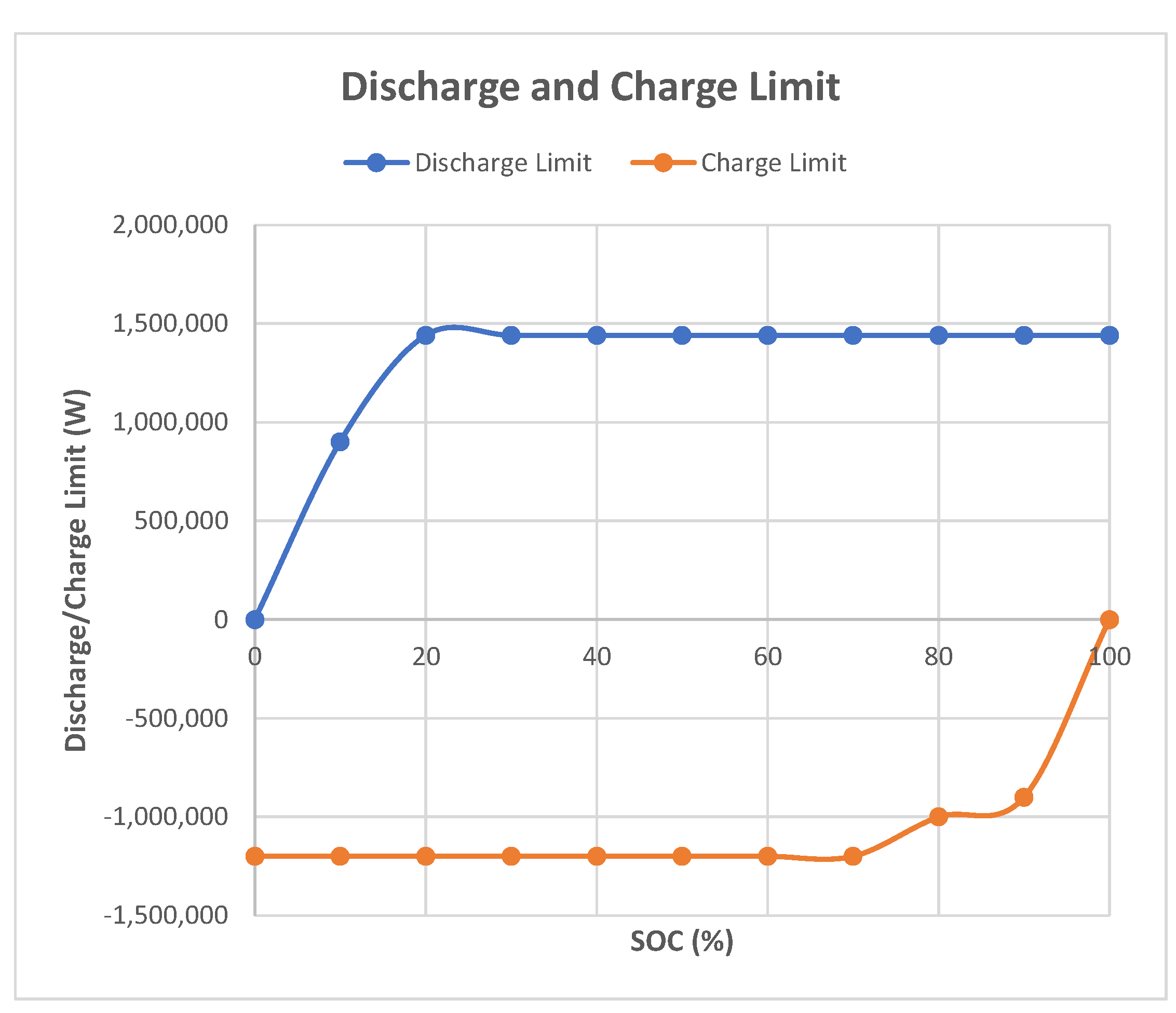
The battery pack configuration consists of 226 cells in series and 4 in parallel, for a total of 904 cells, with a maximum capacity of 6.55 Ah. The operating temperature of the cells must remain around 60 °C and the maximum charge and discharge limits must not be exceeded, limits that depend on the SOC and they are represented in the Figure 13, where the positive powers refer to the discharge and the negative ones to the charge of the battery pack.
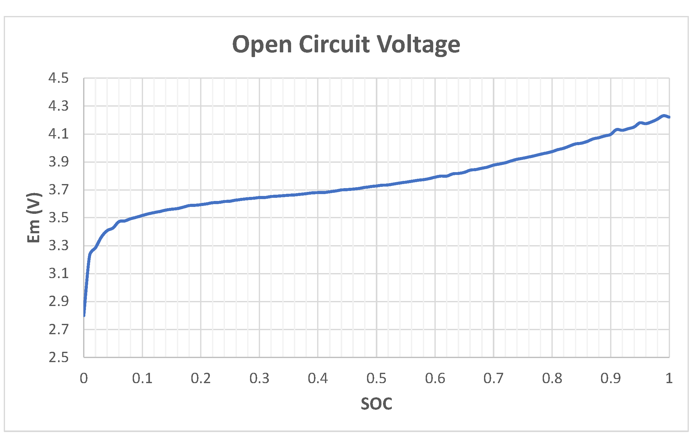
In order not to exceed the maximum limits it was defined to remain within the limits with a buffer of 1500 Watts. From Figure 14 it is possible to observe how the Open Circuit Voltage (OCV) varies according to the SOC of the battery pack. The internal resistance of each cell varies as a function of SOC and temperature, as can be seen from Table 4. Furthermore, in Table 5 main vehicle data is reported.
4.2.4. Generators
The vehicle in question is equipped with two generators for recharging the battery pack. Each generator can deliver a nominal power of 180 kW and a maximum torque of 530 Nm, thanks to the relative turbine which rotates at a constant speed of 84 thousand RPM. These values are shown in Table 5, which summarizes the main quantities of interest of the hypercar used for the validation of the model.
4.2.5. Target Speed Profile
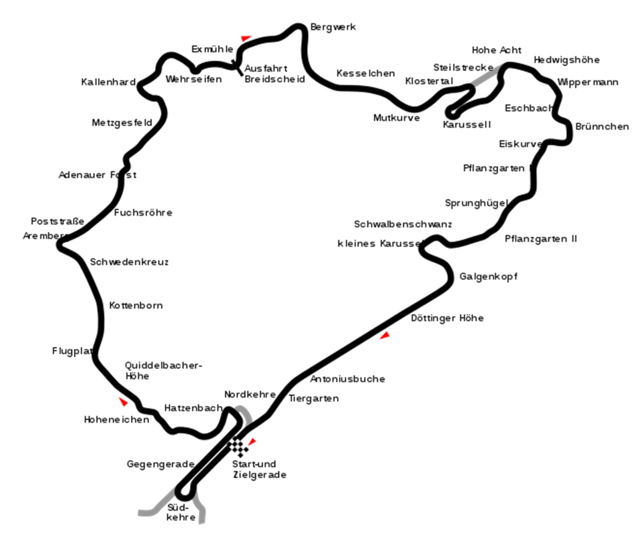
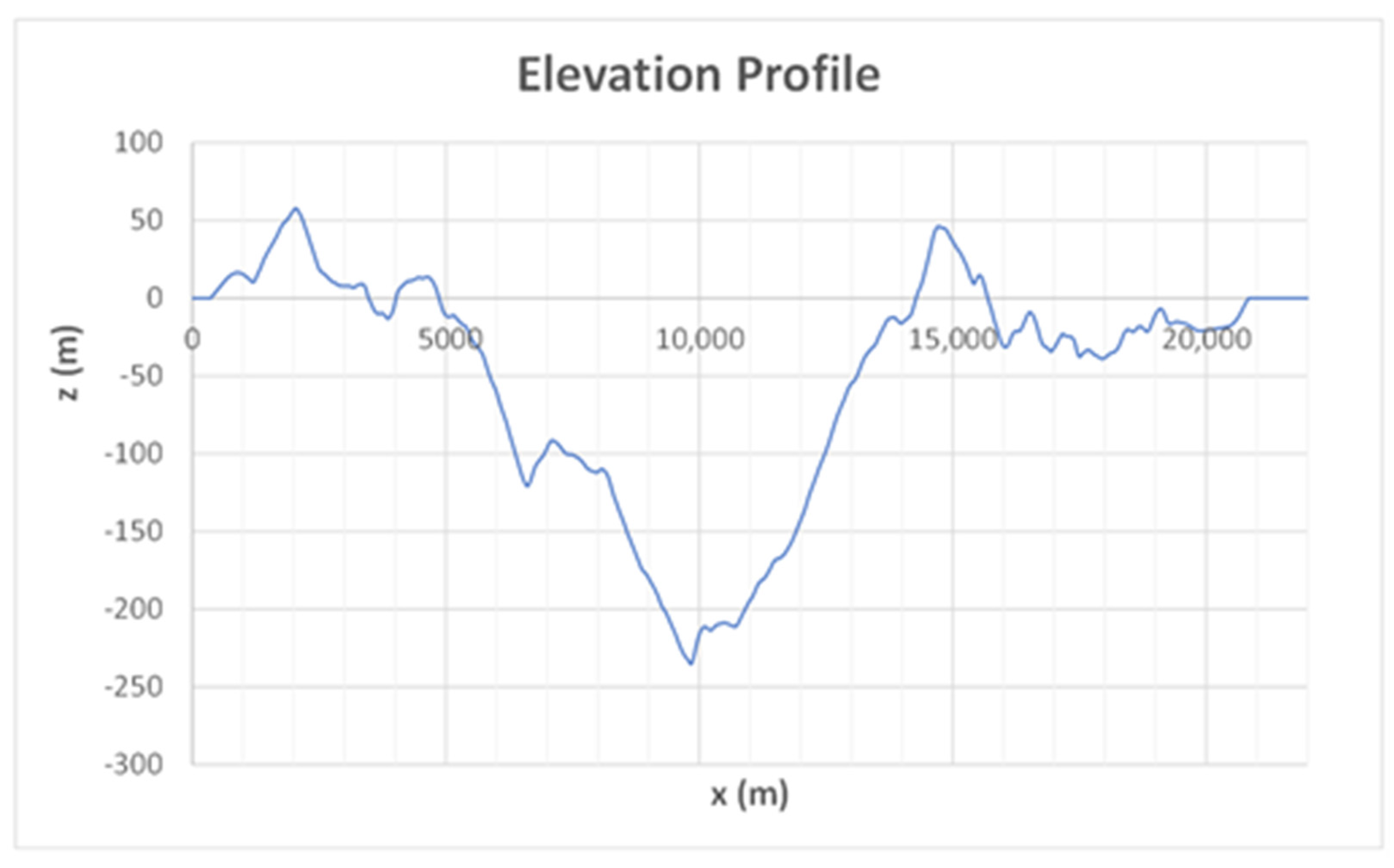
The mission of the hypercar object of this model validation is of the MotorSport type. The target speed profile for validation was obtained thanks to a maximum performance test in VI-CarRealTime on the Nordschleife variant of Nürburgring racetrack as shown in Figure 15 while Table 6 shows the main data of the target speed profile obtained and Figure 16 shows the elevation profile of the track.
4.2.6. Model Calibration
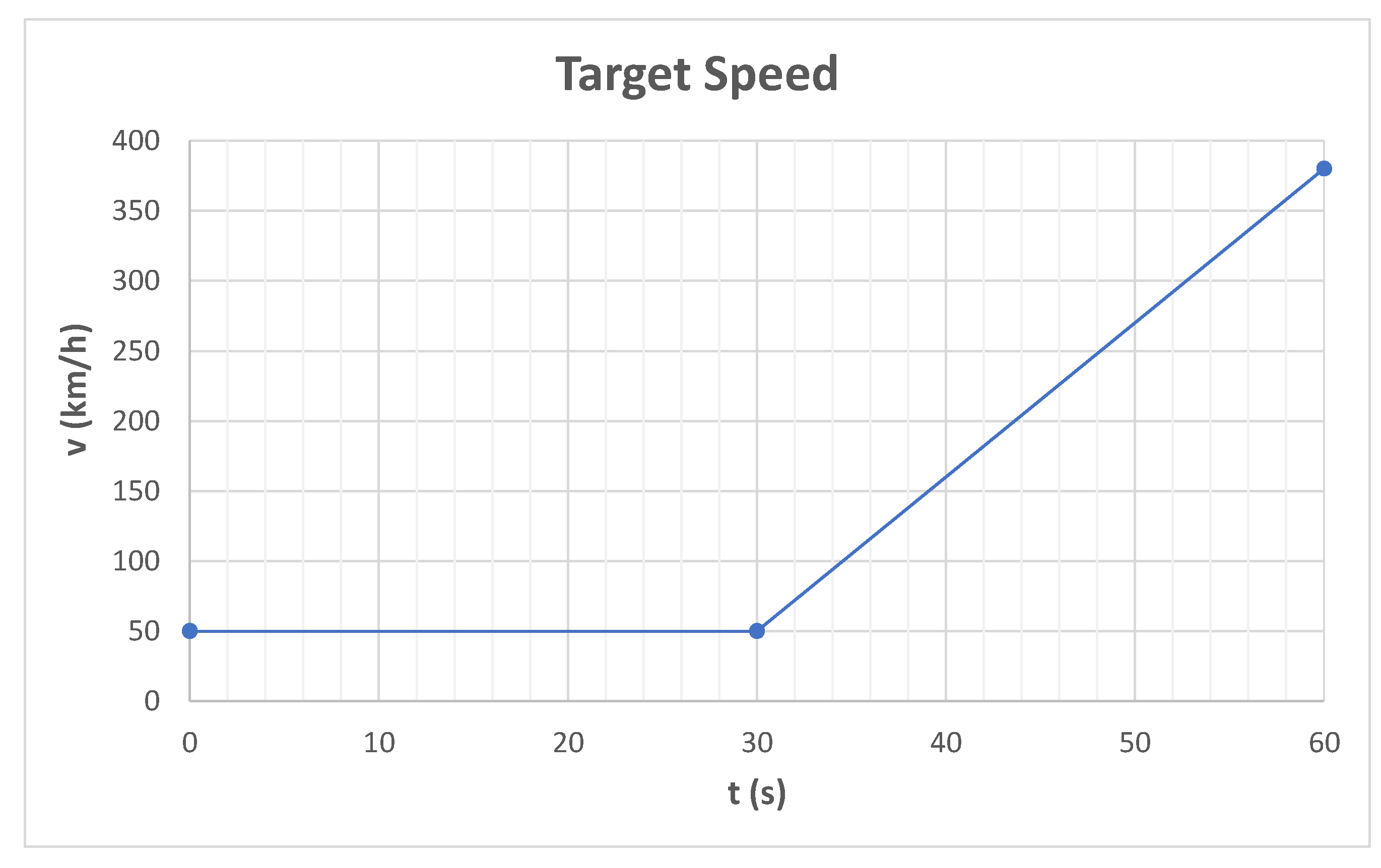
Once the results of TEST and PROPS [8] were compared, a deviation was noted between the torques required (required by the electric motors) to perform the same speed profile imposed. By isolating blocks of the program gradually, it was found that the problem arises with the balance of forces, in the TEST program the resisting forces are overestimated at low speeds, for the vehicle in question, due to the various approximations of the model. The latter therefore requires calibration. The calibration was carried out by studying the acceleration phase, imposing a speed ramp, with constant acceleration, from 50 to 380 km/h in 30 seconds. The ramp starts from 50 km/h and not from zero speed for a correct comparison with the results of the PROPS [8] program, which presents problems at low speeds (speeds close to zero).
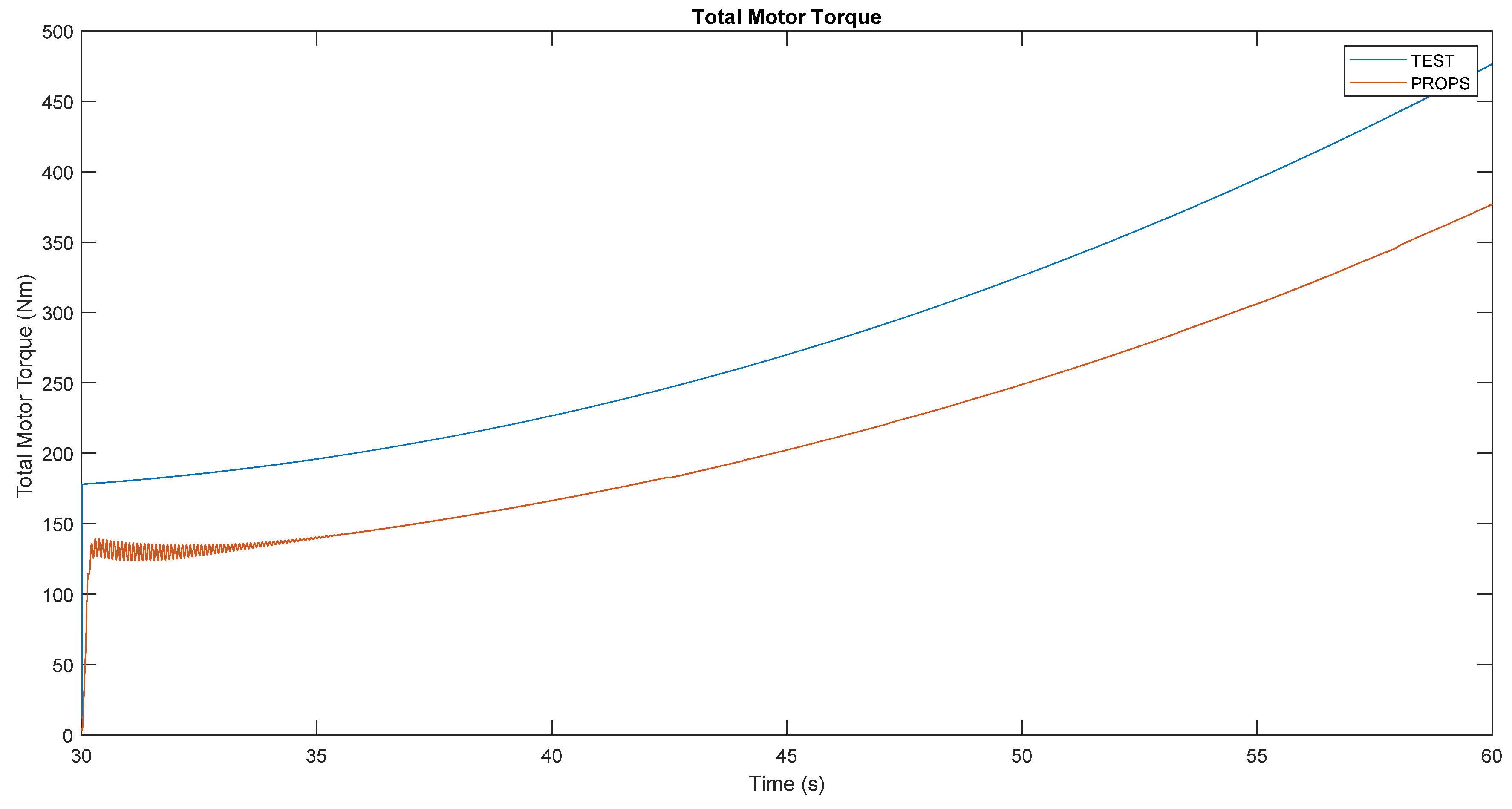
Furthermore, to allow the PROPS [8] results to stabilize, a 30-second interval at a constant speed of 50 km/h is taken before the ramp. The speed profile imposed for the simulations of TEST and PROPS [8], necessary for the calibration of the model, is shown in Table 7 and in Figure 17. For the comparison of the results between TEST and PROPS [8], the total motor torque was considered, equal to the sum of the torque delivered by the electric motor acting on the front axle with that delivered by the rear electric motor. The torques necessary for the execution of the ramp, obtained from the TEST (without calibration) and PROPS [8] programs, are shown in Figure 18.
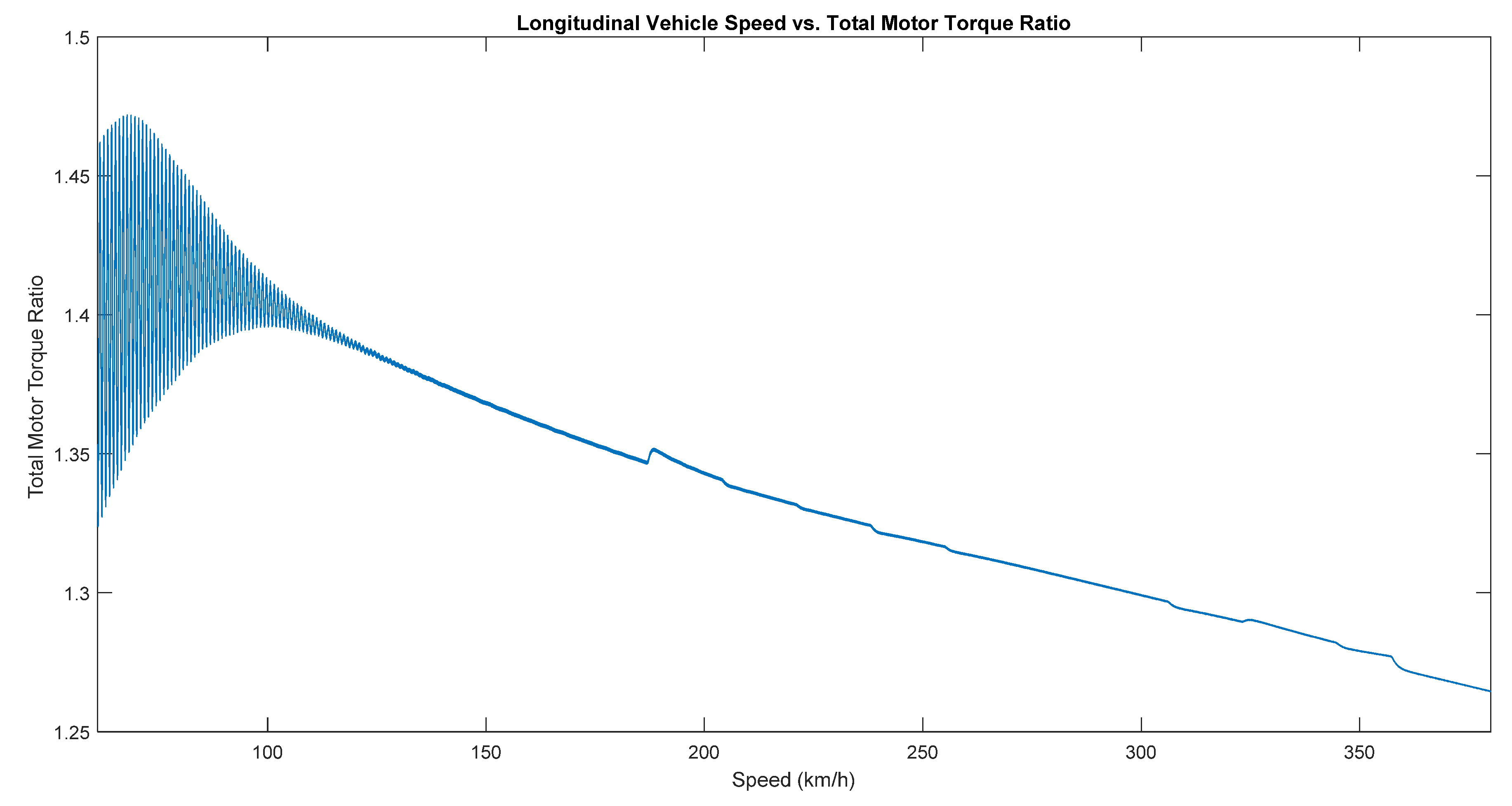
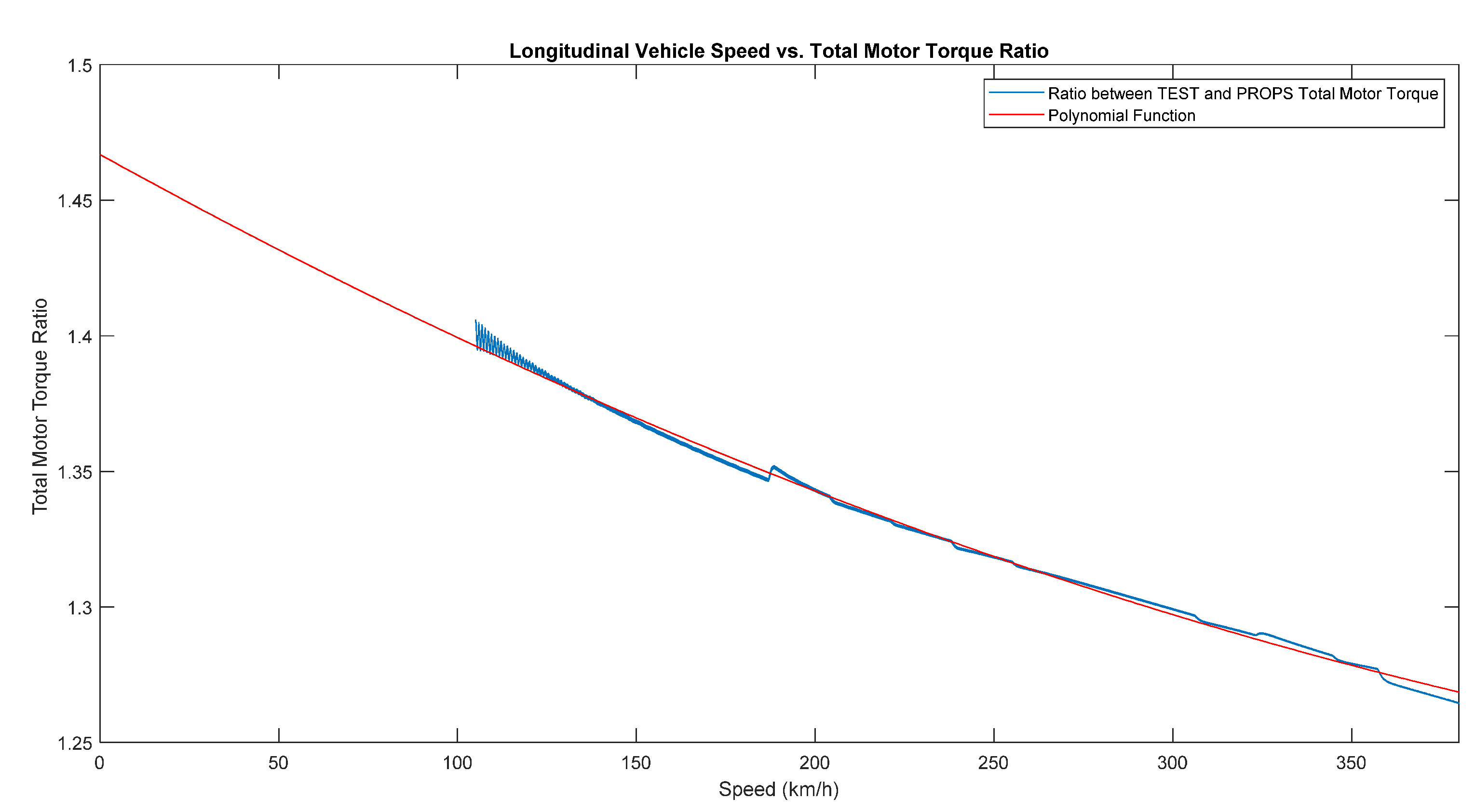
From Figure 18 it is possible to see the difference between the two torque trends. In particular, the behaviour of the ratio between the TEST and PROPS [8] torque result was analysed, represented in the Figure 19 as a function of the vehicle speed. To obtain “clean” results, the results were analysed starting from the 35 seconds elapsed from the start of the simulation. In this way the results of the PROPS [8] model have time to stabilize. The coefficients of the second-order polynomial equation that approximate the ratio between the torques were found. The result of the approximation function is shown in red in Figure 20. The function identified for the approximation is expressed unction identified for the approximation is expressed by Equation (51).
The lower order coefficient of the squared speed indicates that the ratio between the torques has an approximately linear trend as a function of the speed, in particular the results of TEST and PROPS [8] tend to realign for high vehicle speeds. Equation (51) mentioned above was then used to perform the TEST calibration for the hypercar described in Section 4.2.
4.2.7. Conditions for Validation of the Model
For the validation of the TEST model equipped with calibration, a comparison was made once again with the PROPS [8] results, this time on the speed profile of the Nürburgring obtained with VI-CarRealTime. The version of the PROPS [8] adopted does not allow to cut power to the generators if the limitations of the batteries require it, they provide constant power throughout the simulation.
Therefore, in order to also validate the electrical part of the model, it was decided to turn off both generators for the entire TEST and PROPS [8] simulations, to obtain comparable SOC, current, voltage and power data of the battery pack.
Furthermore, the same braking logic of the TEST model has also been adopted for the PROPS [8].
4.2.8. Comparison between TEST and PROPS Results
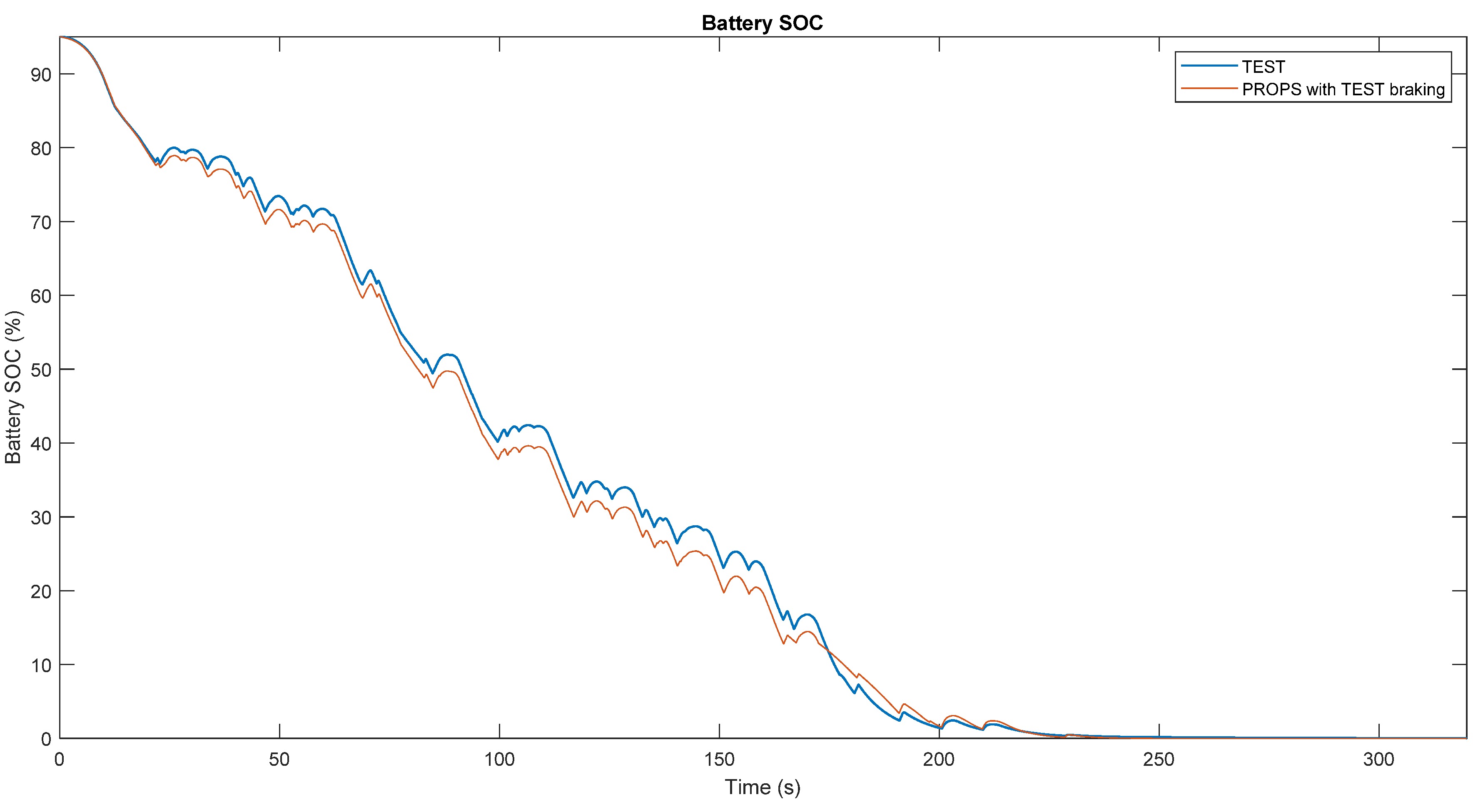
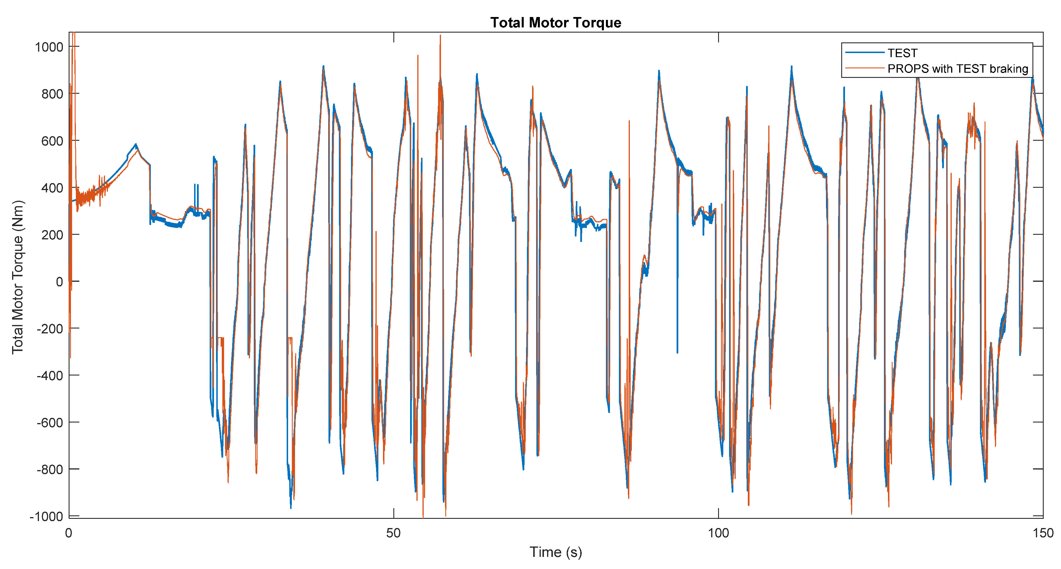
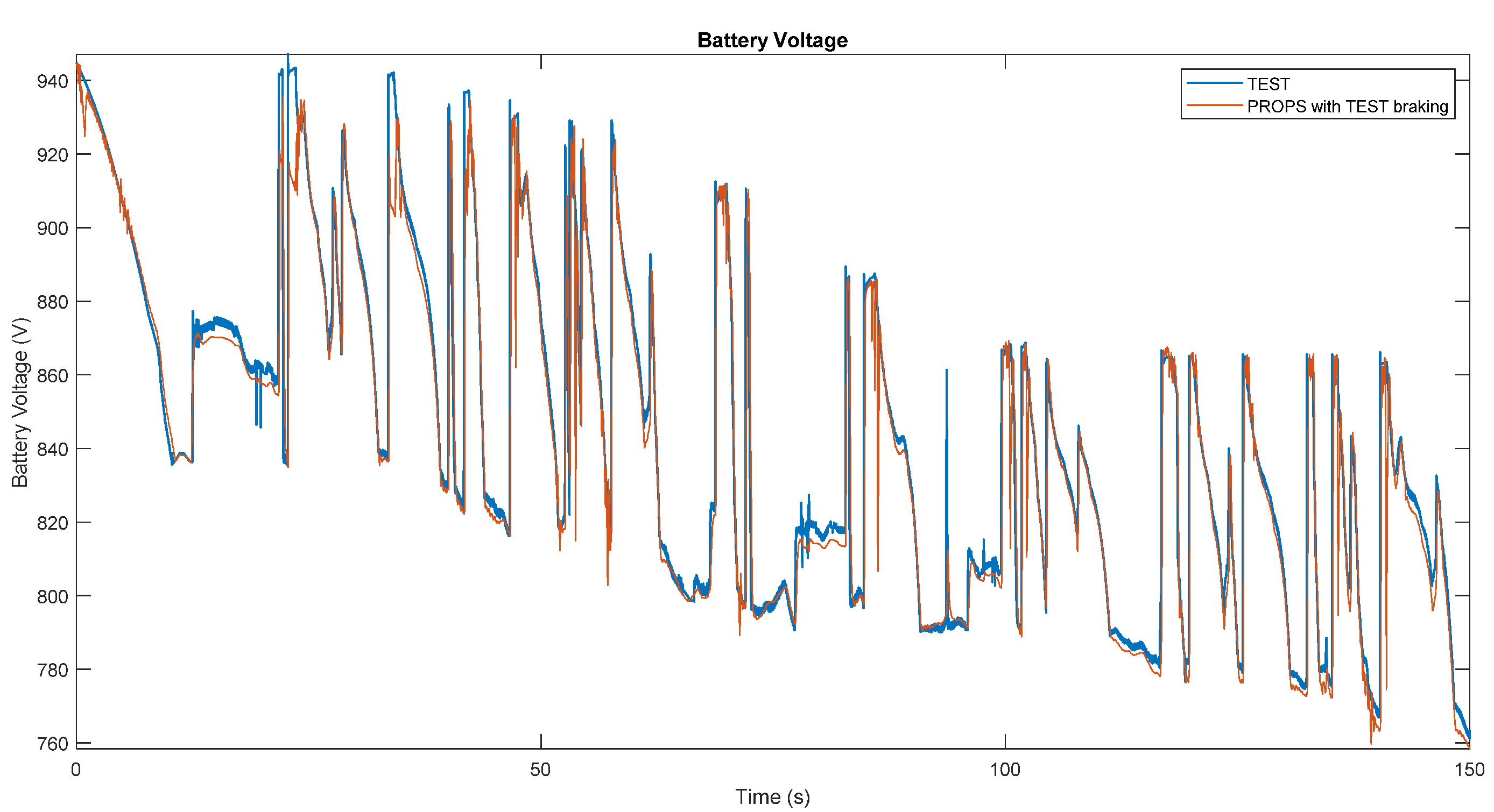
Towards the end of the simulation the battery pack is completely discharged, as can be seen from the Figure 21. To make a comparison, it is therefore better to focus on the first 150 seconds that have passed since the start of the simulation. In fact, in these first 150 seconds the battery pack has a SOC higher than about 20% and therefore there are no problems of excessively discharged pack. The results of state of charge as a function of time in TEST and PROPS [8] model are not perfectly aligned, but the difference between the two can still be considered acceptable. In the first 150 seconds the total torque results of TEST and PROPS [8] are comparable, as can be seen in Figure 22.
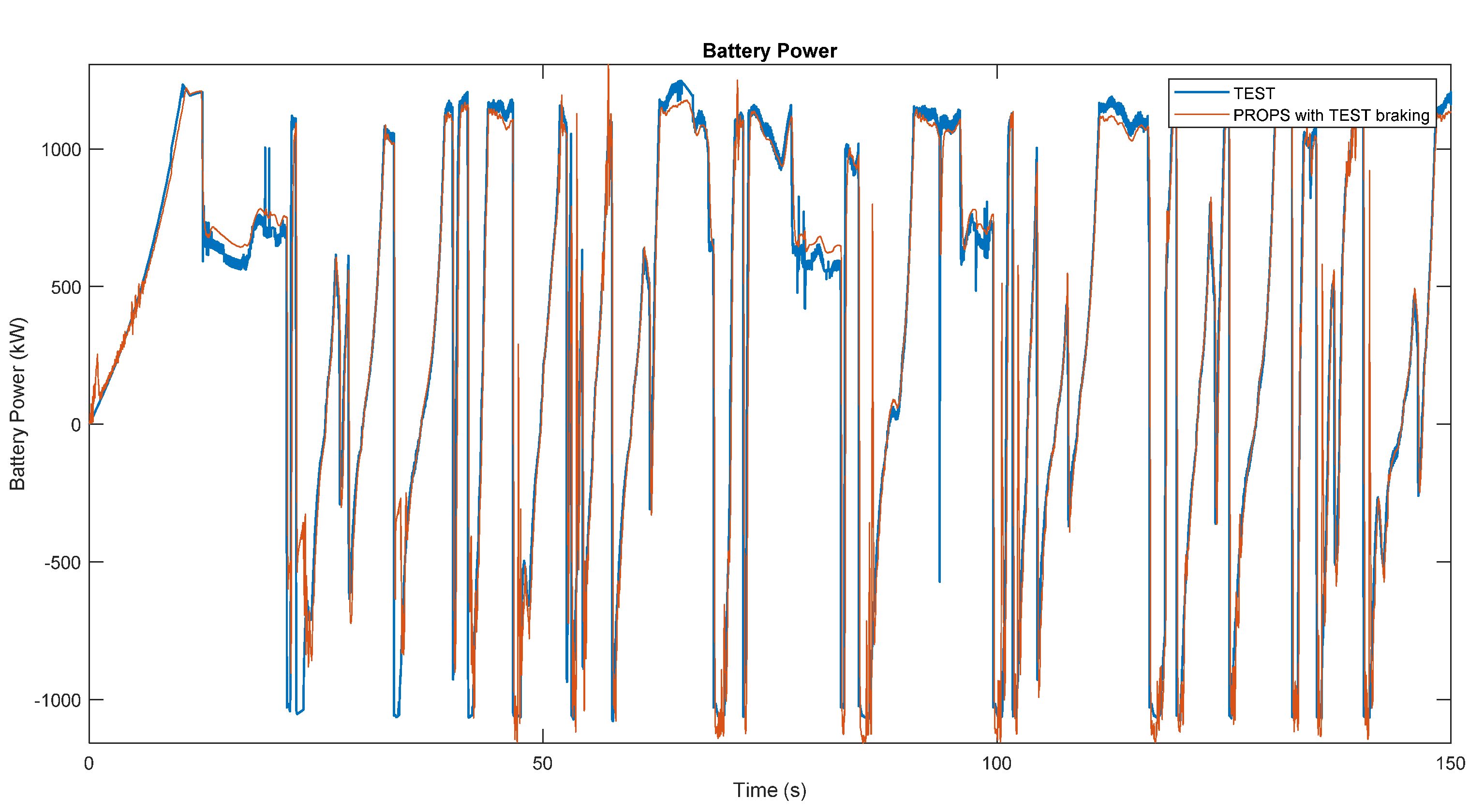
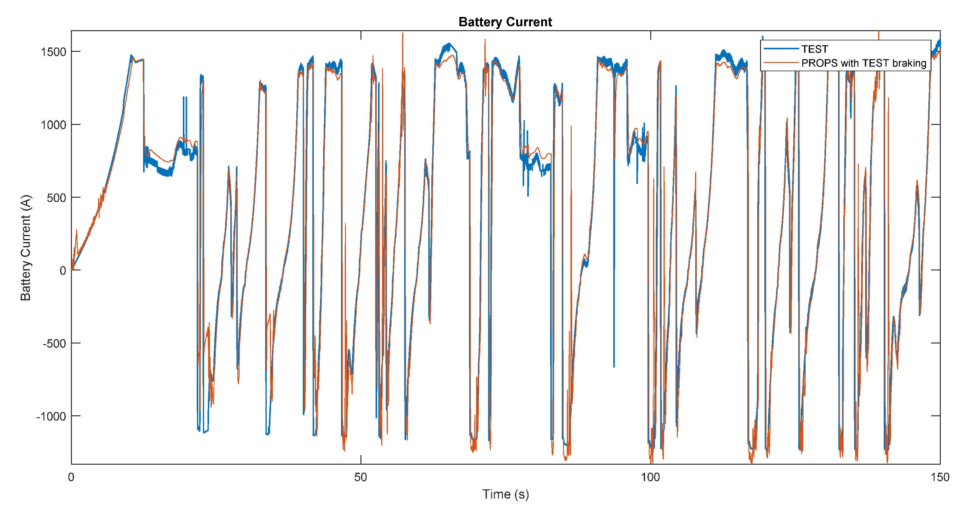
Returning to the parameters of the battery pack, also the results of power, input (negative) or output (positive) current from the pack and voltage at the battery terminals can be considered consistent between the two analysed models (always focusing on the first 150 seconds from the start of the simulation). It is possible to compare the results by observing the graphs shown in Figure 23, Figure 24 and Figure 25.
As can be seen from the graphs of Figure 22, Figure 23, Figure 24 and Figure 25, the results of the PROPS [8] program are more fluctuating. This is due to the presence of the PI controller, which is absent in the TEST model.
To obtain the performance indices of the TEST model (shown in Table 8), the error was obtained (calculated as the difference between the output parameter of the TEST model and the output parameter of the PROPS model, which has been validated with real-world data [8]) and its mean and standard deviation were calculated. The mean and the standard deviation (std) were also calculated for the absolute value (abs) of the error.
It is worth highlighting that both tools have on average the same accuracy and estimation capabilities as shown in Table 8; however, the proposed method requires a lower computational burden as it is designed using the “Backwards-Facing” technique as mentioned in Section 1, which has been proved to be more efficient. This makes this simulation tool suitable for real time applications such as driving simulators [20,21,22,23]. The same applies if compared with [13,15].
Furthermore, it is key to note that sampling time plays an important role on simulation performance, so that a sensitivity analysis has been carried out to assess its influence. In fact, when is too big the computation is faster but the final accuracy is poor due to aliasing effect, especially when is lower or close to the sampling rate of the input target speed profile. On the other hand, when is too small the computational burden grows exponentially without being justified by a substantial increase in accuracy. In general, using a sampling time between 0.05 s and 0.01 s is recommended.
5. Conclusions
The main target of this tool was to obtain shorter calculation times and perform closed-loop simulation in a more efficient way comparing to other tools reported in literature. Such tool is reliable, robust and numerically stable. It is also intuitive and easy to use for people with no specific training, thanks to a specifically designed graphical user interface. Moreover, it features the possibility to avoid any PID (or PI) controllers to perform closed-loop simulation with a target speed profile, hence avoiding complex calibration procedures. This is possible due to the “Backwards-Facing” design technique adopted for its development. The TEST simulation tool allows also to simulate performance of a multitude of hybrid or full electric powertrains with low computational burden, short simulation time and good accuracy of results. Due to the approximations adopted in the calculation of the forces, the model may require a calibration as function of the vehicle speed. The electrical part of the model requires the knowledge of all the electrical efficiencies, for calculating the power at the battery terminals. If some of these efficiencies are unknown it is possible to consider them as calibration coefficients.
Furthermore, the program is made up of several blocks, thus resulting in a program that is modular, flexible and open to simple modifications. By making the appropriate modifications to the blocks, replacing some blocks or integrating the program with additional modules, it is possible to use the model for the simulation of other types of vehicles, for example, fuel cell vehicles. This allows for high flexibility in the simulations.
Validation is also provided, based on a comparison with another consolidated simulation tool [8]. Maximum error on mechanical quantities is proved to be within 5% while it is always lower than 10% on electrical quantities.
Author Contributions
G.S. contribution was concerned to conceptualization, methodology, software, data curation and writing—original draft preparation; M.G. contribution was concerned to writing—review and editing, visualization and supervision; D.C. contribution was concerned to validation, formal analysis, writing—review and editing, data curation and supervision. All authors have read and agreed to the published version of the manuscript.
Funding
This research received no external funding.
Institutional Review Board Statement
Not applicable.
Informed Consent Statement
Not applicable.
Data Availability Statement
The data presented in this study are available on request from the corresponding author. The data are not publicly available due to University of Brescia privacy policy.
Conflicts of Interest
The authors declare no conflict of interest.
Appendix A

Table A1.
Nomenclature.
| Abbreviation | Description |
|---|---|
| Frontal area of the vehicle | |
| APU | Auxiliary Power Unit |
| Vehicle acceleration | |
| Total action areas of the brake pistons of the front callipers | |
| Total action areas of the brake pistons of the rear callipers | |
| Reference vehicle acceleration | |
| BEVs | Battery Electric Vehicles |
| Pressure portion, compared to that of the master cylinder, which acts on the front brakes | |
| BMS | Battery Management System |
| CO2 | Carbon dioxide |
| Longitudinal aerodynamic coefficient | |
| DC | Direct Current |
| The difference in distance travelled, between the current instant and the previous calculation instant | |
| The difference between the altitude of the road at the point considered and the altitude of the point of the instant of calculation preceding that considered | |
| Aerodynamic resistance, drag (calculated using vehicle speed of the previous instant of calculation) | |
| Force given by the traditional brakes | |
| Maximum force that can be generated by the braking system | |
| Force required to traditional brakes | |
| Aerodynamic resistance, drag | |
| Force lost due to inertia of the front wheels (“backward-facing” approach) | |
| Force lost due to inertia of the rear wheels (“backward-facing” approach) | |
| Static rolling resistance coefficient | |
| Rolling resistance | |
| Total traction force required at the wheels | |
| Traction force | |
| Portion of traction force which must be guaranteed by the front motor | |
| Portion of traction force which must be guaranteed by the rear motor | |
| Force lost due to inertia of the front wheels (“forward-facing” approach) | |
| Force lost due to inertia of the rear wheels (“forward-facing” approach) | |
| Additional force given by the presence of the slope of the ground | |
| Gravitational acceleration | |
| Battery pack current | |
| Charging limitation expressed as current | |
| Discharging limitation expressed as current | |
| Battery current of the previous calculation instant | |
| Theoretically required battery current (if there are no limitations) | |
| Front wheel inertia | |
| Rear wheel inertia | |
| Inertia coefficients of the moving mechanical parts in input to the reducer/gearbox of the front motor | |
| Inertia coefficients of the moving mechanical parts in input to the reducer/gearbox of the rear motor | |
| Inertia coefficient of the front electric motor | |
| Inertia coefficient of the rear electric motor | |
| Inertia coefficients of the moving mechanical parts in output to the reducer/gearbox of the front motor | |
| Inertia coefficients of the moving mechanical parts in output to the reducer/gearbox of the rear motor | |
| Local k-point mean values for the moving mean of speed profile | |
| Total length of the connection cables of the front motor | |
| Total length of the connection cables of the rear motor | |
| Binary control variable equal to 1 if there are limitations of the motors during traction due to the maximum performance of the batteries | |
| Binary control variable equal to 1 if there are limitations of the motors under braking due to the maximum performance of the batteries | |
| Binary control variable equal to 1 if there is a limitation of traditional braking | |
| Binary control variable equal to 1 if there are limitations of the generators due to the maximum performance of the batteries | |
| Binary control variable equal to 1 if there are limitations due to motors in acceleration | |
| Binary control variable equal to 1 if there are limitations due to motors under braking | |
| Driver’s mass (plus the mass of any passengers) | |
| Mass of the fuel | |
| Unladen mass of the vehicle | |
| NOx | Oxides of nitrogen |
| Number of generators | |
| Number of cells arranged in parallel inside the battery pack | |
| Number of cells arranged in series inside the battery pack | |
| Maximum power that the battery pack can absorb (by the motors and generators) | |
| Total power consumed by the vehicle accessories | |
| Available power which can be taken from the battery pack to power the motors | |
| Available power which can be taken from the battery pack to power the front motor | |
| Available power which can be taken from the battery pack to power the rear motor | |
| Total power of all cells, dissipated by Joule effect in the entire battery pack | |
| Maximum pressure that can be generated inside the master cylinder of the brake system | |
| Constant power that is used to keep within the discharge and charge limits with a defined tolerance | |
| Charging limitation expressed as power | |
| Discharging limitation expressed as power | |
| Power supplied to the batteries by the generators | |
| Nominal power of a generator | |
| Total maximum power that the generators can supply as input to the battery pack | |
| PI | Proportional–Integral controller |
| PID | Proportional–Integral–Derivative controller |
| Total power that the motors absorb from the battery | |
| Power required to the battery pack by the front motor | |
| Power required to the battery pack by the rear motor | |
| PROPS | Powertrain ROad Performance Simulation |
| Total power required to the battery pack by the motors | |
| Resistance of the single cell of the battery pack | |
| Electric resistance of the front connection cables | |
| Electric resistance of the rear connection cables | |
| Average radii of application of the braking force on the front discs | |
| Average radii of application of the braking force on the rear discs | |
| Rolling radius of the front wheels | |
| Rolling radius of the rear wheels | |
| SOC | State of Charge |
| TEST | Target-speed EV Simulation Tool |
| Front drive torque | |
| Rear drive torque | |
| Distribution of torque between the front and rear electric motors (towards the front) in the case of the accelerator pedal pressed | |
| Distribution of torque between the front and rear electric motors (towards the front) in the case of the brake pedal pressed | |
| Front motor torques required | |
| Rear motor torques required | |
| Front motor request torque (considering the motor limitation) | |
| Rear motor request torque (considering the motor limitation) | |
| Sampling time of the simulation | |
| Voltage of the battery pack | |
| Vehicle speed | |
| Vehicle speed of the instant of calculation preceding that considered | |
| Reference vehicle speed | |
| Space travelled by the vehicle | |
| Space covered by the vehicle from the start of the simulation until the calculation step preceding the one considered | |
| Power missing for the power supply of the accessories | |
| Diameter of the front motor cables | |
| Diameter of the rear motor cables | |
| Dynamic coefficients of friction between front brake pads and brake callipers | |
| Dynamic coefficients of friction between rear brake pads and brake callipers | |
| Electrical efficiencies of the front motor | |
| Electrical efficiencies of the rear motor | |
| Reference electrical efficiencies of the front motor | |
| Reference electrical efficiencies of the rear motor | |
| General efficiencies of the entire front transmission | |
| General efficiencies of the entire rear transmission | |
| Air density | |
| Electric resistivity of copper | |
| Road slope angle | |
| Reduction ratios of the front differential | |
| Reduction ratios of the rear differential | |
| Reduction ratios of the front gearbox | |
| Reduction ratios of the rear gearbox | |
| Rotation speed of the generator/s | |
| Rotation speed of the front motor | |
| Rotation speed of the rear motor | |
| Rotation speed of the front motor relative to the previous instant of calculation | |
| Rotation speed of the rear motor relative to the previous instant of calculation | |
| Reference rotation speed of the front motor | |
| Reference rotation speed of the rear motor | |
| Rotation speed of the front motor request (considering the motor limitation) | |
| Rotation speed of the rear motor request (considering the motor limitation) | |
| Reference angular speed of the front wheels | |
| Reference angular speed of the rear wheels |
References
- Automotive World, “An ICE-y Road to an Electric Future”. Available online: https://www.automotiveworld.com/articles/an-ice-y-road-to-an-electric-future/ (accessed on 9 December 2020).
- European Council, Council of the European Union, “Stricter CO2 Emission Standards for Cars and Vans Signed Off by the Council”. Available online: https://www.consilium.europa.eu/en/press/press-releases/2019/04/15/stricter-co2-emission-standards-for-cars-and-vans-signed-off-by-the-council/ (accessed on 9 December 2020).
- European Law. Brussels, 3 April 2019. PE-CONS 6/19. Regulation of the European Parliament and of the council setting CO2 emission performance standards for new passenger cars and for new light commercial vehicles, and repealing Regulations (EC) No 443/2009 and (EU) No 510/2011 (recast). Available online: https://data.consilium.europa.eu/doc/document/PE-6-2019-INIT/en/pdf (accessed on 18 February 2021).
- Ehsani, M.; Gao, Y.; Longo, S.; Ebrahimi, K. Modern Electric, Hybrid Electric, and Fuel Cell Vehicles, 3rd ed.; CRC Press, Taylor & Francis Group: Boca Raton, FL, USA, 2018; pp. 1–11. [Google Scholar]
- Bonera, E.; Gadola, M.; Chindamo, D.; Morbioli, S.; Magri, P. Integrated Design Tools for Model-Based Development of Innovative Vehicle Chassis and Powertrain Systems. In International Conference on Design, Simulation, Manufacturing: The Innovation Exchange; Springer: Cham, Switzerland, 2020; pp. 118–128. [Google Scholar] [CrossRef]
- Wu, T.; Lin, S.; Ji, X. Research on ecological environment quality management technology model based on the sustainable development of ecological theory. Fresenius Environ. Bull. 2021, 29, 10575–10580. [Google Scholar]
- Liu, A.; Zhu, J.; Yue, D.; Liu, G. Design of multi-scale expression model of ecological environment data based on wavelet transform. Fresenius Environ. Bull. 2021, 29, 9775–9781. [Google Scholar]
- Chindamo, D.; Gadola, M.; Romano, M. Simulation tool for optimization and performance prediction of a generic hybrid electric series powertrain. Int. J. Automot. Technol. 2014, 15, 135–144. [Google Scholar] [CrossRef]
- Chindamo, D.; Economou, J.T.; Gadola, M.; Knowles, K. A neurofuzzy-controlled power management strategy for a series hybrid electric vehicle. Proc. Inst. Mech. Eng. Part D J. Automob. Eng. 2014, 228, 1034–1050. [Google Scholar] [CrossRef]
- Chindamo, D.; Gadola, M. What is the Most Representative Standard Driving Cycle to Estimate Diesel Emissions of a Light Commercial Vehicle? IFAC-Pap. OnLine 2018, 51, 73–78. [Google Scholar] [CrossRef]
- Trigui, R.; Badin, F.; Jeanneret, B.; Harel, F.; Coquery, G.; Lallemand, R.; Ousten, J.P.; Castagne, M.; Debest, M.; Gittard, E.; et al. Hybrid light duty vehicles evaluation program. Int. J. Automot. Technol. 2003, 4, 65–75. [Google Scholar]
- Wang, L.; Zhang, Y.; Yin, C.; Zhang, H.; Wang, C. Hardware-in-the-loop simulation for the design and verification of the control system of a series–parallel hybrid electric city-bus. Simul. Model. Pract. Theory 2012, 25, 148–162. [Google Scholar] [CrossRef]
- Zeng, X.; Zeng, X.; Qingnian, W.; Weihua, W.; Liang, C. Analysis and Simulation of Conventional Transit Bus Energy Loss and Hybrid Transit Bus Energy Saving; SAE Paper No. 2005-01-1173; SAE International: Warrendale, PA, USA, 2005. [Google Scholar] [CrossRef]
- Tremblay, O.; Dessaint, L.-A.; Dekkiche, A.-I. A generic battery model for the dynamic simulation of hybrid electric vehicles. In Proceedings of the Vehicle Power and Propulsion Conference VPPC 2007, Arlington, TX, USA, 9–12 September 2007; pp. 284–289. [Google Scholar]
- Johnson, V.H. Battery performance models in ADVISOR. J. Power Sources 2002, 110, 321–329. [Google Scholar] [CrossRef]
- Sarathkumar, T.V.; Poornanand, M.; Goswami, A.K. Modelling and Simulation of Electric Vehicle Drive Through SAEJ227&EUDC Cycles. In Proceedings of the 2020 IEEE Students’ Conference on Engineering and Systems, SCES, Prayagraj, India, 10–12 July 2020; p. 9236717. [Google Scholar]
- Dubey, M.; Bhardwaj, S.; Harish, R.; Shyam Kumar, M.B. Simulation of Electric Vehicle using Scilab for Formula Student Application. In Proceedings of the IOP Conference Series: Earth and Environmental Science, 1st International Conference on Sustainable Energy Solutions for a Better Tomorrow, SESB, VIT, Chennai, Tamil Nadu, India, 23–24 July 2020; Volume 573, p. 012026. [Google Scholar]
- Wipke, K.B.; Matthew, R.C.; Steven, D.B. ADVISOR 2.1: A user-friendly advanced powertrain simulation using a combined backward/forward approach. IEEE Trans. Veh. Technol. 1999, 48, 1751–1761. [Google Scholar] [CrossRef]
- Guiggiani, M. Dinamica del Veicolo; Città Studi Edizioni: Turin, Italy, 1998. [Google Scholar]
- Bonera, E.; Gadola, M.; Chindamo, D.; Morbioli, S.; Magri, P. On the influence of suspension geometry on steering feedback. Appl. Sci. (Switz.) 2020, 10, 4297. [Google Scholar] [CrossRef]
- Gadola, M.; Chindamo, D. Experiential learning in engineering education: The role of student design competitions and a case study. Int. J. Mech. Eng. Educ. 2019, 47, 3–22. [Google Scholar] [CrossRef]
- Crema, C.; Depari, A.; Flammini, A.; Vezzoli, A.; Benini, C.; Chindamo, D.; Gadola, M.; Romano, M. Smartphone-based system for the monitoring of vital parameters and stress conditions of amatorial racecar drivers. 2015 IEEE Sens. Proc. 2015, 7370521. [Google Scholar] [CrossRef]
- Zhou, W.; Chen, Y.; Zhai, H.; Zhang, W. Predictive energy management for a plug-in hybrid electric vehicle using driving profile segmentation and energy-based analytical SoC planning. Energy 2021, 220, 119700. [Google Scholar] [CrossRef]
Figure 1.
Conceptual scheme of the Simulink model developed for the simulation of the longitudinal dynamics of an electric or hybrid vehicle that follows a target speed profile.
Figure 1.
Conceptual scheme of the Simulink model developed for the simulation of the longitudinal dynamics of an electric or hybrid vehicle that follows a target speed profile.

Figure 2.
The “Datasheet Battery” block and its connections with model parameters. The “Datasheet Battery” block is present in the “Simulink Library Browser” in the “Powertrain Blockset”.
Figure 2.
The “Datasheet Battery” block and its connections with model parameters. The “Datasheet Battery” block is present in the “Simulink Library Browser” in the “Powertrain Blockset”.

Figure 3.
Simulink logical scheme adopted to obtain the instantaneous vehicle speed.

Figure 4.
Different panels of the Graphic User Interface. In particular, the panels allow you to enter the inputs regarding: (a) The simulation parameters; (b) Environmental and other parameters; (c) Vehicle and Wheels parameters; (d) Brakes parameters; (e) Battery Pack parameters; (f) Motor and Transmission parameters; (g) Generators parameters.

Figure 5.
Peak torque and the continuous torque of the traction motor vs. the speed of rotation of the electric motor itself (in RPM).
Figure 5.
Peak torque and the continuous torque of the traction motor vs. the speed of rotation of the electric motor itself (in RPM).

Figure 6.
Discharge and charge current limits (in Ampere) vs. the State of Charge (SOC) of the battery pack.
Figure 6.
Discharge and charge current limits (in Ampere) vs. the State of Charge (SOC) of the battery pack.

Figure 7.
General overview of the results screen, where the abscissa axes show the time expressed in seconds. The units of measure and the parameters of the ordinate axes are shown in the legends. In the two graphs showing the acceleration and deceleration limitations, the value of the limitation is equal to one if this has intervened, 0 vice versa.

Figure 8.
Motor torque (in Nm) vs. lap time expressed in seconds. In particular, in the figure, there are the motor torque resulting from the model (in red) and the motor torque acquired through the Vehicle Control Unit (VCU) of the waste collection vehicle prototype (in blue).
Figure 8.
Motor torque (in Nm) vs. lap time expressed in seconds. In particular, in the figure, there are the motor torque resulting from the model (in red) and the motor torque acquired through the Vehicle Control Unit (VCU) of the waste collection vehicle prototype (in blue).

Figure 9.
Battery power (in kW) vs. lap time expressed in seconds. In particular, in the figure, there are the battery power resulting from the calibrated model (in red) and the battery power acquired through the VCU of the waste collection vehicle prototype (in blue).
Figure 9.
Battery power (in kW) vs. lap time expressed in seconds. In particular, in the figure, there are the battery power resulting from the calibrated model (in red) and the battery power acquired through the VCU of the waste collection vehicle prototype (in blue).

Figure 10.
Battery current (in Ampere, first graph) and the battery voltage (in Volt, second graph) vs. lap time expressed in seconds. In particular, in the figure, there are the battery current and voltage resulting from the calibrated model (in red) and the battery current and voltage acquired through the VCU of the waste collection vehicle prototype (in blue).

Figure 11.
Battery SOC vs. lap time expressed in seconds. In particular, in the figure, there are the battery SOC (in percentage) resulting from the calibrated model (in red) and the battery SOC (in percentage) acquired through the VCU (in particular from the BMS) of the waste collection vehicle prototype (in blue).

Figure 12.
Maximum motor torque vs. motor RPM. The graph is relating to the hypercar electric motors in maximum admission condition.
Figure 12.
Maximum motor torque vs. motor RPM. The graph is relating to the hypercar electric motors in maximum admission condition.

Figure 13.
Discharge (positive) and charge (negative) current limits (in Watt) vs. the SOC of the battery pack.
Figure 13.
Discharge (positive) and charge (negative) current limits (in Watt) vs. the SOC of the battery pack.

Figure 14.
OCV (Open Circuit Voltage) vs. the SOC of the battery pack.

Figure 15.
Nürburgring track, in its Nordschleife variant.

Figure 16.
Elevation profile of the Nordschleife circuit. In particular, the graph shows the elevation vs. the “longitudinal” position of the hypercar on the track (the space travelled by the hypercar on the Nordschleife circuit).
Figure 16.
Elevation profile of the Nordschleife circuit. In particular, the graph shows the elevation vs. the “longitudinal” position of the hypercar on the track (the space travelled by the hypercar on the Nordschleife circuit).

Figure 17.
Speed profile imposed for the calibration of the model, for the simulation of the hypercar.
Figure 17.
Speed profile imposed for the calibration of the model, for the simulation of the hypercar.

Figure 18.
Comparison between TEST (without calibration) and PROPS total torques during the execution of the calibration speed profile.
Figure 18.
Comparison between TEST (without calibration) and PROPS total torques during the execution of the calibration speed profile.

Figure 19.
Ratio between the TEST and PROPS torques vs. vehicle speed.

Figure 20.
Second degree polynomial (in red) that approximate the ratio between the TEST and PROPS torques (in blue).
Figure 20.
Second degree polynomial (in red) that approximate the ratio between the TEST and PROPS torques (in blue).

Figure 21.
TEST (in blue) and PROPS (in red) battery SOC (in percentage) vs. Lap Time (in seconds).

Figure 22.
This graph shows TEST (in blue) and PROPS (in red) total motor torque (in Nm) vs. Lap Time (in seconds).
Figure 22.
This graph shows TEST (in blue) and PROPS (in red) total motor torque (in Nm) vs. Lap Time (in seconds).

Figure 23.
TEST (in blue) and PROPS (in red) battery power (in kW) vs. Lap Time (in seconds).

Figure 24.
TEST (in blue) and PROPS (in red) battery current (in Ampere) vs. Lap Time (in seconds).

Figure 25.
TEST (in blue) and PROPS (in red) battery voltage (in Volt) vs. Lap Time (in seconds).

Table 1.
Main data of the waste collection vehicle.
| Parameter | Unit | Value |
|---|---|---|
| Vehicle weight | kg | 3450 |
| Front area of the vehicle | m2 | 3 |
| Drag coefficient | - | 0.7 |
| Wheels loaded radius | m | 0.35 |
| Maximum motor power | kW | 160 |
| Maximum motor torque | Nm | 380 |
| Torque limit for the regenerative braking | Nm | 50 |
| Gearbox transmission ratio | - | 21.5385 |
| Battery rated capacity at nominal temperature | Ah | 120 |
| Number of battery cells in series | - | 108 |
| Number of battery cells in parallel | - | 1 |
| OCV | V | 356.1 |
| RES | Ω | 0.097 |
| Power absorbed by vehicle accessories | W | 620 |
Table 2.
Main information of the waste collection vehicle driving cycle.
| Parameter | Unit | Value |
|---|---|---|
| Lap time | s | 600 |
| Space travelled | m | 2395 |
| Maximum speed | km/h | 31.1 |
| Minimum speed | km/h | 0 |
| Medium speed | km/h | 14.4 |
| Maximum acceleration | m/s2 | 1.8 |
| Maximum deceleration | m/s2 | −2.4 |
Table 3.
Performance indices of the waste collection vehicle simulation.
| Parameter | Mean Error | std | Abs Mean Error | std (abs) |
|---|---|---|---|---|
| Motor torque | 4.44 Nm | 13.96 Nm | 11.30 Nm | 9.33 Nm |
| Battery power | 0.58 kW | 4.18 kW | 2.66 kW | 3.28 kW |
| Battery current | 1.54 A | 12.01 A | 7.58 A | 9.43 A |
| Battery voltage | 0.18 V | 1.41 V | 0.91 V | 1.10 V |
Table 4.
Internal resistance (expressed in Ohm) of each cell in function to the SOC (from 0 to 1, first row of the table) and to the temperature in Kelvin (from 243.1 K to 313.1 K, first column of the table).
Table 4.
Internal resistance (expressed in Ohm) of each cell in function to the SOC (from 0 to 1, first row of the table) and to the temperature in Kelvin (from 243.1 K to 313.1 K, first column of the table).
| 0 | 0.2 | 0.4 | 0.6 | 0.8 | 1 | |
|---|---|---|---|---|---|---|
| 243.1 | 0.00442 | 0.00466 | 0.00451 | 0.00424 | 0.00516 | 0.00657 |
| 253.1 | 0.00319 | 0.00328 | 0.00278 | 0.00276 | 0.00302 | 0.00390 |
| 263.1 | 0.00218 | 0.00205 | 0.00203 | 0.00173 | 0.00192 | 0.00226 |
| 273.1 | 0.00102 | 0.00128 | 0.00127 | 0.00123 | 0.00136 | 0.00152 |
| 283.1 | 0.00072 | 0.00091 | 0.00090 | 0.00089 | 0.00096 | 0.00112 |
| 298.1 | 0.00028 | 0.00036 | 0.00034 | 0.00038 | 0.00037 | 0.00051 |
| 313.1 | 0.00051 | 0.00067 | 0.00050 | 0.00077 | 0.00077 | 0.00139 |
Table 5.
Main data of the hypercar.
| Parameter | Unit | Value |
|---|---|---|
| Vehicle weight | kg | 900 |
| Front area of the vehicle | m2 | 1.752 |
| Drag coefficient | - | 0.518 |
| Wheels loaded radius | m | 0.3517 |
| Maximum motor power | kW | 610.5 |
| Maximum motor torque | Nm | 530 |
| Front and rear gearbox transmission ratio | - | 2 |
| Transmission ratio of the front and rear differential | - | 3.9 |
| Maximum brake pressure in the master cylinder | MPa | 30 |
| Pressure distribution to the front in the master cylinder | - | 0.6 |
| Total area of front brake pistons | mm2 | 5058 |
| Total area of rear brake pistons | mm2 | 4084 |
| Dynamic friction coefficient of the front brake calipers | - | 0.4 |
| Operating average radius of the brake calipers | m | 0.141 |
| Battery rated capacity at nominal temperature | Ah | 6.55 |
| Operating temperature of the battery | K | 333.15 |
| Number of battery cells in series | - | 226 |
| Number of battery cells in parallel | - | 4 |
| Power absorbed by vehicle accessories | W | 400 |
Table 6.
The table shows the main information of the hypercar driving cycle.
| Parameter | Unit | Value |
|---|---|---|
| Lap time | s | 319.951 |
| Space travelled | km | 21.1 |
| Maximum speed | km/h | 389.7 |
| Minimum speed | km/h | 0 |
| Medium speed | km/h | 237.2 |
| Maximum acceleration | m/s2 | 22.2 |
| Maximum deceleration | m/s2 | −41.1 |
Table 7.
Speed profile imposed for the calibration of the model, for the simulation of the hypercar.
Table 7.
Speed profile imposed for the calibration of the model, for the simulation of the hypercar.
| Time (s) | Vehicle Speed (km/h) |
|---|---|
| 0 | 50 |
| 30 | 50 |
| 60 | 380 |
Table 8.
Performance indices of the hypercar simulation with the TEST model.
| Parameter | Mean Error | std | Abs Mean Error | std (abs) |
|---|---|---|---|---|
| Total motor torque | −15.80 Nm | 187.50 Nm | 80.00 Nm | 170.31 Nm |
| Battery power | −18.35 kW | 277.44 kW | 110.15 kW | 255.30 kW |
| Battery current | −20.03 A | 314.31 A | 125.50 A | 288.87 A |
| Battery voltage | 3.22 V | 12.39 V | 5.41 V | 11.60 V |
| Battery SOC percentage | 1.88 | 0.96 | 1.89 | 0.94 |
Publisher’s Note: MDPI stays neutral with regard to jurisdictional claims in published maps and institutional affiliations. |
© 2021 by the authors. Licensee MDPI, Basel, Switzerland. This article is an open access article distributed under the terms and conditions of the Creative Commons Attribution (CC BY) license (http://creativecommons.org/licenses/by/4.0/).
Share and Cite
MDPI and ACS Style
Sandrini, G.; Gadola, M.; Chindamo, D. Longitudinal Dynamics Simulation Tool for Hybrid APU and Full Electric Vehicle. Energies 2021, 14, 1207. https://0-doi-org.brum.beds.ac.uk/10.3390/en14041207
AMA Style
Sandrini G, Gadola M, Chindamo D. Longitudinal Dynamics Simulation Tool for Hybrid APU and Full Electric Vehicle. Energies. 2021; 14(4):1207. https://0-doi-org.brum.beds.ac.uk/10.3390/en14041207
Chicago/Turabian StyleSandrini, Giulia, Marco Gadola, and Daniel Chindamo. 2021. "Longitudinal Dynamics Simulation Tool for Hybrid APU and Full Electric Vehicle" Energies 14, no. 4: 1207. https://0-doi-org.brum.beds.ac.uk/10.3390/en14041207
Note that from the first issue of 2016, this journal uses article numbers instead of page numbers. See further details here.