Proposition of Design Capacity of Borehole Heat Exchangers for Use in the Schematic-Design Stage

Abstract

This study proposes a simple ground heat exchanger design capacity that is applicable in the schematic-design stage for several configurations used for borehole heat exchangers (BHEs). Three configurations—single, compact, and irregular types—were selected, and the heat transfer rate per unit BHE was calculated considering heat interference. In a case study with a typical configuration and general range of ground thermal conductivity, the BHE heat transfer rate of the compact configuration decreased owing to heat interference as the number of BHEs increased. However, with respect to the irregular configuration, the heat transfer rate increased as the same number increased. This was attributed to the relatively large increment rate of the distance between the boreholes in the irregular configurations, making the heat recovery factor more dominant than the heat interference. The results show that the average heat transfer rate values per BHE applicable to each configuration type in the schematic-design stage were 12.1 kW for the single configuration, 5.8 kW for the compact type, and 10.3 kW for the irregular configuration. However, owing to the large range of results for each case study, the error needs to be reduced by maximally utilizing the information available at the schematic-design stage.

1. Introduction

The design capacity of a ground-coupled heat pump system (GCHP) during the early design stage of a construction project is determined through the application of a set capacity per unit of equipment. In this work, GCHP systems refer to a heat pump coupled with vertically installed borehole heat exchangers (BHEs). However, the ground-coupled heat pump system is distinct such that the capacity and efficiency of the system are largely dependent on the design of the ground heat exchanger constituting the heat source loop, which may cause problems such as increased costs following an inaccurate early design stage. In general, the detailed estimation of an equipment system’s capacity is determined upon the completion of the building design by selecting the appropriate equipment factors to counter the acquired loads [1]. However, before the design development stage, the estimation of the approximate capacity and cost via a simple method in order to factor in the size and limitations of the entire construction project is common. The American Institute of Architects (AIA) divides the construction project process into five stages as shown in Figure 1 [2].

The schematic-design process belongs to the early stage, where the preliminary system concept is analyzed by defining the goals as well as the general scope and scale of the project. The building loads and demand are estimated in a simple way to select possible building energy systems. For instance, a building load per unit area or system capacity per unit design factor can be used that would be determined by heuristic assumption. The design development stage, which is also regarded as the early design stage, details the design process: the construction details are developed, and all the building systems are determined. In the succeeding stage, the construction documents are prepared in detail, the requirements of the client are implemented through conflict resolution and supplemental services, and the goal of the construction project is achieved. As the design progresses from the initial step of schematic design, the construction cost estimates are further subdivided, and the impact on the future revised cost is significant. Thus, there is a growing need for the establishment of a clear design from the schematic-design stage.

GCHP systems are also considered in the schematic-design stage. At this stage, an approximate GCHP capacity is estimated to elucidate the overall scale of the system without considering a detailed bore field configuration, the number of BHEs, and so on. After the approximate GCHP capacity is estimated in the schematic-design stage, whenever a change in design occurs such as in the number or configuration of BHEs or other parameters, a detailed review must be conducted through simulation in the design development stage. Here, well-known detailed design methods and commercial simulation tools can be used. In this case, repetitive feedback occurs during the review process for design proposal confirmation, resulting in additional cost and time, and the construction cost estimates in the schematic-design stage may increase in the subsequent design development stage. Conversely, excessive capacity design in the schematic-design stage can lead to the complete exclusion of the GCHP system from the project owing to the limitation of the construction cost and the client’s decision based on the estimated construction cost from the schematic-design stage. In other words, the empirical design of the GCHP system greatly increases the difference between the schematic-design stage and design development stage in some cases, and problems arising from such differences may hinder the market formation and development of the GCHP system.

In the schematic-design stage, the traditional design method is based on empirical estimates currently used in engineering handbooks or technical guidelines. The capacity of the GCHP system is estimated based on the energy demand of the building or the nominal capacity of the system [3,4,5,6], or the total length of the ground heat exchanger is calculated using the heat pump capacity [7,8]. For example, in the schematic-design stage, the reported cases of GCHP unit capacity estimation include the method of assuming ground boring to a depth of 100–200 m for the borehole heat exchanger (BHE) and connecting a heat pump of approximately 5–10 kW in capacity [9], or applying a constant capacity of 7–11 kW (≈2–3 RT (Refrigeration Ton)) per borehole for implementation in the design [10,11]. Such existing design methods are mostly based on rule-of-thumb estimation and assuming several design parameters. These methods are limited such that only very experienced and competent designers may design for an adequate capacity at the schematic-design stage [12,13]. The commonly used design method based on those rough estimations can lead to the over- or under-sizing of the GCHP system due to the following reasons.

First, the ground load is imbalanced [14,15,16,17]. Among the factors considered when designing a GCHP system, the total required length of BHEs is the most important factor since this can determine whether the required ground load is covered by BHEs or not, particularly over a long-term period. BHEs reject heat during cooling operations and extract heat in heating mode by means of heat transfer between the BHE and surrounding ground. In the ground where the BHE is installed, owing to the large heat capacity, the operation hysteresis affects the ground temperature over a long period of time. The temperature change in the ground affects the amount of heat collection (extraction) through the BHE. For example, in an area where the demand for cooling is dominant, heat is continuously injected to the ground, leading to an increase in ground temperature and, eventually, an imbalance in the ground load. This phenomenon lowers the heat exchange rate and degrades the system performance [18]. In such a case, the heat injection rate per BHE decreases, necessitating the additional installation of BHEs.

Another reason is that various bore field configurations are used for GCHP [5,19,20,21,22,23,24,25,26]. Gultekin et al. [20] investigated the heat exchange rate according to geometrical design parameters such as the spacing and number of BHEs. It is reported that a rectangular arrangement produced higher total heat transfer rates since the thermal interaction effects were smaller, while a square type, regarded as a compact and dense arrangement, showed the minimum value. Li et al. [22] investigated the thermal interaction particularly for the case of building loads unbalanced between heating and cooling, showing the differences from a single BHE case. Lazzari et al. [24] studied the long-term performance of BHEs for cases of a single BHE, a single and two staggered lines, and a square filed configuration. Compared to a single BHE, the other test cases needed a load adjustment to balance the heating and cooling ground loads.

Most of the existing studies have mainly suggested ways to increase design capacities by modifying design factors using detailed simulation tools typically employed not at the schematic-design stage but at the design development stage, as shown in Figure 1. An example is the work of Fossa and Rolando [27,28], which provided a new bore field design method based on the penalty temperature, considering the interference effect of eight surrounding BHEs, namely, Tp8. They compared the total length with the new method with the approach based on ground response functions for 240 cases of BHE fields, including squares; rectangles; I-, L-, and U-shapes; and open rectangles. They reported that the average difference is only 2.7% within a range of 10%. Their methodology provides a simplified but accurate sizing method for BHEs, but it can be used for the design development stage, as BHE locations and soil properties must be specified in detail.

Some of the studies have been conducted to provide useful design capacity information for use in the schematic-design stage. Woloszyn [29] and Li Zhu et al. [30] investigated the impact of design parameters of the GCHP on the heat exchange rates, especially for borehole thermal energy storage cases where regular arrangements were typically adopted. Ferrantelli et al. [31] proposed a simple methodology to estimate the heat transfer yield (kW) per unit length of energy piles, considering the soil types, spacing, and pile depth. Their work could be useful, but they still did not consider the thermal interference effects that are variable according to different irregular BHE arrangements.

This work aimed to propose design capacities and corresponding reference data that could be useful in the schematic-design stage of GCHP, considering unbalanced building loads, the number of BHEs, and irregular bore field configurations. All the simulations were based on the modified duct storage (DST) model proposed by Park et al. [32], as the model can describe the irregular configurations tested in this work. The following section will describe the simulation methodology, and it is followed by the results and discussion.

2. Methodology

2.1. Effects of Heat Interference among Boreholes

The effect of heat interference varies depending on the configuration of the BHE. Despite the similarity between the number and spacing of BHEs, stronger heat interference is generally observed in compact bore fields. The greater the number of boreholes, the more the imbalance in the ground load and the smaller the ground thermal diffusivity.

Figure 2 shows the heat transfer pattern of a single BHE without heat interference between adjacent boreholes and different configurations of four BHEs with heat interference. Assuming that an individual BHE is connected in parallel and heat is transferred to the ground for cooling, heat transfer from the BHE occurs as shown in the vertical section A-A’. The darker gray colors represent higher ground temperatures as a result of heat transfer from the nearest BHE or from neighboring BHEs, particularly for multiple BHE cases. Here, B is the spacing among the BHEs. The BHE at the center in the I-type bore field exhibits heat interference from two adjacent boreholes to the left and right, whereas the BHEs at both ends have heat interference from one adjacent borehole. On the other hand, in the bore field of the compact diamond configuration, each BHE is affected by three adjacent boreholes. In this case, if cooling is dominant, only a small amount of heat injected into the ground is recovered during the heating period, leading to heat accumulation in the ground and possibly stronger heat interference between the BHEs.

In this study, to analyze the heat interference effect according to the configuration type, the BHE configuration, the representative type commonly used, was selected as shown in

Table 1. Selected bore field configurations for tests.

Reference	Test Cases
Single BHE	(1) Compact	(2) 2L-shape (double lines)	(3) Rec-shape
(Single borehole)
	(4) U-shape	(5) 1L-shape (single line)	(6) I-shape

with reference to the research by Park et al. [30]. The selected configurations were a single BHE, compact BHE, and irregular BHE on a uniform grid (2L-, Rec-, U-, 1L-, and I-shapes). In Table 1, the configurations are numbered in order of strong to weak heat interference, apart from the case of a single BHE.

If the thermal properties of the ground are uniform, the heat interference effect in a specific configuration can be evaluated by the sum of the distances between BHEs as expressed in Equation (1) [30]: S is the total distance, N is the total number of BHEs, and $x_i$ and $y_i$ are the coordinates of the individual BHE as Cartesian coordinates. As an example, Figure 3 shows how to calculate S using Cartesian coordinates, and the case is the cylindrical configuration proposed in the original DST model. S can be calculated by inputting the coordinate values of the BHEs into Equation (1).

In this study, S was compared for the quantification of the heat interference effect and used for the analysis of the heat transfer rate according to the configuration.

$$S= \frac{{{\displaystyle \sum }}_{i=1}^N\left({{\displaystyle \sum }}_{j=i}^N\sqrt{{\left(x_i-x_j\right)}^2+{\left(y_i-y_j\right)}^2}\right)}{N}$$

(1)

2.2. Calculation of Heat Transfer Rates for the Bore Fields

In the case of unbalanced cooling or heating loads, the GCHP system is subject to a continuous increase or decrease in the ground temperature due to unbalanced heat extraction or injection for each year, which leads to a decrease in the coefficient of performance (COP) of the heat pump each year. Therefore, when designing a GCHP system, it must be reviewed over a long period of time to ensure that the maximum or minimum value of the entering water temperature (EWT) does not exceed the allowable design range. In general, when cooling is dominant, the maximum allowable temperature for the EWT is set within the range of 30–35 °C, and when heating is dominant, the minimum allowable temperature for the EWT is set within the range of 0–5 °C for the design of the BHE. This temperature ranges above the freezing point, but the fluid is typically an antifreeze that is a 30% propylene glycol/water mixture.

The heat transfer rate continuously decreases due to heat interference between BHEs, and to investigate this trend, two types of profiles of building loads dominated by cooling and heating were used in this study. Figure 4 represents the load pattern used in this study: (a) represents the building load dominated by cooling, and (b) represents the building load dominated by heating. Here, the cooling load is indicated as (+), and the heating load, as (−). In the case of Figure 4a, the ratio of the heating demand accounts for 16.7% of the total, while that of the cooling demand accounts for 83.3%. As shown in Figure 4b, the annual heating demand ratio is 5.7% of the total, and the cooling demand ratio is 94.3%.

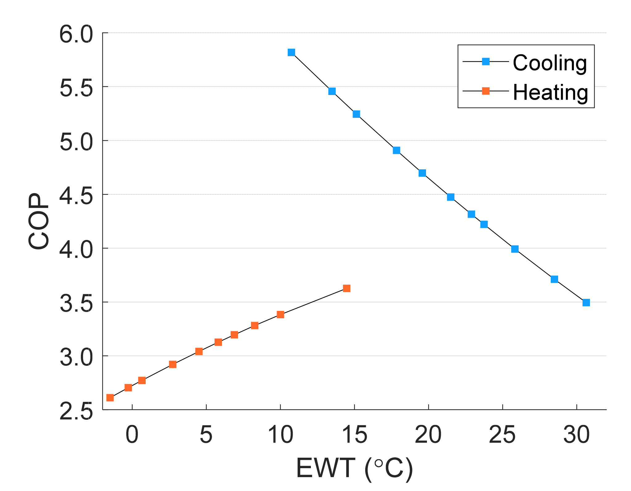
As shown in Equation (2), the building load ($Q_{\mathrm{bld}}$) can be converted to ground load ($Q_{\mathrm{g}}$) via the COP of the heat pump. The COP is an index that indicates the system performance in relation to the EWT of the GCHP. Based on the catalog data provided by the manufacturer, the COP can be expressed as a polynomial of the EWT, as shown in Equation (3). For simulation, the heat pump was modeled using Equations (2) and (3), and for all the cases, identical coefficients of α, β, and γ were applied. Based on Equation (3), the COP curve used in the test is illustrated in Figure 5, and the average heat pump COP was 4.5 for cooling and 3.7 for heating.

$$Q_{\mathrm{g}}=Q_{\mathrm{bld}}\times \left\{\begin{array}{c}1+\frac{1}{{\mathrm{COP}}_{\mathrm{c}}} \left(\mathrm{Cooling}\right)\\ 1-\frac{1}{{\mathrm{COP}}_{\mathrm{h}}} \left(\mathrm{Heating}\right)\end{array}\right.$$

(2)

$$\left\{\begin{array}{c}{\mathrm{COP}}_{\mathrm{c}} = {\alpha }_1 + {\beta }_{1}EWT + {\gamma }_1{\mathrm{EWT}}^2 \left(\mathrm{Cooling}\right)\\ {\mathrm{COP}}_{\mathrm{h}} = {\alpha }_2+ {\beta }_{2}EWT + {\gamma }_2{\mathrm{EWT}}^2 \left(\mathrm{Heating}\right)\end{array}\right.$$

(3)

The $Q_{\mathrm{g}}$ derived from the COP and $Q_{\mathrm{bld}}$ can be represented by the flow rate ($\dot{m}$) of the BHE loop, specific heat ($c_p$) of the working fluid, and heat pump $\Delta T$(=LWT − EWT), according to Equation (4). If $\dot{m}$ is constant, $\Delta T$can be determined according to the magnitude of $Q_{\mathrm{g}}$. In this study, assuming that the flow rate per BHE was constant at 0.3 kg/s, a sizing simulation of the BHE for 20 years was performed for a specific bore field case where the configuration type and number of boreholes were determined. During the 20-year simulation period, the heat transfer rate for the peak load ($Q_{\mathrm{bhe},\mathrm{peak}}$, kW) was calculated for each bore field case by adjusting the magnitude of $Q_{\mathrm{bld}}$such that the maximum EWT value of the BHEs became the desired EWT (EWT_SET) value. In the building load condition where cooling is dominant, the EWT_SET is set at 30 °C, and in the building load condition where heating is dominant, the EWT_SET is set at 0 °C.

$$Q_{\mathrm{g}}= \dot{m}\times c_p\times \Delta T$$

(4)

In order to compare the $Q_{\mathrm{bhe}, \mathrm{peak}}$ of the BHE configurations of the bore fields with numbers of BHEs between those of the single BHE configuration and other configurations, the $Q_{\mathrm{bhe}, \mathrm{peak}}$ was divided by the number of BHEs per case and expressed as the heat transfer rate per borehole (${\overline{Q}}_{\mathrm{bhe}}$). The average heat transfer rates per borehole can be compared using this rate.

2.3. Sizing Simulation for Boreholes and Calculation of Heat Transfer Rates

TRNSYS, a detailed simulation program, was used to analyze various configurations of the GCHP system. The TESS [33] library of the TRNSYS [34] program provides various types of ground heat exchanger analysis models. In this study, the duct storage (DST) model, a ground heat storage analysis model developed by Hellstöm [35], was used as the basic model. The DST model numerically calculates bore fields using a regular cylindrical configuration with a U-tube-type BHE. The DST model numerically calculates the ground heat transfer through a local and global mesh network for BHEs defined under the cylindrical coordinate system (r, z). The detailed calculation process of the DST model is presented in the work of Chapuis et al. [36]. The DST model is a well-known numerical model, and it has been validated through previous studies [23,30,37]. The volume of the heat accumulator ($V_{\mathrm{DST}}$), including the number of ground boreholes (N), spacing (B), and height (H), is defined in Equation (5). The heat transfer rate was calculated using these simple parameters. Here, the volume occupied by a single BHE was approximately equal to the volume of a cylinder with a diameter of 0.525B and a height of H (m).

$$V_{\mathrm{DST}}=\pi \times N\times H\times {\left(0.525\times B\right)}^2$$

(5)

The DST model was designed as a ground heat storage analysis model, and the configuration of the BHE was assumed to be cylindrical in all cases. Therefore, although the arbitrary modification of the cylindrical configuration of the DST model is not possible, the results from the research of Park et al. [38] were used to analyze irregular configurations other than the cylindrical configuration. In their study, the method of implementing an irregular I-shape configuration into the DST reported by Bertagnolio et al. [39] was further developed, and a rule-of-thumb equation that can depict the rectangular, U-type, and L-type configurations by modifying $V_{\mathrm{DST}}$ was proposed, as shown in Equation (6). In their paper, the DST model that uses the equation shown in Equation (6) was compared with GLHE, a commercial program, and apart from in a specific case, a difference in root mean square error (RMSE) of 5% or less was reported. Here, s represents the number of subconfigurations that can be expressed in the form of an I-shape. In the case of the L-shape configuration, the value of S is 2.

$$V_{\mathrm{DST},\mathrm{modified}}=s\times \pi \times H\times {\left[\left\{\left(NB/s\right)+B\right\}/\pi \right]}^2$$

(6)

Table 2. Simulation cases.

Parameters		Value	Unit
Number of BHEs (N)	Single BHE	1	-
	Compact	37, 91, 169, 271	-
	Irregular (2L-, Rec-, U-, 1L-, I-shape)
Ground thermal conductivity (k)	Single BHE	1.5, 2.0, 2.5, 3.0, 3.5	W/m·K

shows the numbers of boreholes, configurations, and ground thermal conductivities for the selected cases used to derive the heat transfer rate ($Q_{\mathrm{bhe}}$) for each case. Among the configurations shown in Table 1 of the previous section, 4 cases with numbers of BHEs of 37, 91, 169, and 271 were divided for the respective configurations, compact and irregular, apart from the case of a single BHE. There were 5 cases of ground thermal conductivity for each scenario, (k, W/m·K), which included 1.5, 2.0, 2.5, and 3.0 W/m·K. The compact configuration represents the configuration of the DST model included in the TESS library of TRNSYS, a building energy analysis program, and as for the irregular configuration, the DST model was modified according to Equation (6) and was depicted indirectly.

Table 3. Parameters of GCHP system simulation.

Parameter	Value	Unit
Borehole
Header depth	1	m
Borehole radius	55	mm
Borehole spacing (B)	5	m
Borehole depth (H)	150	m
U-tube spacing	23.5	mm
U-tube inside diameter	13	mm
U-tube outside diameter	16	mm
Flow rate per borehole	0.3	kg/s
Pipe thermal conductivity	0.4	W/m·K
Ground
Heat capacity	2160.5	kJ/(m3·K)
Initial temperature	15	°C
Fluid
Density	1022	kg/m3
Specific heat	3960	J/(kg∙K)
Heat pump
Average cooling COP	4.5	-
Average heating COP	3.7	-
Cooling EWTSET	30	°C
Heating EWTSET	0	°C

shows the input values required for the simulation. The values shown in Table 3 were applied in a similar manner for all the cases, and 15 °C, similar to the annual average temperature in Korea, was used for the ground initial temperature [40,41]. The BHE depth (H) was 150 m and, in the case of Korea, the same as the minimum depth eligible for subsidies for installing renewable energy equipment.

3. Results

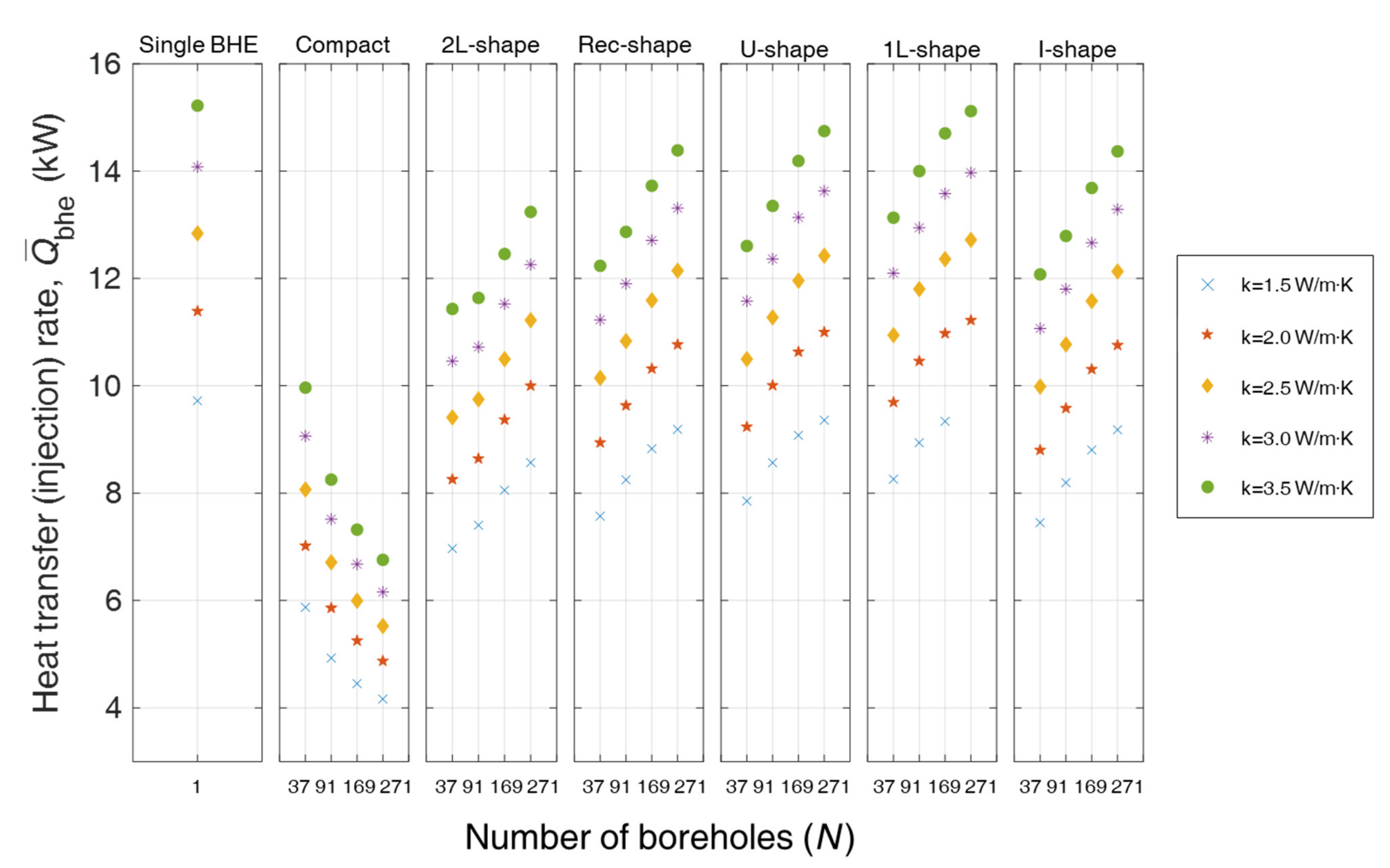
Figure 6 and Figure 7 summarize the ${\overline{Q}}_{\mathrm{bhe}}$ (kW) obtained after performing TRNSYS simulations for all the cases shown in Table 2. Figure 6 and Figure 7 each consist of seven subgraphs, and one graph corresponds to one configuration case. In Figure 6 and Figure 7, starting from the single BHE case with one BHE, the compact configuration and irregular cases (2L-, Rec-, U-, 1L-, and I-shape) are shown in the same order presented in Table 1. The x-axis of each graph represents the number of BHEs, and the y-axis represents ${\overline{Q}}_{\mathrm{bhe}}$, the heat transfer rate per borehole for each case. The upper and lower limits for ${\overline{Q}}_{\mathrm{bhe}}$ in the two figures are matched so that the differences between cooling and heating can be more readily compared. In each subgraph, when the number of BHEs is identical, the five marks indicate different ground thermal conductivities. The simulation results for the test cases are presented numerically in Appendix A,

Table A1. Results for heat transfer rate per borehole (${\overline{Q}}_{\mathrm{bhe}}$) for cooling-dominant load case.

Borehole Configurations	Number of Boreholes, N	Ground Thermal Conductivity, k (W/m·K)
		1.5	2.0	2.5	3.0	3.5
Single BHE (reference)	1	9.7	11.4	12.8	14.1	15.2
Compact	37	5.9	7.0	8.1	9.1	10.0
	91	4.9	5.9	6.7	7.5	8.3
	169	4.5	5.3	6.0	6.7	7.3
	271	4.2	4.9	5.5	6.2	6.8
2L-shape (2 line)	37	7.0	8.3	9.4	10.5	11.4
	91	7.4	8.6	9.7	10.7	11.6
	169	8.1	9.4	10.5	11.5	12.5
	271	8.6	10.0	11.2	12.3	13.2
Rec-shape	37	7.6	8.9	10.1	11.2	12.2
	91	8.2	9.6	10.8	11.9	12.9
	169	8.8	10.3	11.6	12.7	13.7
	271	9.2	10.8	12.1	13.3	14.4
U-shape	37	7.9	9.2	10.5	11.6	12.6
	91	8.6	10.0	11.3	12.4	13.4
	169	9.1	10.6	12.0	13.1	14.2
	271	9.4	11.0	12.4	13.6	14.7
1L-shape (1 line)	37	8.3	9.7	10.9	12.1	13.1
	91	8.9	10.5	11.8	12.9	14.0
	169	9.3	11.0	12.4	13.6	14.7
	271	-	11.2	12.7	14.0	15.1
I-shape	37	7.4	8.8	10.0	11.1	12.1
	91	8.2	9.6	10.8	11.8	12.8
	169	8.8	10.3	11.6	12.7	13.7
	271	9.2	10.8	12.1	13.3	14.4

and

Table A2. Results for heat transfer rate per borehole (${\overline{Q}}_{\mathrm{bhe}}$) for heating-dominant load case.

Borehole Configurations	Number of Boreholes, N	Ground Thermal Conductivity, k (W/m·K)
		1.5	2.0	2.5	3.0	3.5
Single BHE (reference)	1	8.7	10.1	11.3	12.4	13.3
Compact	37	5.1	6.0	6.8	7.5	8.1
	91	4.2	4.9	5.5	6.0	6.5
	169	3.7	4.3	4.8	5.2	5.7
	271	3.5	3.9	4.4	4.8	5.1
2L-shape (2 line)	37	6.0	7.0	7.9	8.6	9.3
	91	6.4	7.3	8.1	8.7	9.3
	169	7.0	8.0	8.8	9.5	10.0
	271	7.5	8.6	9.4	10.2	10.8
Rec-shape	37	6.6	7.6	8.5	9.3	10.0
	91	7.2	8.2	9.1	9.8	10.5
	169	7.8	8.9	9.8	10.6	11.3
	271	8.1	9.3	10.3	11.2	11.9
U-shape	37	6.9	7.9	8.8	9.6	10.3
	91	7.5	8.6	9.5	10.3	10.9
	169	8.0	9.2	10.2	11.0	11.7
	271	8.3	9.5	10.6	11.5	12.2
1L-shape (1 line)	37	7.2	8.3	9.2	10.0	10.7
	91	7.9	9.0	10.0	10.8	11.5
	169	8.2	9.5	10.6	11.4	12.2
	271	-	9.8	10.9	11.8	12.6
I-shape	37	6.5	7.5	8.4	9.1	9.8
	91	7.2	8.2	9.0	9.7	10.4
	169	7.7	8.3	9.8	10.6	11.2
	271	8.1	9.3	10.3	11.1	11.9

.

In the simulation, the ${\overline{Q}}_{\mathrm{bhe}}$ of the single BHE case without the heat interference effects between the BHEs was the highest, and as expected, the ${\overline{Q}}_{\mathrm{bhe}}$ of the compact case was the lowest, indicating the strongest heat interference. On the other hand, the configuration of the respective irregular case showed higher values than the compact case, but ${\overline{Q}}_{\mathrm{bhe}}$ was low for the configurations wherein the heat interference effects were strong, except for the I-shape case. These results were the same for all the heating and cooling load patterns.

In all the cases shown in Figure 6 and Figure 7, ${\overline{Q}}_{\mathrm{bhe}}$ increased as k increased given the same number of BHEs. This is thought to be because as the thermal diffusivity increases, ground heat transfer becomes active, thus relieving the buildup of heat or cold. In addition, as the number of BHEs (N) increased under the same k condition, the ${\overline{Q}}_{\mathrm{bhe}}$of the compact case decreased, as shown in the study of M. Kayiany [42], and the ${\overline{Q}}_{\mathrm{bhe}}$ of the irregular cases increased, showing a different trend. The reason for the difference in trend depending on the case is the difference between the increase rate of the heat interference among the boreholes and the heat diffusion rate superimposed in the surroundings. Thus, the irregular cases may make the heat recovery factor more dominant than the heat interference. This indicates that a distinction can be made between the configuration type wherein the heat interference becomes stronger and ${\overline{Q}}_{\mathrm{bhe}}$ is reduced as N increases, and another type wherein the heat interference becomes weaker and ${\overline{Q}}_{\mathrm{bhe}}$ is increased as N increases. Interestingly, despite the increase in N, the decrease in ${\overline{Q}}_{\mathrm{bhe}}$ can be prevented by a suitable setting of the bore field configuration.

Furthermore, the I-shape, which is expected to show the weakest heat interference effects among the boreholes, had a lower ${\overline{Q}}_{\mathrm{bhe}}$ overall, compared to the 1L-shape. This is thought to result from the limitation of V_DST, modified by Equation (6), which is used as the configuration analysis model. According to Park et al. [38], who proposed the model, when the I-shape was modeled using the DST model, the most irregular error was yielded, and the RMSE increased from 1.5% to 12.4% depending on the application range of the I-shape bore field. In addition, the case of the I-shape being installed at a long spacing of 5 m is unlikely to occur in actual operating conditions. The data on the I-shape case presented in Figure 6 and Figure 7 and Table A1 and Table A2 were excluded from the subsequent analysis of this study.

To verify the results for ${\overline{Q}}_{\mathrm{bhe}}$, the proposed method was compared with the commercial GLHE program [43] for selected cases as shown in Figure 6 and Figure 7. GLHE was developed for designing ground loop heat exchangers based on the finite-line-source g-function. GLHE can allow hourly calculations for estimating long-term EWTs and the total length of BHEs under user-defined bore fields. ${\overline{Q}}_{\mathrm{bhe}}$ was evaluated with GLHE for the cooling-dominant cases of a single BHE and 37 BHEs with k = 2.0, 2.5, and 3.0 W/m·K. Figure 8 shows the ${\overline{Q}}_{\mathrm{bhe}}$ differences between the proposed method and GLHE program. The ${\overline{Q}}_{\mathrm{bhe}}$ from GLHE is slightly smaller than the proposed ${\overline{Q}}_{\mathrm{bhe}}$; the average difference is 0.42 kW, which is 4.3%. This result is similar to that with the Tp8 method [28], so our proposed method can be used for a detailed sizing at the design development phase where all the required inputs for sizing are prepared.

Figure 9 shows a box plot showing the range of ${\overline{Q}}_{\mathrm{bhe}}$ according to the BHE configuration depending on the cooling/heating load case, and

Table 4. Median values of heat transfer rates per borehole (${\overline{Q}}_{\mathrm{bhe}}$, kW) for test BHE configurations.

Borehole Configuration	$$\mathbf{Median} \mathbf{Value} \mathbf{of} {\overline{\mathit{Q}}}_{\mathit{b}\mathit{h}\mathit{e}}, \mathbf{kW}$$
	Cooling	Heating
Single BHE	12.8	11.3
Compact configuration	6.4	5.1
Irregular configuration	11.2	9.3

outlines the median values of ${\overline{Q}}_{\mathrm{bhe}}$ shown in the box plot. The range expressed in the box plot shows the range of ${\overline{Q}}_{\mathrm{bhe}}$ for each configuration when the range of k is 1.5–3.5 W/m·K and the number of BHEs changes. The minimum/maximum values for each configuration are determined by a combination of the minimum/maximum value of the ground thermal conductivity and the minimum/maximum number of BHEs per configuration. For example, in the case of a compact configuration, the minimum value is obtained when the ground thermal conductivity is the lowest and the number of BHEs is 271.

In the single BHE case, the median value of ${\overline{Q}}_{\mathrm{bhe}}$ was 12.8 kW when the cooling load was dominant and 11.3 kW when the heating load was dominant, whereas in the compact configuration, ${\overline{Q}}_{\mathrm{bhe}}$ was 6.4 and 5.1 kW, respectively, for the cooling and heating scenarios, which corresponded to 0.5 and 0.45 times the values for the single BHE case. The values yielded by the irregular configuration groups were 11.2 and 9.3 kW, which corresponded to 0.88 times and 0.82 times the values for the single BHE case. In other words, in a compact bore field where the heat interference is strong, the heat extraction or injection performance of the borehole is 47% compared to in the single BHE case, and 85% in a bore field where the heat interference is relatively weak. In comprehensive consideration of these trends, this study proposes the estimation of the schematic-design capacity by referencing Table A1 and Table A2 upon the determination of the approximate configuration type, number of BHEs, and local ground thermal conductivity. Generally, the capacity per hole can vary greatly depending on the case.

Figure 10 illustrates the S value of Equation (1), which is the total distance between the BHEs according to the number of BHEs (N) per test case in the BHE configuration; the x-axis represents N, and the y-axis represents the S value. Because S, which is a quantified value of the heat interference effect between the BHEs, represents the total distance, as S increases, the heat interference between the configurations decreases. Therefore, when the number of BHEs is the same, S has the smallest value in the compact configuration and the largest value in the I-shape configuration. In the compact configuration, where ${\overline{Q}}_{\mathrm{bhe}}$ decreased as the number of BHEs increased, as shown above, the rate of increase in S according to the increase in the number of BHEs was small. By contrast, in the irregular configuration group (2L-, Rec-, U-, 1L-, and I-shapes), where ${\overline{Q}}_{\mathrm{bhe}}$ increased as the number of BHEs increased, the rate of increase in S according to the increase in the number of BHEs was large.

When these patterns are compared to the trend shown in Figure 6 and Figure 7, for configuration types such as the case of an irregular configuration wherein the effects of heat interference decrease as the number of boreholes increases, the S value increases rapidly, and for a high-density configuration, as in the case of a compact configuration, the S value shows a relatively gentle increase compared to in the other configurations. In other words, each BHE configuration type has its own N–S curve, and ${\overline{Q}}_{\mathrm{bhe}}$ increases as the number of BHE increases with a sharp increase in the N–S curve, and ${\overline{Q}}_{\mathrm{bhe}}$ decreases when the slope of the increase rate is small. In addition, if a configuration exhibits a specific increase in the N–S curve, the configuration is expected to maintain a constant ${\overline{Q}}_{\mathrm{bhe}}$ as the number increases; this point will be further investigated in a future study.

4. Conclusions

During the early design stage, determining a rough estimate of the equipment capacity is common practice. This study proposed a reference value and reference data that can be used during the schematic-design stage based on the calculation method typically implemented in the design development stage.

The heat transfer rate (kW) according to the BHE configuration type was analyzed for each configuration. For this purpose, the heat transfer rate per borehole was calculated through TRNSYS simulation with various numbers of boreholes, ground thermal conductivities, and load patterns for each configuration.

The results for the borehole configuration in the case study show that for a single BHE, based on the median value, the heat transfer rate was 12.8 kW for the cooling-dominant case and 11.3 kW for the heating-dominant case. These values were 0.45 times those for the single compact configuration, and 0.85 times those for the irregular configuration. In the compact configuration, as the number of BHEs increased from 37 to 271, the heat transfer rate per borehole decreased. In the irregular configuration, this rate increased. This was attributed to the effect of the degree of the heat interference between boreholes on the heat transfer rate depending on the configuration. In the compact configuration, as the number of BHEs increased, the heat interference between adjacent boreholes became stronger, while in the irregular configuration, the heat buildup from the heat interference between adjacent boreholes became weaker as the number of BHEs increased.

The findings of this study show that when the type of irregular configuration is taken into account during the schematic-design stage, regardless of an increase in the number of boreholes, a high heat transfer rate can be maintained. In addition, the proposed average values and data per case are expected to serve as guidelines for the estimation of the BHE capacity of ground-coupled heat pump systems during the schematic-design stage of the construction process.

References

- University of California Office of the President. UC Facilities Manual. 2019. Available online: https://www.ucop.edu/construction-services/facilities-manual/volume-3/index.html (accessed on 1 September 2020).
- The American Institute of Architects. The Architect’s Handbook of Professional Practice, 15th ed.; Wiley: New York, NY, USA, 2014. [Google Scholar]
- CEN En 12831: Heating Systems in Buildings—Method for Calculation of the Design Heat Load; BSI Standards: Brussels, Belgium, 2012.
- CEN En ISO 13790: Energy Performance of Buildings—Calculation of Energy Use for Space Heating and Cooling; BSI Standards: Brussels, Belgium, 2008.
- ASHRAE. ASHRAE Handbook—Fundamentals. Atlanta (GA): American Society of Heating; Refrigerating and Air-Conditioning Engineers (ASHRAE): Atlanta, GA, USA, 2009. [Google Scholar]
- CEN En 15450: Heating Systems in Buildings—Design of Heat Pump Heating Systems; BSI Standards: Brussels, Belgium, 2007.
- ASHRAE. ASHRAE Handbook—HVAC Applications, Atlanta (GA): American Society of Heating; Refrigerating and Air-Conditioning Engineers (ASHRAE): Atlanta, GA, USA, 2011. [Google Scholar]
- VDI. Vdi 4640-2: Thermal Use of the Underground. Ground Source Heat Pump Systems; VDI: Düsseldorf, Germany, 2001. [Google Scholar]
- Gehlin, S.E.; Spitler, J.D. Design of Residential Ground Source Heat Pump Systems for Heating Dominated Climates-Trade-Offs Between Ground Heat Exchanger Design and Supplementary Electric Resistance Heating. ASHRAE Trans. 2014, 120, 1–8. [Google Scholar]
- Lee, J.H.; Chung, M.K.; Kwak, K.S.; Park, J.H.; Lee, C.H.; Kim, H.S. Development of Installation Method of a Removal Heat Exchanger on the Ground for the Use of Geothermal Energy (KICT 2015-136); Korea Institute of Civil Engineering and Building Technology: Goyang-si, Korea, 2015. [Google Scholar]
- Ryu, H.K.; Yun, H.W.; Park, J.C. Development of Open-Loop Ground Heat Exchanger Capacity Design Tool for Large Geothermal Facilities (KRIMFI 2015-06); Korea Research Institute of Mechanical Facilities Industry: Goyang-si, Korea, 2015. [Google Scholar]
- Robert, F.; Gosselin, L. New methodology to design ground coupled heat pump systems based on total cost minimization. Appl. Therm. Eng. 2014, 62, 481–491. [Google Scholar] [CrossRef]
- Conti, P.; Grassi, W.; Testi, D. Sustainable Design of Ground-Source Heat Pump Systems: Optimization of Operative Life Performances; University di Pisa: Pisa, Italy, 2015. [Google Scholar]
- Kurevija, T.; Vulin, D.; Krapec, V. Effect of borehole array geometry and thermal interferences on geothermal heat pump system. Energy Convers. Manag. 2012, 60, 134–142. [Google Scholar] [CrossRef]
- Zhai, X.; Cheng, X.; Wang, R. Heating and cooling performance of a minitype ground source heat pump system. Appl. Therm. Eng. 2017, 111, 1366–1370. [Google Scholar] [CrossRef]
- Xi, J.; Li, Y.; Liu, M.; Wang, R. Study on the thermal effect of the ground heat exchanger of GSHP in the eastern China area. Energy 2017, 141, 56–65. [Google Scholar] [CrossRef]
- Li, W.X.; Li, X.; Wang, Y.; Tu, J. An integrated predictive model of the long-term performance of ground source heat pump (GSHP) systems. Energy Build. 2018, 159, 309–318. [Google Scholar] [CrossRef]
- Li, S.; Yang, W.; Zhang, X. Soil temperature distribution around a U-tube heat exchanger in a multi-function ground source heat pump system. Appl. Therm. Eng. 2009, 29, 3679–3686. [Google Scholar] [CrossRef]
- Qian, H.; Wang, Y. Modeling the interactions between the performance of ground source heat pumps and soil temperature variations. Energy Sustain. Dev. 2014, 23, 115–121. [Google Scholar] [CrossRef]
- Gultekin, A.; Aydin, M.; Sisman, A. Thermal performance analysis of multiple borehole heat exchangers. Energy Convers. Manag. 2016, 122, 544–551. [Google Scholar] [CrossRef]
- Signorelli, S.; Kohl, T.; Rybach, L. Sustainability of production from borehole heat exchanger fields. In 29th Workshop on Geothermal Reservoir Engineering; Stanford University Stanford: California, CA, USA, 2004. [Google Scholar]
- Li, C.; Mao, J.; Zhang, H.; Li, Y.; Xing, Z.; Zhu, G. Effects of load optimization and geometric arrangement on the thermal performance of borehole heat exchanger fields. Sustain. Cities Soc. 2017, 35, 25–35. [Google Scholar] [CrossRef]
- Fossa, M.; Minchio, F. The effect of borefield geometry and ground thermal load profile on hourly thermal response of geothermal heat pump systems. Energy 2013, 51, 323–329. [Google Scholar] [CrossRef]
- Lazzari, S.; Priarone, A.; Zanchini, E.; Priarone, A. Long-term performance of BHE (borehole heat exchanger) fields with negligible groundwater movement. Energy 2010, 35, 4966–4974. [Google Scholar] [CrossRef]
- Law, Y.L.E.; Dworkin, S.B. Characterization of the effects of borehole configuration and interference with long term ground temperature modelling of ground source heat pumps. Appl. Energy 2016, 179, 1032–1047. [Google Scholar] [CrossRef]
- Koohi-Fayegh, S.; Rosen, M.A. Examination of thermal interaction of multiple vertical ground heat exchangers. Appl. Energy 2012, 97, 962–969. [Google Scholar] [CrossRef]
- Fossa, M.; Rolando, D. Improved Ashrae method for BHE field design at 10 year horizon. Energy Build. 2016, 116, 114–121. [Google Scholar] [CrossRef]
- Fossa, M.; Rolando, D. Improving the Ashrae method for vertical geothermal borefield design. Energy Build. 2015, 93, 315–323. [Google Scholar] [CrossRef]
- Wołoszyn, J. Global sensitivity analysis of borehole thermal energy storage efficiency for seventeen material, design and operating parameters. Renew. Energy 2020, 157, 545–559. [Google Scholar] [CrossRef]
- Zhu, L.; Chen, S.; Yang, Y.; Tian, W.; Sun, Y.; Lyu, M. Global sensitivity analysis on borehole thermal energy storage performances under intermittent operation mode in the first charging phase. Renew. Energy 2019, 143, 183–198. [Google Scholar] [CrossRef]
- Ferrantelli, A.; Fadejev, J.; Kurnitski, J. A tabulated sizing method for the early stage design of geothermal energy piles including thermal storage. Energy Build. 2020, 223, 110178. [Google Scholar] [CrossRef]
- Park, S.-H.; Jang, Y.-S.; Kim, E.-J. Using duct storage (DST) model for irregular arrangements of borehole heat exchangers. Energy 2018, 142, 851–861. [Google Scholar] [CrossRef]
- Thornton, J.W.; Bradley, D.; McDowell, T. TESS Component Libraries for TRNSYS 16; Thermal Energy Systems Specialists LLC: Madison, WI, USA, 2005. [Google Scholar]
- Klein, S.; Beckman, A.; Mitchell, W.; Duffie, A. TRNSYS 17-A TRansient SYstems Simulation Program; Solar Energy Laboratory, University of Wisconsin: Madison, WI, USA, 2011. [Google Scholar]
- Hellström, G. Duct Ground Heat Storage Model, Manual for Computer Code; Department of Mathematical Physics, University of Lund: Lund, Sweden, 1989. [Google Scholar]
- Chapuis, S.; Bernier, M. Seasonal Storage of Solar Energy in Borehole Heat Exchangers. In Proceedings of the 11th International IBPSA Conference, Glasgow, UK, 27–30 July 2009; pp. 599–606. [Google Scholar]
- Kim, E.-J. TRNSYS g-function generator using a simple boundary condition. Energy Build. 2018, 172, 192–200. [Google Scholar] [CrossRef]
- Park, S.-H.; Kim, E.-J. Optimal Sizing of Irregularly Arranged Boreholes Using Duct-Storage Model. Sustainability 2019, 11, 4338. [Google Scholar] [CrossRef] [Green Version]
- Bertagnolio, S.; Bernier, M.; Kummert, M. Comparing vertical ground heat exchanger models. J. Build. Perform. Simul. 2012, 5, 369–383. [Google Scholar] [CrossRef]
- Kim, Y.K.; Jo, J.S.; Lee, D.H.; Sohn, B.H.; Lee, T.W. Long-term variations of ground temperature in a medium sized geothermal heating and cooling system. In Proceedings of the Society of Air-conditioning and Refrigerating Engineers of Korea Summer Annual Conference, Yongpyong, Korea, 27–29 June 2012; pp. 758–761. [Google Scholar]
- Lee, M.J.; Choi, J.K.; Hwang, K.M.; Kim, W.S.; Lee, W.J.; Choi, S.M. Standard Design Guideline of New & Renewable Energy System for General Buildings; Korea Energy Agency: Yongin-si, Korea, 2010. [Google Scholar]
- Kaviany, M. Principles of Heat Transfer in Porous Media, 2nd ed.; Springer: New York, NY, USA, 1995. [Google Scholar]
- Spitler, J.D. GLHEPRO-A design tool for commercial building ground loop heat exchangers. In Proceedings of the Fourth International Heat Pumps in Cold Climates Conference, Aylmer, QC, Canada, 17–18 August 2000. [Google Scholar]
Figure 1.
The five main stages of a construction project and the ground-coupled heat pump system (GCHP) design process in the early stage.
Figure 2.
Heat interference effects according to BHE configuration.
Figure 3.
Example of BHE coordinates for calculating the total distance according to Equation (1).
Figure 4.
Test building load: (a) cooling-dominant case and (b) heating-dominant case.
Figure 5.
Heat pump entering water temperature (EWT)–coefficient of performance (COP) curve for heating and cooling cases.
Figure 6.
Variation in the heat transfer rate () for test configurations of bore field (cooling-dominant case).
Figure 7.
Variation in the heat transfer rate () for test configurations of bore field (heating-dominant case).
Figure 8.
Comparison between proposed and GLHE (reference) .
Figure 9.
Range of heat transfer rates per borehole (, kW) according to test BHE configurations.
Figure 10.
Different S values according to increase in N for test bore field configurations.