1. Introduction
As the power sector offers the greatest cost-effective potential for emission reductions compared with other sectors, such as heat and transport, cost-optimized strategies to limit global warming to below 2 °C typically have close to zero emissions in the power sector by the middle of the century [
1]. However, energy system optimization models (ESOMs) usually only consider direct, on-site CO
2 emissions when assessing the cost-optimized design of infrastructure components of future electricity supply (e.g., power plants, storage facilities, and grids).
Life cycle assessments (LCAs) quantify the potential impacts of technologies and processes across a comprehensive set of environmental categories, covering entire life cycle chains, associated emissions, and ecologically relevant extractions from the environment [
2]. The LCA literature on renewable energy conversion technologies showed that they are associated with higher upstream energy demand compared to conventional technologies and higher corresponding indirect (i.e., not caused by the combustion of fuels on site) greenhouse gas (GHG) emissions and other environmental impacts per unit of capacity [
3]. Thus, concerns have been raised that these may affect the emissions reduction potential of low-carbon technologies and that other environmental stressors may be overlooked [
4]. ESOMs with high spatial and temporal resolution analyze cost-optimized, long-term strategies to meet the emission limitations implied by climate targets [
5]. However, indirect emissions, especially those related to the energy required for the construction of power plants and the production and transport of fuels and other inputs, are usually not considered in those models. Thus, the inclusion of data on life cycle impacts in ESOMs is a promising approach in order to overcome the shortcomings of “classical” ESOMs. Due to their complementary nature, the combination of ESOMs and LCAs is an emerging field of research and can guide energy policy to achieve energy systems with improved overall environmental performance.
To date, life cycle indicators have mostly been linked to model output in order to estimate environmental impacts (also called “ex-post assessment”). For example, Berrill et al. [
6] showed that systems largely based on variable renewable energy (VRE) perform better for most impact categories but have larger resource depletion and land occupation impacts than systems based on fossil energy options. Hertwich et al. [
7] compared the global BLUE Map and the business-as-usual scenarios from the International Energy Agency (IEA) and found that low-carbon technologies allow for the reduction of pollution-based impacts, while metal demand increases. Xu et al. [
8] confirmed the results of the latter two studies for European electricity scenarios, pointing out in particular the high land requirements of photovoltaic (PV) installations. Luderer et al. [
9] assessed scenarios from various integrated assessment models (IAMs) and showed that environmental effects largely depend on the choice of technology and that mitigation efforts tend to increase resource and land use impacts in line with the former studies.
While such approaches provide meaningful insights into the environmental performance of given scenarios, they do not take full advantage of the model’s capabilities to determine environmentally improved system configurations compared to original model setups (e.g., pure cost optimization with upper limits for direct CO
2 emissions). More specifically, solutions are overlooked that internalize (also called “model-endogenous integration”) life cycle environmental impacts. In the literature, integration efforts are manifold and range from the setting of upper limits for certain indicators to the monetarization of emissions and indicators to multi-objective optimization. For example, Daly et al. [
10] set upper limits on both direct and indirect CO
2 emissions in an ESOM for the UK and found that mitigating the total emissions nearly doubles the marginal abatement costs compared to the consideration of direct CO
2 emissions only. McDowall et al. [
11] took a similar approach with a focus on Europe and showed that limiting indirect GHG emissions increases the use of wind power, while the expansion of solar PV declines. Algunaibet et al. [
12] downscaled the eight planetary boundaries defined by Ryberg et al. [
13], which aim to provide a safe space for humanity, to the US power sector and showed that compliance with the upper limits leads to a doubling of system costs compared to the cost-optimal solution. Portugal-Pereira et al. [
14] considered a tax on both direct and indirect GHG emissions for part of the energy system studied. This led to a shift towards the use of technologies that did not consider indirect emissions and underlined the importance of integrating indirect emissions for all technologies that can be expanded in an ESOM. Another study by Pehl et al. [
15] followed a similar approach but covered GHG emissions for all technologies optimized endogenously. The authors showed that a tax on indirect GHG emissions, as opposed to a tax on direct emissions only, leads to an increased expansion of concentrated solar power (CSP), wind, and nuclear power plants. An aggregated environmental indicator was included in the optimization function by Rauner and Budzinski [
16] covering the German electricity supply. Applying multi-objective optimization, the authors showed that an environmentally sustainable system leads to increased deployment of VRE, particularly wind energy, compared to an unconstrained cost-optimal system based mainly on fossil fuels. Multi-objective optimization integrating costs and life cycle impacts was conducted by Tietze et al. [
17] and applied to an exemplary residential quarter. In several model runs that considered different impacts, the authors showed a number of different system configurations resulting from different weightings of environmental impacts and highlighted the importance of including the life cycle perspective in the design of energy systems. Vandepaer et al. [
18] optimized both the system costs and life cycle impacts and then included predefined system cost constraints in the optimization of environmental impacts for the Swiss energy system. The authors demonstrated that a small increase in costs can result in substantial climate change mitigation. However, this statement is based on only a small selection of solutions explored.
At present, however, the consideration of life cycle GHG emissions as an additional objective to system costs is still very limited. Furthermore, the ESOMs in most of the latter studies have a low temporal and/or geographical resolution and are therefore not able to fully capture the feed-in of VRE and the resulting impact on auxiliary infrastructures such as storage and grid. We overcome these limitations with the integration of life cycle impacts into the spatiotemporal high-resolution ESOM “Renewable Energy Mix” (REMix). The model is particularly designed to assess the infrastructural demand for a reliable power supply. We use a comprehensive set of life cycle inventories (LCIs) of up-to-date electricity supply, distribution, storage, and conversion technologies. The life cycle indicators generated rely on harmonized LCIs that consider the evolutions in their upstream life cycles by incorporating the effects of future decarbonization measures in the global electricity sector (such future-oriented applications of LCAs are also known as “prospective LCAs” [
19]). To evaluate the effect of the reduction of life cycle GHG emissions on system costs, we apply multi-objective optimization and calculate a pareto front. This concept was first introduced by Vilfredo Pareto and allows for the systematic assessment of trade-offs between conflicting objectives [
20]. In addition, we analyze the occurrence of burden shifts over several life cycle impacts for the solutions explored. The extended ESOM is applied to Europe and North Africa (EUNA). Specifically, our aim is to answer the following research questions:
What are the trade-offs between total system costs and life cycle GHG emissions for the future electricity system in EUNA?
How does the structure of the power system and the grid change when life cycle GHG emissions are reduced?
What are the trade-offs that occur regarding further life cycle environmental impacts?
Our research is particularly useful for energy and environmental policy makers aiming for cleaner power generation considering the entire upstream supply chain.
This article is structured as follows:
Section 2 presents the methodology and the case study,
Section 3 illustrates the results of the case study,
Section 4 presents the discussions, while
Section 5 draws the main conclusions from the work.
2. Materials and Methods
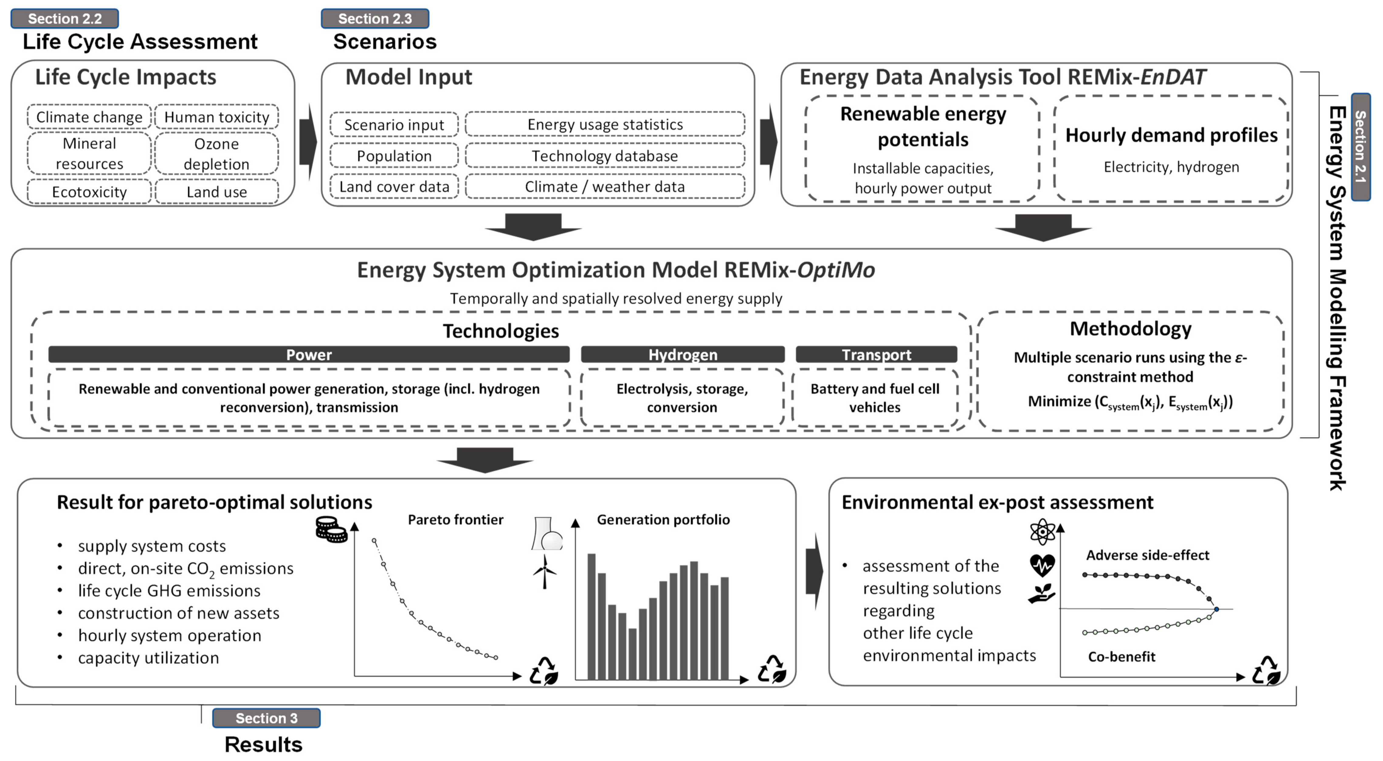
Figure 1 illustrates the workflow of this study and the corresponding sections of the paper in which we provide details on the different steps.
The approach consists of two main parts: ESOM on the one hand and life cycle impacts for the technologies considered on the other hand. The ESOM used in this study is REMix, which is extended by an algorithm that enables multi-objective optimization (see
Section 2.1). The LCI database used provides the technology specific indicators for the ESOM (see
Section 2.2). We use a specific scenario setup for this case study based on earlier work (see
Section 2.3). Then, multi-objective optimization is performed using techno-economic parameters and the life cycle indicators (in this case study, GHG emissions). In addition, environmental ex-post assessment is conducted for the resulting pareto optimal solutions. Details on the modeling approach developed are described in the next section.
2.1. Extended Energy System Model to Perform Multi-Objective Optimization
In this chapter, we first explain the general structure of the REMix modeling framework and then describe the adjustments necessary to calculate the life cycle indicators for the power system and to perform multi-objective optimization.
2.1.1. The Traditional REMix Modeling Framework
A comprehensive description of REMix and the corresponding equations are provided in Gils et al. [
21]. In short, the model consists of two main elements: the energy data analysis tool (REMix-EnDAT) and the optimization model (REMix-OptiMo) (
Figure 1). REMix-EnDAT performs the VRE resource assessment in high spatial and temporal resolution. It provides hourly generation profiles for the main technologies aggregated to user-defined regions. In addition, electricity demand profiles are generated in this part of the model. The supply and demand profiles are used in REMix-OptiMo to determine the most cost-effective operation and expansion of all system components during every hour of the year. REMix-OptiMo is a deterministic linear optimization program in a formulation of a general algebraic modeling system (GAMS). The model is built in a modular structure with a wide range of technology modules (e.g., a module for storage technologies) that are largely independent of each other. In each module, the parameters, variables, equations, and inequalities used to represent the respective technical and economic characteristics are defined. Power generation, storage and grid technologies are represented by their installed and maximum installable capacities, their investment and operating costs, and their efficiencies. All technology modules allow for the operation and expansion of the technologies considered. Additions of power plants, transmission lines or storage capacities can be optimized by the model according to the existing potentials and system requirements. Investments in new capacities consider technology costs, payback periods, and interest rates.
In short, the model:
Minimizes the total system cost, which consists of investment costs (treated as annuities) and the operating costs of the entire system;
Decides on the size of energy storage (power capacity, energy capacity), hydrogen storage, grid, and generation technologies;
Considers a one-year modeling horizon (in our case the year 2050) with full hourly resolution (i.e., 8760 time steps) for which the optimal operation of each technology at each modeling node is determined.
In previous studies, REMix was used to estimate the cost-optimal design of energy systems and has been applied in several studies, ranging from case studies for specific regions [
22,
23,
24,
25,
26,
27], model comparisons [
28] to comprehensive model coupling [
29]. The model adaptions necessary to consider LCA-based indicators in the REMix are described in the next section.
2.1.2. Extension of the REMix Modeling Framework
For the purpose of this study, two new modules are introduced to REMix-OptiMo. The first module collects all investment and dispatch variables of the different technologies and calculates the system-wide life cycle impacts, which can also be used for environmental ex-post assessments. This module also contains the description of the second objective function (Equation (1)) next to systems costs. Note that for the sake of clarity, we simplified the notation (e.g., planning year or technology sets are neglected) compared with that implemented in REMix. In the present study, the second objective function to be minimized summarizes the life cycle GHG emissions of all technologies considered to the overall life cycle GHG emissions. It is composed of the GHG emissions of all added capacities
(Equation (2)), with
being the endogenous optimization results,
the corresponding technology specific impacts (e.g., per GW
electricity), divided by the calendrical lifetime of the plant
to account for the single year time horizon of the model calculation. Operation dependent life cycle impacts
(Equation (3)) consist of the sum over each time step
of the hourly generation of added
as well as existing capacities
multiplied with the corresponding life cycle impacts related to operation
(e.g., per GWh
electricity). The term is multiplied by the efficiency ratio between the LCI data
and the ESOM
to correct for differences in assumptions on efficiencies. Existing capacities can be defined exogenously. In addition, we include a penalty for unsupplied power
.
In the second module, the augmented epsilon-constraint method (
ε-CM) described by Mavrotas [
30] is implemented to perform multi-objective optimization to assess the trade-offs between system costs and life cycle GHG emissions. The pareto front covers the solution space between the minimum cost and the least GHG emission-intensive solution. Compared to a weighted objective function, the
ε-CM offers the advantages of finding solutions that are not supported by weighting and of avoiding sensitivities to scaling. In addition, it allows for a systematic exploration of pareto-efficient solutions. A description of the approach adopted can be found in
Appendix A.
The adaptions of the LCIs necessary to populate the REMix model with life cycle indicators for the different technologies (i.e., for deriving and ) are described in the next section.
2.2. Life Cycle Assessment
The aim of this study is to quantify life cycle impacts of meeting the electricity demand of the EUNA region in 2050, considering all upstream activities in the supply chain of energy technologies. For this purpose, we base this study on the Framework for the Assessment of Environmental Impacts of Transformation Scenarios (FRITS) that uses the ecoinvent 3.3 cut-off background LCI database [
31]. The framework was developed to assess the life cycle impacts of existing energy system scenarios on different sectoral and geographical scales and contains the LCI data used in this case study.
2.2.1. Foreground Life Cycle Inventory Data and Technology Mapping
In LCA, LCI data are differentiated into fore- and background data. Foreground data are those that describe the system that is the focus of the analysis; background data are those supporting the modeling of the foreground system. In our case, foreground LCI data represent the technologies in REMix. Therefore, the technologies presented in REMix must be mapped to the appropriate LCI data sets based on the technical specifications described in both sources. The LCI data for energy technologies that are missing in the ecoinvent 3.3 database (e.g., stationary battery storage, high-voltage direct current (HVDC) electricity grid, electrolyzers) are collected from scientific sources and integrated into the LCI database. The full list of technologies and corresponding LCI data sources are listed in
Appendix B,
Table A2.
2.2.2. Adjustments of Fore- and Background Life Cycle Inventory Data
In LCAs, operations- and infrastructure-related datasets are usually aggregated into one LCI dataset. We therefore disaggregate the LCI data into operations- and infrastructure-related processes for each technology to match the corresponding decision variables in REMix.
FRITS enables the consideration of regional adjustments of the global background power generation mix. In the present study, the 2 °C scenario by Teske et al. [
32] is applied to the background database, which describes region-specific power mixes until the main feature of renewable energy technologies is that a large proportion of the environmental impact occurs in the upstream supply chain of these technologies. Changes in the electricity system affect the environmental impacts caused, in particular, by the manufacturing processes. Thus, we capture important improvements in the electricity system that provides electricity in the manufacturing of power plants, storage and conversion technologies, and electricity grids.
A challenge in coupling LCA-based environmental impacts to geographically large-scale ESOMs is to avoid double counting of environmental impacts in the background LCI database. More specifically, the LCI for processes in the upstream supply chain (e.g., steel production) may include energy flows from processes that are already within the boundary defined in the ESOM (e.g., electricity production). In this study, we avoid double counting for the electricity sector by matching the markets for electricity generation in ecoinvent with the regions in REMix (see
Tables S2 and S3). Subsequently, we delete all of the input flows (e.g., electricity production by a wind turbine) from these markets. This approach to avoid double counting in the background has already been implemented in the earlier application of FRITS [
31], and similar approaches have been used in other work as a possible option to address this challenge [
15,
33,
34].
In addition, double counting also occurs in operation depended foreground data sets (e.g., electricity as input to electrolysis). Thus, these flows are removed from the respective LCI data sets.
2.2.3. Life Cycle Indicators
In the final step, we generate life cycle indicators that provide the environmental scores of the different impact categories for the technologies and integrate them as parameters into the model (see
Section 2.1.2).
In this paper, indicators are calculated using the International Reference Life Cycle Data System (ILCD) 2.0 2018 impact assessment method that translates thousands of LCI entries (e.g., NO
X and PM
2.5) to sixteen mid-point impact categories using a variety of environmental mechanisms [
35] (
Table 1). The method was selected because it was the most up to date at the time the study was conducted and was developed in a transparent and scientifically sound process. Furthermore, the characterization factors were adapted for the ecoinvent database used.
The technology-specific indicators integrated in REMix are listed in
Table S4 of the Supplementary Materials. Life cycle CO
2eq emissions represented by the impact category “climate change” are used as an additional objective in the ESOM. The other indicators are applied in environmental ex-post assessment of the different solutions. Note that in the following, life cycle CO
2eq emissions, which also include emissions other than carbon dioxide, such as ethane, methane or nitrogen fluoride, are referred to as life cycle GHG emissions and CO
2 emissions are the direct, ESOM-based emissions (traditional scope of REMix).
The information considered in the ESOM for the adjustment of the LCA indicators is efficiency and lifetime to ensure consistency and to allow for the correct consideration of the impacts from construction (see Equations (2) and (3)), in line with earlier integration work [
16,
18].
2.3. Scenario Setup
Our scenario setup is based on the model parameterization and the “CSP&H2” scenario in combination with the “Trend” scenario for transmission grid expansion defined in Cao et al. [
36]. The “Trend” scenario assumes that all major ten-year network development plan (TYNDP) projects [
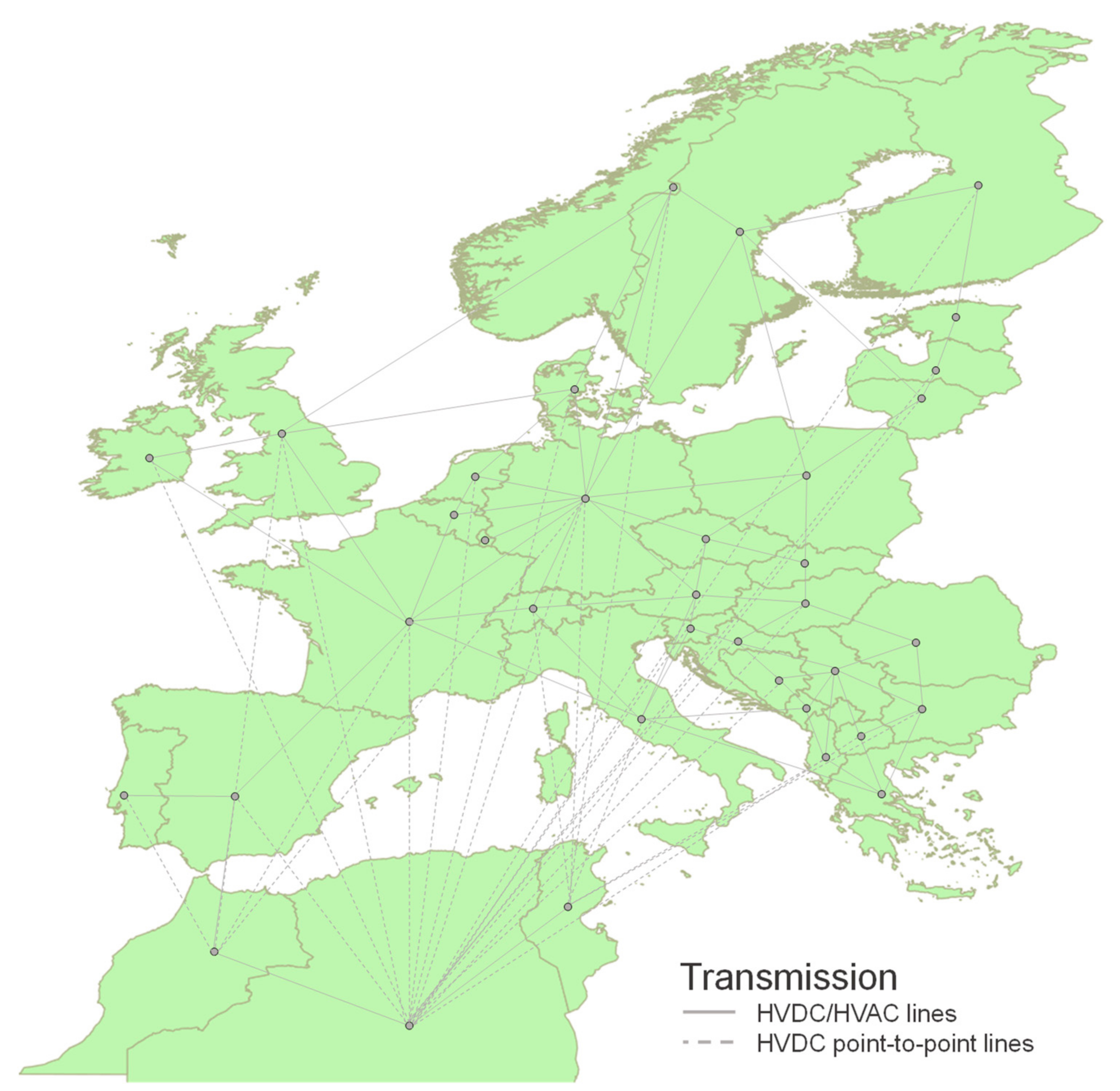
37] are implemented and the current structure of the transmission network will be maintained. New expansion in the high and extra-high voltage network is possible. Note that REMix also allows for the expansion of cables (ground embedded overland cables in combination with submarine cables), which are presented separately from lines (aerial lines in combination with submarine cables) in this work.
A certain part of power plant capacities is defined exogenously. For conventional power plants, the commissioning date from the World Electric Power Plants Data Base (WEPP) [
38] is combined with lifetime assumptions to determine the phase-out date. The capacities remaining in the scenario year are assumed model-exogenous for the modeling. Model-exogenous capacities for PV and wind power plants are derived from Reference [
37]. Wind power plants are divided into on- and offshore plants and PV into open ground and rooftop plants. The country-specific distribution is done as follows: For wind, one half of the wind power generation capacity given in the data set is divided according to the current onshore–offshore ratio, determined from Reference [
39]. The other half is divided according to the ratio of maximum installable generation capacities based on the potential analysis in REMix-EnDAT. PV is allocated exclusively according to the ratio of the maximum installable generation capacities based on the potential analysis. Hydropower plants are differentiated into run of river, pumped storage, and reservoir hydropower plants. For the installed capacities and their geographical allocation, a data set from the Frankfurt Institute for Advanced Studies (FIAS) is used [
40]. There is no model-exogenous specification of generation capacities for biomass and geothermal. Note that in the following, the life cycle environmental impacts as well as the system costs are composed of exogenously defined as well as added capacities.
For the sake of simplicity, the heat sector is not considered in the present study. This is the main difference with the scenario setup by Cao et al. [
36], who, for example, also considered the additional electricity demand by heat pumps, electric boilers, and the heat demand to be covered by cogeneration.
In short, the scenario setup has the following characteristics:
Regions: European countries (ENTSO-E members), with the exception of Turkey, Iceland, Cyprus, and Ukraine; North African countries: Algeria, Morocco, and Tunisia.
Figure 2 illustrates the spatial resolution and the representation of the power grid;
Technological and sectoral scope: Fossil, nuclear, and renewable power generators, energy storage for load balancing, electricity exchange, and hydrogen transport (via H
2 pipelines) among model nodes. Furthermore, we allow direct electricity imports via HVDC lines from North Africa to Europe as specified by Hess [
25,
26]. Concerning the sectoral scope, we consider the power system as well as additional electricity and hydrogen demand for electric and H
2 vehicles. The electricity and hydrogen demand for mobility is specified exoge-nously. Hydrogen production and storage are optimized endogenously. All assumptions on specific investment, operation, and maintenance costs are listed in
Table S1 of the Supplementary Materials;
Constraints: To allow regional flexibility in achieving CO
2 reduction targets on direct emissions of ~95% compared to 1990, we define a CO
2 cap (~60 Mt) for the entire model region. This cap is based on country-specific annual energy balances [
41] for electricity generation and fuel-specific CO
2 emission factors [
42]. Recall that the renewable potentials derived from REMix-EnDAT (including hydropower plants) constrain the maximum installable capacity of renewable technologies. In addition, nuclear power is restricted to currently installed capacities and projects planned in countries where it is permitted in line with assumptions used in the project “analysis of the European energy system under the aspects of flexibility and technological progress” (REFLEX) and follow-up publications [
43,
44,
45]. This results in maximal installable capacities of ~131 GW, most of which can be located in France (~63 GW). Furthermore, we distribute the power and hydrogen generation capacities across EUNA by setting country-specific self-supply thresholds of 80% in terms of annual demand (see Equation (A5) in
Appendix A).
The use of 80% of the self-sufficiency ratio for electricity and hydrogen generation is based on expert judgement deduced in an internal workshop from preliminary model runs.
The annual electricity demand amounts to 3062 TWh for conventional consumers, 263 TWh for electric vehicles and 570 TWh for H2 vehicles. Note that final inputs for REMix are hourly time series of electricity and hydrogen consumption. The optimization is performed using weather data from the year 2006, which was a year with average capacity factors compared to other available years in REMix-EnDAT. Since it is our goal to investigate a variety of system configurations, we calculate 20 pareto-efficient points for the scenario setup.
3. Results
We first focus on the trade-offs between system costs and life cycle GHG emissions in
Section 3. Subsequently, we analyze the structure of the power system and the power grid for the individual solutions on the pareto frontier (
Section 3.2). Co-benefits and adverse side effects with respect to further life cycle environmental impacts are analyzed in
Section 3.3 (ex-post assessment of solutions on the pareto front).
3.1. Trade-Offs between System Costs and Life Cycle Greenhouse Gas Emissions
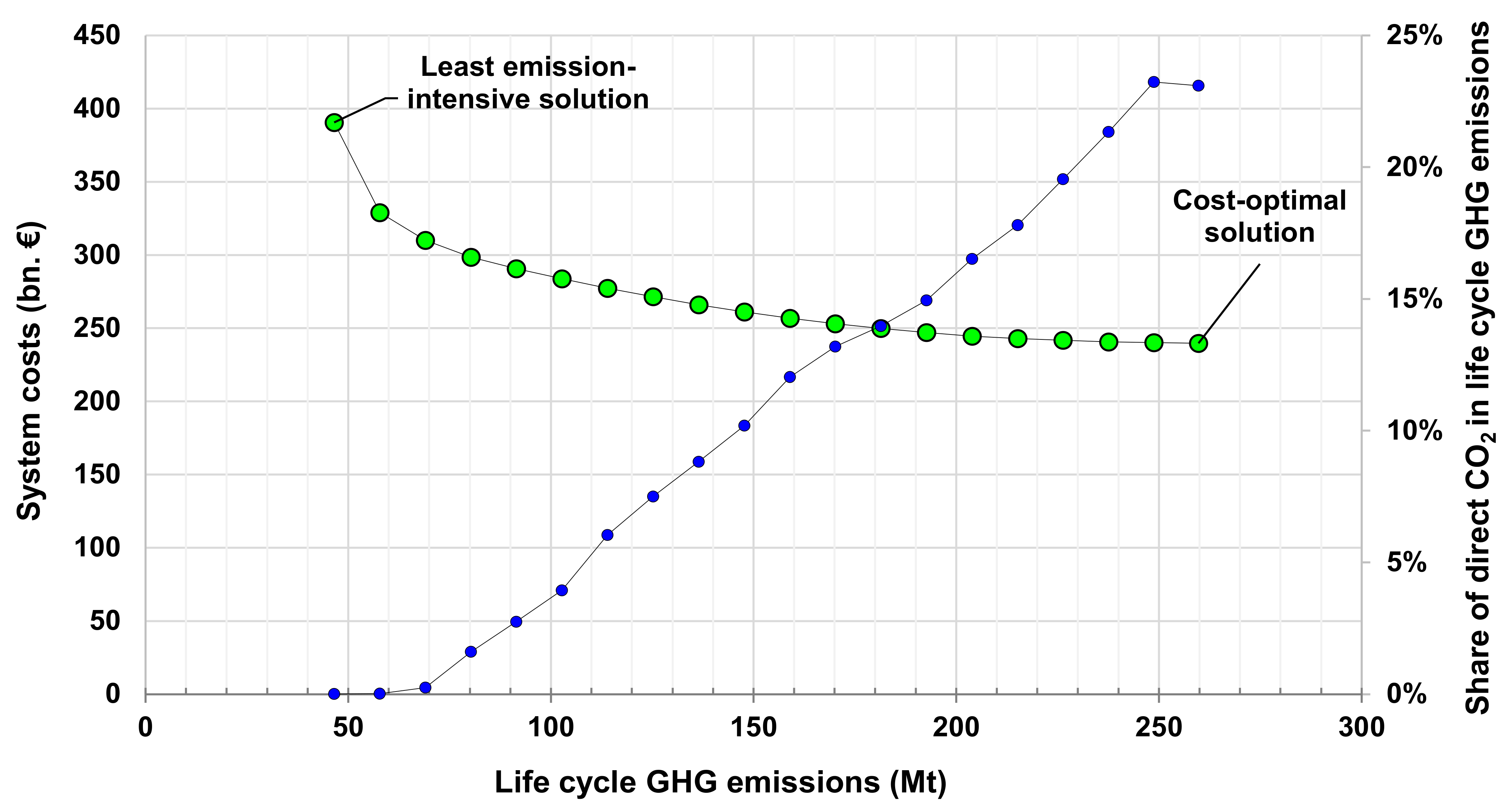
The pareto front illustrated in
Figure 3 represents the trade-offs between system costs and climate impacts for both life cycle GHG emissions (green dots) and the share of direct CO
2 emitted due to the energy system operation (blue dots). Each point on the pareto front represents an energy system in the year According to the implementation of the
ε-CM, the solution of the point in the upper left represents the point with least GHG emissions, whereas the point on the very right represents the system with the least costs. Finally, the solutions for the points between these two extrema result from minimizing system costs while constraining life cycle GHG emissions for a given threshold. Starting at the least cost-intensive solution, this threshold is increased in equidistant steps.
Following the pareto front from right to left, we initially see a strong decline in life cycle GHG emissions in relation to rising system costs. More specifically, 22% (i.e., from 260 Mt to 204 Mt) of life cycle GHG emissions could be mitigated with an increase in system costs of 2%. This range of solutions could be described as the “low-hanging fruit” of a cost efficient, comprehensive, climate-friendly electricity supply. A reduction in life cycle GHG emissions by approximately two-thirds (from 260 Mt to 91 Mt) is accompanied by an increase in system costs of 21%. A further reduction is theoretically possible to 18% of the initial emissions. The cost increase in this case is 63% compared to the cost-optimal solution.
In the cost-optimum solution, the carbon footprint of the electricity mix is 67 g CO
2eq/kWh; whereas, in the system with least GHG emissions, it decreases to 12 g CO
2eq/kWh. Compared to the current electricity mix for Europe (409 g CO
2eq/kWh) [
46], this is a reduction of 84% or 97%, respectively.
As expected, the reduction in life cycle GHG emissions also leads to a reduction in direct CO2 emissions. With a 6% cost increase compared to the cost optimum, life cycle GHG emissions reduced by 34% (to 170 Mt) and direct CO2 emissions by 63% (to 22 Mt). This drop in direct emissions continues and reaches 100% in the last two solutions. As life cycle GHG emissions are reduced, the relative cost differences between the individual solutions grow. This is particularly evident in the last two points on the pareto front (i.e., the reduction of emissions by 78% (to 58 Mt) and 82% (47 Mt) compared to the cost optimum).
From an LCA perspective, the impacts associated with electricity supply in increasingly ambitious systems are being shifted from operations to the manufacturing of the generation infrastructure: whereas direct CO2 emissions account for 23% of the total life cycle GHG emissions in the cost optimum, their share drops to 0% in the solution with least life cycle GHG emissions. At this point, all GHG emissions are caused by background processes. This highlights the need for full emissions accounting in future assessments of ambitious energy systems. It also shows that technologies with low GHG emissions upstream in the supply chain are crucial for ambitious energy systems, as their direct counterparts can almost be omitted with still moderate cost increases. Note, however, that while the LCI database has been adapted to reflect low carbon future electricity supply, other emission-intensive processes, such as fossil fuel-based heat in industry and freight transport, remain at the current state on the database. Further adjustments in these sectors would reduce upstream GHG emission and thereby increase the share of direct CO2 emissions in total life cycle GHG emissions.
To better understand the roles of individual technologies for the solutions on the pareto front, we next analyze the resulting mix of power generators and technologies for temporal and spatial load balancing in the power system.
3.2. Structure of the Power Plant Portfolio
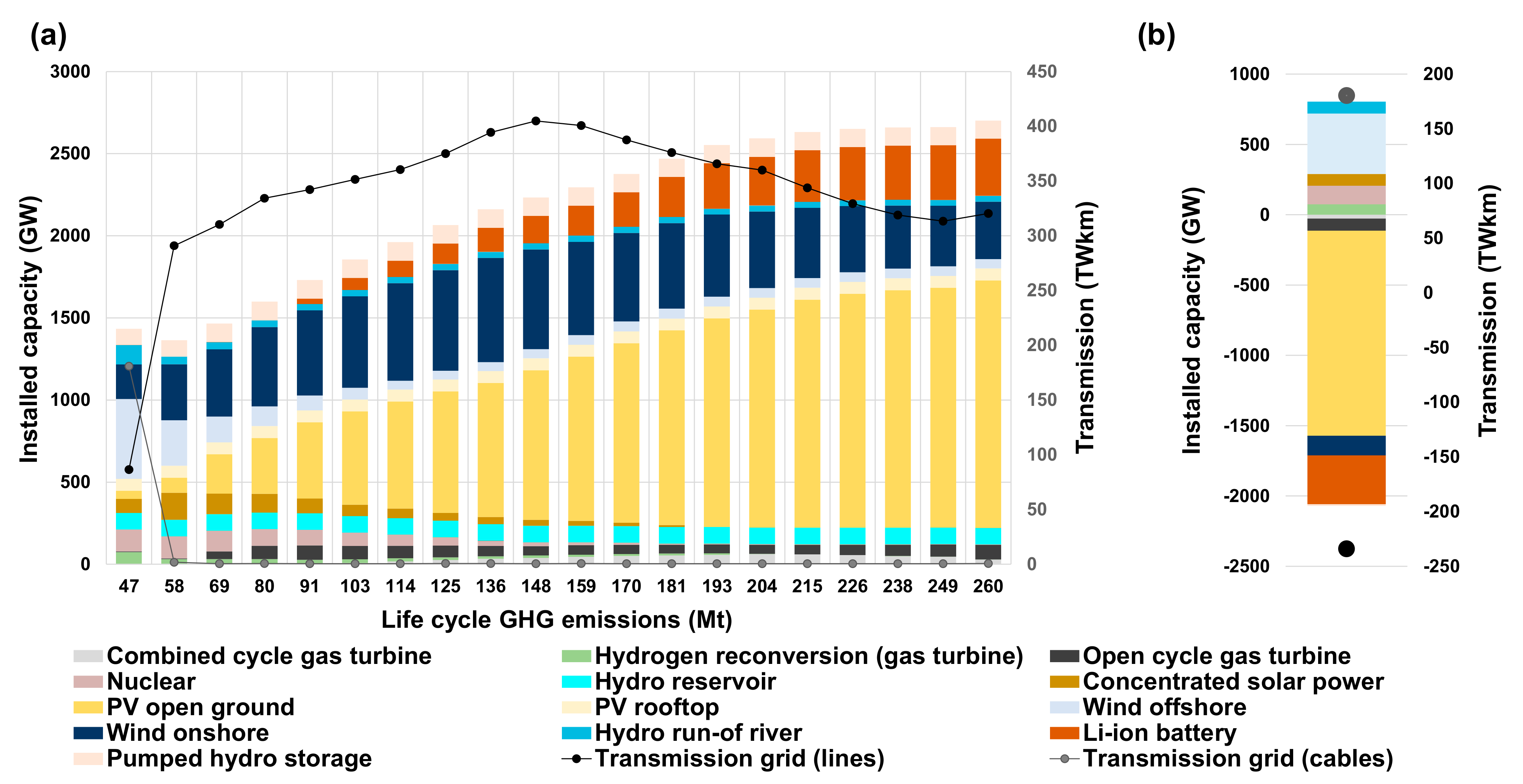
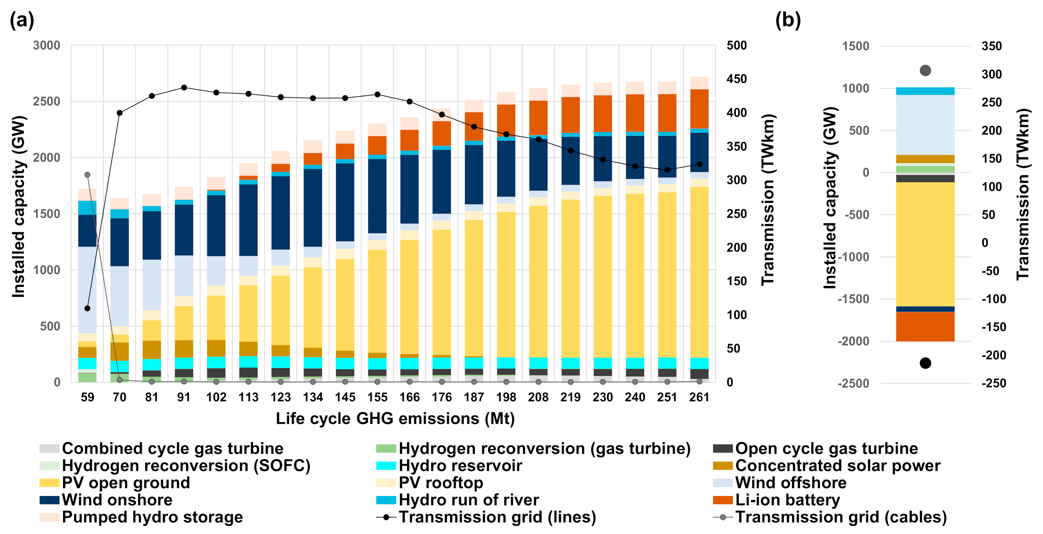
Figure 4 shows the power generation capacities in panel (a) and the difference between the two extremes, the cost optimum, and the least GHG emissions intensive solution, are shown in panel (b).
As shown in panel (a), the cost-optimal power system (outer right bars) is dominated by PV open ground and wind onshore. Temporal flexibility is mainly provided by Li-ion batteries and pumped hydro storage, while the grid is expanded to ~320 TWkm, which is in the range of grid expansion needs shown in earlier work with comparable scenario setups [
21,
36]. Additional flexibility to the system is provided by a small share of combined and open cycle gas turbines. As shown
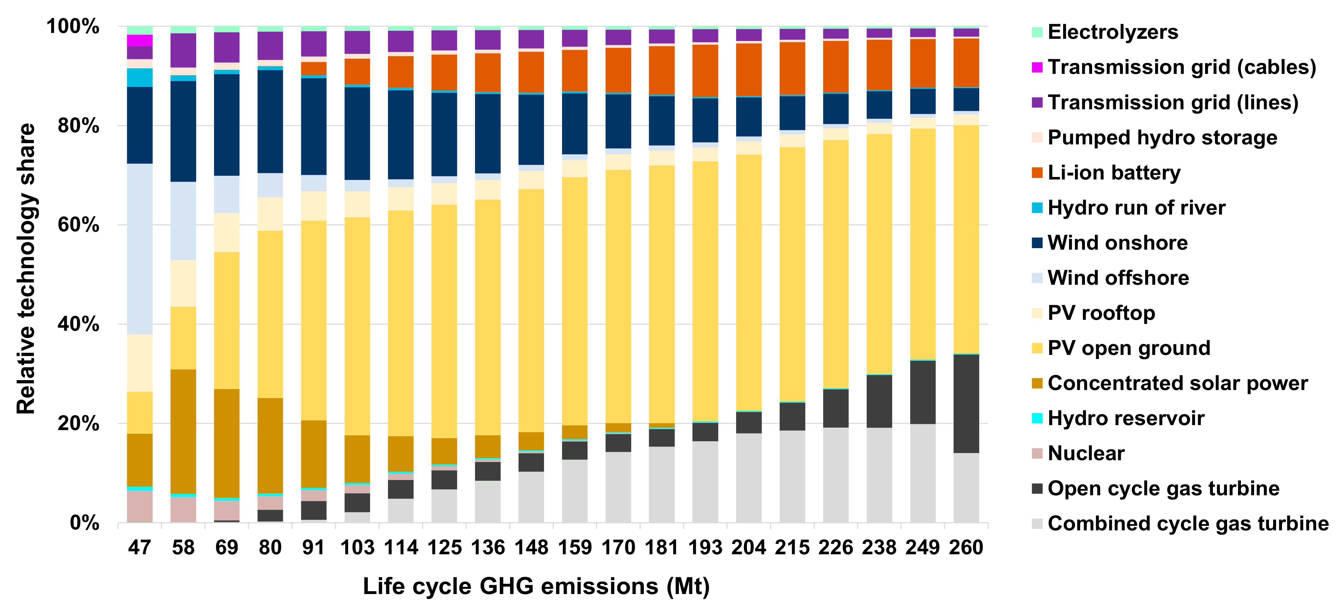
Figure 5, life cycle GHG emissions in the cost-optimal system are dominated by PV open ground and gas power plants. For PV, upstream industrial (e.g., flat glass production) and transport processes are responsible for most of the GHG emissions, whereas direct combustion emissions dominate the impact for gas turbines.
The first 22% of the reduction of life cycle GHG emissions (from 260 to 204 Mt) is achieved through an expansion of wind onshore and grid, while the share of PV open ground systems and Li-ion batteries is reduced. The correlation between the expansion of the grid with an increasing share of wind power when dispatchable generation is limited has been shown in earlier work [
27] and can be observed until life cycle GHG emissions are reduced to 148 Mt, where the grid expansion reaches a maximum. In addition, the decline of Li-ion battery storage with the reduction of life cycle GHG emissions contributes to the increasing need for power transmission. Thus, a co-expansion of the grid and wind power can be considered a viable option for a cost-effective reduction of life cycle GHG emissions. At 148 Mt life cycle GHG emissions, the system is balanced between PV and wind onshore with small shares of conventional power plants and CSP to provide dispatchable generation. Life cycle GHG emissions are still dominated by PV open ground (
Figure 5).
The need for grid expansion and storage, however, decreases when increasing shares of CSP and nuclear enter the system to further reduce emissions. Until life cycle GHG emissions are reduced to 69 Mt, open cycle gas turbines are operated at low capacity factors (<0.01) to meet demand at peak load hours. VREs still make up a considerable share in the overall power plant portfolio with offshore wind becoming a more dominant source of power supply, as it is associated with higher capacity factors and less specific life cycle GHG emissions per unit of electricity supplied than onshore wind power plants and PV. A reduction of emissions to 58 Mt is accompanied by an increasing share of CSP, wind offshore, with nuclear being deployed to its full capacity (~131 GW) and operating with a high capacity factor (>0.9). At this stage, total life cycle GHG emissions are no longer dominated by PV technologies but CSP and wind on- and offshore. Moreover, direct emissions are fully mitigated as gas turbines are no longer operated to cover demand in peak load hours.
The system that is the least GHG emission intensive is characterized by a large share of wind off- and onshore, hydro run of river, CSP, and nuclear capacities (
Figure 4). As the share of CSP is reduced compared to the previous three solutions, hydrogen reconversion provides additional temporal flexibility to the system. In addition, this is the only system in which electricity transmission is based on copper-based cables that are more climate friendly than aerial lines that rely on aluminum as a conductor. The significantly higher costs of cables compared to aerial lines, however, leads to the deployment of this technology only in the least emission intensive solution. Total grid transfer capacity is almost as high as in the cost-optimal solution.
Along the pareto front, the total installed capacity is increasingly reduced. Comparing the two extremes, the cost optimum and the least emission-intensive solution in panel (b) of
Figure 4, the reduction of life cycle GHG emissions to the minimum results in systems with technologies that are characterized by higher capacity factors and lower GHG emissions per power output than the technologies deployed in the cost-optimal solution. Although the high share of wind offshore is associated with considerable need for a transmission grid for geographical load balancing, the total grid demand is lower than in the cost optimum.
In summary, it is possible to achieve power systems that are both affordable and sustainable in terms of reducing life cycle GHG emissions. In this respect, PV is still the dominant technology, but with a higher importance of wind onshore and the expansion of grid transmission capacity compared to the cost minimal system. Further reductions in life cycle GHG emissions can be achieved through the increased expansion of dispatchable generation but are accompanied by higher increases in system costs. However, for a comprehensive assessment of life cycle environmental sustainability, a multitude of indicators needs to be analyzed. Therefore, in the following section, we perform an ex-post assessment of the energy systems presented above using the indicators listed in
Table 1.
3.3. Environmental Ex-Post Assessment
In this section, the co-benefits and adverse side-effects of the reduction of life cycle GHG emissions are analyzed with respect to indicators listed in
Table 1. This ex-post assessment of environmental impacts is based on the solutions on the pareto frontier shown above.
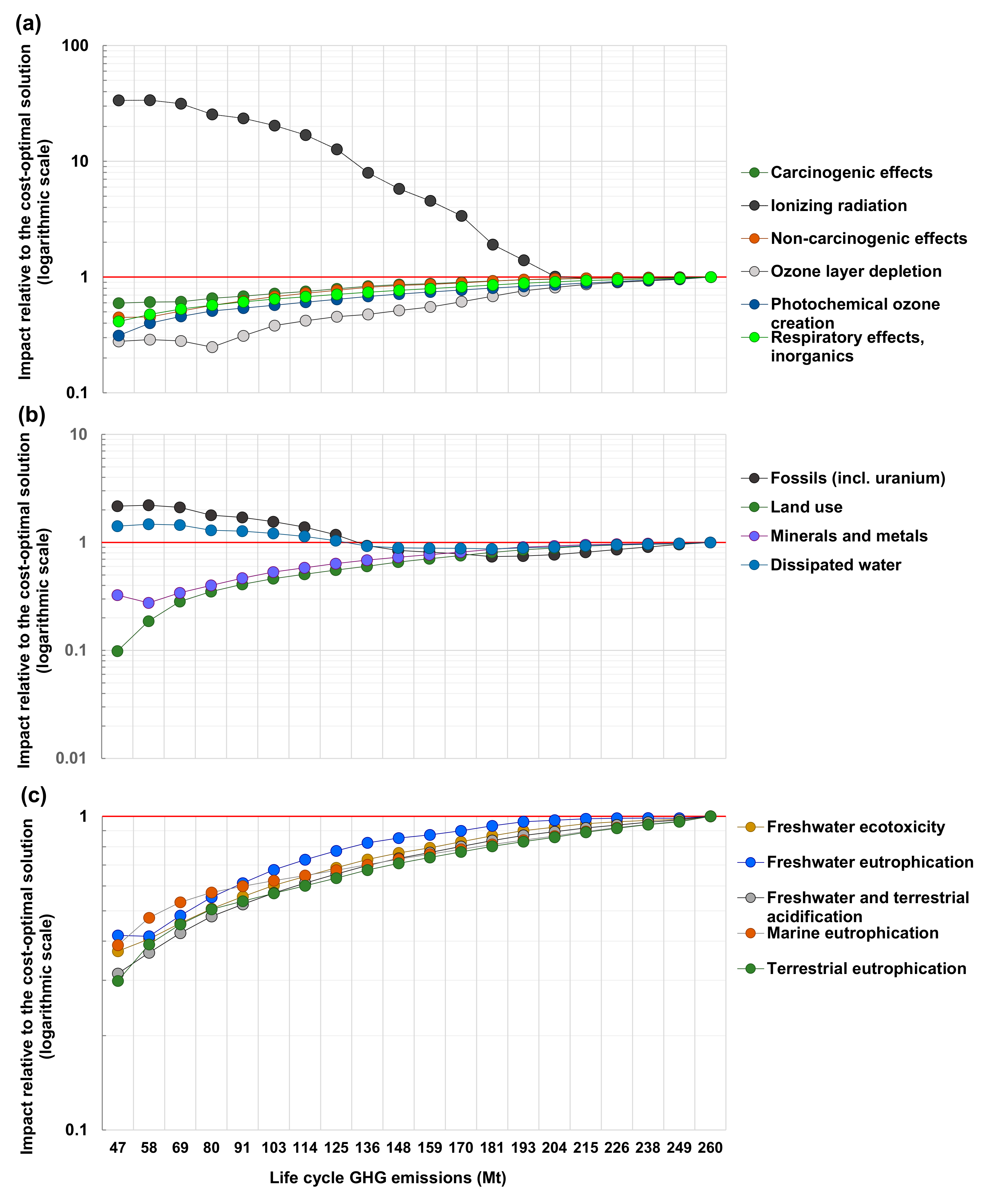
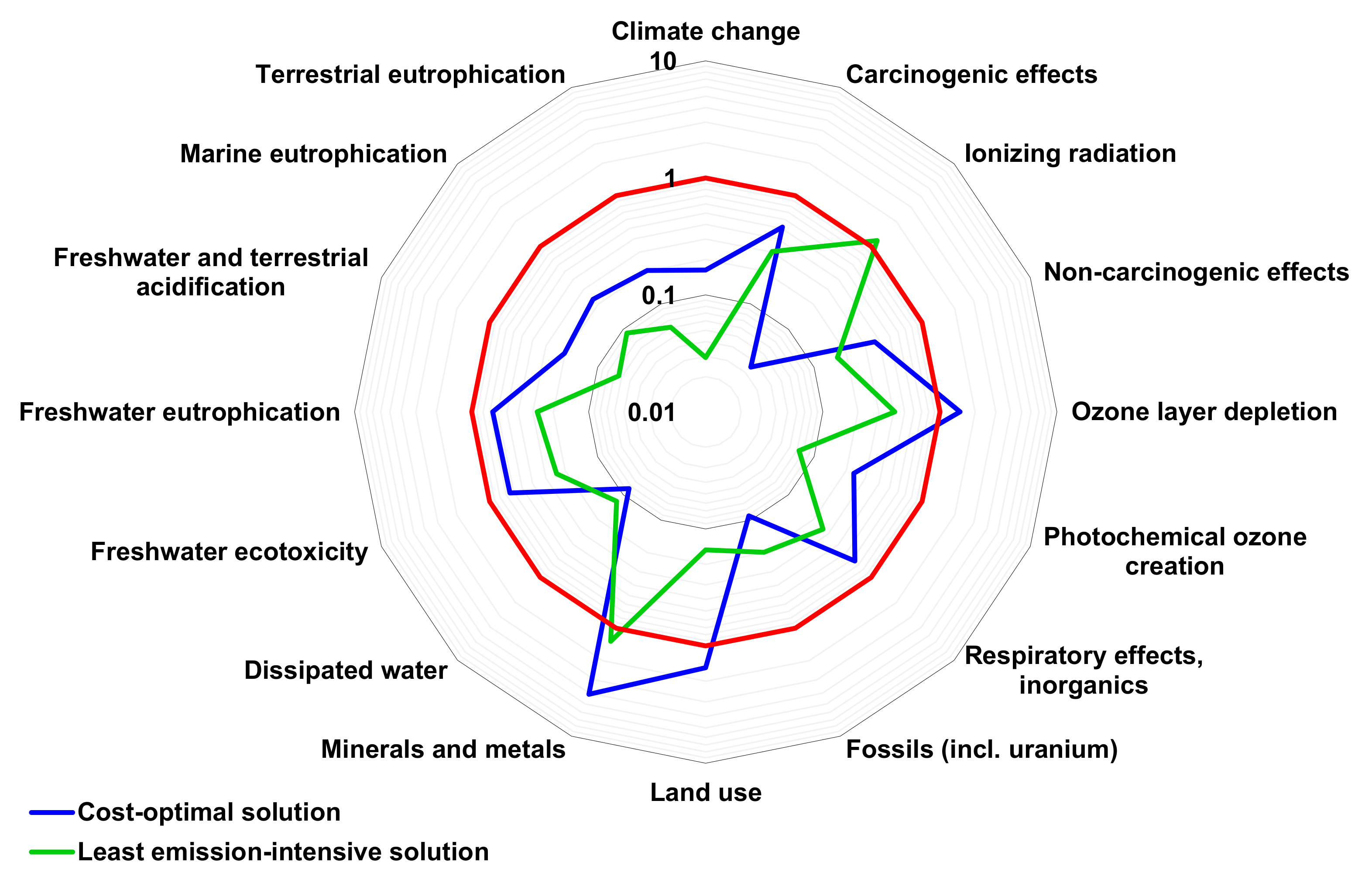
Figure 6 illustrates the evolution of life cycle metrics for the different areas of protection over the pareto front.
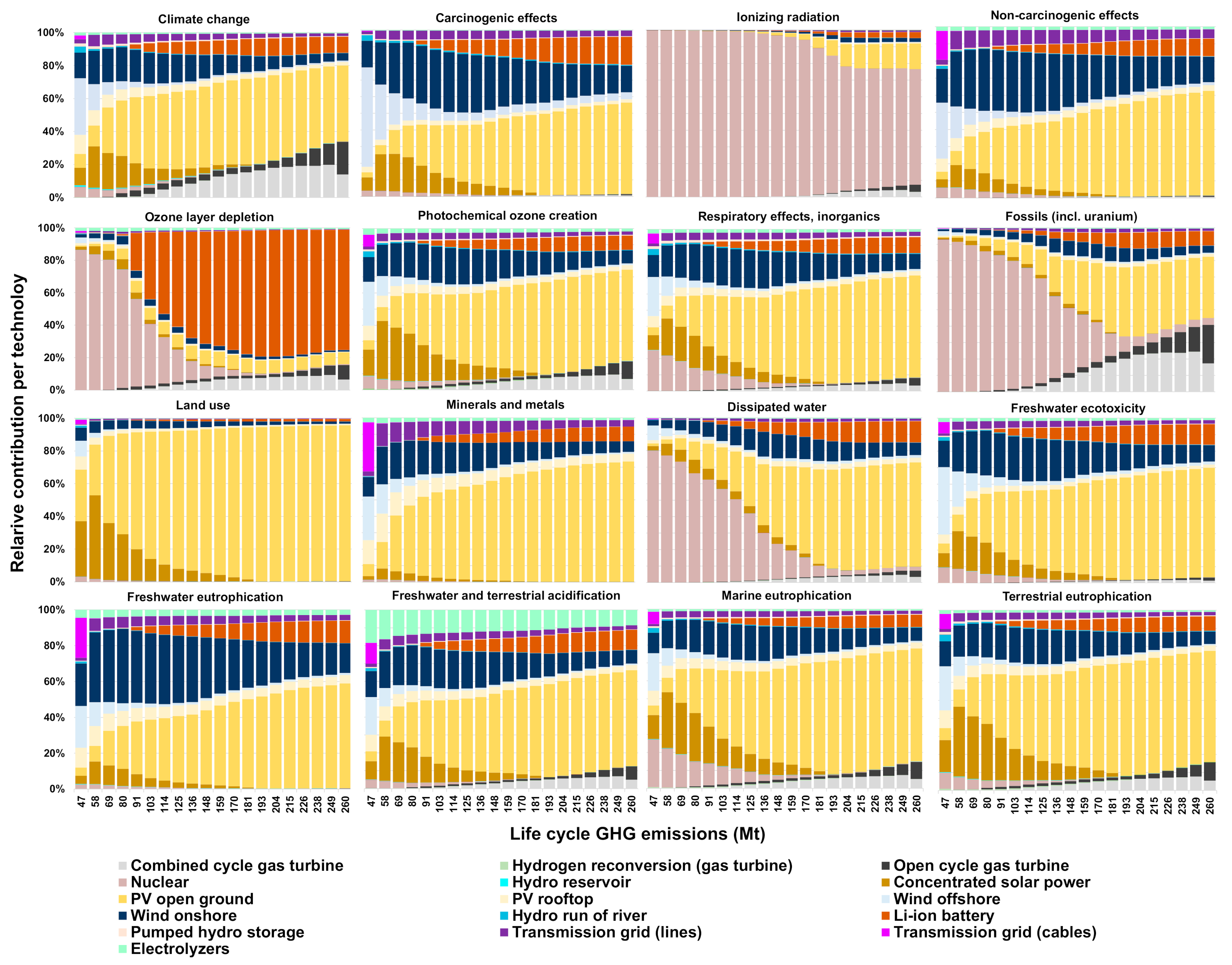
The majority of indicators show co-benefits with reduced life cycle GHG emissions. Only three impact categories increase with the reduction of life cycle GHG emissions. The co-benefits are mainly induced by the decreasing deployment of PV open ground installations, since this technology dominates nearly all impact categories in the cost-optimal system (see the relative share of technologies for each impact category in
Figure A1 in
Appendix C). Onshore and offshore wind show the highest impacts for the least GHG-emitting system in most categories. The increase in nuclear power is responsible for adverse side-effects.
The strongest adverse side-effect on human health (panel (a)) results from exposure to ionizing radiation caused by nuclear energy, which increases with its use (up to a factor of ~34 compared to the cost-optimal solution). With the exception of ozone depletion, most other indicators show clear trends with decreasing climate impacts. At a reduction of life cycle GHG emissions to 80 Mt, ozone layer depletion reaches its minimum. At this point, Li-ion battery storage leaves the system, after dominating this indicator in the previous solutions, and the main driver becomes nuclear power plants. The use of nuclear energy is associated with ozone depleting emissions of halogenated hydrocarbons for cooling during uranium production. The development of impacts over the pareto front related to resource depletion are shown in panel (b). Down to 136 Mt GHG emissions we see co-benefits related to reduction of climate impacts. For fossils (including uranium) and dissipated water, they turn into adverse side-effects with further emission reduction. In the cost-optimal system, the use of fossils is dominated by electricity generation with gas turbines and the construction of PV plants. As life cycle GHG emissions are reduced, fossils and water depletion become dominated by nuclear power. For nuclear power, cooling water has a high impact on water depletion. Both, PV and CSP have a high direct land demand. CSP accounts for nearly half of the land use when installed capacity peaks at the reduction of life cycle GHG emissions to 58 Mt. A further avoidance of life cycle GHG emissions from 58 Mt to 47 Mt results in a slight increase in minerals and metals as wind offshore and copper-based cables are deployed where the metals used have a higher depletion potential compared to metals used for CSP and aluminum-based aerial lines. The development of impacts over the pareto frontier related to ecosystem quality are shown in panel (c). For all these indicators, we see co-benefits associated with reducing climate impacts. In this group, the contributions of the individual technologies show a similar pattern to that of climate change. Only the electrolyzers have a higher contribution to freshwater and terrestrial acidification, while gas turbines have a lower impact, especially in freshwater ecotoxicity and freshwater eutrophication. As with minerals and metals, the use of transmission cables overcompensates for the reduction in freshwater eutrophication achieved by decreasing PV deployment. Again, the higher impact of copper production is responsible for the increase.
The high share of PV in most impact categories is also consistent with findings by Berrill et al. [
6], who conducted an LCA of 44 electricity scenarios for Europe in 2016. The authors showed that wind-dominated systems have half as much life cycle GHG emissions as PV-based systems. Moreover, they found that PV-based systems have a higher environmental impact on indicators that affect human health and ecosystems than wind-dominated systems.
Carcinogenic, non-carcinogenic, and respiratory effects show the lowest reduction over the pareto front. This means that they are least sensitive to the technological changes. Most sensible are ionizing radiation, fossils, and dissipated water, although these changes are only due to the expansion and operation of nuclear power.
As illustrated in
Figure A2, compared to today’s impacts of power supply, land use is likely to increase should the power system have a high share of PV open ground. A similar increase compared to today could be expected in ozone layer depletion in case the system has high shares of Li-ion batteries. Moreover, all systems analyzed in this study could result in higher depletion potential for minerals and metals compared to today’s values. Current levels in ionizing radiation could be exceeded if nuclear energy is largely deployed.
4. Discussion
In this section, we first summarize our findings and derive the main implications. We then examine the role of nuclear power and provide an outlook based on the identified needs for further research.
4.1. Summary and Implications of the Results
In this study, the ESOM REMix is populated with environmental impacts of the entire supply chain of the considered technologies, which is achieved through coupling with the elaborated LCA-framework FRITS. Hereby, to the best of our knowledge, we conduct the first integration of LCA impacts in an ESOM with high spatiotemporal detail. This enables a comprehensive assessment of the trade-offs of life cycle GHG emissions and system costs of the electricity sector in EUNA combining the strengths of energy system modeling and LCA approaches. Furthermore, the comprehensive nature of the methodology provides information on a large set of additional environmental co-benefits and adverse side effects, highlighting potential areas of conflict between an increasingly climate friendly electricity supply and other life cycle impact categories.
The results underline the fact that the most cost-effective decarbonization of the power sector in EUNA leads to emissions that are largely generated in the upstream supply chain. A reduction of life cycle GHG emissions, which includes all emissions (direct and indirect), strongly reduces direct CO
2 emissions, thereby increasing the relative importance of upstream emissions. Moreover, our results show that different low-carbon power supply options are not equally effective. Rather, they differ significantly in terms of life cycle GHG emissions, with the result that a reduction in these emissions relies increasingly on wind, CSP, and nuclear with moderate variations in grid expansion. At the same time, the share of PV and Li-ion storage is declining. A study that confirms these observations was published by Pehl et al. [
15]. It had a global focus and showed that a tax of USD 30 per ton of life cycle GHG emissions leads to an energy system with a larger share of wind power, CSP, and nuclear power compared to a system with a tax on direct GHG emissions only, underlining the life cycle GHG emission benefits of these technologies. However, since the authors did not perform multi-objective optimization covering the entire solution space of possible system configurations, our study also shows extreme solutions with higher deployment of technologies favorable for reducing life cycle GHG emissions.
This study focuses exclusively on very ambitious systems regarding the avoidance of direct CO
2 emissions. It is therefore important to note that even if decarbonization of the power sector follows cost optimality, life cycle GHG emissions can be expected to be low compared to today’s levels (see
Figure A2).
4.2. The Role of Nuclear Power Generation
Our analysis shows that the reduction of life cycle GHG emissions largely increases ionizing radiation, water consumption and depletion of fossils (particularly uranium) due to the expansion of nuclear power. The deployment of nuclear to reduce life cycle GHG emissions also raises several other concerns not captured in LCAs, such as the risk of severe accidents, risks to the environment and local communities and the storage and treatment of nuclear waste. Furthermore, Kim et al. [
47] showed that the degree of public acceptance of nuclear power in European countries is highly dependent on perceived potential risks, which could hinder the continuation of nuclear based electricity generation through social opposition (e.g., in case of an accident). In this context, we additionally conducted REMix calculations without nuclear energy (see
Figure 7). Corresponding figures regarding the pareto frontier and the development of the other environmental indicators can be found in the
Supplementary Materials.
This results in a reduction in the life cycle GHG emissions of up to 59 Mt with a simultaneous cost increase to EUR 415 billion (
Figure S1). Such a system is dominated by wind and CSP and accompanied with higher grid expansion and hydrogen re-conversion for regional and temporal load balancing compared to a system with nuclear power. Furthermore, systems without nuclear power only show co-benefits with regard to other environmental impacts with decreasing life cycle GHG emissions (see
Figure S2).
4.3. Life Cycle Data Must Become Prospective
This study encounters methodological limitations that need to be considered when interpreting the results.
First, the LCIs are not fully prospective with respect to the fore- and background processes. For example, fossil-based process heat is responsible for a high share of the life cycle impacts of PV. To better understand how these emissions can be reduced in the future, a comprehensive understanding of potential decarbonization measures in the upstream supply chain of energy technologies and the corresponding integration into life cycle databases is necessary. Fully decarbonized industrial and transportation processes could largely reduce the upstream emissions and have a significant impact on the results. Combined with prospective foreground LCIs, this could also strengthen the role of PV in reducing life cycle emissions of ambitious energy systems in future studies. It should be noted, however, that relative differences between technologies are decisive in optimization. Thus, if PV does not improve relative to the other technologies when adjustments are made to fore- and background LCI data, it can be assumed that the technology mix will remain similar as shown here and only the absolute level of environmental impact would be affected.
Second, the classification of technologies for which LCI data are available is not necessarily identical with the rather general classification in the ESOM. For this purpose, we selected representative technologies from the available LCI data and, in the case of PV, relied on sub-technology compositions to capture different technological characteristics. However, future efforts are required to better align the ESOM technology classification with the LCIs on energy technologies. Coping with all these challenges, however, involves uncertain impacts across the different life cycle phases and requires a significant modeling effort, which in turn calls for joint community action.
4.4. Outlook
Our modeling approach should be used to include further indicators to aim for completeness from the perspective of sustainability, such as societal aspects and other economic and environmental impacts of the energy transition [
48]. Options for performing such analyses could include either multi-objective optimization considering a variety of conflicting objectives or ex-post assessment. Parallelizing the
ε-CM as performed here could keep computation time manageable when extending the optimization approach to other indicators and more dimensions. However, the calculation of social and economic indicators requires more specific modeling approaches as they are currently not sufficiently covered by LCA.
When interpreting the results of the present study, the limited sectoral resolution must be considered. For example, the expansion and operation of technologies in the heat and transport sectors are not included. Vandepaer et al. [
18] used a multi-sectoral ESOM for Switzerland and showed, for instance, that in an energy system optimized towards life cycle GHG emissions, additional power generation capacity is added to deploy a higher proportion of hydrogen-based transportation technologies compared to the cost-optimal solution where transportation is mostly based on battery electric vehicles. Therefore, the sectoral extension of the approach presented in our study is crucial to fully understand the impact of considering life cycle GHG emissions on the structure and overall environmental performance of the entire energy system.
5. Conclusions
In this study, we included life cycle environmental impacts in the highly resolved ESOM REMix applied for the assessment of infrastructural demand in low-carbon scenarios. We thereby extended the usually cost-oriented nature of such analyses. The ESOM was applied to assess future configurations of the power system in Europe and North Africa that aims to reduce direct CO2 emissions by at least 95% compared to 1990. Within this ambitious system, life cycle GHG emissions were considered in the optimization and systematically reduced to the feasible minimum. Moreover, we provided further insights by quantifying other life cycle impacts associated with the different system configurations (such as land use, minerals and metals, carcinogenic effects and other impacts). In this way, co-benefits as well as adverse side effects for fifteen mid-point indicators that come along with a reduction of climate impacts were assessed using the ILCD 2.0 2018 impact assessment methodology.
The first half of possible life cycle GHG emission avoidance can be achieved with comparably small increases in total system costs (compared to the cost-optimal solution for a 95% reduction in direct CO2 emissions), while a reduction of the last half considerably increases the system costs. Systems where life cycle GHG emissions are reduced at moderate costs increasingly rely upon on- and offshore wind power, grid expansion with reduced shares of Li-ion batteries and PV. Thereby, the deployment of wind turbines and PV panels contribute to the climate impact of electricity generation with up to 70%. The increasing reduction of life cycle GHG emissions is supported by the deployment of wind offshore, CSP and nuclear power. Nuclear operates as a base-load power plant with high capacity factors (>0.9). However, such systems are associated with considerable cost increases (by up to 63% compared to the minimum cost solution). As life cycle GHG emissions are reduced, hydrogen re-conversion is used to cover demand in peak load hours.
This research contributes to a better understanding of trends in environmental impact categories other than climate change (e.g., land use). The impacts in most categories are improved in the reduction of life cycle GHG, i.e., they show co-benefits. Considering the increasing deployment of nuclear power plants which represents an option to reduce the effects of climate change, it also affects other categories such as ionizing radiation, fossils (including uranium) and water use negatively. Moreover, other impacts related to nuclear power and not included in LCA such as the risk of an accident, waste treatment and social acceptance were outside the scope of our assessment. In an additional model calculation, we illustrated that high reductions in life cycle GHG emissions are also possible without nuclear power. Here, grid expansion for regional load balancing is more important than in a system with nuclear power. Moreover, all life cycle indicators improve compared to the cost-optimal system.
In summary, the combination of LCA and ESOMs is of great benefit to both methods. Integrated assessments of future energy systems and their impacts on sustainability are expected to become more important due to pending developments in the energy system, such as renewable electrification of transportation, heat and other sectors. Moreover, global supply chains linked to the world’s energy system are becoming increasingly complex and energy system transformations are evolving at different speeds across regions. Informed decisions on the design of the future energy system therefore require the consideration of impacts upstream in the supply chain to avoid major burden shifts.
A potential policy implication from our work is that life cycle impacts of energy technologies should be considered in the future design of policy instruments, as emissions are increasingly shifted upstream in an ambitious energy system. However, current approaches that combine both modeling worlds in an integrative approach still face several limitations, such as missing aspects regarding prospectivity and high uncertainties of LCI data and should remain a priority research area in the future. This study should therefore be regarded as a further step towards integrated model-based assessment and confirms the call for joint work between researchers in the field of energy system modeling and industrial ecology. For example, it would be of great benefit to develop a system in which a centralized, collaboratively developed, and prospective LCI database is used as a reference with defined criteria to map LCI data to processes in the ESOMs.


