Design Framework for Achieving Guarantees with Learning-Based Observers

Abstract

The paper proposes a novel framework for state observer design, in which learning-based observers are incorporated. The aim of the method is to provide a framework, which is able to guarantee the limitation of the observation error, even if the error of the learning-based observer under all scenarios cannot be verified. The framework is based on the robust ${\mathcal{H}}_{\infty }$ design method, which is able to provide guarantees on the resulted observer. Moreover, the observer design process is extended with a controller design, which leads to a joint robust ${\mathcal{H}}_{\infty }$ controller-observer design. In this paper the proposed method is applied on a vehicle control problem, such as lateral path following. In this problem the goal of the observer is to provide an accurate lateral velocity signal for the vehicle, which is used in the controlled system for the generation of front wheel steering angle. The effectiveness of the method is illustrated through simulation examples on high-fidelity vehicle dynamic simulator CarMaker.

1. Introduction and Motivation

The development of the complex automatic control systems has become a high challenge for the industry. One of the most important field is the control of autonomous vehicles, in which various safety performance requirements and similarly, enhanced functionality for the vehicle systems must be guaranteed. It requires lots of measurements using high number of sensors. During the sensing process in the industrial applications, several states of a given system can be measured, which play a crucial role in the control system. In many cases, not all of the states of a system can be measured directly or the appropriate sensors are too expensive for wide use. However, the increasing number of achievable signals makes possible to observe, estimate and predict the states of the system, which can lead to enhanced functionality in the controlled system.

Several approaches have been developed for the observation problems in recent years. In terms of solutions, two main groups can be distinguished. In the first group, the classical approaches can be found. In [1] a gain scheduled ${\mathcal{H}}_{\infty }$ observer can be found, in which the time delays and the saturation of the actuator are taken into account. An ${\mathcal{H}}_{\infty }$ filtering method for the problem of state of charge and state of health monitoring in electric vehicles is used in [2]. Orientation angles are determined using nonlinear Luenberger observer in [3], during the estimation process low-cost inertial measurement unit is used. Moreover, in [4] a method is proposed for minimizing the disturbances and the errors of the estimation by using ${\mathcal{H}}_{\infty }$ norm approach. Furthermore, a polytopic system-based solution is presented in [5]. The goal of that paper is to solve the state estimation and the fault detection problem at the same time. The work of [6] describes a control method for linear parameter varying systems using a polytopic observer. Although the proposed methods are able to handle the nonlinearities of the system, they require the accurate knowledge of the observed system. In many cases the nonlinearities of the system unknown. Methods based on big data analyses can be used in order to improve the accuracy of the estimation process.

In the second group, the non-conventional methods can be found. In these methods the estimation process is extended with the results of the machine learning algorithms, with which the accuracy can be increased especially in nonlinear operation range. In [7] the estimation is an essential part of the control system of an induction motor, which applies a neural network-based solution. Furthermore, machine learning-based observers can also be used for mobile robots, see [8]. However, these approaches cannot provide analytical guarantees for the performances of the estimation. Using the combination of the neural network results and a model-based estimation approach, the performances can be increased significantly. For example, a Luenberger observer is extended with the results of the neural network in [9]. A solution for the estimation of the motor inertia value is presented in [10]. The inertia value is observed using a extended Luenberger observer, in which the gain matrix of the observer is adjusted using a neural network. Moreover, in [11] a ${\mathcal{H}}_{\infty }$ filtering algorithm is combined with the results of neural network in order to measure the rolling angle of the vehicle. In the proposed solution only the on-board sensor signals are used and the method is based on a sample vehicle model. Kalman filtering is another important approach in the problem of state estimation with lots of practical implementation possibilities. For example, [12] proposes a cascaded Kalman filtering method for state estimation in the field of cooperative lateral vehicle following. In the context of electric vehicles, Kalman filtering can be used for the state estimation of the batteries [13]. Through an appropriate method the real-time operation of the filtering process can be guaranteed [14].

The benefit of the classical approaches is that they are able to provide provable guarantees on the observation. For example, in case of model-based observer design process it is possible to scale the maximum error of the process, i.e., the difference between the estimated and the real signal. Nevertheless, it requires the accurate model on the system and the achievable observation performance due to the limited complexity of the model is limited. Despite, the learning-based observers has the advantage to provide accurate observation while preliminary physical model on the process is not required. The design of the observer is based on a training process, in which several scenarios are used, e.g., in a supervised learning or in a reinforcement learning process. Since it can be difficult to formulated some type of nonlinear dynamics of the system, an advantage of the learning-based approach is that their effect on the performances can be catched through learning. Thus, it is unnecessary to use complex nonlinear identification methods to achieve a control-oriented state-space model. Furthermore, an advantage of the learning-based observers is that high number of measured signals for achieving an accurate observation can be used, especially the inputs of the agent can contain unstructured data (e.g., camera frames). Although learning-based techniques has high effectiveness in practical applications, it is difficult to provide provable guarantees on the performance level of the observation process.

The aim of this paper is to propose a framework for the design of observers, in which the model-based and the learning-based approaches are integrated. The goal of the paper is to bridge the gap between the observer design methods, i.e., provide guarantees on the minimum performance level of the observation process, and similarly, provide the possibility for improving the maximum performance level simultaneously. The role of the model-based observer is to provide an observation, which has guarantee on the minimum performance level. The aim of the learning-based observer is to provide another observation, which is potentially more accurate. The output of the learning-based observer is taken part in the model-based observer to improve the final observation signal. The contribution of the paper is a design framework with the model-based observer design, in which some information on the learning-based observer is incorporated in. The advantage of the method is that it is independent on the internal structure of the learning-based observer, and thus, it can be used providing guarantees for various agents. In this paper the proposed framework is applied to an observation problem in the field of the vehicle control, i.e., lateral path following.

The paper is organized as follows. The design framework and the concept behind the observation is presented in Section 2. The design of the model-based observer with the consideration of the learning-based observer is presented. Section 4 presents the application of the proposed method to a vehicle control problem and moreover, simulation results for the illustration of the observation effectiveness is also presented. Finally, in Section 5 the conclusions of the paper and the further challenges are summarized.

2. Design Framework

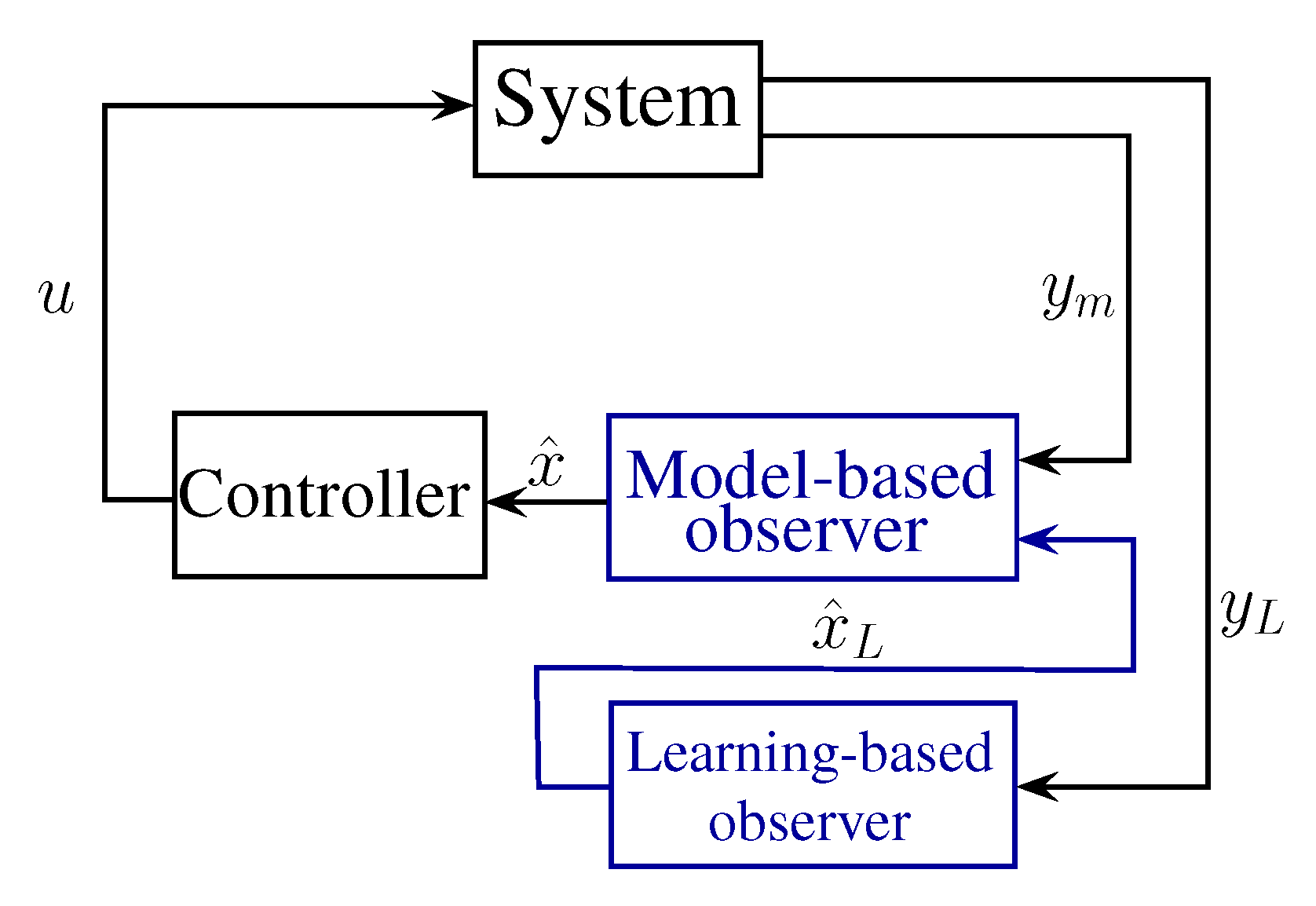
In this section the framework for the observer design is presented. The structure of the observer, together with a controller is illustrated in Figure 1.

The idea behind the framework is to provide $\widehat{x}$, which is as close as possible to the real state vector x of the system. Since in various industrial applications the observer is used for control purposes, $\widehat{x}$ can be used for the generation of control input u through the controller $u=K(\widehat{x})$. Nevertheless, the design of the observer is independent from the control design, and thus, $\widehat{x}$ can be used for non-control purposes, e.g., monitoring the operation of the system.

In the design framework it is considered that the input of the model-based observer and the input of the learning-based observer can be different, i.e., it is not necessary that the measurements $y_m$ and $y_L$ to be the same. Generally, the learning-based observers can use high number of measured signals, due to their complex and nonlinear structure. For example, in case of environment sensing applications the estimation of the autonomous vehicle position on the road is based on camera information, which can be considered as unstructured data. Despite, the model-based observers has a structure with limited complexity and thus, the number of the measured signals are also limited. Moreover, in case of model-based observers structured data can be used in the process. Therefore, it is advantageous to differentiate $y_m$ and $y_L$, but the measured signals in $y_m$ can be the parts of $y_L$.

The output of the learning-based observer is noted with ${\widehat{x}}_L$, which is the estimation on the state vector of the system. This information is used by the model-based observer to improve the estimation $\dot{x}$, with which $|x-\widehat{x}|$ is minimized. The idea is close to the concept of the Kalman-filtering, in which innovation term is used to update the model-based estimation. In the update process of the Kalman-filtering it is considered that the measurement for the innovation is accurate, and thus, the estimation is fitted to that. Despite, in the proposed concept ${\widehat{x}}_L$ is considered to be accurate in most cases, but not necessarily in all scenarios. For example, there can be scenarios, when the output of the learning-based observer is highly inaccurate, such as faults or rare inputs, which are highly different from the samples in the training set. The goal of the proposed observer structure is to avoid the unlimited increase of inaccuracy in the observation, i.e., the limitation of the error between x and $\widehat{x}$ must be guaranteed. It is achieved through the model-based observer design, which provides the minimum performance level of the observer, i.e., bounds on the observation error. Nevertheless, the learning-based observer is considered to be designed on a way that it is able to provide accurate observation under normal circumstances and thus, the consideration of ${\widehat{x}}_L$ has benefits on the minimization of the error $|x-\widehat{x}|$. It results in the improvement of the observer maximum performance level. Decision on the accuracy of ${\widehat{x}}_L$ is the part of the operation of the model-based observer, whose design is detailed in the following section.

3. Robust Design of the Model-Based Observer

The goal of this section is to propose the design of the model-based observer, in which the output ${\widehat{x}}_L$ of the learning-based observer is incorporated. The model-based observer design is based on the robust ${\mathcal{H}}_{\infty }$ method, with which guarantee on the error of the observation can be provided. Moreover, in this section the design of the observer is extended with the design of a robust controller for closed-loop purposes, which results in an output-feedback ${\mathcal{H}}_{\infty }$ controller with guarantees.

The designed model-based observer must guarantee the following features.

• The model-based observer must provide an observation $\widehat{x}$, with which the observation error ${(x-\widehat{x})}^2$ is minimized. It requests an accurate model on the process, and on the measurement $y_m$. Moreover, the observation is improved through ${\widehat{x}}_L$.
• The model-based observer must decide on the acceptability of ${\widehat{x}}_L$. Its reason is that the learning-based observation process can degrade, because the performance level on the observation is not guaranteed. For example, ${\widehat{x}}_L$ is unacceptable if there are faults in the operation of the learning-based agent. Another example is that if an input sample for the agent significantly differs from the samples in the training set and thus, ${\widehat{x}}_L$ can lead to a reduced performance level. This feature through the robust design is achieved.

The model for the observer design is based on the state-space representation

$$\begin{array}{cc}\hfill \dot{x}& =Ax+B_{2}u,\hfill \end{array}$$

(1a)

$$\begin{array}{cc}\hfill y_m& =C_{2}x;\hfill \end{array}$$

(1b)

where $A,B_2,C_2$ are matrices, x represents the state vector of the system with n states and u is the control input. for simplicity, one control input is considered in the rest of the paper. Moreover, the signal ${\widehat{x}}_L$ is considered as a bounded disturbance in the system. In spite of the classical disturbance signals, ${\widehat{x}}_L$ has benefits on the system in most cases, as presented in Section 2. During the design of the model-based observer, it is requested that the observation of the learning-based observer must be inside of a bounded range of the model-based observation. And thus, the model-based observer must be robust against the bounded disturbance. Consequently, the maximum observation error, i.e., the minimum performance level of the observer is guaranteed by the ${\mathcal{H}}_{\infty }$ design.

The goal of the observer is to minimize the difference between the states of the system and the estimated states, such as

$$\begin{array}{c}\hfill \underset{t\to \infty }{lim}{(x(t)-\widehat{x}(t))}^2\to min.\end{array}$$

(2)

Thus, it is requested to find an observer matrix L which is able to minimize the objective (2). The structure of the observer, which contains L and the model of the systems is formed as

$$\begin{array}{cc}\hfill \dot{\widehat{x}}& =A(\widehat{x}+\mathsf{\Delta })+B_{2}u+L(y_m-C_2\widehat{x}),\hfill \end{array}$$

(3)

where $\mathsf{\Delta }$ vector is the improvement based on the learning-based estimation ${\widehat{x}}_L$. The values in $\mathsf{\Delta }$ is formed as follows. The values in $\mathsf{\Delta }={[{\mathsf{\Delta }}_1\dots {\mathsf{\Delta }}_i\dots {\mathsf{\Delta }}_n]}^T$ are bounded by predefined values ${\mathsf{\Delta }}_{min,i},{\mathsf{\Delta }}_{max,i}$, such as

$$\begin{array}{c}\hfill {\mathsf{\Delta }}_i=max\left(min\left({\widehat{x}}_i-{\widehat{x}}_{L,i};{\mathsf{\Delta }}_{max,i}\right);{\mathsf{\Delta }}_{min,i}\right),\forall i\in n,\end{array}$$

(4)

where $max,min$ functionals represent the selection of the higher or lower values and index i for ${\widehat{x}}_{L,i},{\widehat{x}}_i$ represents the elements of the state vector. It means that $\mathsf{\Delta }$ can be interpreted as a state correction from ${\widehat{x}}_L$, which is bounded to avoid the degradation of $\widehat{x}$, if ${\widehat{x}}_L$ is degraded. (4) expresses that ${\widehat{x}}_i-{\widehat{x}}_{L,i}$ must be between ${\mathsf{\Delta }}_{min,i}$ and ${\mathsf{\Delta }}_{max,i}$. The selection of ${\mathsf{\Delta }}_{min,i}$, ${\mathsf{\Delta }}_{max,i}$ depends on the requirements on the acceptable maximum observation error, i.e., if ${\widehat{x}}_{L,i}$ is degraded, which value of degradation is acceptable on ${\widehat{x}}_i$. If ${\mathsf{\Delta }}_i$ varies in high range, it can lead to increased degradation. But, if ${\mathsf{\Delta }}_i$ varies in a small range, the benefits of the learning-based observer has less impact on the observation process.

From the aspect of the observer design, the vector of $\mathsf{\Delta }$ and u can be handled as known disturbances, which means that the model for the design of the observer is transformed as

$$\begin{array}{c}\hfill \dot{\widehat{x}}=A\widehat{x}+B_{1}w+L(y_m-C_2\widehat{x}),\end{array}$$

(5)

where $B_1=\left[A{B}_2\right]$ and $w={\left[\mathsf{\Delta }u\right]}^T$. Since the goal of the observer is to minimize the error in (2), the objective of the observer design is formed as the minimization of the cost function

$$\begin{array}{c}\hfill J_o=\frac{1}{2}\underset{0}{\overset{\infty }{\int }}(z_o^T{Q}_o{z}_o+l^T{r}_{o}l)dt,\end{array}$$

(6)

where the minimization of $z_0=C_{1,o}x-\widehat{x}$ is the performance criteria of the observer with the identity matrix $C_{1,o}=eye(n)$, $l=L(y_m-C_2\widehat{x})$ is the control signal for the correction in the observer, $Q_o$ is weighting matrix, which expresses priorities between the performances and $r_o$ is scalar weight for the correction.

The design of the observer is based on the solution of the algebraic Riccati inequalities [15], such as

$$\begin{array}{cc}\hfill AY+Y{A}^T+Y({\gamma }^{-2}{C}_{1,o}^T{Q}_o^{-1}{C}_{1,o}-\frac{1}{r_0}{C}_2^T{C}_2)Y+B_1{B}_1^T& <0,\hfill \end{array}$$

(7a)

$$\begin{array}{cc}\hfill Y& >0,\hfill \end{array}$$

(7b)

where Y is a symmetric matrix. $\gamma >0$ scalar represents the upper bound of the ${\mathcal{H}}_{\infty }$ norm of the transfer function from w to the observation performance $z_0$. The goal of the observer design is to minimize $\gamma$, i.e., $\gamma <1$ to achieve robustness against the disturbances must be guaranteed. The result of the minimization is Y, from which the observer matrix for (3) is created, such as

$$\begin{array}{c}\hfill L=\frac{1}{r_0}{C}_{1,o}Y.\end{array}$$

(8)

The computation of Y, L is based on a minimization process. The goal is to find the minimum of $\gamma$, where the feasibility of the Riccati inequalities (7) are guaranteed. The Riccati inequalities are feasible if the solution Y can be computed. In practice, the minimum of $\gamma$ can be found through an iterative process, e.g., line-search.

Since in several industrial problems the observers are used for control purposes, the joint design of the robust ${\mathcal{H}}_{\infty }$ controller and observer is presented. The goal of the control design is to minimize the quadratic cost function

$$\begin{array}{c}\hfill J_c=\frac{1}{2}\underset{0}{\overset{\infty }{\int }}(z_c^T{Q}_c{z}_c+u^T{r}_{c}u)dt,\end{array}$$

(9)

where in $z_c=C_{1,c}x$ vector with $C_{1,c}$ matrix the performances of the control system are formed, $Q_c$ is the weighting matrix for creating priorities between the control performances and $r_c$ scales the control input u.

The robust ${\mathcal{H}}_{\infty }$ design process of the observer and the controller is based on joint Riccati inequalities, which is formed as follows [15]

$$\begin{array}{cc}\hfill A^{T}X+XA+X({\gamma }^{-2}{B}_{1,o}^T{B}_{1,o}-\frac{1}{r_c}{B}_2^T{B}_2)Y+C_{1,c}{Q}_c^{-1}{C}_{1,c}^T& <0,\hfill \end{array}$$

(10a)

$$\begin{array}{cc}\hfill AY+Y{A}^T+Y({\gamma }^{-2}{C}_{1,o}^T{Q}_o^{-1}{C}_{1,o}-\frac{1}{r_0}{C}_2^T{C}_2)Y+B_1{B}_1^T& <0,\hfill \end{array}$$

(10b)

$$\begin{array}{cc}\hfill Y>0,X>0,\rho (XY)& \le {\gamma }^2,\hfill \end{array}$$

(10c)

where X is a symmetric matrix. Thus, in this case the minimization of $\gamma$ is constrained by five inequalities, i.e., it is necessary to find $\gamma <1$ where $X,Y$ exist. The control input of the system is computed as $u=-K\widehat{x}$, where the controller matrix K is derived as

$$\begin{array}{c}\hfill K=\frac{1}{r_c}{B}_2^{T}X.\end{array}$$

(11)

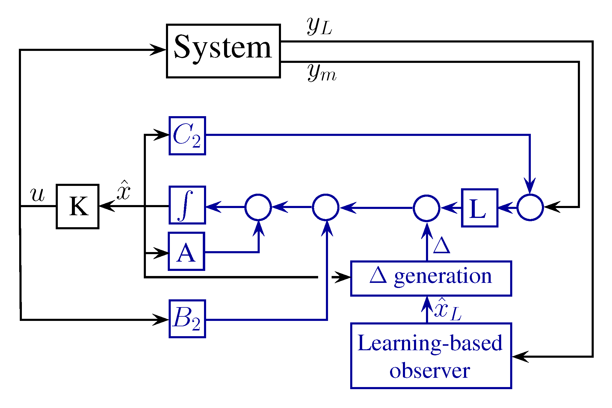
The result of the $\gamma$ minimization are the L and K matrices, with which the controlled system can be formulated. Figure 2 illustrates the implementation of the controlled systems with the observer. In the block Δ generation the rule (4) is implemented.

4. Application of the Observer Design to a Vehicle Control Problem

In the rest of the paper the proposed observer design framework for a vehicle control problem is applied. The goal of the observer is to provide a precise lateral velocity value $v_y$ for the path tracking control, if the yaw-rate $\dot{\psi }$ and the lateral error of the vehicle from the path $e_y=y-y_{ref}$ are measured.

The model-based representation of the system is based on the two-wheel bicycle model of a medium-size passenger car [16], such as

$$\begin{array}{cc}\hfill J\ddot{\psi }& =C_f{l}_1\left(\delta -\frac{v_y+\dot{\psi }{l}_1}{v}\right)-C_r{l}_2\left(-\frac{v_y-\dot{\psi }{l}_2}{v}\right),\hfill \end{array}$$

(12a)

$$\begin{array}{cc}\hfill m{\dot{v}}_y& =C_f\left(\delta -\frac{v_y+\dot{\psi }{l}_1}{v}\right)+C_r\left(-\frac{v_y-\dot{\psi }{l}_2}{v}\right),\hfill \end{array}$$

(12b)

$$\begin{array}{cc}\hfill \dot{y}& =v_y,\hfill \end{array}$$

(12c)

and the model-based formulation is

$$\begin{array}{c}\hfill \dot{x}=Ax+B_{2}u,\end{array}$$

(13)

where the state vector is $x^T=[\dot{\psi },v_y,y]$ and $C_r=$ 126,000 N/rad, $C_f=$ 126,000 N/rad are the cornering stiffness values on the front and rear wheels, $l_f=1.47$ m, $l_r=1.5$ m are the distances between the front/rear axles and the center of gravity. The mass of the vehicle is $m=2108$ kg and the inertia value on the vertical axis is $J=$ 1585.3 kg m${}^2$. In the design of the observer and the controller $v=20$ m/s constant longitudinal velocity is considered.

The performance of the controller is formed as

$$\begin{array}{c}\hfill z_c=e_y=y-y_{ref}=C_{1,c}x+y_{ref},\end{array}$$

(14)

where $y_{ref}$ is the reference position of the vehicle. Since $y_{ref}$ reference signal can be handled as a disturbance in the system, which offsets the value of y for the controller, it is not considered directly in the design of K.

The computation of the control input u requires the states of the system because of the full-state feedback. Since $\dot{\psi }$ and y are considered to be measured, an accurate observation on the state ${\widehat{v}}_y$ must be provided. Therefore, the performance criteria of the observer design is to minimize ${({\widehat{v}}_y-v_y)}^2$. In the implementation of the controller and the observer the coordinate system of the vehicle is handled to move together with the vehicle. It results in that the lateral position of the vehicle in the implementation of the controller is equal to the measured lateral error $e_y$. Thus, for implementation purposes, the vector of the measured signal is $y_m^T=[\dot{\psi },e_y]$.

The ${\mathsf{\Delta }}_{min,i},{\mathsf{\Delta }}_{max,i}$ values for the generation of $\mathsf{\Delta }$ signal are selected with the same absolute values, such as $|{\mathsf{\Delta }}_{min,i}|=|{\mathsf{\Delta }}_{max,i}|$, $\forall i\in n$. The value for $v_y$ is $\pm 0.15$ m/s, for $\dot{\psi }$ it is $\pm 0.1$ rad/s and for $e_y$ it is $\pm 0.2$ m. Moreover, the design of the model-based observer requires the selection of $Q_o$ and $r_o$. In the given observer design problem the $Q_o$ is suggested to select in the form of a matrix, whose elements outside of the main diagonal are zero. The values in the main diagonal represent the priority of $v_y$ observation, i.e., the related value of $Q_o$ to $v_y$ is suggested to selected as a high value. Nevertheless, the selection of $Q_o,r_o$ is a tuning process, until the requested performance level of the observer is reached.

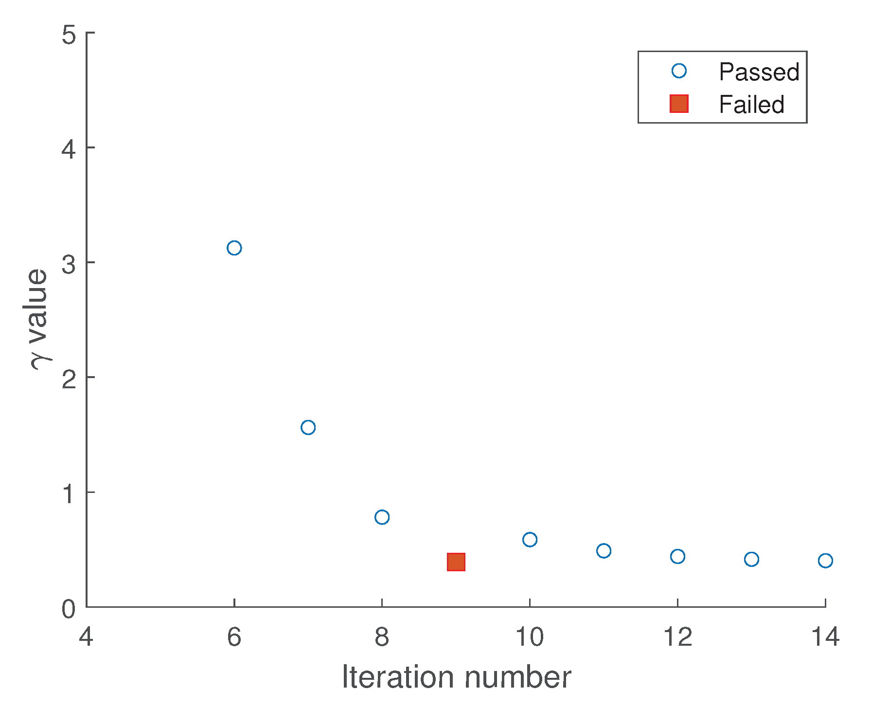
The result of the $\gamma$ minimization is illustrated in Figure 3. The initial value of the candidate $\gamma$ value is 100 and the achieved minimum value is $0.4028$, see step 14. During the minimization process in step 9 with the candidate $\gamma$ value $0.3906$ the minimization is failed, i.e., $X,Y$ matrices cannot be existed. Since the value in step 14 is close to the value in step 9, it can be selected as a minimum for $\gamma$. The achieved $\gamma$ value guarantees the robustness of the system due to $\gamma <1$.

4.1. Training of the Learning-Based Observer

In the vehicle control example a neural network-based observer is implemented in order to increase the accuracy of the estimation process. The goal of the learning-based observer is to provide an estimation on ${\widehat{x}}_L$, which is carried out through the following signals, which can be measured by the on-board sensors of the vehicle:

• longitudinal velocity v,
• lateral acceleration ${\dot{v}}_y$,
• steering angle $\delta$,
• yaw-rate $\dot{\psi }$.

The training process of the neural network is performed using supervised learning, for which a previously recorded training dataset is used. During the data generation several simulations are performed in CarMaker vehicle dynamics simulation software. The steering angle of the vehicle was randomized within the reasonable region.

Generally, neural networks are able to handle fitting problems, where the process is influenced by high nonlinearities. Neural networks consist of several layers, which can be divided into three main groups such as the input layer hidden layers and the output layer. The layers consist of neurons, which is built up by activation functions and weights. Before the training process, several parameters are be chosen such as the number of the layers and neurons, which are determined using the k-fold cross-validation technique [17]. Moreover, taking into account the chosen activation functions, the number of neurons can be determined see [18].

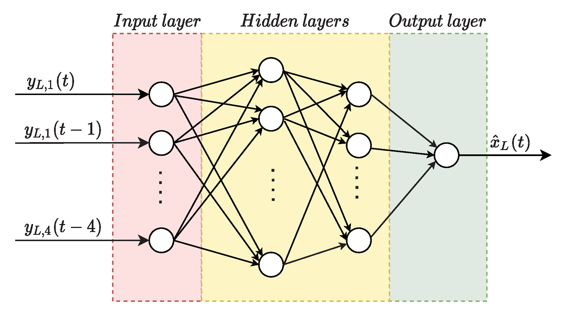
In Figure 4 the structure of the selected neural network is illustrated, in which the inputs of the network is given by $(y_{l,i})$ and the output is ${\widehat{x}}_l$.

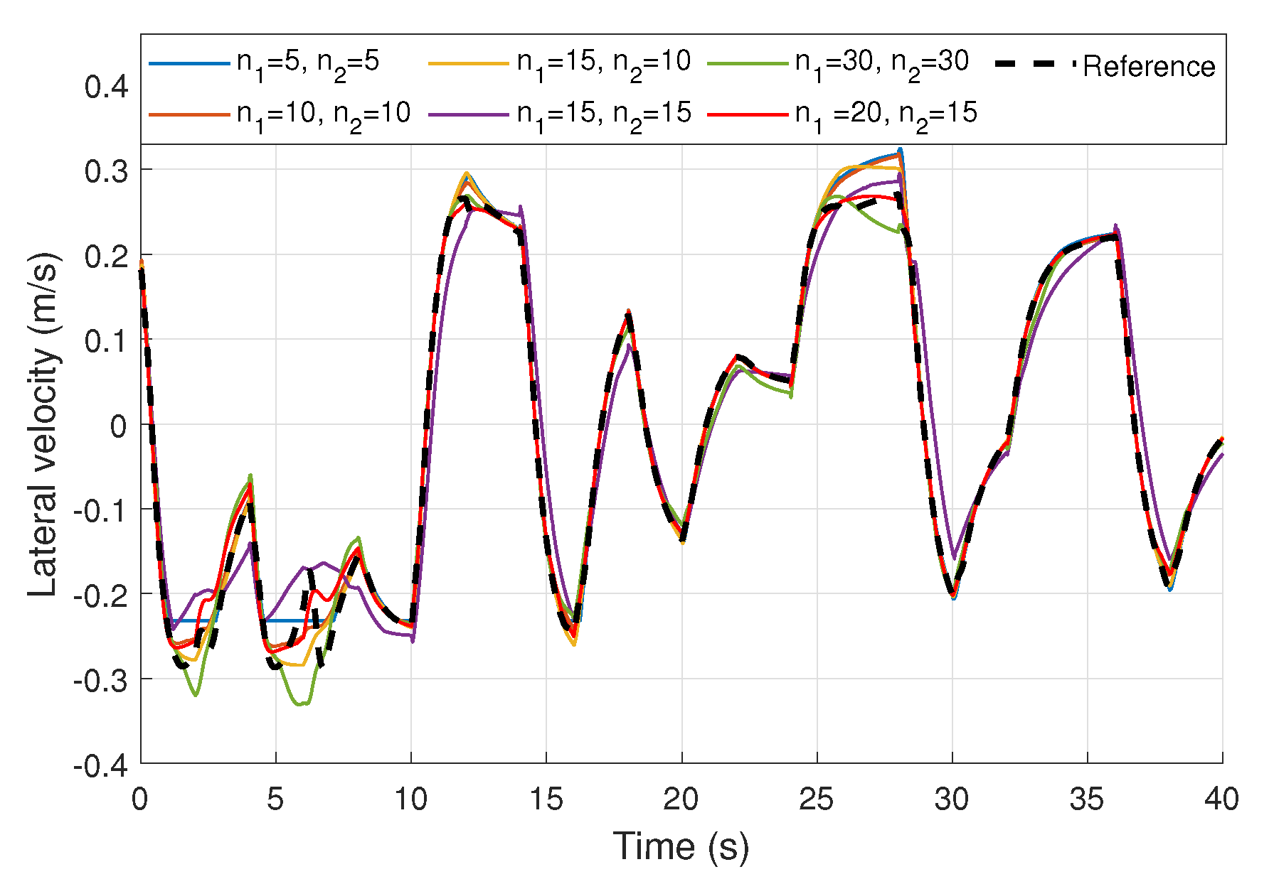
Since the accuracy of the estimation process can be increased by considering past values, the neural network-based observer takes into account the actual and 3 past values of the measured attributes. The sampling time of the past values can be determined using spectral analysis [19]. In Figure 5 an example can be seen for the results of the estimation process with various numbers of neurons in the hidden layers ($n_1$-first hidden layer, $n_2$-second hidden layer). It can be said that by increasing the number of neurons, a better estimation accuracy can be achieved. However, using too many neurons leads to over-fitting, which greatly decrease the usability of the network. As a result,

Table 1. Parameters of the trained neural network.

Parameters of the Neural Network
	1st Hidden Layer	2nd Hidden Layer
Number of neurons	20	15
Activation function	ReLU	log-sigmoid

summarizes the main parameters of the neural network with the lowest sum of error value, i.e., the selected number of neurons and the types of activation function.

The training process is performed using a backpropagation algorithm, and parameters of the neural network is calculated using Levenberg-Marquardt optimization process.

4.2. Simulation Results

Finally, the effectiveness of the proposed observer design framework is presented through a comprehensive simulation example. The simulations are performed in CarMaker vehicle dynamic simulation software, in which the vehicle is driven along a predefined path. Two different cases are compared during the simulations. In the first case, the measured signals of the sensors on the vehicle are considered to be accurate. But, in the second case, additional noise with high value is added to the measured signals in order to simulate the case, when the learning-based observer can provide inaccurate ${\widehat{x}}_L$. The goal of the simulations is to show that through learning-based observer the state observation process can be improved and furthermore, the proposed design framework provides guarantees if the output of learning-based observer is degraded.

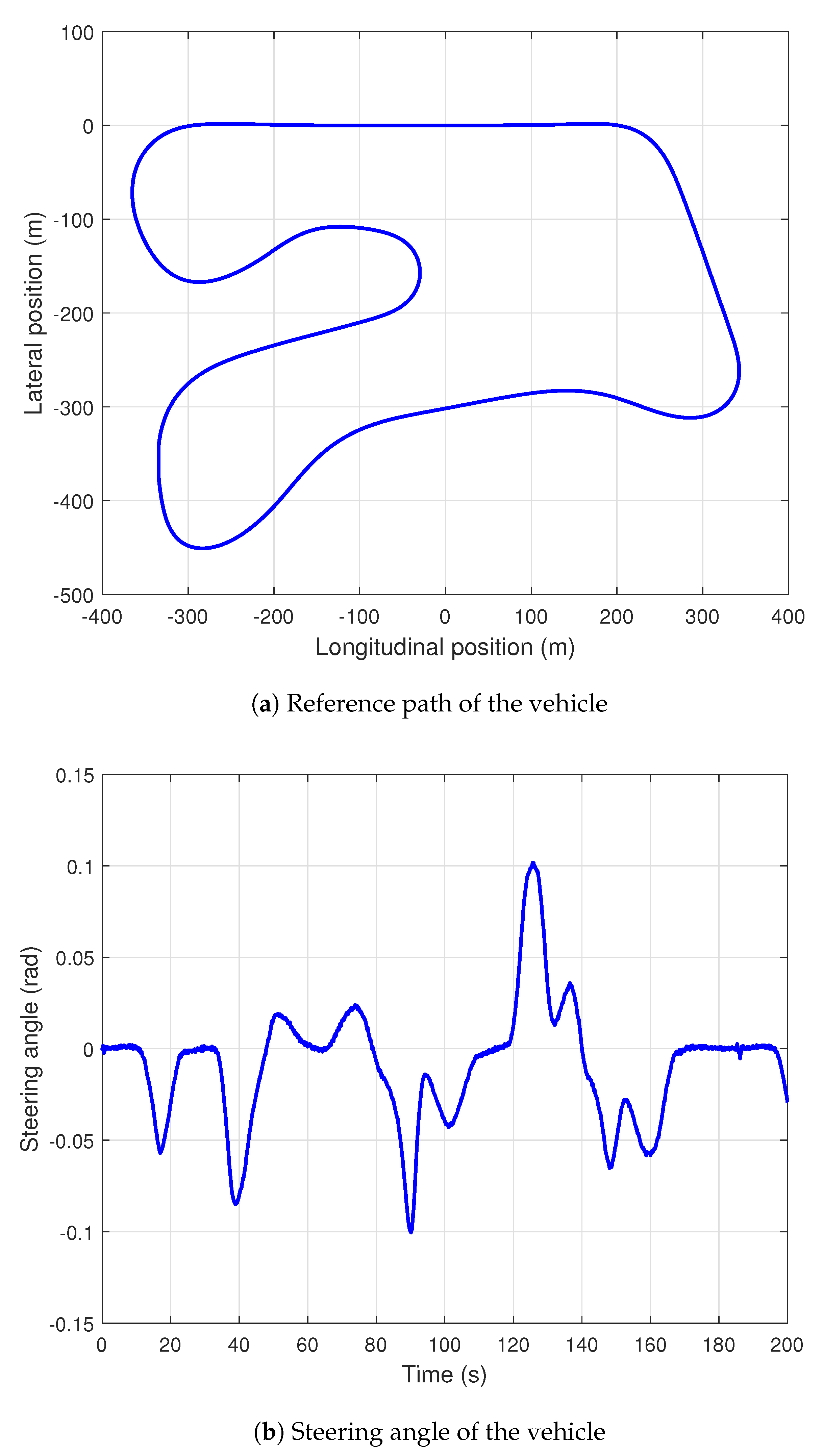
In Figure 6a the reference trajectory of the vehicle can be seen, which is based on the data of a section of Hockenheimring, Germany. The steering angle, which is provided by the resulted controller K, is shown in Figure 6b. During the simulation example, the longitudinal velocity of the controlled vehicle is set to 50 km/h.

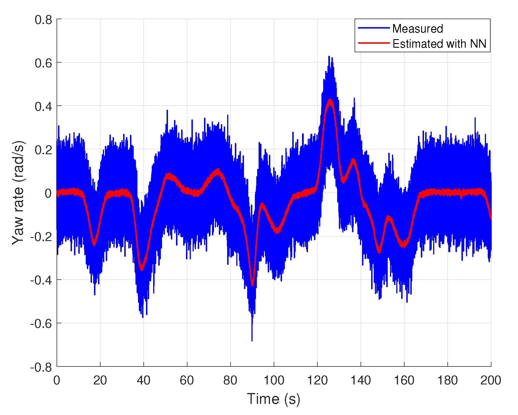
In Figure 7 the yaw-rate of the vehicle is depicted. The figure shows that the measured yaw-rate signal is quite noisy. Using the proposed observer, which is augmented with the results of the neural network, the obtained yaw-rate value can be used during the lateral control of the vehicle. Thus, the impact of the noise on the control performance can be reduced though the proposed method.

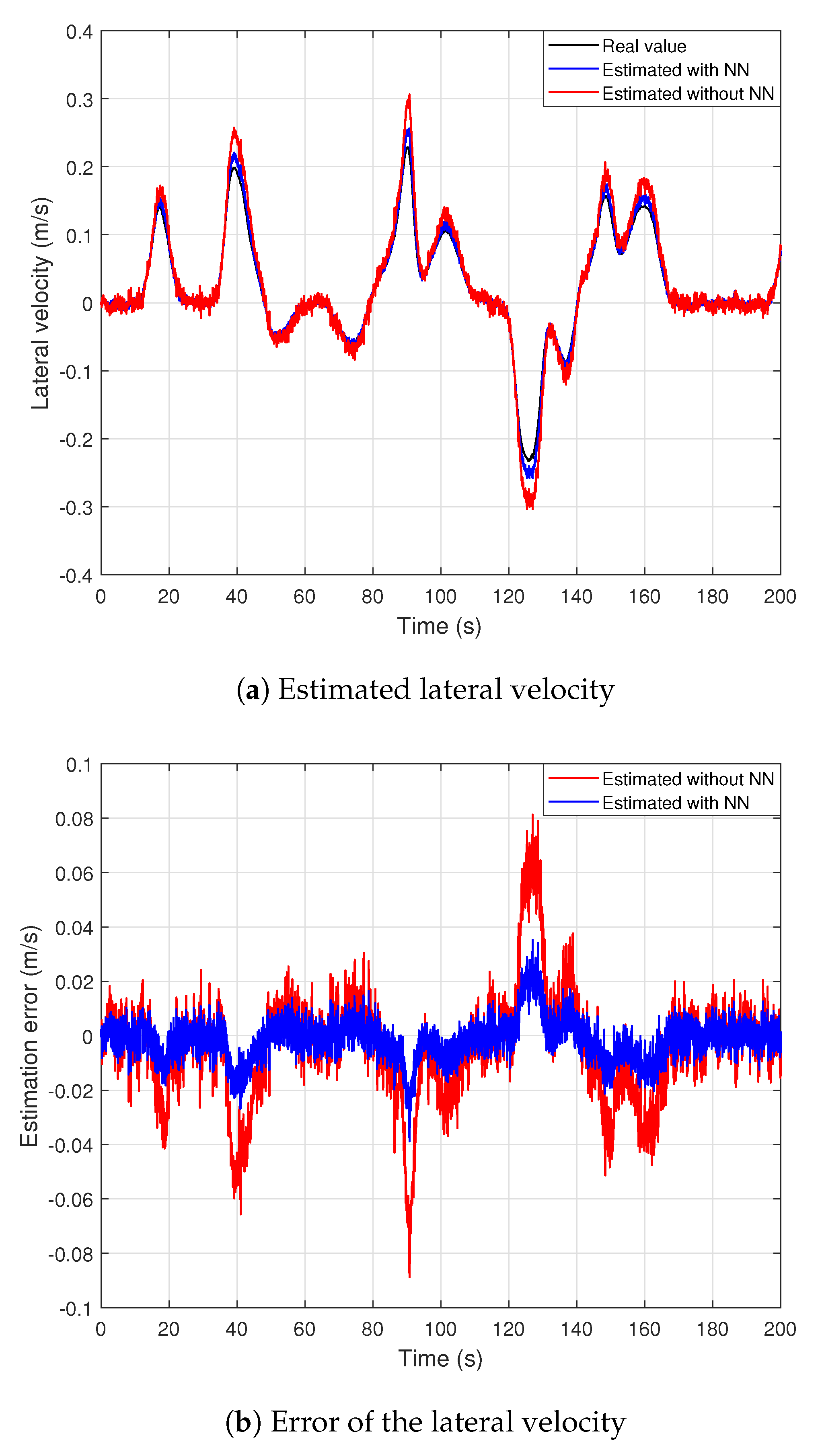
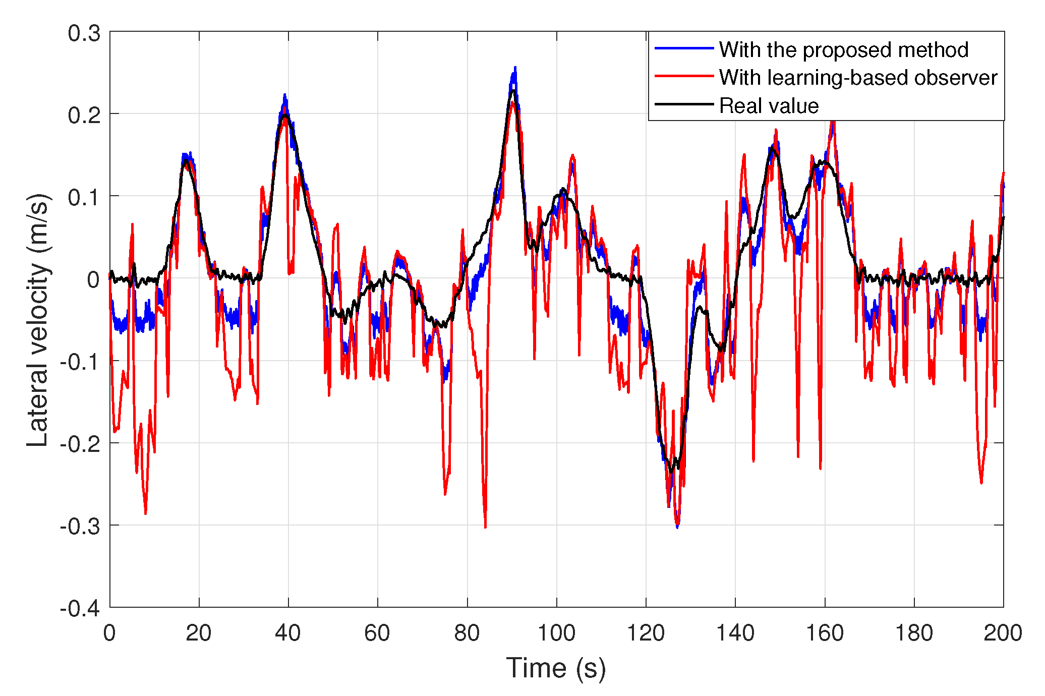
In Figure 8a the estimated lateral velocities can be seen. The real value of the lateral velocity is represented with the black line and the red line illustrates the results of the model-based observer. Moreover, the lateral velocities provided by the observer, which is extended with the neural network, is shown with the blue line. It can be seen, that using the proposed observer structure, the results of the estimation process is more accurate compared to the purely model-based solution. Furthermore, it can be said that the choice of ${\mathsf{\Delta }}_{min},{\mathsf{\Delta }}_{max}$ has high impact on the results. In the cases when the neural network provides more accurate results than the model-based observer, the estimation accuracy can be highly increased. But, when the neural network provides poor results, avoiding inaccuracy of the state observation process can be guaranteed by the robust ${\mathcal{H}}_{\infty }$ design of the model-based observer.

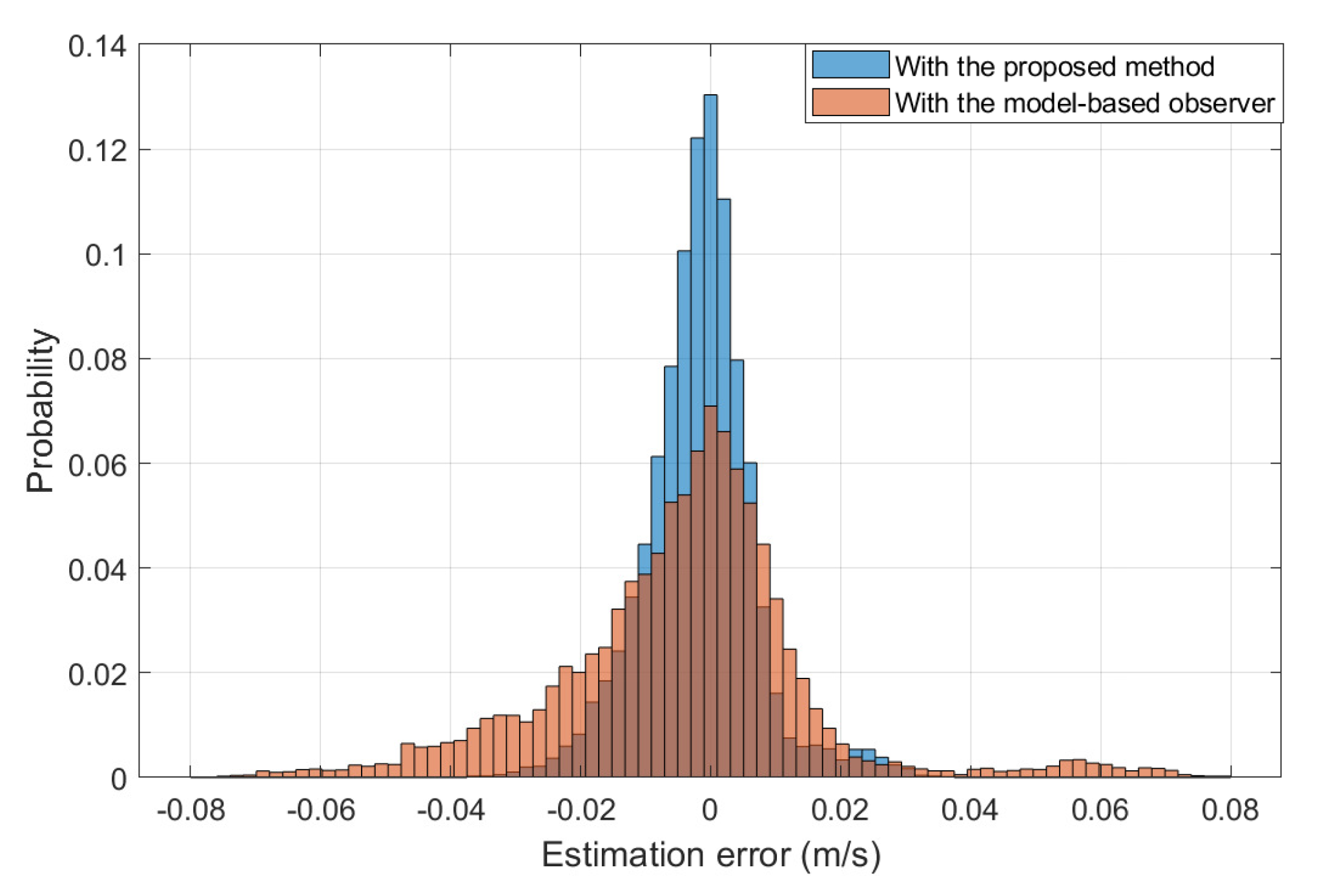
In Figure 9 a statistical analysis, i.e., a histogram is presented for the illustration of the effectiveness of the observer. In the histogram the probability values of each estimation errors on $v_y$ are illustrated. The blue bars represent the results with the proposed method, in which the outputs of the neural network are taken in to account. The statistical analysis confirms the conclusions of the simulation results.

In the second example noises with high values on the measurements are added, which leads to the inaccurate operation of the learning-based observer. The result of the observation on $v_y$ is shown in Figure 10. It can be seen that in this case the error between ${\widehat{x}}_L$ and x is significantly increased and thus, $\widehat{x}\ne {\widehat{x}}_L$ in most of the simulation. Nevertheless, the degradation of the observation process is limited, due to the limitation of $\mathsf{\Delta }$.

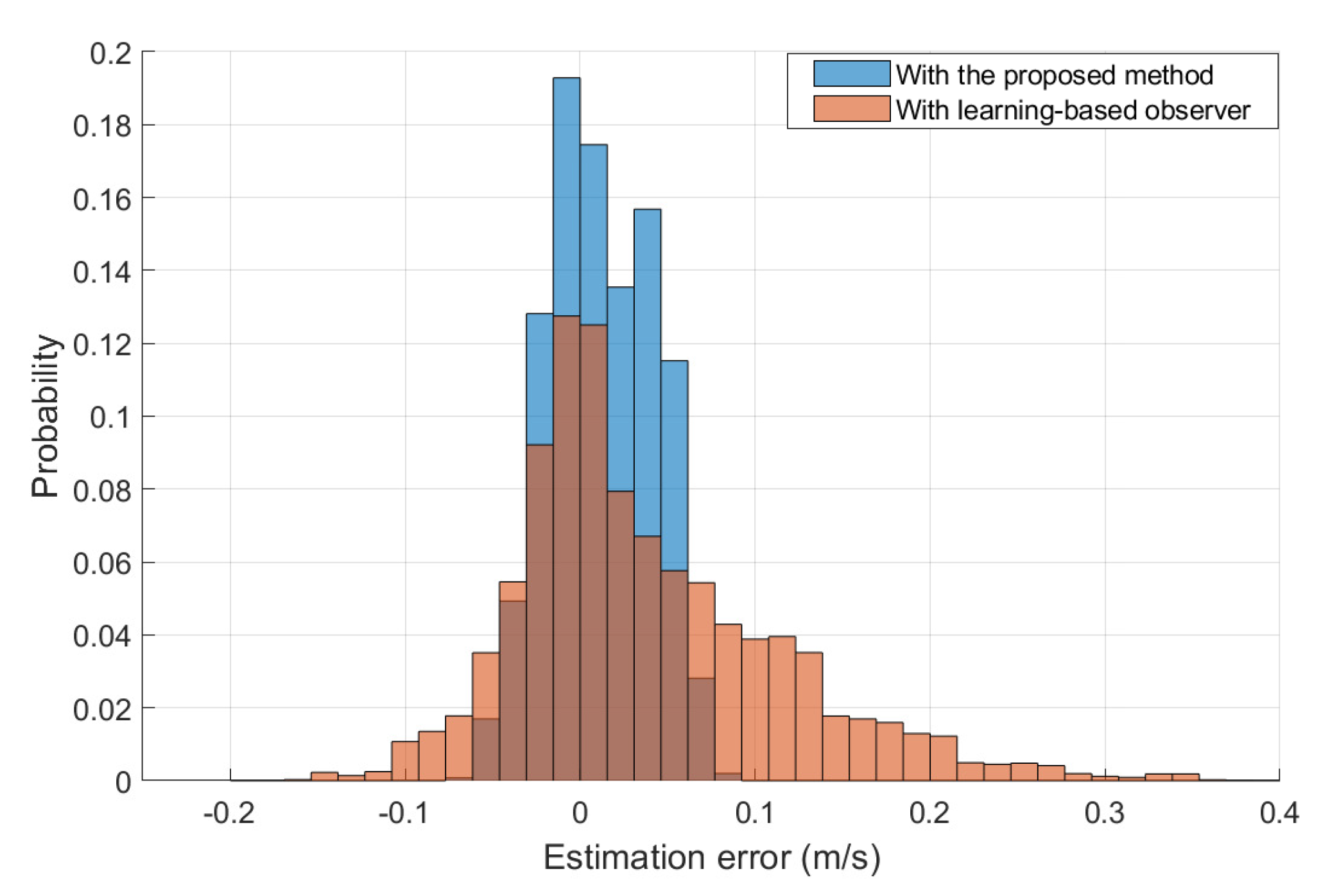
The statistical analysis through the plot of the histogram on the results of the second simulation is found in Figure 11. It shows the main benefit of the method, i.e., the guarantee on the estimation error. In case of the proposed method the plot of the histogram is bounded, while without the limitation of $\mathsf{\Delta }$ the neural-network-based observer leads to a flatter plot without limits on the error.

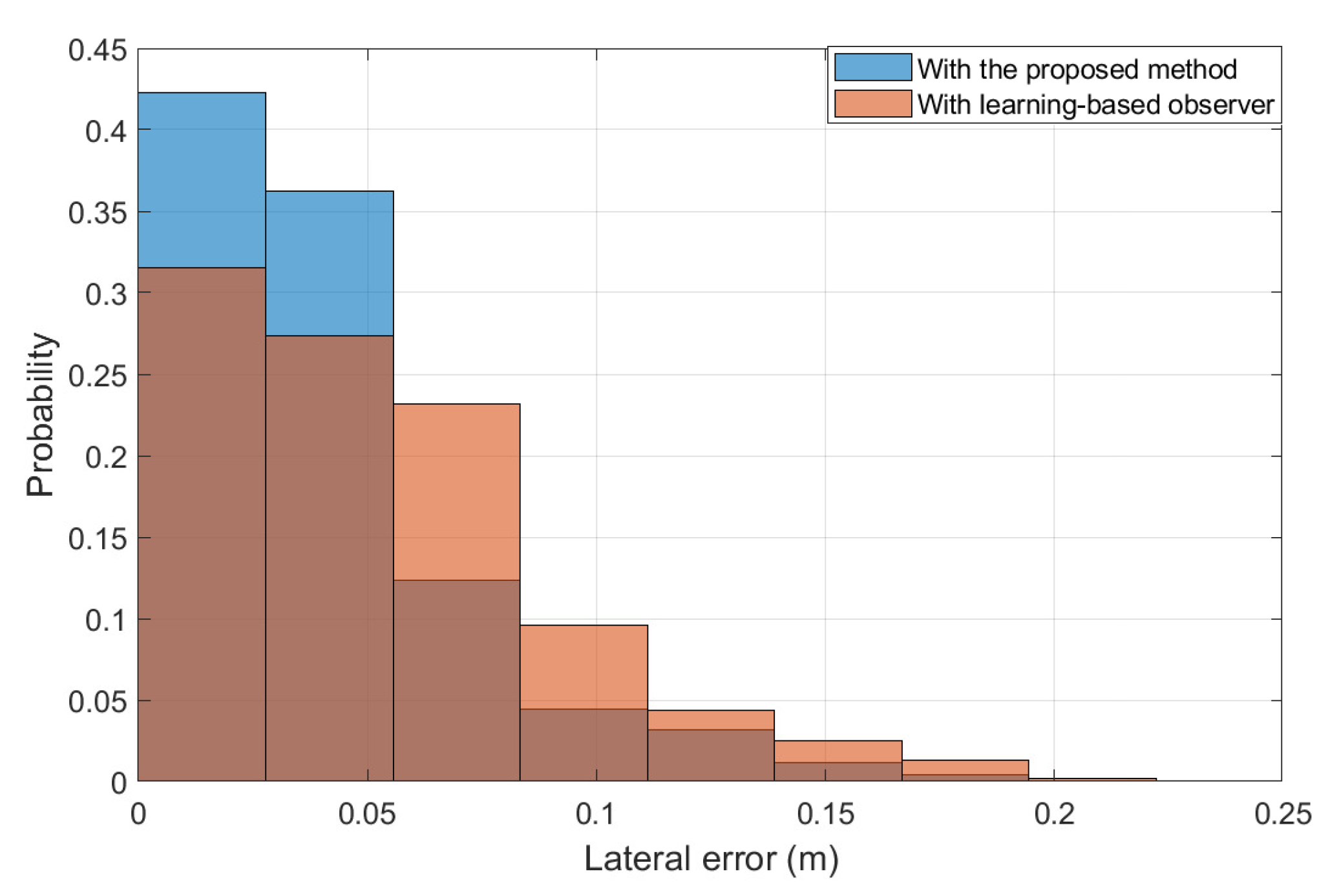
Since in the proposed example the observed state $\widehat{x}$ is used for control purposes, the impact of the observation accuracy on the tracking performance is examined. Figure 12 shows the histogram on the absolute value of the lateral tracking error in case of the second scenario. It can be seen that the proposed method results in reduced lateral error with increased probability, compared to the simulation with learning-based observer. The improvement is around ≈25% if $|e_y|<0.05$ m.

5. Conclusions

The simulation examples proposed the effectiveness of the method on a vehicle control problem from two aspects. First, through the design framework the higher accuracy of the learning-based observer can be utilized in the state observation process. Second, if the learning-based observation has degradation, the degradation of the state observation process can be limited. The advantageous operation of the designed observer is achieved through the robust ${\mathcal{H}}_{\infty }$ observer design method. The effectiveness of the design method has been illustrated through simulations on the example of state estimation for lateral dynamics of vehicles. The statistical evaluation of the results has concluded that the estimation error through the proposed method can be limited and similarly, the performance level of the observation process is improved. Finally, the observer design method is extended with the design method of the controller, which leads to a joint ${\mathcal{H}}_{\infty }$ design.

Nevertheless, the proposed method has some limitations, which must be handled through the practical application of the method. First, the training of the learning-based observer requires high number of data, which can be achieved through simulations or test measurements. In some applications the collection of high number of data can be expensive and the unsuccessful scenarios during the training process can lead to critical operation. Therefore, a challenge of the learning-based observation is to provide a method, with which a quantity index of the required number of samples can be given. A further limitation of the method is that it uses linear model for the design of the model-based observer. A future goal is to extend the design process for further class of systems, e.g., linear parameter varying systems. Another future challenge of the method is to extend the state observation process for a prediction method of the states. It requests the development of a method on the comprehensive analysis of the learning-based agent, e.g., observer or predictor. In the proposed method the decision on the acceptability of the learning-based observation is based on the actual signals, but for prediction the output of the learning-based agent on a longer horizon must be examined, which is a challenge in the design framework. Furthermore, another challenge of the method is to guarantee the observability with the learning-based observer for a system, which is unobservable. It can require an analysis method on the global observability, which contains the augmented system, i.e., the system and the learning-based observer.

References

- Yin, Y.; Shi, P.; Liu, F.; Karimi, H.R. Continuous gain scheduled h-infinity observer for uncertain nonlinear system with time-delay and actuator saturation. Am. Control Conf. (ACC) 2012, 8, 8077–8088. [Google Scholar]
- Wei, Z.; Leng, F.; He, Z.; Zhang, W.; Li, K. Online State of Charge and State of Health Estimation for a Lithium-Ion Battery Based on a Data-Model Fusion Method. Energies 2018, 11, 1810. [Google Scholar] [CrossRef] [Green Version]
- Aligia, D.A.; Roccia, B.A.; Angelo, C.H.D.; Magallan, G.A.; Gonzalez, G.N. An orientation estimation strategy for low cost IMU using a nonlinear Luenberger observer. Measurement 2021, 173, 108664. [Google Scholar] [CrossRef]
- Jung, J.; Huh, K.; Fathy, H.K.; Stein, J.L. Optimal robust adaptive observer design for a class of nonlinear systems via an H-infinity approach. Am. Control Conf. (ACC) 2006, 1627–1632. [Google Scholar] [CrossRef]
- Houimli, R.; Bedioui, N.; Besbes, M. An Improved Polytopic Adaptive LPV Observer Design Under Actuator Fault. Int. J. Control. Autom. Syst. 2018, 16, 168–180. [Google Scholar] [CrossRef]
- Do, M.H.; Koenig, D.; Theilliol, D. Robust observer-based controller for uncertain-stochastic linear parameter-varying (LPV) system under actuator degradation. Int. J. Robust Nonlinear Control 2018, 31, 168–180. [Google Scholar]
- Theocharis, J.; Petridis, V. Neural network observer for induction motor control. IEEE Control Syst. Mag. 1994, 14, 26–37. [Google Scholar]
- Zhang, C.; Sun, T.; Pan, Y. Neural Network Observer-Based Finite-Time Formation Control of Mobile Robots. Math. Probl. Eng. 2014, 2014. [Google Scholar] [CrossRef] [Green Version]
- Alhajeri, M.S.; Wua, Z.; Rincona, D.; Albalawi, F.; Christofides, P.D. Machine-learning-based state estimation and predictive control of nonlinear processes. Chem. Eng. Res. Des. 2021, 167, 268–280. [Google Scholar] [CrossRef]
- Cao, X.; Bi, M. Extended Luenberger Observer Based on Dynamic Neural Network for Inertia Identification in PMSM Servo System. In Proceedings of the Fifth International Conference on Natural Computation, Tianjian, China, 14–16 August 2009. [Google Scholar]
- Boada, B.L.; Boada, M.J.L.; Vargas-Melendez, L.; Diaz, V. A robust observer based on H infinity filtering with parameter uncertainties combined with Neural Networks for estimation of vehicle roll angle. Mech. Syst. Signal Process. 2018, 99, 611–623. [Google Scholar] [CrossRef] [Green Version]
- Schinkel, W.; van der Sande, T.; Nijmeijer, H. State Estimation for Cooperative Lateral Vehicle Following Using Vehicle-to-Vehicle Communication. Electronics 2021, 10, 651. [Google Scholar] [CrossRef]
- Li, Y.; Xiong, B.; Vilathgamuwa, D.M.; Wei, Z.; Xie, C.; Zou, C. Constrained Ensemble Kalman Filter for Distributed Electrochemical State Estimation of Lithium-Ion Batteries. IEEE Trans. Ind. Inf. 2021, 17, 240–250. [Google Scholar] [CrossRef]
- Wei, Z.; Zhao, J.; Ji, D.; Tseng, K.J. A multi-timescale estimator for battery state of charge and capacity dual estimation based on an online identified model. Appl. Energy 2017, 204, 1264–1274. [Google Scholar] [CrossRef]
- Gahinet, P.; Apkarian, P. A linear matrix inequality approach to Hinf control. Int. J. Robust Nonlinear Control 1994, 4, 421–448. [Google Scholar] [CrossRef]
- Rajamani, R. Vehicle Dynamics and Control; Springer: Berlin, Germany, 2005. [Google Scholar]
- Demut, H.; Hagan, M.; Beale, M. Neural Network Design; PWS Publishing Co.: New York, NY, USA, 1997. [Google Scholar]
- Xu, S.; Chen, L. A novel approach for determining the optimal number of hidden layer neurons for FNN’s and its application in data mining. In Proceedings of the 5th International Conference on Information Technology and Applications (ICITA 2008), Cairns, Australia, 23–26 June 2008; pp. 683–686. [Google Scholar]
- Hegedus, T.; Fenyes, D.; Nemeth, B.; Gaspar, P. Handling of tire pressure variation in autonomous vehicles: An integrated estimation and control design approach. In Proceedings of the 2020 American Control Conference, Denver, CO, USA, 1–3 July 2020; pp. 2244–2249. [Google Scholar]
Figure 1.
Illustration of the framework for observer design.
Figure 2.
Scheme of the implementation of the observer and the controller.
Figure 3.
Convergence of the minimization.
Figure 4.
Structure of the neural network.
Figure 5.
Results of neural networks with different parameters.
Figure 6.
Control input and the reference trajectory during the simulation example.
Figure 7.
Yaw rate of the vehicle.
Figure 8.
Comparison of the model-based and neural-network-based results.
Figure 9.
Comparison between the model-based and the combined estimation.
Figure 10.
Estimated lateral velocity with false signals.
Figure 11.
Histogram on the observation error in the second scenario.
Figure 12.
Histogram on the lateral tracking error in the second scenario.