A Data-Driven Methodology for the Reliability Analysis of the Natural Gas Compressor Unit Considering Multiple Failure Modes

Abstract

In this study, a data-driven methodology for the reliability analysis of natural gas compressor units is developed, and both the historical failure data and performance data are employed. In this methodology, firstly, the reliability functions of the catastrophic failure and degradation failure are built. For catastrophic failure, the historical failure data are collected, and the rank regression model is utilized to obtain the reliability function of the catastrophic failure. For degradation failure, a support-vector machine is employed to predict the unit’s performance parameters, and the reliability function of the degradation failure is determined by comparing the performance parameters with the failure threshold. Finally, the reliability of the compressor unit is assessed and predicted by integrating the reliability functions of the catastrophic failure and the degradation failure, and both their correlation and competitiveness are considered. Furthermore, the developed methodology is applied to an actual compressor unit to confirm its feasibility, and the reliability of the compressor unit is predicted. The assessment results indicate the significant impact of the operating conditions on the precise forecasting of the performance parameters. Moreover, the effects of the value of the failure threshold and the correlation of the two failure modes on the reliability are investigated.

1. Introduction

Natural gas compressor units are widely used in natural gas pipeline networks [1,2,3,4]. For example, the natural gas in transmission pipeline systems is driven by compressor units to ensure continuous transport and delivery to its customers [5,6], and compressor units are also used in underground gas storage to increase the pressure of the natural gas to a level sufficient for injection [7,8]. Obviously, natural gas compressor units play a significant role in natural gas pipeline networks; thus, compressor unit failures are major threats to the security of the gas supply [9,10,11]. Therefore, the reliability of natural gas compressor units is an issue of high concern, and the aim of this study is to develop a systematic methodology to assess and predict the reliability of natural gas compressor units from a comprehensive perspective.

Considerable efforts have been devoted to developing qualitative and quantitative methods to assess the reliability of natural gas compressor units, mainly based on the analysis of failure data and structural reliability theory. In Ref. [12], the failure modes of the reciprocating compressor and the centrifugal compressor were studied, and the fault trees of these two types of compressors were constructed. In Ref. [13], failure modes and effects analysis (FMEA) was used to identify the weaknesses the compressors, and the finite element method was employed to calculate their reliability. In Ref. [11], the operation and shutdown data of 36 gas-turbine-driven compressor units in West–East Gas Pipelines I and II were collected to calculate the reliability indices of the compressor units. In Ref. [14], the limit state equations of the key components of the reciprocating compressors—including the crankshaft, connecting rod, piston rod, and cylinder—were established, and the structural reliability of each component was calculated based on the stress–strength interference model. In Refs. [15,16], the key reliability parameters of a refrigerator compressor in the design phase were identified via failure analysis, accelerated life testing, and corrective actions. The reliability of a scroll compressor was evaluated in Ref. [17], and its lifetime was estimated by using the data of zero-failure accelerated life testing.

The abovementioned approaches are mainly based on the analysis of the lifetime failure data of compressor units. In addition, performance data can also be used for the reliability evaluation of the units, which can be modeled using the degradation path model and stochastic processes [18,19]. For the degradation path model, Crk [20] used the multivariate multiple regression method to assess the reliability of the highly reliable components, subsystems, and whole systems. In Ref. [21], the performance data of the equipment was measured and forecasted by time-series analysis, and its real-time reliability was estimated by applying exponential smoothing with a linear level and trend adaptation. In Ref. [22], an exponential model was used to characterize the degradation process of the bearings, and the residual life distribution was thus obtained. Moreover, Bayesian updating methods were employed to update the stochastic parameters of the exponential degradation models. In Ref. [23], the historical fault data and monitoring data in operation were combined to establish a prediction model of the performance degradation trend, and the prediction model was then applied to maintain the optimization of the compressor-washing of a two-shaft gas turbine. Moreover, a gray model and the Markov model were used to describe the uncertainty in the performance degradation process in Ref. [24]. In order to predict the remaining useful life of gas turbine engines, linear and quadratic models were proposed to model the degradation model in Ref. [25], and compatibility checking was used to determine the transition point from a linear regression to a quadratic regression. In Refs. [26,27], a linear regression model was used to model the degradation process of gas turbine performance, and Monte Carlo simulation was then employed to predict its availability. In Ref. [28], the performance of a gas compressor was evaluated based on its isentropic head, and the performance degradation of the gas compressors was further predicted using genetic programming.

In addition to degradation path models, stochastic processes are widely used in the analysis of performance data, and the Wiener process, gamma process, and inverse Gaussian process are also widely used. To be specific, a new class of Wiener process models was developed to model a system with a high degradation rate in Ref. [29]. In Ref. [30], the age-dependent Wiener process and the age-dependent gamma process were adopted to describe the degradation process. In Ref. [31], inverse Gaussian process models were proposed to analyze the degradation process, and Bayesian analysis was used in the modeling and inference.

It should be pointed out that there are some deficiencies in the current research on the reliability of compressor units using failure or performance data and structural reliability methods. First, natural gas compressor units have extremely high reliability, and for a specific compressor unit, the historical failure and maintenance data are much less numerous than the performance data. Therefore, it is difficult to collect the historical failure data for a specific compressor unit. Second, the structural reliability methods are very suitable for the reliability analysis of components of the compressor unit, but these methods are of limited usefulness from the overall and comprehensive perspectives. Finally, natural gas compressor units are typical complex mechanical power systems, which usually have two distinctive failure modes, i.e., degradation failure and catastrophic failure, and each failure mode is usually competing and correlated [32]. Therefore, only considering the degradation failure process will lead to inaccurate inferences of the compressor unit’s reliability. Furthermore, neither the classical degradation path model nor the stochastic process approach are effective enough to consider the impact of the external environment and operating conditions on the reliability of the compressor unit.

Therefore, in order to overcome these deficiencies, a data-driven methodology of reliability analysis, utilizing the historical failure data and the performance data of the natural gas compressor unit, is developed in this study, and is intended to provide reliability evaluation and prediction results from a comprehensive perspective. In this methodology, the two distinctive failure modes—i.e., degradation failure and catastrophic failure—and the effects of the external environment and operating conditions on the reliability of the compressor unit are all taken into consideration. The innovative contributions of this work are listed in detail as follows:

(1)

A data-driven method for reliability analysis of the compressor unit is developed.

(2)

The competitiveness and correlation of the two failure modes are considered.

(3)

The effects of the external environment and operating conditions are investigated.

(4)

The reliability of the compressor unit is predicted from a comprehensive perspective.

Aiming at developing this data-driven methodology, two types of failure modes—namely, catastrophic failure and degradation failure—are studied. According to the characteristics of the data and failure mode, the initial reliability functions of the catastrophic failure and degradation failure are built, respectively. For catastrophic failure, the historical failure data of both the unit in question and others of the same type caused by the catastrophic failure mode are collected. The rank regression model is then used to obtain the reliability function of the catastrophic failure. In terms of degradation failure, multivariate time-series analysis via a support-vector machine (SVM) is then adopted to forecast the performance parameters over a future time period, based on recent performance information and the specific load task. Moreover, the reliability function associated with the degradation failure is calculated by comparing the performance parameters with a pre-specified threshold. Finally, the reliability of the natural gas compressor unit is assessed and predicted by integrating the reliability functions of the catastrophic failure and degradation failure, and both the correlation and the competitiveness of the two failure modes are taken into account in the process.

2. The Data-Driven Methodology

The performance of most physical assets degrades over time, and follows certain failure patterns. Research results reveal that there are at least 6 failure patterns that occur in practice. Natural gas compressor units are typical complex mechanical power systems, and their fault modes can result in two different types of consequences, i.e., leading equipment to stop working suddenly, or performance degradation of equipment. In more detail, the natural gas compressor unit may suddenly fail due to hidden manufacturing defects, excessive loads, shocks, or other stresses, which is known as hard failure, or catastrophic failure. Moreover, the performance of the natural gas compressor unit may also gradually deteriorate due to wear, fatigue, erosion, and other causes, which is usually referred to as soft failure, or degradation failure. The catastrophic failure and degradation failure are correlated and competing. Therefore, in order to develop a data-driven methodology for the reliability analysis of natural gas compressor units, the reliability functions of the catastrophic and degradation failure must first be built. The historical failure data and the performance data of the natural gas compressor unit are then both collected and employed. Afterwards, by integrating the reliability functions of the catastrophic failure and degradation failure, and considering the correlation and competitiveness between the two failure modes simultaneously, the reliability of the compressor unit is evaluated and predicted from a comprehensive perspective.

Catastrophic failure is also called hard failure, in which a unit suddenly fails as a result of some external shock(s), such as power supply failure due to lightning, communication faults, etc. Therefore, a catastrophic failure is generally represented by two states—a normal operating state (denoted as 1), and a failed state (denoted as 0)—as shown in Figure 1 [33]. In contrast, degradation failure is also called soft failure, in which a failure occurs when the unit’s performance deteriorates to a pre-specified threshold due to wear, fatigue, erosion, or other causes [34], as also shown in Figure 1. Unlike catastrophic failure, when the degradation failure occurs, the unit is still working, albeit at a reduced level of performance. Note that the nomenclature of the variables in Figure 1 is listed in the Nomenclature section.

Consequently, in the event of two competing failure modes, the failure of the compressor unit depends on which of the two failures occurs first. Therefore, the reliability of the natural gas compressor unit R(t) for a period of time t can be denoted as follows:

$$R(t)=\mathrm{P}\mathrm{rob}\left[T>t\right]=\mathrm{P}\mathrm{rob}\left[\min \left\{T_c,T_d\right\}>t\right]$$

(1)

where t denotes the mission time of the compressor unit, T is the time to failure, and more specifically, T_c is the time to catastrophic failure, T_d is the time to degradation failure, and $\mathrm{Prob}\left[A\right]$ represents the probability of the event A. A block diagram of the stages of reliability analysis of the natural gas compressor is shown in Figure 2.

Moreover, because the catastrophic failure and the degradation failure are influenced by one another, the failures of the individual modes are likely to be correlated events in the real world [35]. Therefore, for a compressor unit with two correlated failure modes, the reliability function R(t) or failure probability function P_f(t) can be expressed as follows:

$$\begin{array}{l}{P}_f(t)=\mathrm{Prob}\left[E_1\cup E_2\right]\\ =\mathrm{Prob}\left[E_1\right]+\mathrm{Prob}\left[E_2\right]-\mathrm{Prob}\left[E_1\cap E_2\right]\\ =P_c(t)+P_d(t)-\mathrm{Prob}\left[E_1\cap E_2\right]\end{array}$$

(2)

where E₁ and E₂ denote the catastrophic failure event and the degradation failure event during the mission time, respectively, and $P_f(t)=1-R(t)$, $P_c(t)=1-R_c(t)$, $P_d(t)=1-R_d(t)$; R_c(t) and R_d(t) are the reliability functions for the catastrophic failure and degradation failure, respectively, and P_c(t) and P_d(t) are their corresponding failure probabilities; $\cup$ and $\cap$ denote the intersection and union, respectively, while $\mathrm{Prob}\left[E_1\cap E_2\right]$ is the joint probability of the simultaneous occurrence of both catastrophic and degradation failure events during the mission time.

As shown in Equation (2), we know that the calculation of the reliability for the catastrophic failure and the degradation failure, along with solving $\mathrm{Prob}\left[E_1\cap E_2\right]$, are the major challenges in the data-driven methodology. The steps to obtain the reliability functions of the catastrophic failure and degradation failure are illustrated in Section 2.1 and Section 2.2, respectively. The procedure to solve the joint probability $\mathrm{Prob}\left[E_1\cap E_2\right]$ is shown in Section 2.3.

2.1. Reliability Function of the Catastrophic Failure

For the catastrophic failure mode, the historical failure data of the compressor unit and other units of the same type caused by catastrophic failure are all collected. The rank regression model [36,37] is then used to calculate the reliability function R_c(t) or the failure probability function P_c(t). The steps of the rank regression model are given as follows:

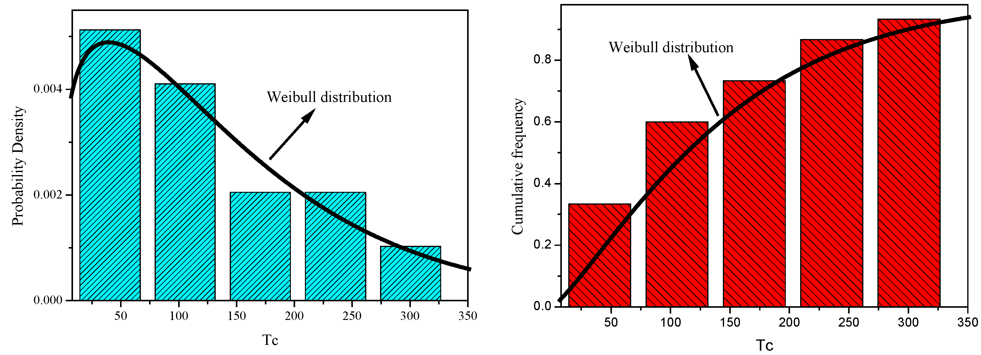
Step 1: The frequency histogram and cumulative frequency histogram of the time to catastrophic failure T_c are plotted, and the cumulative frequencies $F(t_i),i=1,\dots k$ are then obtained, where k is the number of groups of the frequency histogram, and is determined by the empirical formula $k=1+3.3\lg n$, while n is the failure time, and t_i is the center value of each group.

Step 2: Exponential distribution, normal distribution, Log-normal distribution, Weibull distribution, and Gumbel distribution are selected as the candidate distributions. Thereafter, the cumulative distribution function (CDF) and the linear form for each distribution are listed in

Table 1. The CDF and linear form for each distribution.

Distribution	CDF	$\mathbf{Linear} \mathbf{Form} (\mathit{y}=\mathit{A}+\mathit{B}x)$
Exponential distribution	$F(t)=1-\exp (-\lambda t)$	$\begin{array}{l}y=\ln (1-F(t)),x=t\\ A=0,B=-\lambda \end{array}$
Normal distribution	$F(t)=\Phi (\frac{t-\mu }{\sigma })$	$\begin{array}{l}y={\Phi }^{-1}(t),x=t\\ A=-\frac{\mu }{\sigma };B=\frac{1}{\sigma }\end{array}$
Log-normal distribution	$F(t)=\Phi (\frac{\ln t-\mu }{\sigma })$	$\begin{array}{l}y={\Phi }^{-1}(t),x=\ln t\\ A=-\frac{\mu }{\sigma },B=\frac{1}{\sigma }\end{array}$
Weibull distribution	$F(t)=1-\exp \left[-{\left(\frac{t}{\mu }\right)}^{\sigma }\right]$	$\begin{array}{l}y=\ln (-\ln (1-F(t))),x=\ln t\\ A=-\sigma \ln \mu ,B=\sigma \end{array}$
Gumbel distribution	$F(t)=\exp (-\exp (-\frac{t-\mu }{\sigma }))$	$\begin{array}{l}y=\ln (-\ln (F(t))),x=t\\ A=\frac{\mu }{\sigma },B=-\frac{1}{\sigma }\end{array}$

where $\Phi$ is the standard normal cumulative distribution function, and ${\Phi }^{-1}$ is the inverse function of the standard normal cumulative distribution function.

.

Step 3: The cumulative frequencies $F(t_i),i=1,\dots k$ obtained in Step 1 are fitted by the least squares method according to the five linear forms shown in Table 1, and the correlation coefficient ρ of each fitting is also calculated.

Step 4: Based on the calculation results of the correlation coefficient in Step 3, the optimal distribution for the time to catastrophic failures T_c is selected, namely, the failure probability function P_c(t). Moreover, Pearson’s chi-squared test is used to determine whether the time to catastrophic failure matches the selected optimal distribution.

2.2. Reliability Function for Degradation Failure

In the degradation failure mode, the failures of the compressor units are defined in terms of the physical performance parameters decreasing to below a given critical threshold [38,39]. For example, in Ref. [23], the efficiency of the compressor was adopted as the performance parameter to describe the health of the compressor, and the critical degradation threshold was taken as 2.8% compressor efficiency degradation. Let $Y(t_i)$ denote the actual value of the performance parameter with respect to time t_i, which can be directly calculated from the unit’s historical operating data at the discrete points in time t₁, t₂,…, t_i, where $t_i\ge 0$; $\overline{Y}(t_i)$ is the prediction value of the performance parameter, and ε is the prediction error between the actual and predicted values of the performance parameter, which is usually assumed as the normal distribution with $\epsilon \sim N(\mu ,{\sigma }^2)$ [18]. We can write this as follows:

$$\overline{Y}(t_i)=Y(t_i)+\epsilon$$

(3)

Moreover, for a given critical threshold D_f, the failure probability at time t_i and over the period of time t can be calculated using Equations (4) and (5), respectively:

$$P_d(t_i)=\mathrm{Prob}[\overline{Y}(t_i)-\epsilon \le D_f]$$

(4)

$$P_d(t)=\mathrm{Prod}(T_d\le t)={\displaystyle \prod _{i=1}^N{P}_d(t_i)}$$

(5)

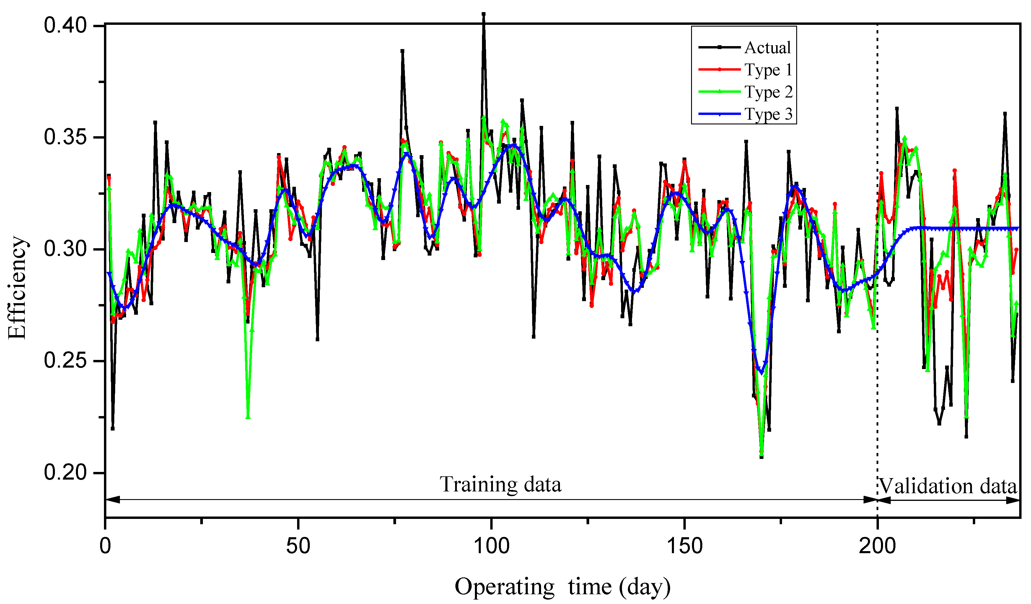
Therefore, the core step in the degradation failure model is to predict the performance parameters of the compressor unit based on the historical performance data. In fact, the changes in the unit’s performance parameters can be related to many factors, such as the unit’s performance degradation, operation, and environmental conditions. Therefore, the variables affecting the performance parameters should be considered in the prediction process. As such, a support-vector machine (SVM) for regression is utilized in this study to forecast the performance parameters of the compressor unit during the mission time, and a brief introduction to the SVM for regression is presented as follows:

The support-vector machine is a machine learning method proposed by Vapnik et al. [40]. It is based on statistical learning theory and the principle of structural risk minimization. Suppose that the training dataset has the basic form $\left\{({\mathit{x}}_1,y_1),({\mathit{x}}_2,y_2),\dots ,({\mathit{x}}_n,y_n)\right\}$, where ${\mathit{x}}_i\in R^n$ is the ith input vector of the n-dimensional samples, and $y_i\in R^1$ is the prediction target. The SVM for regression can then construct an optimized linear regression by mapping the input vector ${\mathit{x}}_i\in R^n$ to a high-dimensional feature space via nonlinear mapping $\varphi (\mathit{x})$, as expressed in Equation (6):

$$f(\mathit{x})=\mathit{w}\cdot \varphi (\mathit{x})+b$$

(6)

where f(x) is the regression function of SVM, w is the weight vector, and b is the bias term. In order to determine the w and b, the constrained optimization problem is formulated as follows:

$$\underset{\mathit{w},b}{\min }\left[\frac{1}{2}{\Vert \mathit{w}\Vert }^2+C{\displaystyle \sum _{i=1}^m({\xi }_i^{+}+{\xi }_i^{-})}\right]$$

(7)

$$s.t.\{\begin{array}{l}{y}_i-f({\mathit{x}}_i)\le \epsilon +{\xi }_{{}_i}^{+}\\ y_i-f({\mathit{x}}_i)\le \epsilon +{\xi }_{{}_i}^{-}\\ {\xi }_{{}_i}^{+},{\xi }_{{}_i}^{-}\ge 0,i=1,2,\dots ,n\end{array}$$

(8)

where C is the error penalty factor, ${\xi }_{{}_i}^{+}$ and ${\xi }_{{}_i}^{-}$ are the slack variables, $\epsilon$ is the precision parameter, n is the number of input samples, and y_i is the output vector for the ith input sample. By means of solving the optimization problem of Equations (7) and (8), Equation (6) can be rewritten as follows:

$$f(\mathit{x})={\displaystyle \sum _{i=1}^n\left({\alpha }_i-{\alpha }_i^{*}\right)}K(\mathit{x},{\mathit{x}}_i)+b$$

(9)

where ${\alpha }_i$ and ${\alpha }_i^{*}$ are the Lagrange multipliers, and $K(\mathit{x},{\mathit{x}}_i)=\varphi (\mathit{x})\cdot \varphi ({\mathit{x}}_i)$ is the kernel function.

Therefore, by implementing the SVM, the performance parameters of the compressor unit can be predicted over the mission time, and the reliability for the degradation failure can then be evaluated based on Equations (4) and (5). Moreover, the steps for determining the reliability function of the degradation failure can be concluded as follows:

Step 1: Data collection.

According to the performance characteristics of the compressor unit, one or more performance parameters are selected to reflect its health condition. Moreover, the corresponding historical operating data of this unit are collected, and are used to calculate the performance parameters.

Step 2: SVM for regression.

The regression model of the performance parameters is developed by the SVM, and the regression error between the actual and predicted performance parameter values is obtained. In the regression model, the input vector includes the operating time and the operating conditions, and the prediction target is the performance parameter of the compressor unit.

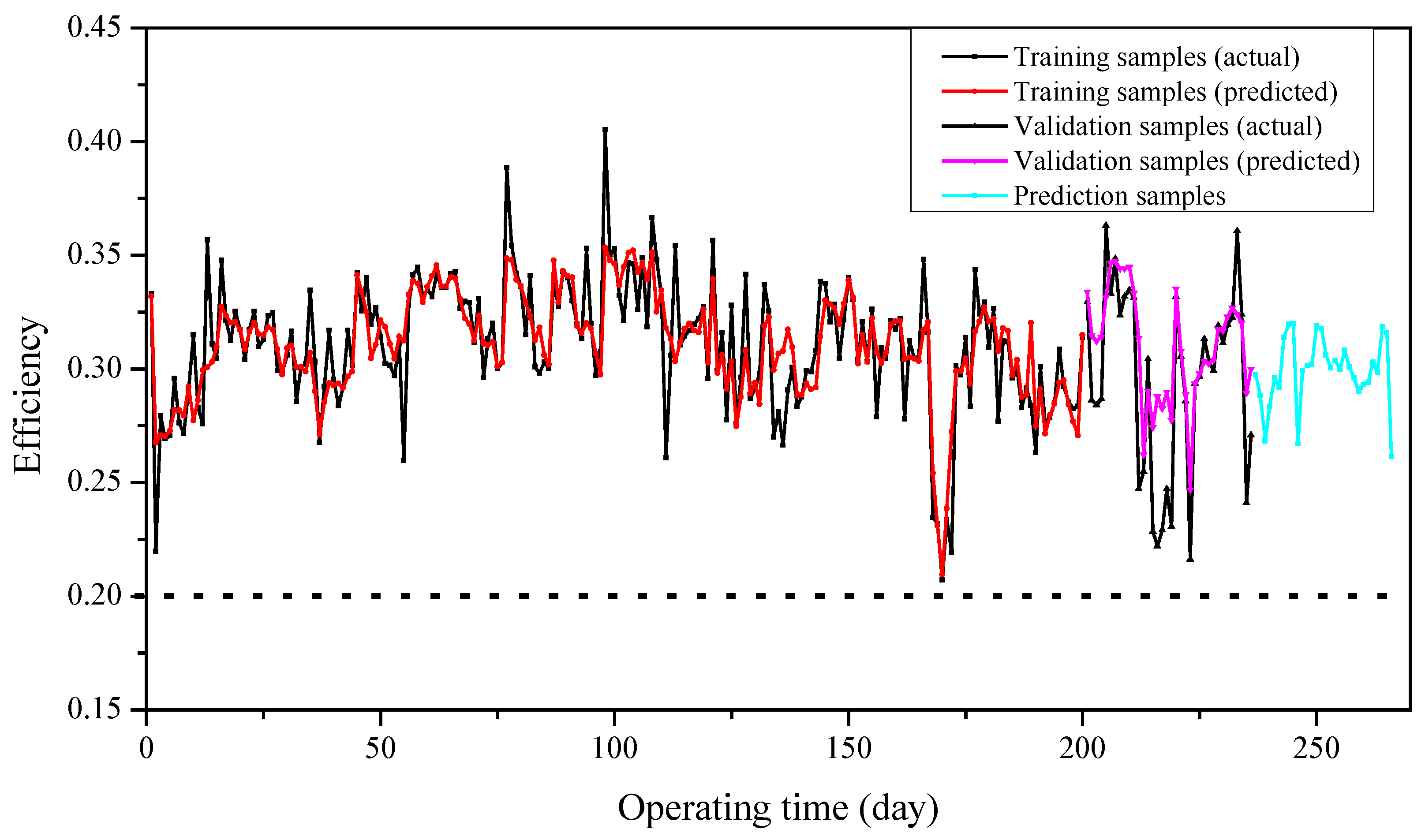
Step 3: Performance parameter prediction.

In this step, the mission time and the operating condition are specified, and the performance parameter of the compressor unit at the future time is predicted by the regression model developed in Step 2.

Step 4: Reliability calculation.

The critical threshold level is determined, and the reliability results for the degradation failure at each future discrete point of time, and over the mission time, are then calculated based on Equations (4) and (5).

2.3. Solving the Joint Probability

To consider the correlation of the two failure modes, the joint probability of the simultaneous occurrence of both catastrophic and degradation failure events during the mission time is solved in this section. Furthermore, the details required to solve the joint probability $\mathrm{Prob}\left[E_1\cap E_2\right]$ are presented as follows:

If both T_c and T_d follow the normal distribution with a correlation coefficient $\rho$, the multi-normal integral algorithm reported in Refs. [41,42] is employed to calculate the joint probability $\mathrm{Prob}\left[E_1\cap E_2\right]$, as shown in Equation (10):

$$\mathrm{Prob}\left[E_1\cap E_2\right]={\Phi }_2({\beta }_1,{\beta }_1,\rho )$$

(10)

where ${\Phi }_2(-,-,\rho )$ is the bivariate standard normal distribution function with a correlation coefficient ρ, which is the correlation coefficient between E₁ and E₂; ${\beta }_1$ and ${\beta }_2$ are the reliability indices for the events E₁ and E₂, respectively; ${\beta }_1={\Phi }^{-1}(P_c(t))$, ${\beta }_2={\Phi }^{-1}(P_d(t))$, and ${\Phi }^{-1}$ is the inverse function of the standard normal cumulative distribution function.

In fact, T_c and T_d can follow arbitrary distributions. The method of Nataf transformation, which can build a bridge between standard Gaussian space and the original probability space [43], is utilized to transform these original correlated random variables with the correlation coefficient $\rho$ into the normal correlated random variables with the correlation coefficient ${\rho }^{\prime }$. For simplicity, the relationship between $\rho$ and ${\rho }^{\prime }$ described in Ref. [43] is utilized in this study. Therefore, the scope of distributions includes the normal, uniform, shifted exponential, shifted Rayleigh, type-I largest value, type-I smallest value, Log-normal, gamma, type-II largest value, and type-III smallest value distributions.

For example, when the correlation of T_c and T_d with the correlation coefficient $\rho$ follows the Weibull distribution and normal distribution, respectively, the joint probability $\mathrm{Prob}\left[E_1\cap E_2\right]$ can be calculated as follows:

$$\mathrm{Prob}\left[E_1\cap E_2\right]={\Phi }_2({\beta }_1,{\beta }_1,{\rho }^{\prime })$$

(11)

$${\rho }^{\prime }=\{\begin{array}{l}\rho \cdot F\hspace{1em}0\le \rho <1\\ 1 \hspace{1em}\hspace{1em}\rho =1\end{array}$$

(12)

$$F=1.031-0.195{\delta }_j+0.328{\delta }_j^2$$

(13)

where ${\delta }_j$ is the coefficient of variation, and its range is from 0.1 to 0.5.

Moreover, the steps for solving the joint probability can be summarized as follows:

Step 1: The distributions of the time to catastrophic failure Tc and the time to degradation failure T_d are obtained as described in Section 2.1 and Section 2.2, respectively.

Step 2: The correlation coefficient ρ used in Equation (10) is calculated with the Nataf transformation.

Step 3: The values of β₁ and β₂ at the discrete points in time t₁, t₂,…, t_i are computed, and the joint probability of the catastrophic failure and degradation failure is then calculated based on Equation (10).

3. Case Study

In this section, the reliability of a natural gas compressor unit running in a natural gas transmission pipeline is analyzed using the proposed methodology. The compressor unit is the No. 2 unit at the ZW station located in China. In addition, the compressor unit is composed of a centrifugal compressor and a gas turbine, the models of which are RF2BB36 and RB211-GT62, respectively. The reliability of the compressor unit during the period from 24 August to 22 September in 2016 was predicted, and both the historical failure data and the performance data of the natural gas compressor unit were collected. More specifically, we also collected the historical failure data of both this unit and other units of the same type caused by catastrophic failures during the period from 1 January 2014 to 23 August 2016, as shown in

Table 2. The historical failure data derived from the catastrophic failures during the period from 1 January 2014 to 23 August 2016.

Compressor Unit	Failure Time	Time between Catastrophic Failures (Day)
No. 1 unit at ZW station	2014.5.9 (5:41) a)	--
	2014.5.23 (19:46)	14
	2014.11.12 (15:55)	173
	2015.10.22 (19:03)	333
No. 2 unit at ZW station	2015.5.20 (9:07)	---
	2015.8.16 (10:42)	88
	2015.8.24 (16:41)	8
	2016.1.23 (9:27)	152
	2016.3.25 (16:57)	62
	2016.6.16 (20:51)	83
	2014.4.14 (19:53)	---
No. 1 unit at JB station	2014.11.10 (16:30)	210
	2015.7.23 (12.56)	255
	2016.5.4 (9:32)	286
No. 2 unit at JB station	2015.7.15 (6:38)	---
	2015.9.24 (14:30)	71
	2015.11.9 (14:00)	46
	2016.2.24 (15:50)	106
	2016.6.21 (9:39)	118

^a) 2014.5.9 (5:41) denotes that the failure time was 5:41, 9 May 2014.

. The operating data—including volumetric rates and pressure ratios—from 1 January to 23 August in 2016 were measured, and the corresponding performance data were calculated, as presented in Figure 3. It should be noted that in addition to the repair period after the catastrophic failures, no other maintenance activity was carried out during the period of the data collection.

3.1. For Catastrophic Failures

From the data in Table 2, the time along the catastrophic failures can be determined. Moreover, the relationships between the time between failures (TBF), the time to repair (TTR), and the time to failure (TTF) are shown in Figure 4. Since the TTR is very short compared to the TTF for the units’ catastrophic failures based on the field data, the time to catastrophic failure T_c is approximately equal to the time between catastrophic failures in this case study, and the time to catastrophic failure T_c is listed in

Table 3. The time to catastrophic failure T_c of the compressor unit.

Order Number	Time to Catastrophic Failure (Days)	Order Number	Time to Catastrophic Failure (Days)	Order Number	Time to Catastrophic Failure (Days)
1	8	6	83	11	173
2	14	7	88	12	210
3	46	8	106	13	255
4	62	9	118	14	286
5	71	10	152	15	333

.

In order to choose the most suitable distribution to describe the time to catastrophic failure of the compressor unit T_c, the rank regression model proposed in Section 2.1 was utilized, and the frequency histogram and cumulative frequency histogram of the time to catastrophic failure are depicted in Figure 5. Moreover, the corresponding correlation coefficient ρ for each candidate distribution was then calculated, as listed in

Table 4. The correlation coefficients of the five candidate distributions.

Distribution	Normal Distribution	Log-Normal Distribution	Exponential Distribution	Weibull Distribution	Gumbel Distribution
Correlation coefficient	0.9941	0.9908	−0.9942	0.9982	−0.9980

. It can be seen that the Weibull distribution was the most suitable distribution in this case study. The corresponding parameters of the Weibull distribution were calculated. Moreover, Pearson’s chi-squared test was applied to test whether the time to catastrophic failure T_c matched the Weibull distribution. In fact, the Pearson’s chi-squared value in the case study was 0.345—less than the critical value when the significance level is 0.01. The test results show that the time to catastrophic failure T_c obeys the Weibull distribution. Therefore, the reliability and failure probability for the catastrophic failure up to time t are presented in Equations (14) and (15).

$$P_c(t)=1-\exp \left[-{(\frac{t}{\mu })}^{\sigma }\right]$$

(14)

$$R_c(t)=\exp \left[-{(\frac{t}{\mu })}^{\sigma }\right]$$

(15)

where t denotes the mission time in days, $\mu =152.3323$, and $\sigma =1.2324$.

3.2. For Degradation Failure

In this study, the efficiency of the compressor unit Eff, defined in Equation (16), was selected as the performance parameter to reflect the unit’s performance level.

$$Eff=\frac{H_o}{H_c}$$

(16)

where Eff represents the efficiency of the compressor unit; H_o is the energy obtained by the natural gas per day (kJ/day), which can be calculated by Equation (17); and H_c is the energy consumed by the compressor unit per day (kJ/day), which can be calculated based on the amount of natural gas consumption or power consumption by the compressor unit.

$$H_o=\{\frac{k}{k-1}\frac{Z_1+Z_2}{2}R{T}_{1}Q\rho ({\epsilon }_p{}^{\frac{m-1}{m}}-1)\hspace{1em}for\hspace{1em}\mathrm{centrifugal} \mathrm{compressor}\mathrm{unit}$$

(17)

where k is the specific heat ratio, Z₁ and Z₂ are the compressibility factors at the suction and discharge sides, respectively, R is the gas constant ($\mathrm{kJ}/(kg\cdot K)$), T₁ is the suction temperature K, Q is the volumetric flow rate (Nm³/day), $\rho$ is the gas density (kg/Nm³), ${\epsilon }_p$ is the pressure ratio $\raisebox{1ex}{$P_2$}\!\left/ \!\raisebox{-1ex}{$P_1$}\right.$, P₂ and P₁ are the pressure at the suction and discharge sides, respectively (Pa), and m is the isentropic exponent.

The SVM model described in Section 2.2 was utilized to predict the efficiency of the compressor unit throughout the mission time. As shown in Figure 5, the unit’s efficiency fluctuated randomly during operation rather than decreasing monotonically, due to the effect of the operating condition on the compressor unit’s efficiency. In fact, the changes in the unit’s performance parameters were related to the unit’s operating time and operating conditions. Moreover, from Equations (16) and (17), we know that the operating conditions are represented by the pressure ratio and volumetric flow rate. Therefore, the pressure ratio, the volumetric flow rate, and the cumulative operating time were selected as the input vectors of the SVM model.

In the case study, the training samples, validation samples, and prediction samples were the first 200 days (1 January to 18 July 2016), the 201st to 236th days (19 July to 23 August 2016), and the 237th to 266th days (24 August to 22 September 2016), respectively. Furthermore, aiming to illustrate the impact of the operating conditions on the precise forecasting of the performance parameters, the three different types of model inputs shown in

Table 5. The results of the three types of model inputs.

Type	Description	RMSE of the Training Data	RMSE of the Validation Data
Type 1	Both operating time and operating conditions are considered	0.0157	0.0279
Type 2	Only the operating conditions are considered	0.0167	0.0302
Type 3	Only the operating time is considered	0.0196	0.0431

were adopted when predicting the efficiency of the compressor unit. Thereafter, the quality of the forecast results of the three types was evaluated based on the root-mean-square error (RMSE), which can be calculated according to the following formula:

$$\mathrm{RMSE}=\sqrt{\frac{1}{N}{\displaystyle \sum _{i=1}^N{(\overline{Y}(t_i)-Y(t_i))}^2}}$$

(18)

where N is the number of data samples, $Y(t_i)$ is the actual value of the performance parameter with respect to time t_i, and $\overline{Y}(t_i)$ is the prediction value of the performance parameter.

In Table 5, a summary of the RMSE of the training data and validation data for the three types of model inputs is presented, and the comparisons of the predicted values and actual values are shown in Figure 6. One can observe that the RMSE of the first type of model input is the smallest among the three types, and the predicted values are consistent with the actual values in both the training data and the validation data. Moreover, the assessment results indicate the significant impact of the operating conditions on the precise forecasting of the performance parameter.

Moreover, a scatterplot of the prediction error is shown in Figure 7. The prediction error ε is assumed to represent the random variables of normal distribution, namely, $\epsilon \sim N(\mu ,{\sigma }^2)$, $\mu =3.535\times {10}^{-3}$, and $\sigma =2.011\times {10}^{-2}$. The Gaussian kernel function is adopted in the SVM model.

According the developed prediction model, once the operating conditions and operating time are specified, the efficiency of the compressor unit can be predicted, and the predicted values of the efficiency are shown in Figure 8. It should be noted that the future operating conditions of the compressor are determined by the future gas transmission tasks. Furthermore, the failure probability functions of the degradation failure for each time, and for a specific period of time, are then predicted based on Equations (4) and (5), respectively. However, due to the lack of a large amount of empirical information and experimental data, the failure threshold D_f is difficult to directly determine. In the case, D_f = 0.215 was assumed as the critical threshold of the compressor unit. Moreover, in order to investigate the sensitivity of the threshold to the reliability, three different threshold levels (high level, D_f = 0.23; medium level, D_f = 0.215; low level, D_f = 0.21) were considered, and the results of the reliability assessment are presented in Figure 9. The results show that the failure threshold has a great effect on the reliability of the degradation failure; thus, the determination of an appropriate threshold plays a key role in the degradation failure model.

3.3. Reliability Assessment of the Compressor Unit from a Comprehensive Perspective

In this section, the reliability functions of the catastrophic failure and degradation failure are integrated to assess the reliability of the compressor unit from a comprehensive perspective, and both their correlation and competitiveness are considered. As mentioned above, the time to catastrophic failure follows the Weibull distribution, while the time to degradation failure is assumed to follow the normal distribution. Moreover, the correlation coefficient between catastrophic failure and degradation failure is assumed to be ρ. The Nataf transformation was utilized to transform these original correlated random variables with the correlation coefficient ρ to normal correlated random variables with the correlation coefficient ρ’, and the calculation formulae shown in Equations (11) and (12) were used to calculate the correlation coefficient ${\rho }^{\prime }$ after the aforementioned Nataf transformation. The range of ${\delta }_j$ is from 0.1 to 0.5, and in this case study we set ${\delta }_j$ as 0.3; thus, the relationship between ${\rho }^{\prime }$ and $\rho$ can be shown as follows:

$${\rho }^{\prime }=\{\begin{array}{l}1.00202\times \rho \hspace{1em}0\le \rho <1\\ 1\hspace{1em}\hspace{1em}\hspace{1em}\hspace{1em} \rho =1\end{array}$$

(19)

However, the information of the correlation coefficient between catastrophic failure and degradation failure is also lacking. Four levels of the correlation coefficient (ρ = 0, 0.3, 0.7, and 1) were employed to calculate the reliability of the compressor unit. The sensitivity of the correlation to the reliability was investigated, and these scenarios are summarized in

Table 6. The correlation coefficients for four scenarios.

Scenario	$\mathit{\rho }$	${\mathit{\rho }}^{\prime }$
1	0	0
2	0.3	0.300606
3	0.7	0.701414
4	1	1

.

Both the degradation failure and the catastrophic failure of the natural gas compressor unit might incur high costs and/or safety hazards. For this reason, preventive maintenance typically has a high significance in terms of cost and safety. Hence, it is especially necessary to accurately evaluate the reliability of the natural gas compressor unit. Figure 10 shows the assessment results of the reliability for all levels of the correlation coefficient. The figure indicates that only considering one of the modes—catastrophic failure or degradation failure—will cause the reliability evaluation result to be inconsistent with the actual situation. Moreover, the correlation of the two failure modes has significate impacts on the unit’s reliability. The reliability of the compressor unit increases with the increase in the correlation coefficient. The assumption of mutually independent failure modes will lead to a conservative prediction due to neglect of the probability of joint failure. Application of the data-driven methods helps to handle the reliability analysis of the natural gas compressor unit.

Moreover, as a result of catastrophic failures, the reliability of the compressor unit drops rapidly over the mission time. However, this does not mean that the compressor unit has low availability. The reason for this is that the repair time corresponding to the catastrophic failure is relatively short, ensuring that the recovery can be started quickly after the catastrophic failure occurs. Hence, the availability of the compressor unit can be maintained at a high level in actual operation.

4. Conclusions and Future Work

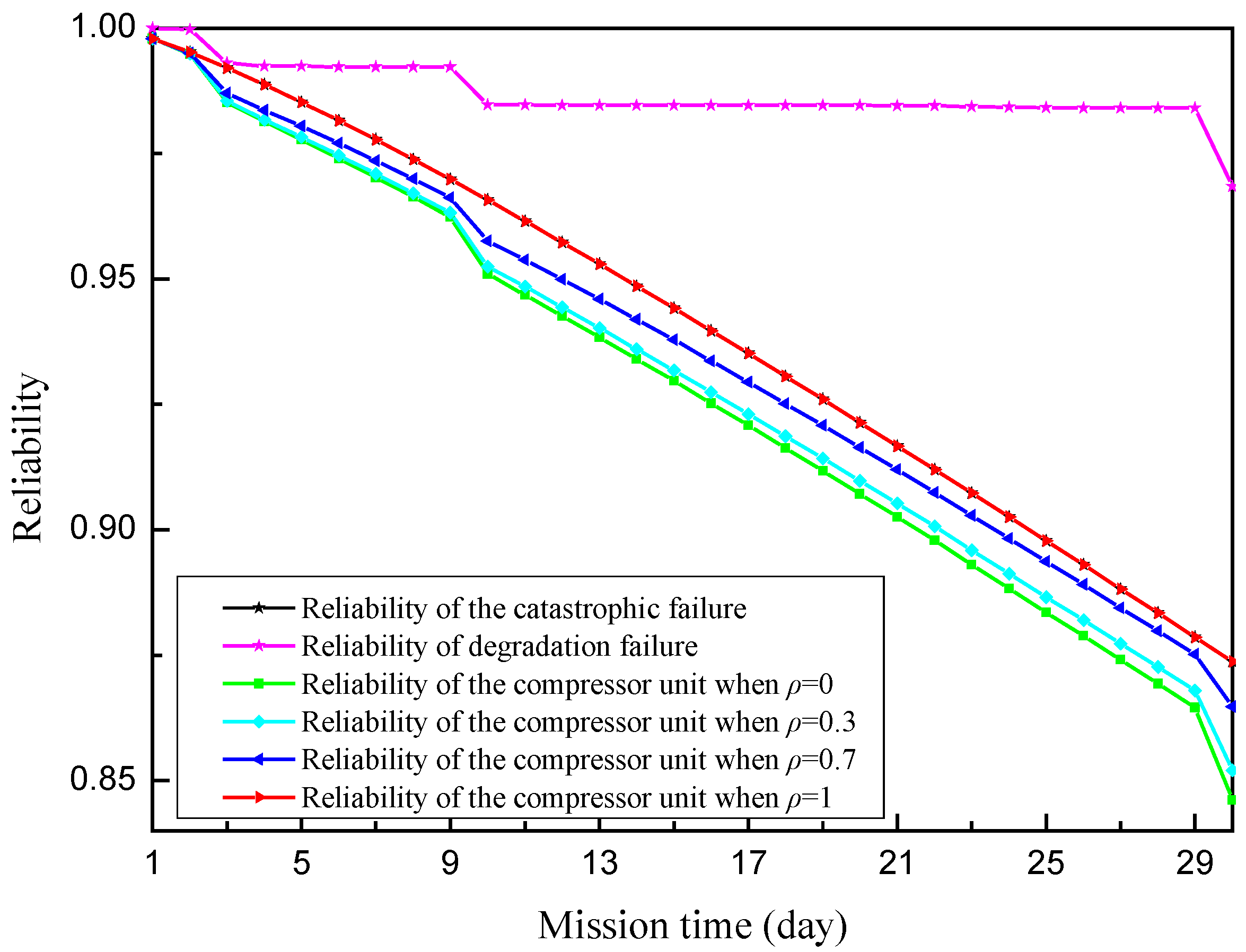
This paper proposed a data-driven methodology to evaluate and predict the reliability of compressor units from a comprehensive perspective, and both the historical failure data and the performance data of the natural gas compressor unit were used. Moreover, we also considered the effects of the external environment and operating conditions on the reliability of the compressor unit in this study, and built the reliability functions for the catastrophic and degradation failures to develop our data-driven methodology. Thereafter, the reliability of the compressor unit was assessed by combining the reliability functions of the catastrophic and degradation failures, and the competitiveness and correlation of these two failure modes were taken into account.

To demonstrate the feasibility of our proposed methodology, a case study of a running centrifugal compressor driven by a gas turbine was conducted. Furthermore, the impact of the operating conditions on the predictive precision of the performance data and the sensitivity of both the degradation threshold and the correlation level to the reliability were investigated in the case study.

Evidently, our methodology also has several limitations. These limitations are mainly related to the insufficient consideration of the failure modes of the compressor units, as well as the impact of the maintenance and environmental conditions. Hence, further efforts should focus on describing the failure modes more realistically, and considering the factors of the maintenance and environmental conditions, along with the influence of the driving gas turbine on the compressor’s operating data.

References

1. Hong, B.; Li, X.; Di, G.; Li, Y.; Liu, X.; Chen, S.; Gong, J. An integrated MILP method for gathering pipeline networks considering hydraulic characteristics. Chem. Eng. Res. Des. 2019, 152, 320–335. [Google Scholar] [CrossRef]
2. Lv, X.-F.; Zuo, J.-W.; Liu, Y.; Zhou, S.-D.; Lu, D.-Y.; Yan, K.-L.; Shi, B.-H.; Zhao, H.-J. Experimental study of growth kinetics of CO2 hydrates and multiphase flow properties of slurries in high pressure flow systems. RSC Adv. 2019, 9, 32873–32888. [Google Scholar] [CrossRef] [PubMed] [Green Version]
3. Lv, X.F.; Shi, B.H.; Zhou, S.D.; Peng, H.P.; Lei, Y.; Yu, P.F. Study on the growth rate of natural gas hydrate in water-in-oil emulsion system using a high-pressure flow loop. RSC Adv. 2018, 8, 36484–36492. [Google Scholar] [CrossRef] [Green Version]
4. Zapukhliak, V.; Poberezhny, L.; Maruschak, P.; Grudz, V., Jr.; Stasiuk, R.; Brezinová, J.; Guzanová, A. Mathematical Modeling of Unsteady Gas Transmission System Operating Conditions under Insufficient Loading. Energies 2019, 12, 1325. [Google Scholar] [CrossRef] [Green Version]
5. Yu, W.; Song, S.; Li, Y.; Min, Y.; Huang, W.; Wen, K.; Gong, J. Gas supply reliability assessment of natural gas transmission pipeline systems. Energy 2018, 162, 853–870. [Google Scholar] [CrossRef]
6. Weihe, H.; Honglong, Z.; Mingfei, L. Development history and prospect of oil & gas storage and transportation industry in China. Oil Gas Storage Transp. 2019, 38, 1–11. [Google Scholar]
7. Yu, W.; Gong, J.; Song, S.; Huang, W.; Li, Y.; Zhang, J.; Hong, B.; Zhang, Y.; Wen, K.; Duan, X. Gas supply reliability analysis of a natural gas pipeline system considering the effects of underground gas storages. Appl. Energy 2019, 252, 113418. [Google Scholar] [CrossRef]
8. Yu, W.; Huang, W.; Liu, H.; Wang, K.; Wen, K.; Gong, J.; Zhang, M. A systematic method for assessing the operating reliability of the underground gas storage in multiple salt caverns. J. Energy Storage 2020, 31, 101675. [Google Scholar] [CrossRef]
9. Tran, T.H.; French, S.; Ashman, R.; Kent, E. Impact of compressor failures on gas transmission network capability. Appl. Math. Model. 2018, 55, 741–757. [Google Scholar] [CrossRef] [Green Version]
10. Yu, W.; Wen, K.; Min, Y.; He, L.; Huang, W.; Gong, J. A methodology to quantify the gas supply capacity of natural gas transmission pipeline system using reliability theory. Reliab. Eng. Syst. Saf. 2018, 175, 128–141. [Google Scholar] [CrossRef]
11. Li, B.; Zhang, L.; Yang, X.; Dong, X.; Huang, E.; Li, X.; Wei, X. Reliability of gas turbine driven compressor sets for gas pipelines. Oil Gas Storage Transp. 2016, 35, 920–923. [Google Scholar]
12. Li, J. Reliability Analysis of the Natural Gas Compressor; Southwest Petroleum Institute: Chengdu, China, 2005. [Google Scholar]
13. Guo, X.; Zhang, L.; Liang, W.; Feng, H. A reliability analysis method for compressors based on FMEA/FEM. Oil Gas Storage Transp. 2016, 35, 1042–1049. [Google Scholar]
14. Chen, P. Method of Reliability Analysis and Digital Study for Reciprocating Compressor. Ph.D. Thesis, Northeastern University, Boston, MA, USA, 2009. [Google Scholar]
15. Woo, S.; Pecht, M.; O’Neal, D.L. Reliability design and case study of a refrigerator compressor subjected to repetitive loads. Int. J. Refrig.-Rev. Int. Froid. 2009, 32, 478–486. [Google Scholar] [CrossRef]
16. Woo, S.-W.; Pecht, M.; O’Neal, D.L. Reliability design and case study of the domestic compressor subjected to repetitive internal stresses. Reliab. Eng. Syst. Saf. 2020, 193, 106604. [Google Scholar] [CrossRef]
17. Chang, M.S.; Park, J.W.; Choi, Y.M.; Park, T.K.; Choi, B.O.; Shin, C.J. Reliability evaluation of scroll compressor for system air conditioner. J. Mech. Sci. Technol. 2016, 30, 4459–4463. [Google Scholar] [CrossRef]
18. Ye, Z.-S.; Xie, M. Stochastic modelling and analysis of degradation for highly reliable products. Appl. Stoch. Model. Bus. Ind. 2015, 31, 16–32. [Google Scholar] [CrossRef]
19. Yang, Y. Research on reliability Evaluation for Mechanical Products Based on Degradation Modelling. Ph.D. Thesis, University of Electronic Science and Technology of China, Chengdu, China, 2016. [Google Scholar]
20. Crk, V. Reliability assessment from degradation data. In Proceedings of the Annual Reliability and Maintainability Symposium 2000 Proceedings International Symposium on Product Quality and Integrity (Cat No00CH37055), Los Angeles, CA, USA, 24–27 January 2000; pp. 155–161. [Google Scholar]
21. Huitian, L.; Kolarik, W.J.; Lu, S.S. Real-time performance reliability prediction. IEEE Trans. Reliab. 2001, 50, 353–357. [Google Scholar] [CrossRef]
22. Gebraeel, N.Z.; Lawley, M.A.; Li, R.; Ryan, J.K. Residual-life distributions from component degradation signals: A Bayesian approach. IIE Trans. 2005, 37, 543–557. [Google Scholar] [CrossRef]
23. Zhou, D.; Zhang, H.; Weng, S. A novel prognostic model of performance degradation trend for power machinery maintenance. Energy 2014, 78, 740–746. [Google Scholar] [CrossRef]
24. Zhou, D.; Yu, Z.; Zhang, H.; Weng, S. A novel grey prognostic model based on Markov process and grey incidence analysis for energy conversion equipment degradation. Energy 2016, 109, 420–429. [Google Scholar] [CrossRef]
25. Li, Y.G.; Nilkitsaranont, P. Gas turbine performance prognostic for condition-based maintenance. Appl. Energy 2009, 86, 2152–2161. [Google Scholar] [CrossRef]
26. Puggina, N.; Venturini, M. Development of a Statistical Methodology for Gas Turbine Prognostics. J. Eng. Gas Turbines Power 2011, 134, 22401. [Google Scholar] [CrossRef]
27. Venturini, M.; Puggina, N. Prediction Reliability of a Statistical Methodology for Gas Turbine Prognostics. J. Eng. Gas Turbines Power 2012, 134, 101601. [Google Scholar] [CrossRef]
28. Safiyullah, F.; Sulaiman, S.A.; Naz, M.Y.; Jasmani, M.S.; Ghazali, S.M.A. Prediction on performance degradation and maintenance of centrifugal gas compressors using genetic programming. Energy 2018, 158, 485–494. [Google Scholar] [CrossRef]
29. Ye, Z.-S.; Chen, N.; Shen, Y. A new class of Wiener process models for degradation analysis. Reliab. Eng. Syst. Saf. 2015, 139, 58–67. [Google Scholar] [CrossRef]
30. Dong, Q.; Cui, L. A study on stochastic degradation process models under different types of failure Thresholds. Reliab. Eng. Syst. Saf. 2019, 181, 202–212. [Google Scholar] [CrossRef]
31. Peng, W.; Li, Y.-F.; Yang, Y.-J.; Huang, H.-Z.; Zuo, M.J. Inverse Gaussian process models for degradation analysis: A Bayesian perspective. Reliab. Eng. Syst. Saf. 2014, 130, 175–189. [Google Scholar] [CrossRef]
32. Che, H.; Zeng, S.; Guo, J.; Wang, Y. Reliability modeling for dependent competing failure processes with mutually dependent degradation process and shock process. Reliab. Eng. Syst. Saf. 2018, 180, 168–178. [Google Scholar] [CrossRef]
33. Deng, A. Research on Reliability Technology of High-Reliability and Long-Lifetime Products. Ph.D. Thesis, National University of Defense Technology, Changsha, China, 2006. [Google Scholar]
34. Tang, D.; Yu, J.; Chen, X.; Makis, V. An optimal condition-based maintenance policy for a degrading system subject to the competing risks of soft and hard failure. Comput. Ind. Eng. 2015, 83, 100–110. [Google Scholar] [CrossRef]
35. Wang, Y.; Pham, H. Dependent competing-risk degradation systems. In Safety and Risk Modeling and Its Applications; Springer: Berlin/Heidelberg, Germany, 2011; pp. 197–218. [Google Scholar]
36. Calixto, E. Gas and Oil Reliability Engineering: Modeling and Analysis; Gulf Professional Publishing: London, UK, 2016. [Google Scholar]
37. Yu, W.; Zhang, J.; Wen, K.; Huang, W.; Min, Y.; Li, Y.; Yang, X.; Gong, J. A novel methodology to update the reliability of the corroding natural gas pipeline by introducing the effects of failure data and corrective maintenance. Int. J. Press. Vessel. Pip. 2019, 169, 48–56. [Google Scholar] [CrossRef]
38. Deng, A.; Chen, X.; Zhang, C.; Wang, Y. Reliability assessment based on Performance degradation data. J. Astronaut. 2006, 27, 546–552. [Google Scholar]
39. Zhong, Q.; Zhang, Z.; Liang, S. Reliabiity analysis approach based on multivariate degradation data. Syst. Eng.-Theory Pract. 2011, 31, 544–551. [Google Scholar]
40. Vapnik, V. The Nature of Statistical Learning Theory; Springer Science & Business Media: Berlin/Heidelberg, Germany, 2013. [Google Scholar]
41. Kang, W.-H.; Song, J. Evaluation of multivariate normal integrals for general systems by sequential compounding. Struct. Saf. 2010, 32, 35–41. [Google Scholar] [CrossRef]
42. Gong, C.; Zhou, W. Improvement of equivalent component approach for reliability analyses of series systems. Struct. Saf. 2017, 68, 65–72. [Google Scholar] [CrossRef]
43. Liu, P.-L.; Der Kiureghian, A. Multivariate distribution models with prescribed marginals and covariances. Probabilistic Eng. Mech. 1986, 1, 105–112. [Google Scholar] [CrossRef]
Figure 1. Schematic diagrams of the two failure modes.
Energies 15 03557 g001
Figure 2. Block diagram of the stages of reliability analysis of the natural gas compressor.
Energies 15 03557 g002
Figure 3. The performance parameters and operating time for the 2# compressor unit from 1 January to 23 August in 2016.
Energies 15 03557 g003
Figure 4. The schematic of the relationships between the TBF, TTR, and TTF.
Energies 15 03557 g004
Figure 5. The frequency histogram and the cumulative frequency histogram of the time to catastrophic failure and the most suitable distribution.
Energies 15 03557 g005
Figure 6. The comparison among the three types of model inputs.
Energies 15 03557 g006
Figure 7. Prediction error of the SVM method.
Energies 15 03557 g007
Figure 8. The prediction results of the SVM.
Energies 15 03557 g008
Figure 9. The reliability for the degradation failure under different threshold levels.
Energies 15 03557 g009
Figure 10. The change process of the reliability of the compressor unit.
Energies 15 03557 g010