Influence of the Catenary Distributed Parameters on the Resonance Frequencies of Electric Railways Based on Quantitative Calculation and Field Tests

Abstract

High-order harmonic resonance is a key issue in the traction power supply systems (TPSS) of electric railways for safe operation. The effective evaluation of the resonance frequency is critical for taking measures to suppress harmonic resonance. In this paper, the influence of the distributed parameters of traction networks on resonance frequencies based on accurate calculation is proposed. The quantitative assessments of the distributed impedance and admittance are investigated. Furthermore, the theoretical calculation is directly verified using field tests at a high voltage level equal to 25 kV. The results show that the resonance frequencies of the TPSS are mainly affected by the distributed parameters, including the self-admittance and self-impedance of the contact wires, and the self-admittance of the positive feeders. In addition, the admittance connected in parallel has a greater effect than the series-connected impedance. The calculation method is also adapted to TPSS connected to renewable energy.

1. Introduction

In current electric railways, the high-order harmonic resonance (HHR) of traction power supply systems (TPSS) is a great technical challenge due to its complex characteristics. The study of HHR has attracted much attention from researchers in many countries, such as China, Britain, Italy, Korea, New Zealand, Spain, and Thailand [1,2,3,4,5,6,7,8,9,10]. In order to suppress the HHR, the accurate estimation of the resonance frequencies of electric railways is essential for adapting measures, e.g., passive filter installation along the railway, electrical parameters, and control method adjustments of the traction converters [5,11,12,13,14,15]. Therefore, forecasting the resonance frequencies and investigating the influence of different factors are necessary. In [16], Holtz studied the influence mechanism of track topography and traction vehicle position changes on the harmonics of overhead power supply systems based on the wave propagation approach. In [17], the influence of soil was considered, and distributed construction and soil modeling were established. However, the simplified track topography is significantly different from present electric railways. Dolara built simulation models to study the harmonic penetration and resonance frequencies [18], and showed that the resonance frequency is affected by the three-phase high-voltage power system when the traction system is coupled with this power system. However, the detailed/corrected parameters of railways and power systems are required in this model, which are not suitable in some countries. In [19], the harmonic distribution model of the track traction current of an AC electrified railway was established, and it proved that the harmonic current distribution depends on the distance among the power supply substation, the rail-to-earth conductance, and the train locations in the feeder area. Andrea studied the resonance conditions at the interface of the on-board pantograph, and proposed a scheme of on-line measurement for real-time implementation [20]. The model of the power supply lines was not considered in [20], such as the catenary. In [21], external balancing devices, i.e., a static VAR compensator (SVC), were installed in a 1 × 25 kV railway, and the effect of SVC on harmonic resonances was studied. Nevertheless, the commonly used 2 × 25 kV TPSS was not considered. Catenary length plays an important role in determining resonance frequencies. Hence, in [2,22,23], simulations with PSCAD or RT-lab were carried out to detect the resonance points of the TPSS. However, catenary parameters with respect to frequency were not considered. More precisely, the skin effect and proximity effect were neglected. In [24,25], the influence of the skin effect was studied, and the calculation formula of impedance in a conductor was given. However, they are not directly applicable to the catenary and rail of TPSS. Considering the influence of frequency, papers [26,27] simulated the variation of the rail impedance with frequency by different methods. The characteristics of rail impedance with a frequency under 50–650 Hz frequencies or audiofrequency conditions were measured, respectively [28,29]. However, the methods of these articles have not been tested in the field. In addition, none of the abovementioned studies were directly verified by field tests in actual railways. In [2], a step-down laboratory test with a low voltage level, at 220 V, was carried out. However, there is still a huge gap between the low-voltage validation and the real system with the rated voltage at 25 kV.

Compared with the literature, this paper explores the relationship between the catenary distributed parameters and the resonance frequencies of a 25 kV autotransformer-fed (AT-fed) electric railway over a wide frequency range of ~4000 Hz.

Table 1. Comparison with other studies.

Literatures	Main Contribution	Methodology
[2]	Proposed impact of catenary length on harmonic resonance frequency	Simulation and tests at 220 V
[16]	Proposed impact of traction vehicles and feeding substations on harmonic resonance frequency	Simulation with a simple two-track model
[17]	Established the distributed construction and soil modeling.	Simulation in Modelica simulation Language
[18]	Proposed impact of power system line, track circuits on harmonic resonance frequency on harmonic resonance frequency	Simulation with a coupled track model
[19]	Established harmonic distribution model of track traction current of AC electrified railway	Simulation with Mathematical model
[20]	Proposed a scheme of on-line measurement suitable for real-time implementation	Field test and data analysis
[21]	Proposed impact of external balancing equipment on harmonic resonance frequency	Tectorial analysis and calculation
[22]	Proposed impact of catenary length and load demand on harmonic resonance frequency	Simulation
[23]	Proposed impact of catenary length and ATs on harmonic resonance frequency	Simulation
This paper	Proposed impact of distributed parameters of all the contact wires on harmonic resonance frequency	Calculations and validations by field tests at 25 kV

summarizes the current research and the contributions in this paper.

The main contributions of this paper are summarized as follows:

(a)

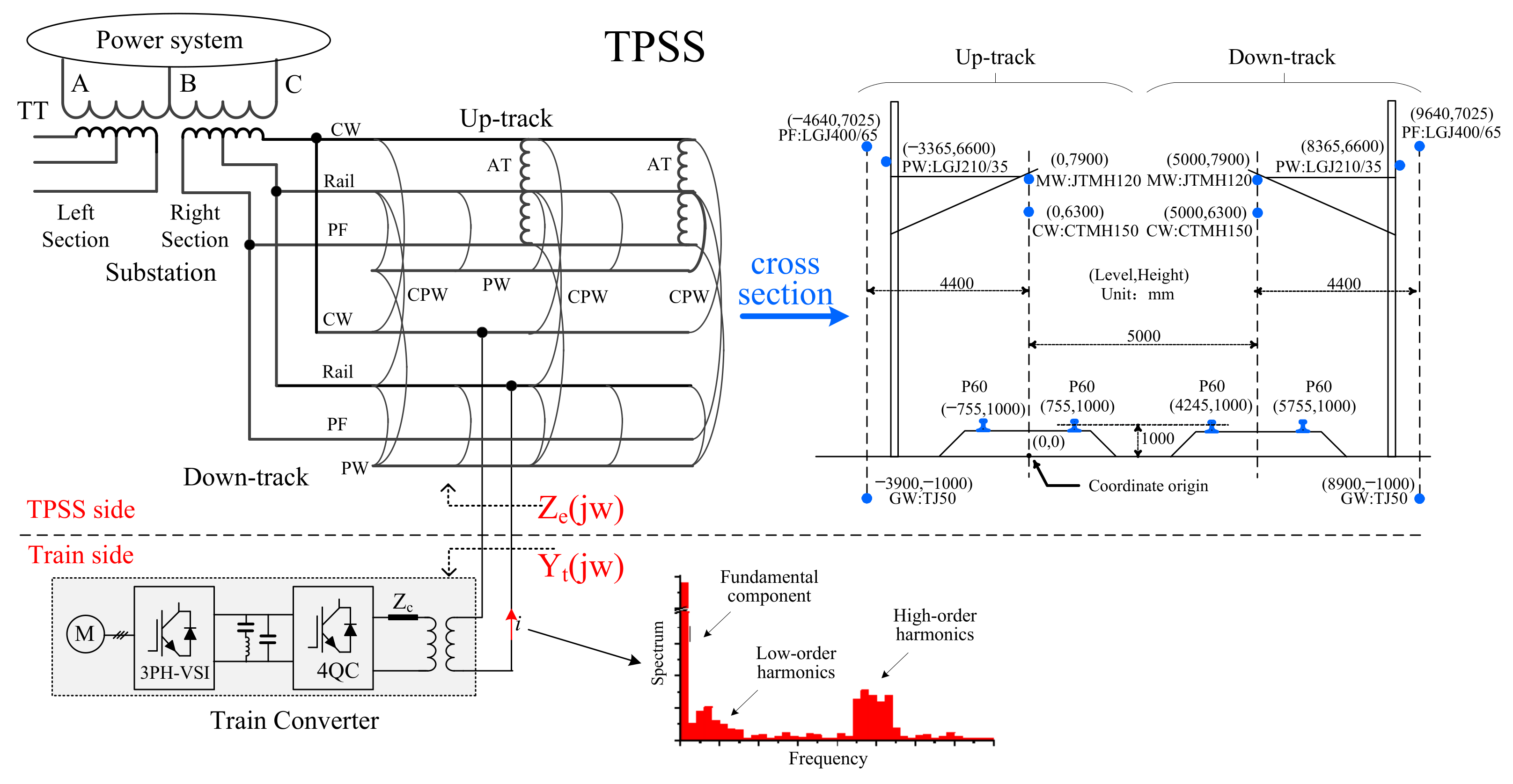
The influence of the catenary distributed parameters on the resonance frequencies is quantitatively and comprehensively studied. The indicator, defined as a marginal utility (MU), is proposed in order to determine the primary and subordinate factors. As shown in Figure 1, a multiconductor transmission system is applied in TPSS. This system is composed of contact wires (CWs), messenger wires (MWs), protective wires (PWs), positive feeders (PFs), rails, and ground wires (GWs). These practical installations and the geometrical configuration (e.g., viaduct, tunnel, and railroad bed) determine the catenary distributed parameters, i.e., the catenary admittance and impedance per unit length. Therefore, the resonance frequencies of a railway can hardly be estimated accurately without the global consideration of the distributed parameters. In this paper, a 10-conductor model of an actual AT-fed railway is developed. Then, all of the elements of the 10-conductor model are quantificationally investigated by MU. Research on the connection of renewable energy power generation systems to electrified railways has been carried out [30,31]. This model can also be applied to electrified railways with renewable energy by making an equivalent of renewable energy to an impedance at the access point.

(b)

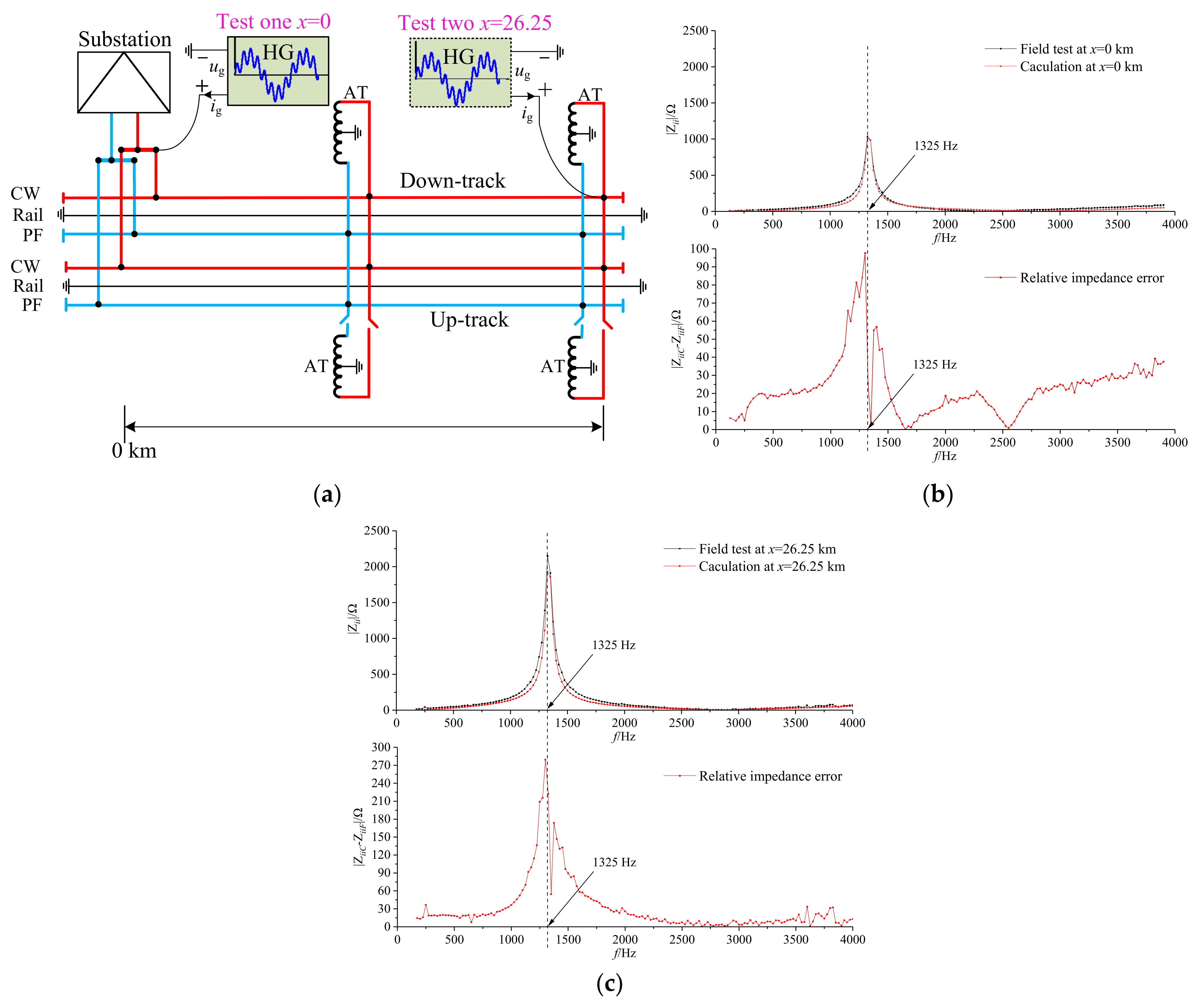
The 10-conductor model calculation results and related analysis are guaranteed by direct field tests in an actual AT-fed railway at 25 kV. As shown in Table 1, the literature can provide different conclusions about the resonance frequency’s changing rules. However, it should be noted that the analysis results are directly related to the accuracy and correctness of the calculations. Most of the current studies are based on simulation tests without sufficient experiments or actual data from real systems. The errors introduced by the model parameters and nonlinearity in the high-frequency range cannot be evaluated. For example, many software tools and calculation models mainly deal with cylindrical conductors [32,33]. It is difficult to calculate the impedance of irregularly shaped conductors (e.g., the CW and rail, as presented in Figure 2) over a large frequency range, considering both the spiraling effect and skin effect. The internal resistance and inductance of the rail by the finite element method is proposed in [26], while other factors, such as the ground circuit, are neglected. In addition, if resistor-inductor-capacitor-based impedance networks with lumped parameters are used to build models, they are convenient to implement. However, considerable error may be introduced because the actual power supply section is long enough (e.g., ~25 km for actual electric railways) compared with the electromagnetic wavelength at several thousand hertz. In this paper, the system model and algorithm used to calculate the resonance frequency are presented in Section 2. The calculation results are validated using direct field tests at 25 kV, which have been reported in our previous works [34,35]. The validation results ensure the calculation accuracy of this paper, which lays a solid foundation to evaluate the influence of distributed parameters. The test can also provide necessary information and overcome the lack of reliable data for actual systems. Based on the substantial measured data and an improved model [36], this paper investigates the effect of distributed parameters on resonance frequencies.

The remainder of this paper is organized as follows. In Section 2, the multiconductor transmission line (MTL) model and the calculation process are presented in detail. Then, the effectiveness of the model is verified using theoretical analysis and field tests. In Section 3, the distributed admittance and impedance per unit length are analyzed. The contribution of each distributed parameter to the resonance frequencies is quantitatively assessed. Finally, conclusions are drawn in Section 4.

2. Resonance Frequency Calculation Method

2.1. Calculation of the Input Impedance

Overall, the TPSS can be regarded as a chain network, as shown in Figure 3. The chain network is represented by the series-connected impedance components Z_i (i = 1, 2, ···, N−1), parallel-connected admittance components Y_i, and injected current I_i(i = 1, 2, ···, N). The voltage at node i is denoted as V_i (i = 1, 2, ···, N). If the catenary system is made up of m wires (for example, in Figure 1, m is 14, as shown in blue), Z_i and Y_i are m × m matrices, and I_i and V_i are m × 1 vectors.

The nodal voltage equation of this chain network is given by

YV = I,

(1)

where Y, V, and I are

$$\left\{\begin{array}{l}Y=\left[\begin{array}{cccc}{Y}_1+Z_1^{-1}& -Z_1^{-1}& & \\ -Z_1^{-1}& Z_1^{-1}+Y_2+Z_2^{-1}& & \\ & -Z_2^{-1}& \ddots & -Z_{N-1}^{-1}\\ & & & Z_{N-1}^{-1}+Y_N\end{array}\right]\\ V={\left[\begin{array}{ccc}{V}_1& V_1& \begin{array}{cc}\dots & V_N\end{array}\end{array}\right]}^T\\ I={\left[\begin{array}{ccc}{I}_1& I_1& \begin{array}{cc}\dots & I_N\end{array}\end{array}\right]}^T\end{array}\right.,$$

(2)

If I is not independent of V, (1) is a nonlinear equation. Here, the Picard iteration method is used to solve (1).

Assuming that

$$F(V)=YV-I(V),$$

(3)

The solution of $F(V)=0$ can be given by

$$V^{\left(k\right)}=Y^{-1}{I}^{(k-1)}.$$

(4)

The matrix form of (4) is defined as

$$\left[\begin{array}{c}{V}_1^{(k)}\\ V_2^{(k)}\\ ⋮\\ V_{N-1}^{(k)}\\ V_N^{(k)}\end{array}\right]={\left[\begin{array}{ccccc}{M}_1& D_1& & & \\ D_1& M_2& D_2& & \\ & \ddots & \ddots & \ddots & \\ & & D_{N-2}& M_{N-1}& D_{N-1}\\ & & & D_{N-1}& M_N\end{array}\right]}^{-1}\left[\begin{array}{c}{I}_1^{(k-1)}\\ I_2^{(k-1)}\\ ⋮\\ I_{N-1}^{(k-1)}\\ I_N^{(k-1)}\end{array}\right]$$

(5)

where

$$\left\{\begin{array}{l}{M}_1=Y_1+Z_1^{-1}\hfill \\ M_i=Z_{i-1}^{-1}+Y_i+Z_i^{-1}\left(i=2,3,\cdots ,N-1\right)\hfill \\ M_N=Z_{N-1}^{-1}+Y_N\hfill \\ D_i=-Z_i^{-1}\left(i=1,2,\cdots ,N-1\right)\hfill \end{array}\right.,$$

(6)

The LU factorization of Y is described as

$$Y=\left[\begin{array}{ccccc}1& & & & \\ C_2& 1& & & \\ & \ddots & \ddots & & \\ & & C_{N-1}& 1& \\ & & & C_N& 1\end{array}\right]\left[\begin{array}{ccccc}{A}_1& E_1& & & \\ & A_2& E_2& & \\ & & \ddots & \ddots & \\ & & & A_{N-1}& E_{N-1}\\ & & & & A_N\end{array}\right],$$

(7)

Assuming that

$$\left[\begin{array}{ccccc}{A}_1& E_1& & & \\ & A_2& E_2& & \\ & & \ddots & \ddots & \\ & & & A_{N-1}& E_{N-1}\\ & & & & A_N\end{array}\right]\left[\begin{array}{c}{V}_1^{(k)}\\ V_2^{(k)}\\ ⋮\\ V_{N-1}^{(k)}\\ V_N^{(k)}\end{array}\right]=\left[\begin{array}{c}{h}_1^{(k-1)}\\ h_2^{(k-1)}\\ ⋮\\ h_{N-1}^{(k-1)}\\ h_N^{(k-1)}\end{array}\right],$$

(8)

and substituting (7) and (8) into (5) yields

$$\left[\begin{array}{ccccc}1& & & & \\ C_2& 1& & & \\ & & \ddots & \ddots & \\ & & C_{N-1}& 1& \\ & & & C_N& 1\end{array}\right]\left[\begin{array}{c}{h}_1^{(k-1)}\\ h_2^{(k-1)}\\ ⋮\\ h_{N-1}^{(k-1)}\\ h_N^{(k-1)}\end{array}\right]=\left[\begin{array}{c}{I}_1^{(k-1)}\\ I_2^{(k-1)}\\ ⋮\\ I_{N-1}^{(k-1)}\\ I_N^{(k-1)}\end{array}\right],$$

(9)

The solution of (8) can be obtained as

$$V_i^{(k)}=\left\{\begin{array}{l}{A}_n^{-1}{h}_n^{(k-1)}(i=N)\\ A_i^{-1}(h_i^{(k-1)}-E_i{V}_{i+1}^{(k)})(i=1,2,\cdots ,N-1)\end{array}\right.,$$

(10)

Based on (9), the result can be deduced as

$$h_i^{(k-1)}=\left\{\begin{array}{l}{I}_1^{(k-1)}(i=1)\\ I_i^{(k-1)}-C_i{h}_{i-1}^{(k-1)}(i=2,3,\cdots ,N)\end{array}\right.,$$

(11)

Substituting (11) into (10), the k-th iteration is completed. When the vector norm of (12) is less than the given value, Equation (4) is convergent

||ΣΔU^(k)|| < ε.

(12)

Then, we can obtain the input impedance between the CW and the rail at every point, expressed as

$$Z_{ij}=\frac{V_i^{(k)}(m)-V_i^{(k)}(n)}{I_j^{(k)}(m)},$$

(13)

where V_i^(k) (m) is the m-th element of V_i^(k), representing the CW voltage at node I; V_i^(k)(n) is the n-th element of V_i^(k), representing the rail voltage at node i; and I_j^(k)(m) is the current going through the CW and the rail at node j. If i = j, Z_ii represents the self-impedance at node i. Otherwise, if i ≠ j, Z_ij represents the transimpedance from node j to node i.

2.2. Resonance Frequency Identification Based on the Input Impedance-Frequency Curve

The schematic of the resonance frequency identification is described in Figure 4a, where Z_ES is the equivalent impedance of the substation. The total distance of the power supply section is D km. A harmonic current source I_i is connected between the CW and rail at position i, which is x km away from the substation. The voltage of this point is denoted as V_i. Based on (1)–(13), Z_ii can be calculated, and the process is repeated at different frequencies until the frequency range of interest is covered. Then, the impedance–frequency curve |Z_ii| at point i can be achieved, as shown in Figure 4b.

In Figure 4b, the amplitude of Z_ii increases in the first place and reaches the maximum at the resonance frequency f_R. When f > f_R, |Z_ii| declines rapidly. It should be noted that in a wide frequency range, there can be several resonance frequencies. In actual railways, these resonance frequencies are different according to the length of the railway, the distributed parameters, and the configuration, etc. This paper focuses on the effect of the distributed parameters on the resonance frequencies.

2.3. Distributed Parameters per Unit Length

In the whole process of identifying the resonance frequency, as described in Section 2.1 and Section 2.2, the admittance Y_P and impedance Z_P of the catenary system per unit length are crucially important. They directly determine Z_i and Y_i, as follows:

$$\left\{\begin{array}{l}{Z}_i=\frac{\sinh (\sqrt{Z_{\mathrm{P}}{Y}_{\mathrm{P}}{\ell }_i})}{\sqrt{Z_{\mathrm{P}}{Y}_{\mathrm{P}}}}{Z}_{\mathrm{P}}\\ Y_i=\frac{\tanh (\sqrt{Z_{\mathrm{P}}{Y}_{\mathrm{P}}{\ell }_{i-1}}/2)+\tanh (\sqrt{Z_{\mathrm{P}}{Y}_{\mathrm{P}}{\ell }_i}/2)}{\sqrt{Z_{\mathrm{P}}{Y}_{\mathrm{P}}}}{Y}_{\mathrm{P}}\end{array}\right.,$$

(14)

where ${\ell }_i$ is the catenary length from node i to node i + 1 in Figure 3. Because (14) is not convenient for coding, it can be calculated approximately using the matrix series for the practical application, written as:

$$\left\{\begin{array}{l}{Z}_i=Z_{\mathrm{P}}{\displaystyle \sum _{n=0}^{\infty }\frac{{\ell }_i^{2n+1}}{(2n+1)!}{(Z_{\mathrm{P}}{Y}_{\mathrm{P}})}^n}\\ Y_i=Z_i^{-1}{\displaystyle \sum _{n=0}^{\infty }\frac{{(Z_{\mathrm{P}}{Y}_{\mathrm{P}})}^n}{(2n)!}({\ell }_{i-1}^{2n}+{\ell }_i^{2n})}\end{array}\right.,$$

(15)

The Y_P and Z_P are determined by the structure and wire types of the catenary system. Take the double-track AT-fed railway for example, in Figure 1. The 14-wire system can be reduced to a 10 × 10 parameter matrix:

(16)

In (16), Z_P is symmetric satisfying A = B and C = D^T. If a = b, z_aa represents the self-impedance. For example, z₆₆—with the red circle—is the self-impedance of the PW wire of the down-track. If a ≠ b, z_ab is the mutual impedance of two different wires. For example, z₂₅ with the green circle is the mutual impedance introduced between the PF of the up-track and the MW + CW of the down-track. Compared with Figure 1, in (16), the MW and CW are composed of one element MW + CW; the two rails of the same track are reduced to one element. Because many circuit wires short them, the two wires are equipotential. The admittance matrix Y_P has the same structure as Z_P. For the sake of simplification, Y_P will not be presented here. The whole process of identifying the resonance frequency is illustrated in Figure 5. When the inner loop is completed every time, the resonance frequency at one position of the railway can be attained. Then, the parameter x is changed to calculate the resonance frequency at other positions based on the outer loop algorithm.

2.4. Direct Field Test Validation

In order to verify the proposed method in Section 2, two field tests were carried out in the 2 × 25 kV AT-fed railway. The tests are based on the harmonic generator (HG) we specifically developed, which can directly inject harmonic currents into a TPSS at 25 kV over a wide frequency range. The performance and field test of the HG were described in our previous paper [32], and this paper only briefly describes some of the test contents used. In the first and second tests in reference [32], the HG was installed at the head end of the power supply section at x = 0 km and at the end of the power supply section at x = 26.25 km, respectively. Then, the fully controlled harmonic current I (frequency range 150–3750 Hz) was injected into the TPSS. The voltage data at the injection point were recorded, and the test input impedance of the TPSS was obtained by processing the data. A comparison and error analysis of the field test results and calculation results are shown in Figure 6b,c.

From Figure 6b,c, the magnitude of Z_ii presents a maximum at 1325 Hz, which can be regarded as the resonance frequency of the tested railway. From the impedance frequency waveform, the calculation results based on Figure 5 are highly consistent with the field test results of the railway’s starting point and ending point. In order to prove the effectiveness of the calculation method proposed in this paper, the error of the calculation results relative to the field test results is analyzed in

Table 2. Absolute value of the impedance error percentage of the field test and calculation.

Position	Field Test	Calculation	Error/%
x = 0 km	1036 Ω	1010 Ω	2.5
	1325 Hz	1325 Hz	0
x = 26.25 km	2149 Ω	1927 Ω	10.3
	1325 Hz	1325 Hz	0

. The absolute value of the impedance error at the resonance frequency and frequency error of the field test results and the calculation results at the resonance frequency point are shown in Table 2. It can be seen that the errors between them are tiny. These two field test validations guarantee the accuracy of the following analysis. Other papers rarely present such similar comparisons between calculations and field tests in actual electric railways. Due to the length limitation of the article, more details can be found in [32].

3. Impact of the Distributed Parameters on TPSS Harmonic Resonance

3.1. Line Distributed Impedance Influence

The precise calculation lays the foundation for the investigation of the impact of the distributed parameters in this section. The calculated results of the changing of the distributed impedance parameters per unit length are shown in Figure 7. The three-dimensional impedance amplitudes are depicted in Figure 7a–c, where the x-axis denotes the positions of the power supply section and the y-axis represents the frequencies. Figure 7a is based on the parameters of the actual railway, and it can be found that there is only one ridge. Near the substation (x = 0 km), the impedance is smaller than that at the end of the railway (x = 26.25 km). Figure 7d is the top view of Figure 7a, drawn in a thermodynamic diagram. The dark-blue part indicates a lower impedance value, while the coloured line represents a higher impedance value, namely, the ridge of Figure 7a. The colourful straight line in Figure 7d indicates that the resonance frequency at any position along the railway is the same at 1325 Hz. Then, the changed impedance parameter $z_{ab}^{chan}$ is defined as

$$z_{ab}^{chan}=z_{ab}^{\ast }\times z_{ab}^{base},$$

(17)

where $z_{ab}^{base}$, the element of (16) used to obtain Figure 7a, is set as the base value, and $z_{ab}^{\ast }$ is a dimensionless impedance factor (DIF), equivalent to unity. After step ⑤ is completed in Figure 5, (17) is applied to intentionally change the specific element of (16). For example, only $z_{00}^{\ast } \mathrm{and} z_{55}^{\ast }$ are set to 0.001, representing the self-impedance of MW + CW scaling down to 1/1000 of the base value (DIF = 0.001). The calculated result is shown in Figure 7b. Unlike Figure 7a, the amplitude at the head of the railway is larger than that at the end of the railway.

The resonance frequency increased to 1475 Hz, as shown in Figure 7e, which is the top view of Figure 7b. When $z_{00}^{\ast } \mathrm{and} z_{55}^{\ast }$ are set as 4, indicating that the self-impedance of MW + CW is scaled up to four times, the 3D impedance graph makes a large difference. First, a second ridge appears at a higher frequency, as shown in Figure 7c. The second ridge has two peaks and one valley. Its profile resembles a wave. This phenomenon means that a train running on the railway may face one resonance frequency at one position and two resonance frequencies at some other positions, as shown in Figure 7f, which is the top view of Figure 7c. Then, $z_{00}^{\ast } \mathrm{and} z_{55}^{\ast }$ are varied in the range of 0.001–4. The resonance frequency trajectories at a fixed position are shown in Figure 7g−i, where the y-axis represents frequencies and the x-axis represents the DIF $z_{00}^{\ast }$ or $z_{55}^{\ast }$.

At x = 0 km and x = 26.25 km, there are two trajectories in both Figure 7g,i. At x = 12 km, in Figure 7h, there is only one trajectory. At this position, a valley appears, which is explained in Figure 7c,f. Because the resonance frequencies caused by the first impedance ridge are the same at different positions, as illustrated by Figure 7d–f, the first trajectories of Figure 7g−i are also the same. The first resonance frequency is of the greatest concern, as most actual resonance accidents are related to this resonance frequency [11].

The same processes described in the above paragraph are repeated in order to investigate every other element of Equation (16) by changing the DIF $z_{ab}^{\ast }$. Notably, because (16) satisfies A = B and C = D^T, some elements should be changed at the same time, as shown in Figure 8a–e. From the results, when $z_{27}^{\ast }$, $z_{72}^{\ast }$, $z_{22}^{\ast }$, $z_{77}^{\ast }$, $z_{50}^{\ast }$, and $z_{05}^{\ast }$ are increased, the resonance frequency will decrease; in contrast, when $z_{52}^{\ast }$, $z_{25}^{\ast }$, $z_{07}^{\ast }$, $z_{70}^{\ast }$, $z_{20}^{\ast }$, $z_{02}^{\ast }$, $z_{57}^{\ast }$, and $z_{75}^{\ast }$ are raised, the resonance frequency will increase. Other elements of (16) have a very weak effect on the resonance frequency change, as shown in Figure 8e. The resonance frequency line is perpendicular to the y-axis; in other words, its resonance frequency trajectories are straight lines that are perpendicular to the x-axis. As such, these results are not presented in this paper. The exponential function f_r(x) is selected to fit the resonance frequency trajectories:

$$z_{ab}^{chan}=z_{ab}^{\ast }\times z_{ab}^{base},$$

(18)

where x represents the DIF. The fitting results are shown in Figure 8f, and the function parameters (a₁, b₁, a₂, b₂) are summarized in

Table 3. Calculation results summary (four significant digits).

	Trajectory	a1	b1	a2	b2	MU	Parameter	Representation
Distributed impedance parameters	Figure 7i	1288	−0.00868	186.3	−1.271	−77.51	z00, z55	Self-impedance of MW + CW
	Figure 8a	1311	−0.01521	173.5	−2.317	−59.56	z22, z77	Self-impedance of PFs
	Figure 8b	1290	−0.00586	85.30	−0.5815	−35.23	z50, z05	Mutual impedance of MW + CW of different tracks
	Figure 8c	1294	0.05333	−18.00	0.4350	60.67	z25, z52	Mutual impedance between PF and MW + CW of different tracks
	Figure 8d	1172	0.01830	121.2	0.1419	61.66	z20, z02, z57, z75	Mutual impedance between PF and MW + CW of the same track
	Figure 8e	1349	−0.01261	4.200	0.5198	−17.84	z27, z72	Mutual impedance of PFs of different tracks
Distributed admittance parameters	Figure 9f	792.9	−0.3896	827.2	−0.01986	−225.3	y00, y55	Self-admittance of MW + CW
	Figure 9g	691.2	−0.2684	827.0	−0.01463	−153.8	y22, y77	Self-admittance of PFs
	Figure 9h	1295	0.03249	0.088	0.7602	43.61	y50, y05	Mutual admittance of MW + CW of different tracks
	Figure 9i	101.9	−0.06884	1248	−0.00538	−13.23	y25, y52	Mutual admittance between PF and MW + CW of different tracks
	Figure 9j	755.2	−0.06102	622.7	0.00283	−41.59	y20, y02, y57, y75	Mutual admittance between PF and MW + CW of the same track
	Figure 9k	1329	0.001580	0	0	2.100	y27, y72	Mutual admittance of PFs of different tracks

. In Table 3, the adjusted R-square is nearly one, indicating a good fitting effect. Function (18) is differentiable. The derivative of (18) at DIF_k = 1 is defined as the marginal utility (MU) of the resonance frequency caused by the parameter variation:

$$z_{ab}^{chan}=z_{ab}^{\ast }\times z_{ab}^{base},$$

(19)

The value of MU can be used to quantitatively describe how much influence the distributed parameters have on the resonance frequency. For example, the absolute value of MU based on Figure 7i is approximately two times larger than that based on Figure 8b. This means that the self-impedance of MW + CW of the same track has a greater influence on the resonance frequency. The minus sign of MU represents a negative correlation between the distributed impedance and the resonance frequency. Based on Table 3, the mutual impedance between the PF and the MW + CW has a positive correlation with the resonance frequency.

3.2. Line Distributed Admittance Influence

The calculation results to study the influence of distributed admittance parameters are shown in Figure 9 and Table 3. The process of this evaluation is the same as in Section 3.1, which is not presented repeatedly here. As an example, Figure 9a–e describe the variation in the impedance characteristics when the self-admittance of MW + CW increases. If $y_{00}^{\ast }$ and $y_{55}^{\ast }$ are larger values (e.g., $y_{00}^{\ast }=y_{55}^{\ast }$ = 9), there can be more than one ridge, as shown in Figure 9e. Their resonance frequency trajectory has three curves, as illustrated in Figure 9f–k, describing the other resonance frequency trajectories. The effect of the remaining elements that are not presented in Figure 9 can be negligible. Figure 9l is the fitting function, and the fitting parameters are also summarized in Table 3. The self-admittance of the MW + CW has the greatest influence on the resonance frequency. Its MU is −225.3, which is approximately three times as large as that of the self-impedance of the MW + CW. On the whole, the distributed admittance is much more sensitive than the distributed impedance in the calculation of resonance frequencies.

In decreasing order, the influential top list of the distributed parameters on the resonance frequency variation is (1) the self-admittance of the MW + CW, (2) the self-admittance of PFs, (3) the self-impedance of the MW + CW, (4) the mutual impedance between the PF and the MW + CW of the same track, (5) the mutual impedance between the PF and the MW + CW of different tracks, (6) the self-impedance of PFs, (7) the mutual admittance of the MW + CW of different tracks, (8) the mutual admittance between the PF and the MW + CW of different tracks, (9) the mutual impedance of the MW + CW of different tracks, (10) the mutual impedance of the PF of different tracks, (11) the mutual admittance between the PF and the MW + CW of the same track, and (12) the mutual admittance of the PF of different tracks.

4. Conclusions

In this paper, the line distributed parameters on the resonance frequencies were investigated using a 2 × 25 kV AT-fed electric railway. Based on the MTL and the unified chain models, an accurate calculation method was proposed and validated by direct field tests in a real 25 kV railway. Then, the index MU was introduced to quantificationally determine each parameter contribution to the resonance frequency. Based on the analysis results, some conclusions were drawn, as follows:

(1)

The admittance parameters are regarded as key factors, as the self-admittances of MW + CWs and PFs in MU are larger than others.

(2)

Due to the large value of the self-impedance/admittance in MUs, the wire MW + CW plays a more important role than others.

(3)

Depending on the MU signs, the relevant parameters show not only a negative but also a positive connection with the resonance frequencies.

This paper provides a knowledge reference for the study of the high-order harmonic resonance of electric railways, and helps to take measures to suppress it. The method proposed in this paper to calculate the harmonic resonance of a TPSS has good performance in terms of accuracy. The calculation results are in good agreement with the field test results. The resonance frequency of the TPSS can be calculated such that the resonance phenomenon can be avoided by adjusting the modulation method of the converter or changing some parameters of the traction network. This also provides a reliable reference for the formulation of parameters during the construction of the TPSS. Manpower and material resources can be reduced using the proposed method.

By updating the line distribution parameters, the proposed calculation method can also be applied in the renewable energy-penetrated TPSS. The calculation rules of this method can remain normal, while an extra equivalent resonance is considered at the new energy access points.

References

1. Mellitt, B.; Allan, J.; Shao, Z.Y.; Johnston, W.B.; Hoope, A.; Denley, M.R. Harmonic characteristics of traction loads on New Zealand’s newly electrified north island line. In Proceedings of the 10th International Conference on Electricity Distribution, Brighton, UK, 8–12 May 1989; pp. 392–396. [Google Scholar]
2. Lee, H.; Lee, C.; Jang, G.; Kwon, S.H. Harmonic analysis of the Korean high-speed railway using the eight-port representation model. IEEE Trans. Power Deliv. 2006, 21, 979–986. [Google Scholar] [CrossRef]
3. Kadhim, R.; Kelsey, D. 25 kV harmonic resonance modeling on the channel tunnel rail link. In Proceedings of the 2006 IET Seminar on EMC in Railways, Austin Court, UK, 28–28 September 2006. [Google Scholar]
4. Dolara, A.; Gualdoni, M.; Leva, S. Impact of high-voltage primary supply lines in the 2×25 kV–50 Hz railway system on the equivalent impedance at pantograph terminals. IEEE Trans. Power Deliv. 2012, 27, 164–175. [Google Scholar] [CrossRef]
5. Brenna, M.; Foiadelli, F. Analysis of the filters installed in the interconnection points between different railway supply systems. IEEE Trans. Smart Grid 2012, 3, 551–558. [Google Scholar] [CrossRef]
6. Sainz, L.; Monjo, L.; Riera, S.; Pedra, J. Study of the steinmetz circuit influence on AC traction system resonance. IEEE Trans. Power Deliv. 2012, 27, 2295–2303. [Google Scholar] [CrossRef]
7. Lutrakulwattana, B.; Konghirun, M.; Sangswang, A. Harmonic resonance assessment of 1×25kV, 50 Hz traction power supply system for suvarnabhumi airport rail link. In Proceedings of the IEEE 18th International Conference on Electrical Machines and Systems (ICEMS), Pattaya, Thailand, 25–28 October 2015; pp. 752–755. [Google Scholar] [CrossRef]
8. Zhang, X.; Chen, J.; Zhang, G.; Qiu, R.; Liu, Z. The WRHE-PWM strategy with minimized THD to suppress high-frequency resonance instability in railway traction power supply system. IEEE Access 2019, 7, 104478–104488. [Google Scholar] [CrossRef]
9. Li, J.; Wu, M.; Molinas, M.; Song, K.; Liu, Q. Assessing high-order harmonic resonance in locomotive-network based on the impedance method. IEEE Access 2019, 7, 68119–68131. [Google Scholar] [CrossRef]
10. Liu, S.; Lin, F.; Fang, X.; Yang, Z.; Zhang, Z. Train impedance reshaping method for suppressing harmonic resonance caused by various harmonic sources in trains-network systems with auxiliary converter of electrical locomotive. IEEE Access 2019, 7, 179552–179563. [Google Scholar] [CrossRef]
11. Song, K.; Wu, M.; Yang, S.; Liu, Q.; Agelidis, V.G.; Konstantinou, G. High-order harmonic resonances in traction power supplies: A review based on railway operational data, measurements, and experience. IEEE Trans. Power Electron. 2020, 35, 2501–2518. [Google Scholar] [CrossRef]
12. Song, W.; Jiao, S.; Li, Y.W.; Wang, J.; Huang, J. High-frequency harmonic resonance suppression in high-speed railway through single-phase traction converter with LCL filter. IEEE Trans. Transp. Electrif. 2016, 2, 347–356. [Google Scholar] [CrossRef]
13. Wang, S.; Song, W.; Feng, X. A novel CBPWM strategy for single-phase three-level NPC rectifiers in electric railway traction. In Proceedings of the 2015 IEEE 2nd International Future Energy Electronics Conference (IFEEC), Taipei, Taiwan, 1–4 November 2015; pp. 1–6. [Google Scholar] [CrossRef]
14. Smidl, V.; Janous, S.; Peroutka, Z. Improved stability of dc catenary fed traction drives using two stage predictive control. IEEE Trans. Ind. Electron. 2015, 62, 3192–3201. [Google Scholar] [CrossRef]
15. Wang, J.; Zhang, M.; Li, S.; Zhou, T.; Du, H. Passive filter design with considering characteristic harmonics and harmonic resonance of electrified railway. In Proceedings of the 2017 8th International Conference on Mechanical and Intelligent Manufacturing Technologies (ICMIMT), Cape Town, South Africa, 3–6 February 2017; pp. 174–178. [Google Scholar] [CrossRef]
16. Holtz, J.; Kelin, H.J. The propagation of harmonic currents generated by inverter-fed locomotives in the distributed overhead supply system. IEEE Trans. Power Electron. 1989, 4, 168–174. [Google Scholar] [CrossRef]
17. Ceraolo, M. Modeling and Simulation of AC Railway Electric Supply Lines Including Ground Return. IEEE Trans. Transp. Electrif. 2018, 4, 202–210. [Google Scholar] [CrossRef]
18. Dolara, A.; Gualdoni, M.; Leva, S. Effect of primary high voltage supply lines on the high speed AC railways systems. In Proceedings of the 14th International Conference on Harmonics and Quality of Power—ICHQP 2010, Bergamo, Italy, 26–29 September 2010. [Google Scholar] [CrossRef]
19. Havryliuk, V.O. Modeling of the Return Traction Current Harmonics Distribution in Rails for AC Electric Railway System. In Proceedings of the 2018 International Symposium on Electromagnetic Compatibility (EMC EUROPE), Amsterdam, The Netherlands, 27–30 August 2018. [Google Scholar] [CrossRef]
20. Mariscotti, A.; Sandrolini, L. Detection of Harmonic Overvoltage and Resonance in AC Railways Using Measured Pantograph Electrical Quantities. Energies 2021, 14, 5645. [Google Scholar] [CrossRef]
21. Mesbahi, N.; Monjo, L.; Sainz, L. Study of resonances in 1×25 kV AC traction systems with external balancing equipment. IEEE Trans. Power Del. 2016, 31, 2096–2104. [Google Scholar] [CrossRef] [Green Version]
22. Mehdavizadeh, F.; Farshad, S.; Raygani, S.V.; Shahroudi, M.R. Resonance verification of Tehran-Karaj electrical railway. In Proceedings of the 2010 First Power Quality Conferance, Tehran, Iran, 14–15 September 2010. [Google Scholar]
23. Zhang, R.; Liu, S.; Lin, F.; Cao, H.; Liu, Y.; Han, K. Resonance influence factors analysis of high-speed railway traction power supply system based on RT-LAB. In Proceedings of the 2017 IEEE Transportation Electrification Conference and Expo, Asia-Pacific (ITEC Asia-Pacific), Harbin, China, 7–10 August 2017. [Google Scholar] [CrossRef]
24. Kennelly, A.E.; Laws, F.A.; Pierce, P.H. Experimental Researches on Skin Effect in Conductors. Trans. Am. Inst. Electr. Eng. 1915, 34, 1953–2021. [Google Scholar] [CrossRef]
25. Silvester, P. Modal network theory of skin effect in flat conductors. Proc. IEEE 1966, 54, 1147–1151. [Google Scholar] [CrossRef]
26. Dolara, A.; Leva, S. Calculation of Rail Internal Impedance by Using Finite Elements Methods and Complex Magnetic Permeability. Int. J. Veh. Technol. 2009, 2009, 505246. [Google Scholar] [CrossRef] [Green Version]
27. Hill, R.; Carpenter, D. Determination of rail internal impedance for electric railway traction system simulation. IEE Proc. B Electr. Power Appl. 1991, 138, 311–321. [Google Scholar] [CrossRef]
28. Kolář, V.; Bojko, P.; Hrbáč, R. Measurement of current flowing through a rail with the use of Ohm’s method; determination of the impedance of a rail. Przegląd Elektrotechniczny 2013, 89, 118–120. [Google Scholar]
29. Mariscotti, A.; Pozzobon, P. Measurement of the internal impedance of traction rails at audiofrequency. IEEE Trans. Instrum. Meas. 2004, 53, 792–797. [Google Scholar] [CrossRef]
30. Tian, Z.; Kano, N.; Hillmansen, S. Integration of Energy Storage and Renewable Energy Sources into AC Railway System to Reduce Carbon Emission and Energy Cost. In Proceedings of the 2020 IEEE Vehicle Power and Propulsion Conference (VPPC), Gijon, Spain, 18 November–16 December 2020. [Google Scholar] [CrossRef]
31. Boudoudouh, S.; Maaroufi, M. Renewable energy sources integration and control in railway microgrid. IEEE Trans. Ind. Appl. 2019, 55, 2045–2052. [Google Scholar] [CrossRef]
32. Morris, B.; Federica, F.; Dario, Z. Electromagnetic model of high speed railway lines for power quality studies. IEEE Trans. Power Syst. 2010, 25, 1301–1308. [Google Scholar] [CrossRef]
33. Gatous, O.M.O.; Filho, J.P. A New Fomulation for Skin-effect Resistance and Internal Inductance Frequency-Dependent of a Solid Cylindrical Conductor. In Proceedings of the IEEE-PES Transmission & Distribution Conference and Exposition Latin America, Sao Paulo, Brazil, 8–11 November 2004; pp. 919–924. [Google Scholar] [CrossRef]
34. Liu, Q.; Li, J.; Wu, M. Field tests for evaluating the inherent high-order harmonic resonance of traction power supply systems up to 5000 Hz. IEEE Access 2020, 8, 52395–52403. [Google Scholar] [CrossRef]
35. Liu, Q.; Wu, M.; Li, J.; Yang, S. Frequency-scanning harmonic generator for (inter)harmonic impedance tests and its implementation in actual 2×25 kV railway systems. IEEE Trans. Ind. Electron. 2021, 68, 4801–4811. [Google Scholar] [CrossRef]
36. Zhai, Y.; Liu, Q.; Wu, M.; Li, J. Influence of the power source on the impedance-frequency estimation of the 2×25 kV electrified railway. IEEE Access 2020, 8, 71685–71693. [Google Scholar] [CrossRef]
Figure 1. Schematic of the 2 × 25 kV AT-fed railway: the catenary configuration and a typical cross section (A B and C are three-phase voltage respectively).
Energies 15 03752 g001
Figure 2. Irregularly shaped wires: (a) CW, (b) rail.
Energies 15 03752 g002
Figure 3. Chain network of the catenary system.
Energies 15 03752 g003
Figure 4. (a) Schematic of the resonance frequency identification × km from the substation. (b) Impedance–frequency curve of Zii at position i (The slender arrow represents the change trend of impedance).
Energies 15 03752 g004
Figure 5. Flow chart of the identification of the resonance frequency at different positions.
Energies 15 03752 g005
Figure 6. (a) Schematic of the two tests in the actual railway; (b) comparison and error analysis between the calculation and the field test at x = 0 km; (c) comparison and error analysis between the calculation and the field test at x = 26.25 km.
Energies 15 03752 g006
Figure 7. Calculation results from changing z00 and z55: (a) z 00 = z 55 = 1; (b)   z 00 = z 55   = 0.001; (c) z 00 = z 55     = 4; (d) top view of (a); (e) top view of (b); (f) top view of (c); (g) resonance frequency trajectory at x = 0 km; (h) resonance frequency trajectory at x = 12 km; (i) resonance frequency trajectory at x = 26.25 km. (Arrows are used as labels).
Energies 15 03752 g007aEnergies 15 03752 g007b
Figure 8. Resonance frequency trajectories obtained by changing (a) DIF: z 22 = z 77 , (b) DIF: z 50 = z 05 , (c) DIF:   z 52 = z 25 = z 07 = z 70 , (d) DIF:   z 20 = z 02 = z 57 = z 75 , (e) DIF : z 27 = z 72 ; (f) function fitting of the resonance frequency trajectories. (Arrows are used as labels).
Energies 15 03752 g008aEnergies 15 03752 g008b
Figure 9. Calculation results to study the influence of the distributed admittance parameters. Three-dimensional graphs of impedance by setting (a) y 00 = y 55 = 0.5, (b) y 00 = y 55 = 2, (c) y 00 = y 55 = 3, (d) y 00 = y 55 = 5, and (e) y 00 = y 55 = 9. Resonance frequency trajectories obtained by changing (f) DIF: y 00 = y 55 , (g) DIF : y 22 = y 77 , (h) DIF : y 50 = y 05 , (i) DIF :   y 52 = y 25 = y 07 = y 70 , (j) DIF :   y 20 = y 02 = y 57 = y 75 , (k) DIF : y 27 = y 72 ; (l) function fitting of the resonance frequency trajectories. (Arrows are used as labels).
Energies 15 03752 g009aEnergies 15 03752 g009b