
Carbon-Neutral Cellular Network Operation Based on Deep Reinforcement Learning


Department of Electronic Engineering, Sogang University, Seoul 04107, Korea
*
Author to whom correspondence should be addressed.
Energies 2022, 15(12), 4504; https://0-doi-org.brum.beds.ac.uk/10.3390/en15124504
Submission received: 16 May 2022
/
Revised: 16 June 2022
/
Accepted: 19 June 2022
/
Published: 20 June 2022
(This article belongs to the Special Issue Green Economics and Sustainable Management of Energy Sources)
Abstract
:With the exponential growth of traffic demand, ultra-dense networks have been proposed to cope with such demand. However, the increase of the network density causes more power use, and carbon neutrality becomes an important concept to decrease the emission and production of carbon. In cellular networks, emission and production can be directly related to power consumption. In this paper, we aim to achieve carbon neutrality, as well as maximize network capacity with given power constraints. We assume that base stations have their own renewable energy sources to generate power. For carbon neutrality, we control the power consumption for base stations by adjusting the transmission power and switching off base stations to balance the generated power. Given such power constraints, our goal is to maximize the network capacity or the rate achievable for the users. To this end, we carefully design the objective function and then propose an efficient Deep Deterministic Policy Gradient (DDPG) algorithm to maximize the objective. A simulation is conducted to validate the benefits of the proposed method. Extensive simulations show that the proposed method can achieve carbon neutrality and provide a better rate than other baseline schemes. Specifically, up to a 63% gain in the reward value was observed in the DDPG algorithm compared to other baseline schemes.
1. Introduction
Recently, ultra-dense networks (UDNs), which consist of macro base stations (MBSs) and a large number of small base stations (SBSs), were introduced to cope with the increasing traffic demand in the 5G and 6G era [1]. The UDN increases the network capacity by dramatically increasing the reuse of the frequency within a given area. One major issue for UDNs is the increase in the power consumption due to the additionally deployed base stations. According to the recent research in the industry, the telecommunications industry is responsible for 1.4% of worldwide carbon emissions overall [2]. Since carbon emissions are directly related to the use of power, it is important to consider the amount of power consumed by the base stations (BSs).
In addition to reducing the power consumption of BSs, implementing an autonomous power supply in BSs to compensate the power consumption has also been considered [3]. An autonomous power supply in BSs would be beneficial in two ways. First, sourcing power from an autonomous power supply would compensate the power consumption, and it would even be possible to achieve net-zero consumption, i.e., carbon neutrality. Second, network operators may consider new locations of BSs where the operating cost is not economically feasible. Such a beneficial autonomous power supply can be realized by installing renewable energy sources (RESs) on BSs. Renewable energy can be generated from solar, wind, geothermal, biomass, etc. In cellular networks, solar energy is a very promising option since it requires only a small solar panel to operate. In short, with the aid of RESs, one may be able to achieve carbon neutrality in a cellular network system.
1.1. Related Works
A number of works have been performed to decrease the power consumption of BSs [4,5,6,7]. One recent approach is to use the sleep mode technique. The main idea is to turn off the BSs that are underutilized. Randomly turning off the BSs to guarantee the coverage of the network was proposed in [8]. The authors in [9] proposed an iterative algorithm that turns off the BSs one by one while maintaining the data rate. In [10], the authors implemented a greedy algorithm that dynamically hands off the UE to other cells by switching off the BSs and eventually reduces the power consumption. In [11], the BS on/off decision was formulated by a linear integer programming problem by relaxing the constraints. A heuristic algorithm to select a subset of SBSs was shown in [12], which placed the selected BSs in low-consumption mode. In [13], the authors presented a smart on/off algorithm where only a subset of BSs was included. However, the main drawback of these approaches is that the complexity increases exponentially with the number of BSs.
Several machine learning techniques were further developed to efficiently solve the energy-saving problem. The Q-learning technique was implemented to operate the sleeping mode strategy [14,15]. In [14], the authors optimized the sleeping interval with latency constraints. The authors in [15] utilized the location and velocity of the UE to turn off a part of the BSs. In [16], the authors proposed a deep reinforcement learning (DRL) approach based on a BS on/off network by using a Markov decision process. Some other DRL approaches were presented in [17,18]. In [17], the SBS activation strategy was derived by the DRL approach to reduce power consumption in a heterogeneous network environment. In [18], the authors applied deep Q-networks (DQNs) to optimize both BS power and user association. A double-DQN-based solution for resource allocation was given in [19] to maximize the energy efficiency. Furthermore, the authors in [20] proposed a multi-agent distributed Q-learning-based algorithm to optimize energy efficiency and user outage. In [21], long short-term memory (LSTM) was exploited to control the BS on/off decision. However, since these works are mainly focused on reducing power consumption, network capacity can potentially be degraded as well. Considering that network capacity is also an important performance metric in cellular networks, it would be good to set an appropriate constraint for power consumption and maximize network capacity. In addition, setting the power constraint related to carbon neutrality would be desirable.
1.2. Our Contributions
The deep deterministic policy gradient (DDPG) was originally proposed to deal with problems with a continuous state and action space [22]. In fact, the DDPG has shown promising results in several problems with a continuous state and action space [23,24]. In our work, we also handle a continuous state and action space to achieve not only carbon neutrality, but also the highest achievable rate. Therefore, we present a simple, but effective DDPG algorithm that fits our environment. We define carbon neutrality when the power cost is zero, which will be discussed in detail in Section 2.2. We adjust the transmission power of SBSs and the SBS on/off decision as a control parameter. By carefully designing the objective function, our proposed DDPG algorithm can easily find the best SBS transmission power and the SBSs to switch on or off. Furthermore, the objective function is robust to the selection of the key design parameter; that is, our DDPG algorithm can operate well in various design parameter settings.
1.3. Organization
The rest of the paper is organized as follows. In Section 2, we present a network model and a power consumption model. The objective of this paper is presented in Section 3. This is followed by our proposed DDPG algorithm in Section 4. Section 5 presents the results, followed by the conclusion in Section 6.
2. System Model
2.1. Network Model
In this work, we consider a network that consists of two types of base stations (BSs), i.e., macro base stations and small base stations. These BSs serve U user equipment (UE). SBSs have a small transmission power compared to MBSs and are located inside the coverage of the MBS. Both types of BS operate at the same frequency band so that the UE can be served by the MBS or SBS. The index sets of the MBSs, SBSs, and UE are denoted by , , and , respectively. The index set of the total BSs is denoted by . MBSs operate at a fixed transmission power , while SBSs have their own specific transmission power. The transmission power of BS j at time slot t is denoted by . Note that when . In addition, SBSs can be turned off for power saving, while MBSs are always turned on. We indicate the on/off state of each SBS at time slot t by , where
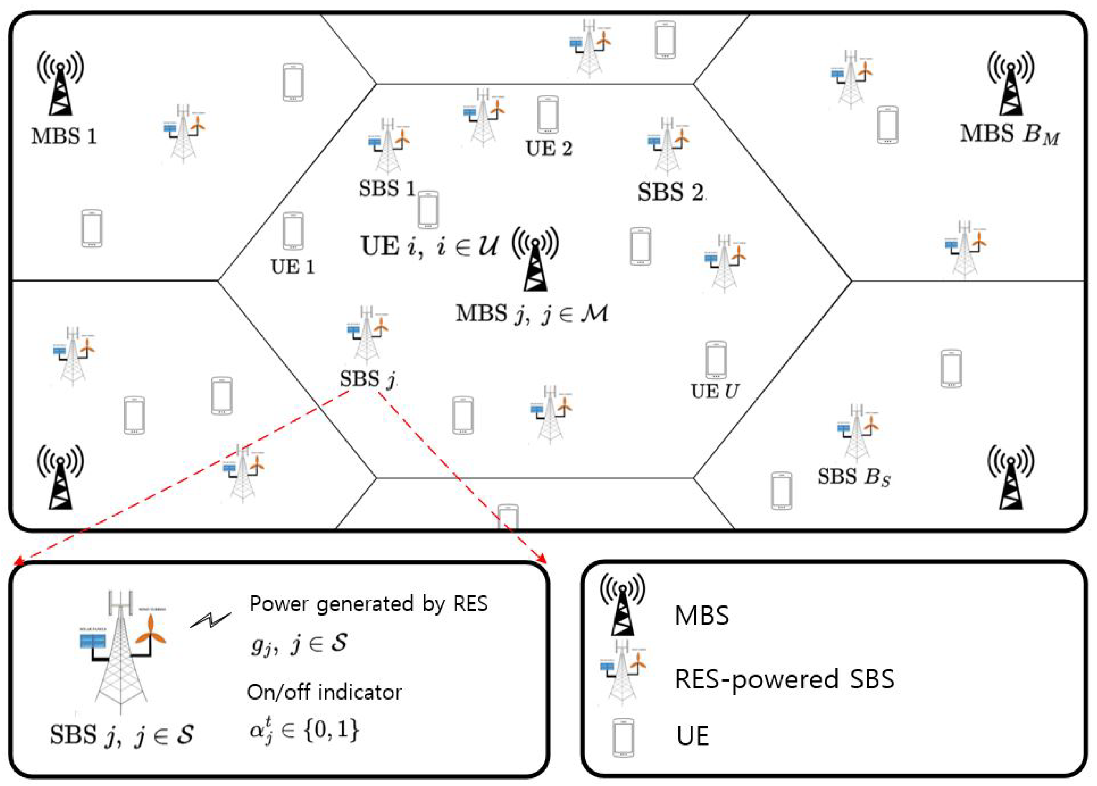
We further assume that each SBS has its own renewable energy source (RES). As a result, SBSs generate power to compensate their power consumption. The average power generated by the RES of each SBS over a long duration is denoted as . Note that we only consider the average power generation of the RES since we aim to achieve carbon neutrality in a long term. The overall network deployment is shown in Figure 1.
We assume that an UE is served by a single MBS or SBS, which provides the largest received signal power. Then, the rest of the MBSs/SBSs act as interference sources. As a result, when the received signal power of BS j is the strongest for UE i, the signal-to-interference-and-noise ratio (SINR) of a specific UE i at time slot t served by BS j can be calculated as
where is the channel gain between BS j and UE i and is thermal noise. Assuming round-robin scheduling, UE i’s achievable rate at time slot t is given by
where W is the bandwidth and is the number of pieces of UE being served by BS j.
2.2. Power Consumption Model
There are three components in the power consumption of BS j: (1) amplifier power , (2) maintenance power , and (3) switching power . Amplifier power is the power consumed by an amplifier, which is given by [25]
where is the power amplifier efficiency. Transmission power can range from 0 W to a specific maximum value, such as 40 W for an MBS and 0.5 W for an SBS. BSs also consume maintenance power even when the transmission power is nearly zero. This is caused by power supply, air conditioning, etc. We assume that the maintenance power has one of two fixed values; when the BS is on and when the BS is off. Thus, can be written as
Switching power is consumed when the BS is turned on or off. We assume that a fixed switching power is consumed. Then, is given by
Since the SBSs have their own RESs, a portion of the consumed power can be compensated. Therefore, we define power cost as
We aim to make the power cost around zero, i.e., to achieve a carbon-neutral system.
3. Objective Function
The aim of this paper is to maximize the net achievable rate while guaranteeing carbon neutrality. To do this, we adjust the transmission power of each SBS and even turn off some underutilized SBSs. However, there is a trade-off between maximizing the achievable rate and achieving carbon neutrality. This is because, when we set the overall SBS transmission powers high, this would increase the SBS coverage and, therefore, offload many pieces of UE to the SBS, which is beneficial to increase the achievable rate. On the other hand, this would obviously increase the power consumption and may not be good for carbon neutrality. Therefore, we need to carefully define our objective function to overcome such a trade-off. First, we consider the following objective function:
where is a design parameter that determines the trade-off between the achievable rate and the power consumption and is the maximum available power of BS j. However the result of solving objective function P1 is expected to be too sensitive to the selection of . If is large, the solution of P1 will tend to lower the power cost more than necessary. As a result, the underutilized power may cause a low achievable rate. On the other hand, if is small, it is more likely that the solution of P1 will fail to achieve carbon neutrality because the penalty of using high power is small. In short, an operator needs to find a proper to overcome the trade-off, which is not trivial. Therefore, we present another objective function P2, which is relatively insensitive to the selection of :
where is replaced by . The intuition for adding max operation is as follows. When is small, there will be no big difference in solving the objective function P1. However, when is large, the resulting power cost of P2 will also tend to be low, but not smaller than zero, because of the max operation. As a result, if the selection of is not too small, the solution of P2 will lead to the maximum use of available power, while is nearly zero, which is desirable in our case.
4. Implementation of the DDPG Algorithm
The objective function P2 is a mixed-integer nonlinear programming problem. To solve this, one needs to consider a huge amount of decision combinations, which may be prohibitive to finding the optimal solution. Even worse, the objective function must be solved every single time step. Therefore, rather than trying to solve P1 or P2, our approach is to use deep reinforcement learning, and the problem can be seen as an online decision problem. Since the transmission power of the SBS is continuous, we need a reinforcement learning algorithm that can handle continuous state/action spaces. Policy gradient algorithms are suitable for this case. The deterministic policy gradient (DPG) [26] algorithm is one of the policy gradient algorithms that can reduce the amount of computation dramatically compared to the basic stochastic policy gradient algorithm. However, the DPG can suffer from the overfitting problem when consecutive samples in the training process are highly correlated. Unlike the DPG, the DDPG can overcome the overfitting problem. The detailed explanation of the DDPG algorithm is provided in the following subsection.
4.1. Preliminaries
The DDPG algorithm mainly consists of two neural networks (NNs), actor and critic. In addition, there are two target NNs for actor and critic respectively, which helps stabilize the training process. The actor decides the action given the state, while the critic estimates the long-term reward of the state–action pair. In the DDPG, the NNs of the actor, the target actor, the critic, and the target critic are parameterized by , , , and , respectively. In the training phase, at each time slot, the system chooses an action according to , where is the output of the actor network given state and is the exploration noise a following normal distribution with standard deviation . The output of the actor network is deterministic, which is one of the advantages of the DDPG compared to traditional stochastic policy gradient methods [27]. The system then observes the reward and the state of the next time slot and repeats the sequence every time slot. During the sequence, the pair of is stored in the buffer, called the experience replay buffer. To improve the target actor network and the target critic network each step, a number of pairs are selected from the experience replay buffer with a given size , called the mini batch. By this procedure, the correlation of selected samples can be removed. Denoting the element of the mini batch as , the loss function used to optimize the critic is
where is a discount factor and is the output of the critic network given the state and action. The actor is also optimized with the following loss function:
Then, the original actor/critic network and the target actor/critic network have a specific weight added as
4.2. Problem Formulation
To implement the DDPG algorithm, we first need to define the state, action, and reward:
- State: Since the cellular network is operated in real-time, the proposed DDPG algorithm should operate as fast as possible. To this end, we define the state to be effective and simple. The state of our DDPG algorithm is given bywhere is the ratio of the pieces of UE served by BS j. The amount of information given by the state may look short and would not lead to good actions. However, the change of state not only gives the change of the UE served by certain BSs, but also some information of the UE locations. This is because the state change means a certain UE is handed off and might be on the edge of two BSs.
- Action: As explained in Section 3, we adjust the SBS transmission power and on/off switching for our goal. Therefore, the action is defined as follows:where is the output of the actor network. In the DDPG algorithm, the output of actor network is given by a continuous value. However, we need a discrete value to adjust SBS on/off switching. Thus, we convert the output vector as follows: (1) the action related to SBS power remains continuous since the power can be set as continuous; (2) we discretize the on/off-related components in (5)–(7) as if and if .
- Reward: Obviously, the reward is directly given by the objective function. Thus, the reward is defined as
4.3. Operation of DDPG Algorithm for Carbon Neutrality
The DDPG algorithm was directly implemented in the environment described in Section 2. Initially, all pieces of UE considered are randomly placed in the designated area. Then, as the pieces of UE move, the current state is examined by the BSs at each time slot. Because the state only needs the number of pieces of UE connected to the BSs, a central DDPG training server (may be located at the core network) can easily gather the required information. Once gathered, the server calculates the action quickly and only needs to send the information to the BSs, and not to the UE. After the BSs set their transmission power and on/off switching according to the actions delivered from the DDPG training server, the pieces of UE experience the network environment and report their channel status, which makes the BSs estimate the achievable rate of each user. The BSs can also recognize how many pieces of UE are served by certain cells. As a result, the state of the new time slot and the reward value can be fed to the DDPG training server. This allows the server to save the pair to the experience replay buffer. This process repeats, and when the experience replay buffer is sufficiently filled, the server starts updating the actor and critic parameters.
5. Simulation Results and Discussion
We evaluated the performance of the proposed DDPG algorithm through system-level simulation. To validate the benefits of our proposed scheme, we compared the proposed DDPG algorithm with (1) Q-learning —the Q-learning algorithm where the state is also discretized for the discrete operation nature of Q-learning; and (2) exact carbon neutral—a heuristic algorithm where SBSs have equal transmission power with exact carbon neutrality (i.e., the sum of the total power consumption is exactly the same as the power generated by RESs).
The simulation scenario contains 7 MBSs and 42 SBSs. the MBSs are located in a one-tier hexagonal model with an inter-site distance of 500 m. Six SBSs are equally deployed in each MBS coverage area. Forty pieces of UE are located inside each macrocell and randomly walk, where the speed is uniformly distributed in the range from 1 m/s to 10 m/s. Once the UE hits the edge of its MBS coverage, it bounces towards any direction that does not leave the original coverage. The transmission power of the MBS is set to 40 W, and the SBS is set to a maximum of 0.5 W. Path loss is modeled as a path-loss-exponent model with a parameter of 4. Both the actor network and the critic network consist of two hidden layers. In the actor network, each hidden layer has 128/64 neurons. For the critic network, both hidden layers have 64 neurons. All the activation functions are ReLU functions, except the last one of the actor network, which uses the hyperbolic tangent function. Note that the hyperbolic tangent function gives output in the range −1 to 1, so that it can be discretized into two levels with threshold 0. The learning rates of the actor network and the critic network are 0.0005, 0.001, respectively. The discount factor is 0.99. The standard deviation for the action exploration is 0.1. The size of the experience replay buffer is 50,000 with a mini batch size of 32. All the network parameters and hyperparameters are summarized in Table 1.
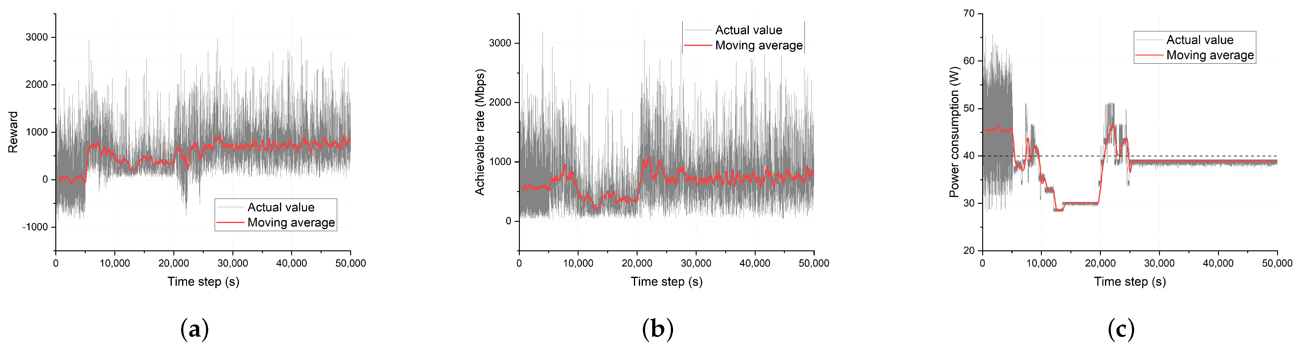
We first demonstrate the convergence of the sample case of the proposed DDPG algorithm with objective function P2 in Figure 3. After filling the experience replay buffer without training 5000 time steps, the rest of the training sequence is conducted for 45,000 time steps, which gives a total 50,000 time steps. Here, the time step was set to 1 s, which is long enough to cover the computational time of each time step, but not too long considering the UE location change due to mobility. The average power generation of the RES is 40 W. In all subfigures, we observe that in the early part of the time steps, there is no improvement since the DDPG algorithm only fills the experience buffer without training. After some training, the results converge with a small oscillation. Such an oscillation is natural in our case because the moving UE keeps changing the cellular environment. The most notable result is shown in Figure 3c. After some time steps, the power consumption converges very near the RES-generated power. This is clearly intended by the objective function P2. When the power consumption converges, the achievable rate and the reward also converge. The results show that the DDPG algorithm needs around 25,000 time slots to converge, which can be interpreted as the computational complexity of the DDPG algorithm [28]. This may seem large, but this process is only needed in the early stages of the training. In other words, the actions given by the DDPG algorithm stabilize afterwards.
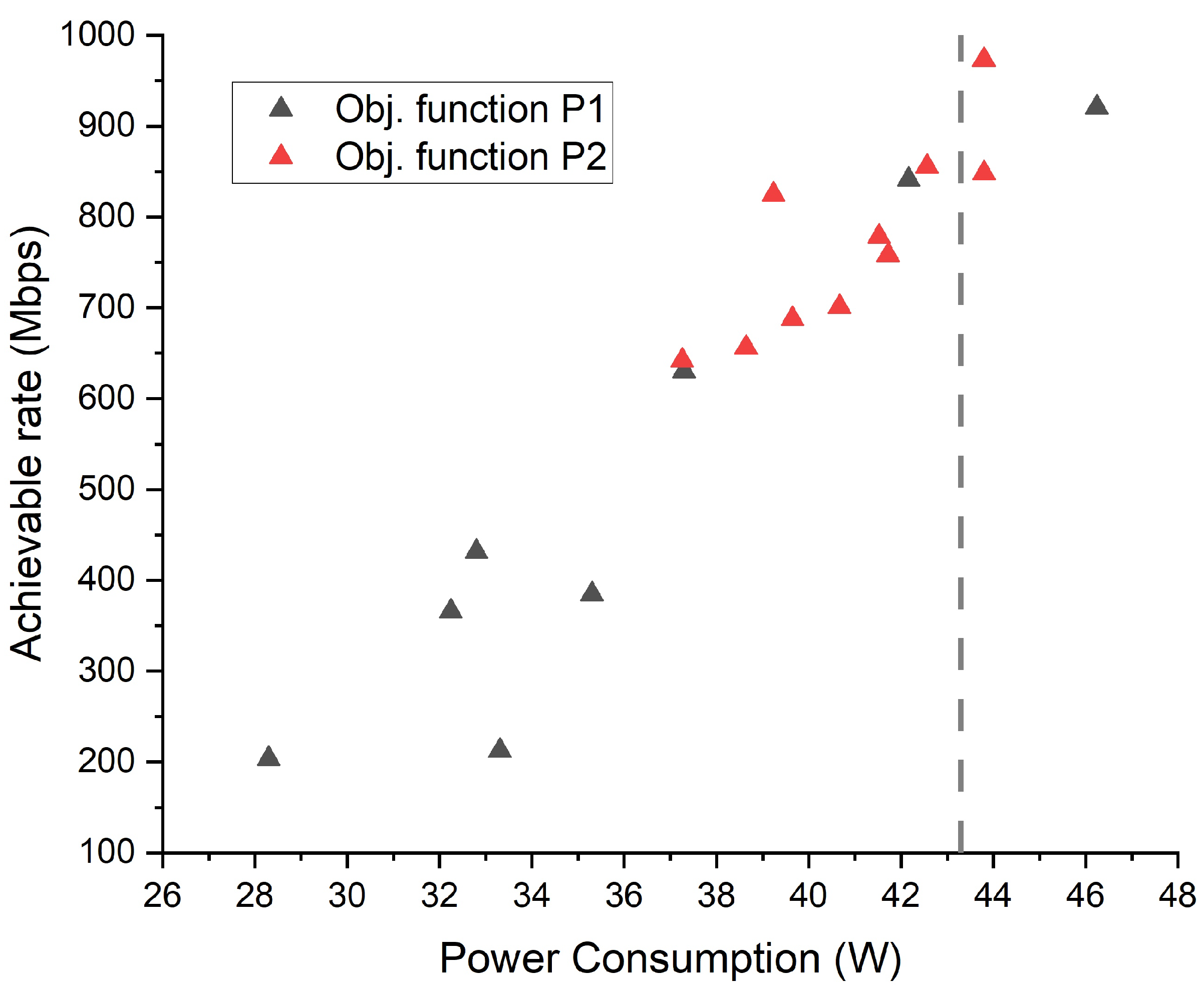
Figure 4 compares and shows the benefit of objective function P2. The sum of the average renewable power generation of the SBSs was set to 43.3 W. Each point is plotted for each value of for both objective functions by the proposed DDPG algorithm. was chosen from 0.1 to 1 with a 0.1 spacing. As shown in the figure, the points of objective function P2 are much more concentrated near the desired power consumption (i.e., the average renewable power generation) represented by the vertical dashed line. Specifically, the power cost and the achievable rate span from 28.30 W to 46.24 W and from 212.32 Mbps to 920.64 Mbps for objective function P1, while for objective function P2, they span from 37.26 W to 43.80 W and from 641.97 Mbps to 973.35 Mbps. The span range of objective function P1 is 2.74, 2.16-times larger than that of objective function P2. As expected, this implies that objective function P2 is much less sensitive to the choice of . Thus, one can more easily select , which could achieve carbon neutrality. Therefore, we only derive the results with objective function P2 afterwards.
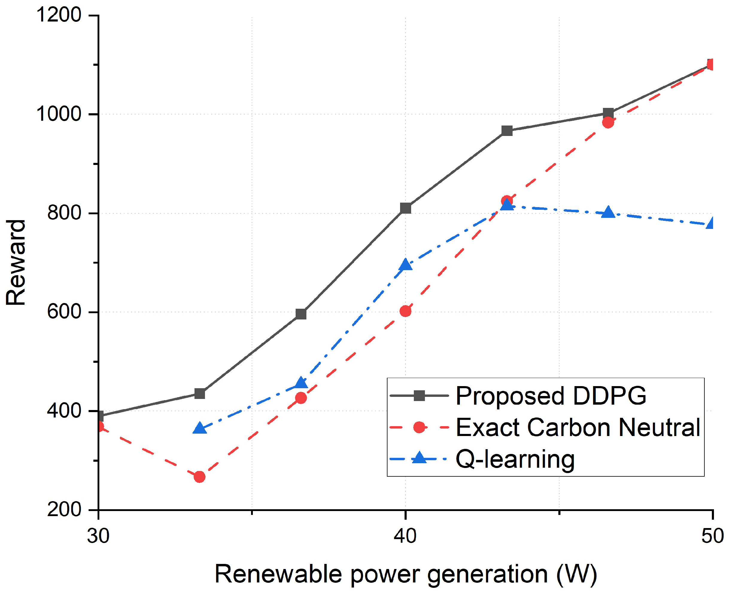
In Figure 5, we show the reward of each algorithm with several RES power generation values. The reward is estimated after 50,000 time slots of training. The DDPG model starts training when the experience replay buffer has 5000 data sets, i.e., after 5000 time slots. The proposed DDPG algorithm outperforms the Q-learning algorithm in all values of RES power generation. This is because Q-learning suffers from discretization upon selecting the action, specifically the SBS transmission power compared to continuous adjustment of SBS transmission power in the proposed DDPG algorithm. Furthermore, when the renewable power generation is higher than 46.6 W, Q-learning struggles more to find the appropriate combination of SBS transmission power and SBS on/off selection. Even worse, when there is a renewable power generation of 30 W, Q-learning even fails to reach carbon neutrality. As a result, the data point is omitted. In fact, if the level of discretization of Q-learning is denser, we can expect that the performance of the Q-learning algorithm might be closer to the performance of the DDPG algorithm. However, this will require a much higher computational complexity, which is not desirable for a real-time network. The heuristic algorithm showed similar results in some cases. In these cases, the resulting SBS transmission power was nearly the same as the SBS transmission power set by the DDPG algorithm, and all the SBSs were turned on in both algorithms. Nevertheless, the DDPG algorithm shows better performance overall. Specifically, the biggest gain of utilizing the proposed DDPG algorithm over the heuristic algorithm is 63%.
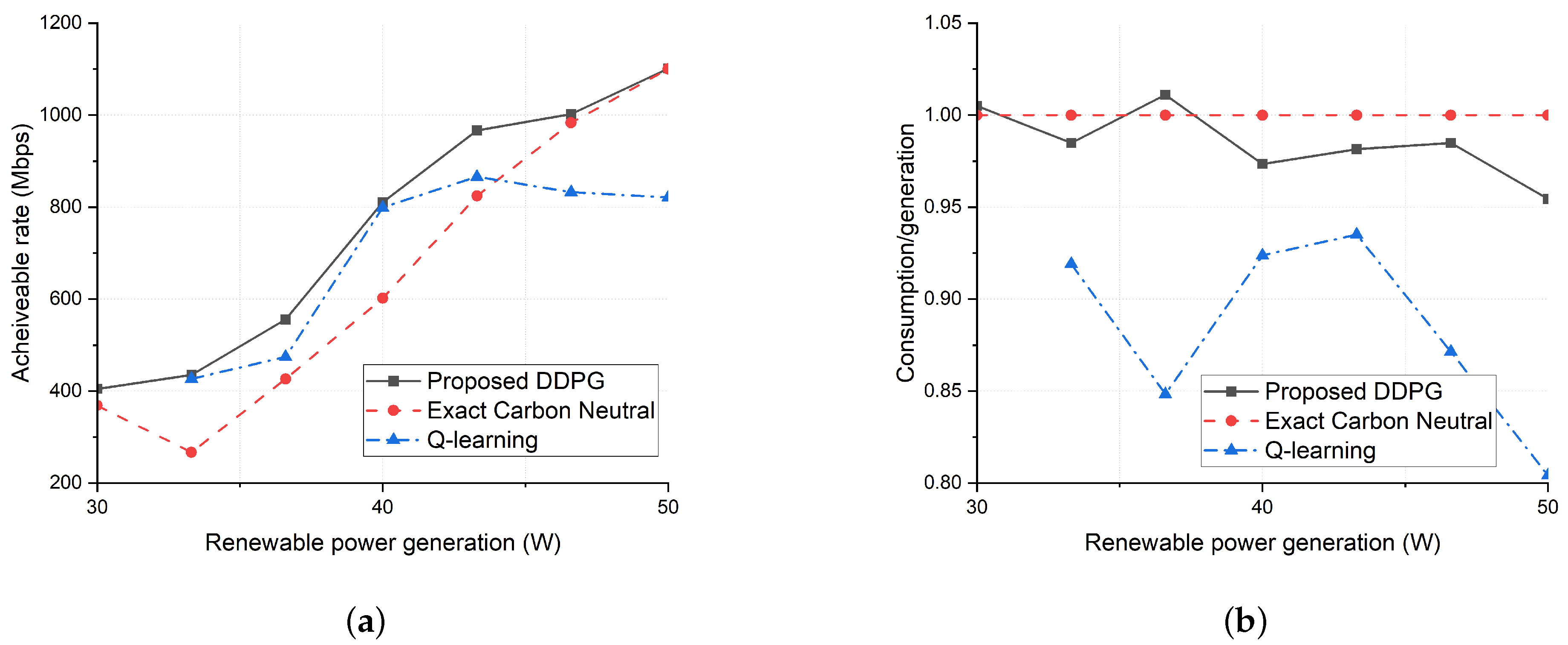
Figure 6 shows (a) the achievable rate and (b) the ratio of the consumed power to the average generated power. Note that the ratio is encouraged to be less than one to reach carbon neutrality. However, if the ratio is smaller than one, the network may be underutilizing the available amount of power and would result in a low achievable rate. In Figure 6a, the achievable rate shows a similar pattern to the reward in Figure 5. This implies that the low achievable rate caused the low reward value of Q-learning compared to the DDPG algorithm. Furthermore, the difference of the achievable rate between the DDPG algorithm and Q-learning matches the ratio in Figure 6b. As expected, it is shown that the low achievable rate is caused by low utilization of the available power. The heuristic algorithm manages to achieve carbon neutrality perfectly, but the achievable rate is always lower than the DDPG algorithm because the transmission power was simply set equal. This means that adjusting the SBS transmission power based on the environment is crucial for increasing the achievable rate.
6. Conclusions
We proposed a DDPG algorithm to achieve the carbon neutrality of a UDN. In addition, we aimed to obtain the highest achievable rate possible with the given power constraints. The algorithm adjusted the transmission power and BS on/off decision to balance the power consumption with power generation by RESs. We also designed the reward function of the DDPG algorithm to achieve carbon neutrality smoothly. The state of the DDPG algorithm was set to be simple, but effective to be operated in a real-time network. We conducted an extensive system-level simulation to validate the performance of our DDPG algorithm. We compared the DDPG algorithm with a heuristic algorithm and the Q-learning method as a baseline. It was shown that our simple, but effective DDPG algorithm is able to achieve carbon neutrality and a better achievable rate compared to the baseline schemes. To be specific, the reward value of the proposed DDPG algorithm was up to 63% higher that the baseline schemes.
Finally, it would be interesting to investigate the optimality gap of the proposed method, for example using commercial optimization solvers such as GAMS. However, that would be very computationally challenging, and investigating the optimality gap remains as future work.
Author Contributions
Conceptualization, H.K. (Hojin Kim), J.S. and H.K. (Hongseok Kim); methodology, H.K. (Hojin Kim) and H.K. (Hongseok Kim); software, H.K. (Hojin Kim); validation, H.K. (Hojin Kim), J.S. and H.K. (Hongseok Kim); writing—original draft preparation, H.K. (Hojin Kim), J.S. and H.K. (Hongseok Kim); writing—review and editing, H.K. (Hojin Kim), J.S. and H.K. (Hongseok Kim); visualization, H.K. (Hojin Kim); supervision, J.S. and H.K. (Hongseok Kim). All authors have read and agreed to the published version of the manuscript.
Funding
This work was supported by the National Research Foundation (NRF), Korea, under project BK21 FOUR and the National Research Foundation of Korea (NRF) grant funded by the Korea government (MSIT) (NRF-2021R1A2C1095435).
Institutional Review Board Statement
Not applicable.
Informed Consent Statement
Not applicable.
Conflicts of Interest
The authors declare no conflict of interest.
Abbreviations
The following abbreviations are used in this manuscript:
| DDPG | Deep deterministic policy gradient |
| DPG | Deterministic policy gradient |
| UDN | Ultra-dense network |
| BS | Base station |
| MBS | Macro base station |
| SBS | Small base station |
| UE | User equipment |
| RES | Renewable energy source |
| DRL | Deep reinforcement learning |
| DQN | Deep Q network |
| SINR | Signal-to-interference-and-noise ratio |
| NN | Neural network |
References
- Ge, X.; Tu, S.; Mao, G.; Wang, C.X.; Han, T. 5G ultra-dense cellular networks. IEEE Wirel. Commun. 2016, 23, 72–79. [Google Scholar] [CrossRef] [Green Version]
- Malmodin, J.; Lundén, D. The energy and carbon footprint of the global ICT and E&M sectors 2010–2015. Sustainability 2018, 10, 3027. [Google Scholar]
- Roll out 5G without Increasing Energy Consumption. Available online: https://www.ericsson.com/en/about-us/sustainability-and-corporate-responsibility/environment/product-energy-performance (accessed on 13 May 2022).
- Moon, S.; Kim, H.; Yi, Y. BRUTE: Energy-efficient user association in cellular networks from population game perspective. IEEE Trans. Wirel. Commun. 2015, 15, 663–675. [Google Scholar] [CrossRef]
- Lee, G.; Kim, H. Green small cell operation using belief propagation in wireless networks. In Proceedings of the 2014 IEEE Globecom Workshops (GC Wkshps), Austin, TX, USA, 8–12 December 2014; pp. 1266–1271. [Google Scholar]
- Jeong, J.; Kim, H. On Optimal Cell Flashing for Reducing Delay and Saving Energy in Wireless Networks. Energies 2016, 9, 768. [Google Scholar] [CrossRef] [Green Version]
- Choi, Y.; Kim, H. Optimal scheduling of energy storage system for self-sustainable base station operation considering battery wear-out cost. Energies 2016, 9, 462. [Google Scholar] [CrossRef] [Green Version]
- Liu, C.; Natarajan, B.; Xia, H. Small cell base station sleep strategies for energy efficiency. IEEE Trans. Veh. Technol. 2015, 65, 1652–1661. [Google Scholar] [CrossRef]
- Oh, E.; Son, K. A unified base station switching framework considering both uplink and downlink traffic. IEEE Wirel. Commun. Lett. 2016, 6, 30–33. [Google Scholar] [CrossRef]
- Son, K.; Kim, H.; Yi, Y.; Krishnamachari, B. Base station operation and user association mechanisms for energy-delay tradeoffs in green cellular networks. IEEE J. Sel. Areas Commun. 2011, 29, 1525–1536. [Google Scholar] [CrossRef]
- Feng, M.; Mao, S.; Jiang, T. BOOST: Base station on-off switching strategy for energy efficient massive MIMO HetNets. In Proceedings of the IEEE INFOCOM 2016—The 35th Annual IEEE International Conference on Computer Communications, San Francisco, CA, USA, 10–15 April 2016; pp. 1–9. [Google Scholar]
- Peng, C.; Lee, S.B.; Lu, S.; Luo, H. GreenBSN: Enabling energy-proportional cellular base station networks. IEEE Trans. Mob. Comput. 2014, 13, 2537–2551. [Google Scholar] [CrossRef]
- Celebi, H.; Yapıcı, Y.; Güvenç, I.; Schulzrinne, H. Load-based on/off scheduling for energy-efficient delay-tolerant 5g networks. IEEE Trans. Green Commun. Netw. 2019, 3, 955–970. [Google Scholar] [CrossRef] [Green Version]
- Salem, F.E.; Altman, Z.; Gati, A.; Chahed, T.; Altman, E. Reinforcement learning approach for advanced sleep modes management in 5G networks. In Proceedings of the 2018 IEEE 88th Vehicular Technology Conference (VTC-Fall), Chicago, IL, USA, 27–30 August 2018; pp. 1–5. [Google Scholar]
- El-Amine, A.; Hassan, H.A.H.; Iturralde, M.; Nuaymi, L. Location-Aware sleep strategy for Energy-Delay tradeoffs in 5G with reinforcement learning. In Proceedings of the 2019 IEEE 30th Annual International Symposium on Personal, Indoor and Mobile Radio Communications (PIMRC), Istanbul, Turkey, 8–11 September 2019; pp. 1–6. [Google Scholar]
- Pujol-Roigl, J.S.; Wu, S.; Wang, Y.; Choi, M.; Park, I. Deep reinforcement learning for cell on/off energy saving on wireless networks. In Proceedings of the 2021 IEEE Global Communications Conference (GLOBECOM), Madrid, Spain, 7–11 December 2021; pp. 1–7. [Google Scholar]
- Ye, J.; Zhang, Y.J.A. DRAG: Deep reinforcement learning based base station activation in heterogeneous networks. IEEE Trans. Mob. Comput. 2019, 19, 2076–2087. [Google Scholar] [CrossRef] [Green Version]
- Giannopoulos, A.; Spantideas, S.; Kapsalis, N.; Karkazis, P.; Trakadas, P. Deep reinforcement learning for energy-efficient multi-channel transmissions in 5G cognitive hetnets: Centralized, decentralized and transfer learning based solutions. IEEE Access 2021, 9, 129358–129374. [Google Scholar] [CrossRef]
- Iqbal, A.; Tham, M.L.; Chang, Y.C. Double deep Q-network-based energy-efficient resource allocation in cloud radio access network. IEEE Access 2021, 9, 20440–20449. [Google Scholar] [CrossRef]
- Kim, E.; Jung, B.C.; Park, C.Y.; Lee, H. Joint Optimization of Energy Efficiency and User Outage Using Multi-Agent Reinforcement Learning in Ultra-Dense Small Cell Networks. Electronics 2022, 11, 599. [Google Scholar] [CrossRef]
- Kim, S.; Son, J.; Shim, B. Energy-Efficient Ultra-Dense Network Using LSTM-based Deep Neural Networks. IEEE Trans. Wirel. Commun. 2021, 20, 4702–4715. [Google Scholar] [CrossRef]
- Lillicrap, T.P.; Hunt, J.J.; Pritzel, A.; Heess, N.; Erez, T.; Tassa, Y.; Silver, D.; Wierstra, D. Continuous control with deep reinforcement learning. arXiv 2015, arXiv:1509.02971. [Google Scholar]
- Qiu, C.; Hu, Y.; Chen, Y.; Zeng, B. Deep deterministic policy gradient (DDPG)-based energy harvesting wireless communications. IEEE Internet Things J. 2019, 6, 8577–8588. [Google Scholar] [CrossRef]
- Lu, Y.; Lu, H.; Cao, L.; Wu, F.; Zhu, D. Learning deterministic policy with target for power control in wireless networks. In Proceedings of the 2018 IEEE Global Communications Conference (GLOBECOM), Abu Dhabi, United Arab Emirates, 9–13 December 2018; pp. 1–7. [Google Scholar]
- Auer, G.; Giannini, V.; Desset, C.; Godor, I.; Skillermark, P.; Olsson, M.; Imran, M.A.; Sabella, D.; Gonzalez, M.J.; Blume, O.; et al. How much energy is needed to run a wireless network? IEEE Wirel. Commun. 2011, 18, 40–49. [Google Scholar] [CrossRef]
- Silver, D.; Lever, G.; Heess, N.; Degris, T.; Wierstra, D.; Riedmiller, M. Deterministic policy gradient algorithms. In Proceedings of the 31st International Conference on Machine Learning, Beijing, China, 21–26 June 2014; pp. 387–395. [Google Scholar]
- Thrun, S.; Littman, M.L. Reinforcement Learning: An Introduction; MIT Press: Cambridge, MA, USA, 2018. [Google Scholar]
- Yu, L.; Xie, W.; Xie, D.; Zou, Y.; Zhang, D.; Sun, Z.; Zhang, L.; Zhang, Y.; Jiang, T. Deep reinforcement learning for smart home energy management. IEEE Internet Things J. 2019, 7, 2751–2762. [Google Scholar] [CrossRef] [Green Version]
Figure 1.
Network deployment with RES-powered SBSs.

Figure 2.
Illustration of the DDPG algorithm.

Figure 3.
Convergence of the DDPG algorithm. In each subfigure, actual values are shown as grey lines, and red lines represent the moving average of the actual value with a window size 500. (a) Reward, (b) achievable rate, and (c) power consumption.
Figure 3.
Convergence of the DDPG algorithm. In each subfigure, actual values are shown as grey lines, and red lines represent the moving average of the actual value with a window size 500. (a) Reward, (b) achievable rate, and (c) power consumption.

Figure 4.
Achievable rate and power consumption with for different objective functions. The vertical dashed line () represents the average power generated by the RES.
Figure 4.
Achievable rate and power consumption with for different objective functions. The vertical dashed line () represents the average power generated by the RES.

Figure 5.
Reward values after training of the DDPG algorithm.

Figure 6.
Comparison of performances among different schemes after training. (a) Achievable rate and (b) ratio of power consumed to power generated by RESs.
Figure 6.
Comparison of performances among different schemes after training. (a) Achievable rate and (b) ratio of power consumed to power generated by RESs.


Table 1.
Simulation parameters.
| Network Parameter | Value | Hyperparameter | Value |
|---|---|---|---|
| Simulation count | 50,000 | Learning rate | Actor: 0.0005/ Critic: 0.001 |
| Time step | 1 s | Discount factor | 0.99 |
| Carrier frequency | 2 GHz | Mini batch size | 32 |
| System bandwidth | 20 MHz | Size of experience replay buffer | 50,000 |
| MBS deployment | 1 tier hexagonal | Soft update weight | 0.05 |
| SBS deployment | 6 per MBS | Exploration standard dev. | 0.1 |
| Max transmission power | MBS: 40 W/SBS: 0.5 W | ||
| UE deployment | 40 | ||
| Mobility | uniform in range [1–10] m/s | ||
| Path loss exponent | 4 | ||
| Antenna pattern | Omnidirectional | ||
| Maintenance p. (ON) | 6.8 W | ||
| Amplifier efficiency | 0.25 | ||
| Maintenance p. (OFF) | 4.3 W |
Publisher’s Note: MDPI stays neutral with regard to jurisdictional claims in published maps and institutional affiliations. |
© 2022 by the authors. Licensee MDPI, Basel, Switzerland. This article is an open access article distributed under the terms and conditions of the Creative Commons Attribution (CC BY) license (https://creativecommons.org/licenses/by/4.0/).
Share and Cite
MDPI and ACS Style
Kim, H.; So, J.; Kim, H. Carbon-Neutral Cellular Network Operation Based on Deep Reinforcement Learning. Energies 2022, 15, 4504. https://0-doi-org.brum.beds.ac.uk/10.3390/en15124504
AMA Style
Kim H, So J, Kim H. Carbon-Neutral Cellular Network Operation Based on Deep Reinforcement Learning. Energies. 2022; 15(12):4504. https://0-doi-org.brum.beds.ac.uk/10.3390/en15124504
Chicago/Turabian StyleKim, Hojin, Jaewoo So, and Hongseok Kim. 2022. "Carbon-Neutral Cellular Network Operation Based on Deep Reinforcement Learning" Energies 15, no. 12: 4504. https://0-doi-org.brum.beds.ac.uk/10.3390/en15124504
Note that from the first issue of 2016, this journal uses article numbers instead of page numbers. See further details here.