Smart Energy Management: A Comparative Study of Energy Consumption Forecasting Algorithms for an Experimental Open-Pit Mine

Abstract

The mining industry’s increased energy consumption has resulted in a slew of climate-related effects on the environment, many of which have direct implications for humanity’s survival. The forecast of mine site energy use is one of the low-cost approaches for energy conservation. Accurate predictions do indeed assist us in better understanding the source of high energy consumption and aid in making early decisions by setting expectations. Machine Learning (ML) methods are known to be the best approach for achieving desired results in prediction tasks in this area. As a result, machine learning has been used in several research involving energy predictions in operational and residential buildings. Only few research, however, has investigated the feasibility of machine learning algorithms for predicting energy use in open-pit mines. To close this gap, this work provides an application of machine learning algorithms in the RapidMiner tool for predicting energy consumption time series using real-time data obtained from a smart grid placed in an experimental open-pit mine. This study compares the performance of four machine learning (ML) algorithms for predicting daily energy consumption: Artificial Neural Network (ANN), Support Vector Machine (SVM), Decision Tree (DT), and Random Forest (RF). The models were trained, tested, and then evaluated. In order to assess the models’ performance four metrics were used in this study, namely correlation (R), mean absolute error (MAE), root mean squared error (RMSE), and root relative squared error (RRSE). The performance of the models reveals RF to be the most effective predictive model for energy forecasting in similar cases.

1. Introduction

Global energy demand has been continuously rising since the turn of the century, owing to rising social demands and a wide range of economic operations, including mining industry [1,2]. Open-pit mining, strip mining, quarrying, and underground excavation are all methods of locating, extracting, beneficiating, and processing solid minerals from the earth’s crust. For thousands of years, mining has been an important aspect of human activity, providing raw materials for enhancing security and quality of life and establishing the modern industrial society. Surface mines, which range from large-scale coal open-pit mines to small mineral or rock quarries, account for the majority of the mining operations [3,4]. Despite society’s increased efforts in recycling and dematerialization, mining activity is developing globally due to rapid urbanization, which creates a need for more metals and minerals in structures and all sorts of consumer products. Another reason for this expansion is that the richest ores have long been depleted, therefore more rock ore excavation is required to extract the same amount of pure mineral, resulting in a substantial rise in energy consumption [5,6]. The entire quantity of energy consumed in the mining and minerals industry is estimated to be 4–7% of worldwide energy production [7]. As a result, to rationalize energy use in open-pit mines, a strong energy management system is required.

The ISO 50001 is a standard that was published in July 2011 to guide the adoption of an Energy Management System (EnMS). The standard is expected to have a 60 percent impact on global energy use due to its broad applicability across national economic sectors.

According to certain case studies, putting the ISO 50001 standard in place increased energy performance indicators. Competitors will be even more motivated to adopt the standard because of these positive results [8].

The major goal of the ISO 50001 Energy Management System standard is to enable enterprises to become more energy efficient. However, the integration of energy management into the industrial decision-making process has received little attention. As a result, it is critical to investigate the domain of energy management in order to assist industrial decision-makers in identifying the specific actions required to reduce energy management lags [9].

In the context of energy management and conservation, smart grid system maintenance and scheduling, and IoT data-driven energy consumption predictions are important study areas. For energy consumption pattern analytics, artificial intelligence (AI) technologies such as machine learning (ML) and integrated deep learning (DL) are becoming increasingly relevant [10].

In this study, we focus on establishing a smart energy management system for energy forecasting in the experimental open-pit mine of Benguerir, in order to facilitate the tracing and the supervision of the energy consumption for the different users. This work also provides a tool for energy prediction in the mining industry using RapidMiner. In this context, we compare the efficacy and accuracy of four machine learning (ML) algorithms, namely Artificial Neural Network (ANN), Support Vector Machine (SVM), Decision Tree (DT), and Random Forest (RF) using the data collected from a smart grid built in the experimental open-pit mine.

The main contributions of this study are summarized as follows:

(a)

This study presents one of the few studies made to forecast the energy consumption behavior in the mining industry and in particular the open-pit mines. It presents a comparison of some of the well-known ML techniques and evaluates their performance.

(b)

Four ML algorithms namely, Artificial Neural Network, Support Vector Machine, Random Forest, and Decision Tree were applied to a dataset acquired from an experimental open-pit mine. The different models were trained, tested, and then evaluated.

(c)

Four metrics were used to assess the models’ performance, namely correlation, root mean squared error, mean absolute error, and root relative squared error. After parameter tuning, Random Forest showed the best performance among all four algorithms.

(d)

Managers, technicians, and supervisors will be able to view real-time energy consumption, analyze future warnings based on the current condition of load consumption and make timely decisions.

The remainder of this work is arranged in the following manner. Section 2 examines the literature on time-series forecasting, machine learning, and existing assessments of energy consumption prediction methods. Section 3 discusses the methodology and materials utilized in this work to estimate energy use, as well as the energy consumption dataset, AI model parameters, and performance indicators. The diverse findings produced by each model are shown and discussed in Section 4. Finally, Section 5 draws conclusions and makes recommendations for future research on this topic.

2. Related Works

Numerous studies have been undertaken on time series forecasting, and many successful implementations and approaches have demonstrated the benefit in sectors such as power consumption forecasts [10,11,12,13,14,15,16,17,18,19,20,21]. Forecasting IoT energy usage is a prominent topic, and research into it using machine learning and deep learning methods has progressed quickly.

Biswas et al. [11] construct an ANN structure for residential power load forecasting, based on the fact that artificial neural networks (ANN) can simulate more volatile data. González-Briones et al. [13] looked at ANN, support vector machine (SVM), decision tree (DT), and rule-based systems as machine learning methods for energy consumption data predictions and mining. For the same problem, more novel solutions were proposed with DL. Marino et al. [14] suggested using LSTM neural networks to forecast household energy consumption. Kong et al. [15] used an LSTM model to anticipate domestic energy consumption with unpredicted human behaviors. Kim and Cho [16] use a convolutional neural network (CNN) and LSTM to estimate residential building energy consumption. While time series forecasting research becomes more difficult, more advanced DL architectures for time series data forecasting have been developed. In a study carried out by Binrong Wu et al. [17] a deep learning algorithm, namely, CNN, was employed to extract textual information from social media information automatically. For building energy consumption forecasts, Nivethitha Somu et al. [18] applied kCNN-LSTM, a deep learning framework, on the energy consumption data recorded at predefined intervals and evaluated its accuracy. In another study, Lianyi Liu and Lifeng Wu [19] proposed a new adjacent non-homogeneous grey model to predict renewable energy consumption in Europe. Deep reinforcement learning (DRL) techniques for building energy consumption analytics were investigated by Liu et al. [20]. They also used a multi-step forecasting method to improve on the single step forecasting method.

The majority of studies, as seen so far, tend to focus solely on the residential sector. This is due to the increased availability of data from the residential sector or households. While a study of the home sector can yield some helpful results, extrapolating them to the entire economy can be misleading [22]. In terms of the nature of demand shocks that might affect the pattern of power consumption, the industrial sector differs significantly from the residential sector [23]. Therefore, more research into the industrial sector is required.

In this context, there has not been much research on energy forecasting, particularly in the mining industry and more specifically in the open-pit mines. Oussama et al. [24] introduced a rapid forest quantile regression technique to forecast the energy demand response based on data from different historical scenarios in an experimental open-pit mine, which is one of the new extant studies in this field. Our work comes to investigate further the energy forecasting in the open-pit mine using four well-known ML techniques namely SVM, ANN, DT, and RF to facilitate the evaluation of the energy consumption and draw early expectations for energy use within the mining industry which helps significantly in the decision-making process.

In a study carried out by Oussama et al. [25], the authors present a summary of multiple studies made in the energy consumption forecasting in different applications as illustrated in

Table 1. Comparative study of energy consumption.

Team	Year	Application	Methodology	Reference
Solomon	2011	Large commercial building	SVM (RBF)	[26]
Edwards	2012	Residential building	ANN LS-SVM MLR	[27]
Dagnely	2015	Nonresidential building	OLS, SVM (RBF)	[28]
Massana	2015	Nonresidential building	MLR, ANN (MLP, SVM (PUK)	[29]
Penya	2011	Nonresidential building	Poly, Exponential, mixed, AR, ANN, SVM	[30]
Zhao	2010	Multiple buildings	SVM (RBF)	[31]
Paudel	2015	Building	SVM (RBF)	[32]
Jain	2014	Multifamily residential building	SVM (RBM)	[33]
Men	2014	Bioclimatic building	ANN (NARX)	[34]
Penya	2011	Air-conditioned nonresidential building	AR ARIMA, ANN, Bayesian Network	[35]
González	2005	Nonresidential building	ANN	[36]
Fernández	2011	Nonresidential building	AR, SVM (RBF), Poly, ANN	[37]
Escrivá	2011	Nonresidential building	ANN (MLP)	[38]
Kamaev	2012	Shopping center	ANN	[39]
Bagnasco	2012	Hospital facilities	ANN (BPNN)	[40]
Borges	2013	Multifamily residential building	SVM(RBF) AR	[41]
Lai	2008	Residential building	SVM	[42]
Farzana	2014	Residential building	ANN(BPNN)	[43]
Yuan	2018	University Campus	ANN	[44]
Yun	2020	Ships of green ports	ANN	[45]
Minglei	2020	Hotel	SVM	[46]

.

3. Materials and Methods

The following is a preliminary outline of the proposed method. Figure 1 show the flowchart of the followed methodology, as a first step in the procedure, the experimental open-pit mine’s acquired historical data are cleaned. After then, the main dataset is split into training, testing, and validation sets. The dataset is then subjected to four machine learning algorithms (SVM, ANN, DT, and RF) using the Rapid Miner tool. Four metrics, the correlation, absolute error, relative error, and mean square, are used to generate and evaluate the forecast. The parameter tuning process takes place during the whole procedure in order to generate the best performance of the four models. In the following subsections, we present the studied dataset and the utilized algorithms in this study.

3.1. Data Description

Figure 2 depicts the energy consumption behavior during 24 h, based on the data collected from the experimental open-pit mine.

The original energy consumption data were gathered from Benguerir’s experimental open-pit mine. Various measurements, including current, voltage, frequency, power, and power factor, were recorded and monitored. Every second, a new record is set. We gathered data from 21 sites at the experimental open-pit mine during 24 h, totaling 3,008,330 records. In this research, we focused on using data from a single site in the energy forecasting process, since the same procedure can be applied to the other sites following the same steps. After using a Python program to filter and clean the data, 26,395 records remained.

3.2. Support Vector Machine

3.2.1. Definition

SVM is a data mining algorithm that is often regarded as one of the most reliable and accurate among all data mining algorithms [47]. Due to its capacity to efficiently provide answers to non-linear issues in a variety of data sizes (Hai-Xiang [48], SVM is becoming more widely used in research). Support Vector Regression (SVR) is the SVM used for regression, and it has emerged as a prominent data-driven tool for forecasting building energy demand. The basic goal of SVR is to generate a decision function, F(xi), from past data, a process known as training. It is essential that the anticipated outcome for the given input xi does not differ from the true target yi by more than the predetermined threshold ε. This function is expected as follows

F(xi) = (ε, φ(xi)) + b (1))

(1)

It’s worth noting that SVM, and specifically SVR, are preferable to other models since their framework is easily adapted for a variety of problems and can produce optimal solutions all over the world [49].

The following Figure 3 describes the SVM algorithm process.

3.2.2. Support Vector Machine Parameters

RapidMiner documentation provides all the information about the different features and models within the software, this includes the models’ parameters. SVM has several parameters [50] namely:

• Kernel type: This parameter determines the type of kernel function to be used. The following kernel types can be used: multiquadric, dot, radial, polynomial, neural, anova, epachnenikov, gaussian combination.
• Kernel cache: It is an expert parameter. It determines the cache size in megabytes for kernel evaluations.
• C: This is the SVM complexity constant that determines the misclassification tolerance, with larger C values allowing for ‘softer’ bounds and lower values allowing for ‘harder’ limits. Over-fitting can occur when the complexity constant is too large, while over-generalization can occur when the complexity constant is too small. The Range is real.
• Convergence epsilon: This is an optimizer parameter. It specifies the precision of the KKT conditions.
• Max iterations: This is an optimizer parameter. It specifies to stop iterations after a specified number of iterations. Range: integer.

3.3. Artificial Neural Network

3.3.1. Definition

The artificial neural network (ANN) is a non-linear computing model that mimics the functional notions of the human brain [51]. ANN is a powerful tool for tackling nonlinear issues, and it works best with large datasets that provide enough data for the neural network to train the model [52]. As shown in Figure 4 below, the basic form of ANN consists of three layers: input, hidden, and output. The input layer is used to train the model, the hidden layer is a link between the input and output layers that can be changed depending on the kind of ANN, and the output layer is where the result is displayed [53]. Back Propagation Neural Networks (BPNN), Feed Forward Neural Networks (FFNN), Adaptive Network-based Fuzzy Inference System (ANFIS), and other forms of ANNs exist. The feed-forward method is the most widely used [54]. The illustrated diagram of feed-forward neural network architecture with two hidden layers are shown in Figure 3.

3.3.2. Artificial Neural Network Parameters

The main parameters for this model [55] are the following:

• Hidden layers: The name and size of all hidden levels are described by this parameter. This option allows the user to define the neural network’s structure. Each entry in the list describes a different hidden layer. The name and size of the concealed layer are required for each entry. The name of the layer can be chosen at will. It is simply used to show the model, the Range is real.
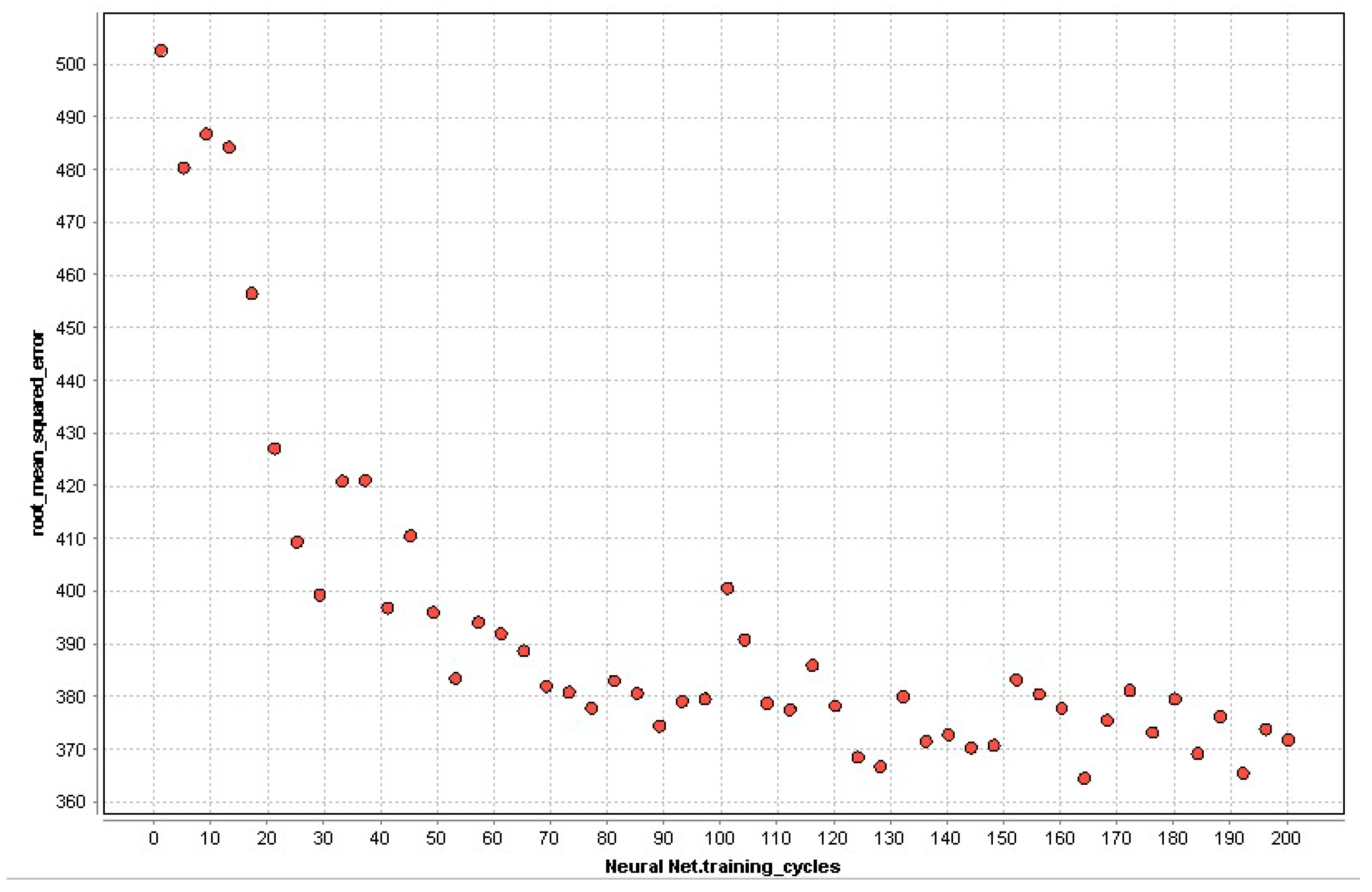
• Training cycles: The number of training cycles utilized to train the neural network is specified by this parameter. Back-propagation compares the output values to the correct solution in order to compute the value of a preset error function. The error is subsequently relayed to the rest of the network. The algorithm modifies the weights of each link based on this information in order to minimize the error function’s value by a tiny amount. This procedure is repeated an undetermined number of times n. This argument can be used to specify the number n. The Range is real.
• Learning rate: This parameter controls how much the weights are changed at each phase. It must not be zero. The Range is real.
• Momentum: The momentum merely adds a percentage of the previous weight update to the new one. Hence, local maxima are avoided, and optimization paths are smoothed. The Range is real.

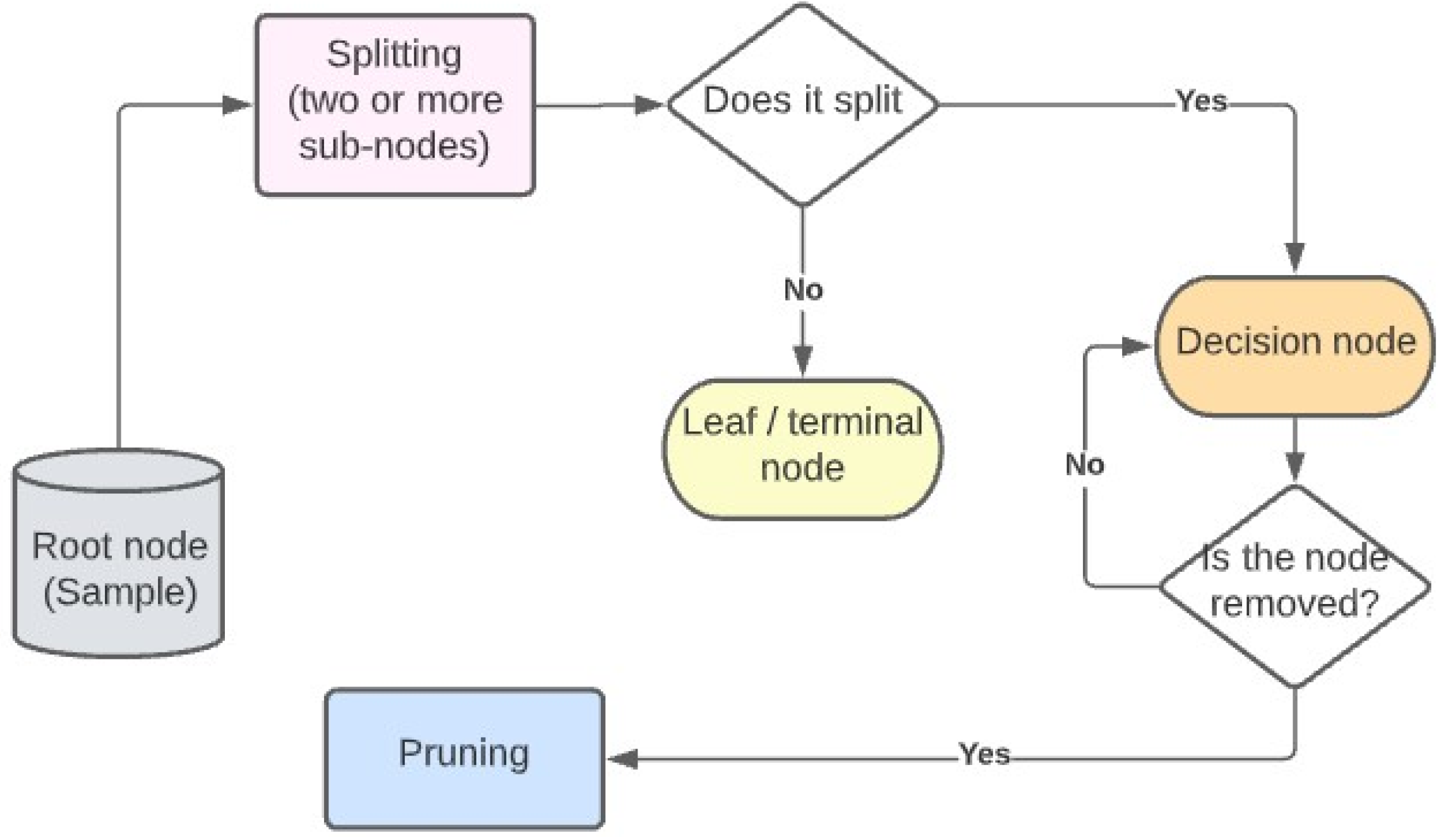
3.4. Decision Tree

3.4.1. Definition

The Decision Tree (DT) approach (Figure 5) divides data into categories by using a tree-like flowchart. Decision Trees are a flexible procedure that can learn from a larger amount of training data [56]. The DT is easier to understand than other data-driven methodologies, and its application does not necessitate significant calculation understanding. However, it frequently leads to significant deviations between predictions and actual results. DT is better suited to forecasting category characteristics than estimating numerical variables [57].

The Figure 6 depicts the Decision Tree process. The root node represents the sample being analyzed and is found at the top of a tree. Splitting is the process of dividing a node into sub-nodes; when a sub-node can be split into further nodes then it is called decision node. Leaf nodes are tree nodes that do not have any additional split nodes. Pruning is the process of removing sub-nodes from a decision node; it is the inverse of splitting, and it is intended to prevent over-fitting.

3.4.2. Decision Tree Parameters

In RapidMiner Decision Tree Documentation [58] we find multiple parameters such as:

• Criterion: Selects the criterion by which Attributes will be separated based on. The split value is optimized for each of these criteria in relation to the chosen criterion. Information gain, gain ratio, gini index, accuracy, and least square are some of its variables.
• Maximal depth: The size and properties of the ExampleSet determine the depth of the tree. This parameter is used to limit the decision tree’s depth. If it is set to ‘−1’, the maximal depth parameter has no effect on the tree’s depth. The tree is created in this situation until additional halting requirements are met. A tree with a single node is formed if its value is set to ‘1’.
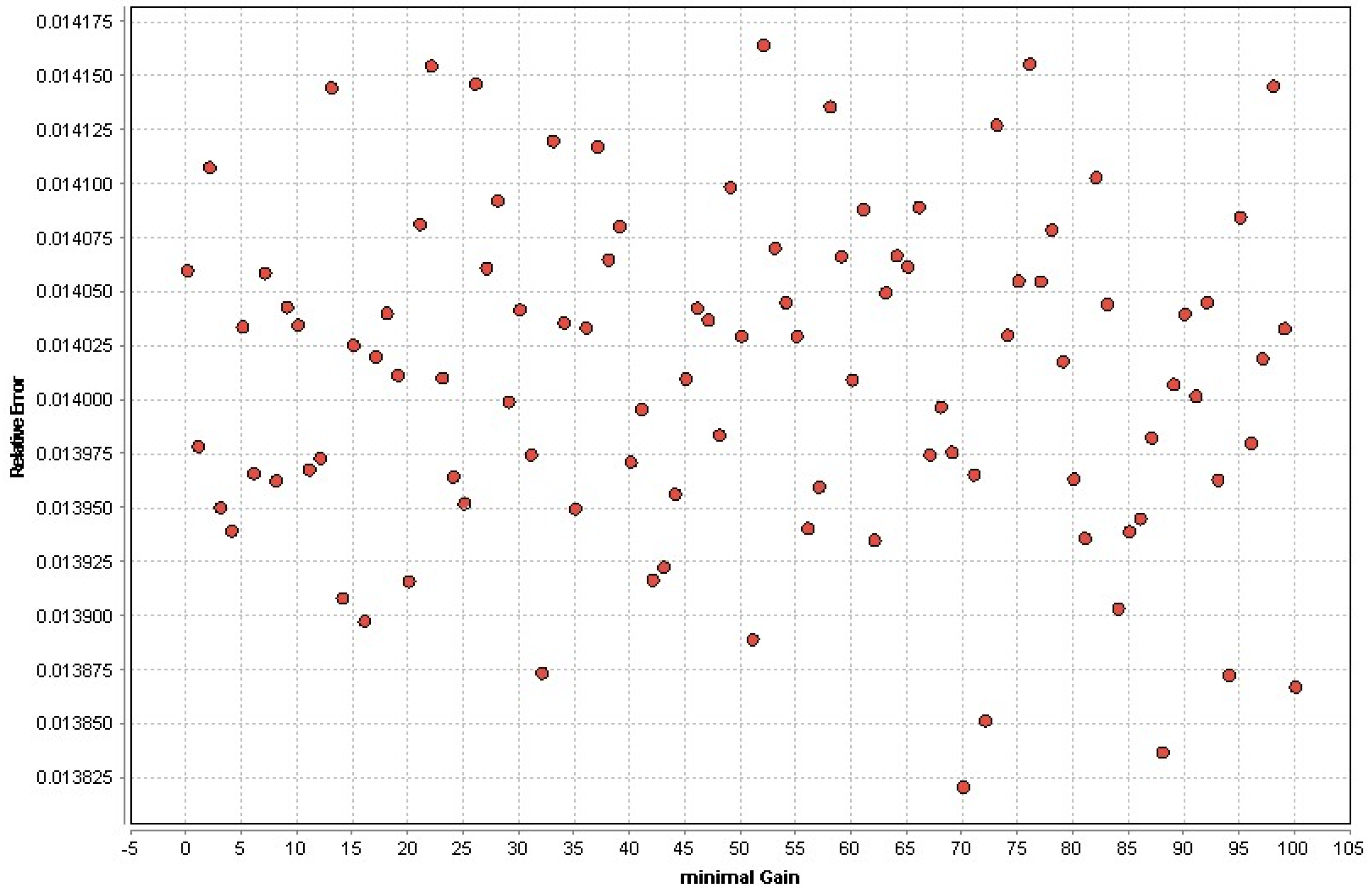
• Minimal gain: Before dividing a node, its gain is determined. If the node’s gain exceeds the minimal gain, it is divided. A greater minimal gain value means fewer splits and, as a result, a smaller tree. A value that is too high prevents splitting fully, resulting in a single-node tree.
• Minimal leaf size: The number of Examples in a leaf’s subset determines its size. Every leaf has at least the minimum leaf size number of Examples when the tree is constructed.
• Minimal size for split: The number of Examples in a node’s subset determines its size. Only nodes with a size larger than or equal to the split parameter’s minimum size are split.
• Number of prepruning alternatives: This option adjusts the amount of alternative nodes tested for splitting when split is stopped by prepruning at a specific node. As the tree creation process is paralleled by prepruning, this occurs. This could prohibit splitting at certain nodes if splitting at that node does not improve the tree’s discriminative capacity. Alternative nodes are tried for splitting in this situation.

3.5. Random Forest

3.5.1. Definition

Random forest is a supervised technique that consists of a bagging framework and an independent decision tree (DT). The core of random forest is the integration of DTs, which creates several DTs by randomizing column variables and row values in the dataset and then averaging the DTs’ results. To avoid slowing the tree’s growth, the pruning technique is not used when constructing the DT. Each tree is made up of column variables and row observations that are chosen at random. A single DT is difficult to predict accurately, but all DTs form a forest, allowing the aggregated findings to incorporate the outcomes of all DTs, resulting in a more accurate overall prediction [59].

3.5.2. Random Forest Parameters

The RF’s parameters are quite similar to those of DT, some of the other main parameters for this model [60] are:

• Number of trees: The number of random trees to generate is specified by this parameter. Bootstrapping is used to select a subset of Examples for each tree. The trees are trained in parallel across available processor threads if the parameter enable parallel execution is checked.
• Confidence: This option sets the level of confidence utilized in the pruning pessimistic error calculation.
• Random splits: If this parameter is enabled, numerical Attribute splits are picked at random rather than being optimized. A uniform sample between the least and maximal value for the current Attribute is conducted for random selection.

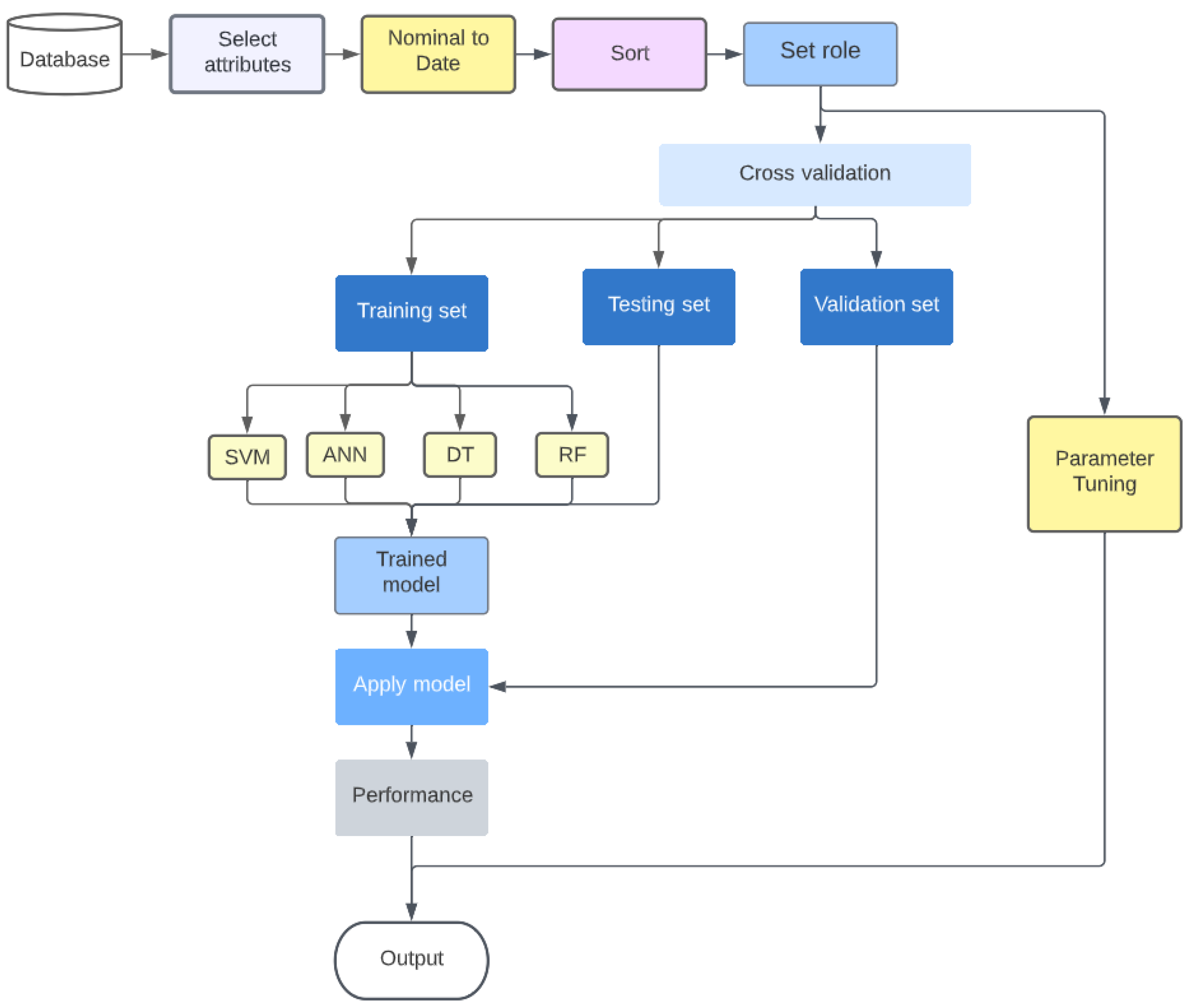
3.6. Rapid Miner

Rapid Miner is software that was created by Ralf Klinkenberg, Ingo Mierswa, and Simon Fischer in 2001 and was previously known as YALE (Yet Another Learning Environment). Statistical modeling, data preprocessing, business analysis, optimization, and prediction analysis are all performed by it. It has the following operators and repositories: Process control, Utility, Repository access, Import, Export, Data transformation, Modeling, and Evaluation [61].

In this section, we used RapidMiner Studio Educational 9.10.001.

In the Design View of RapidMiner Studio, your whiteboard workflow is implemented in software. There are many panels in the Design View.

• The Repository stores data, procedures, and results.
• Operators are the critical components of any workflow.
• Operators are linked through ports. The first’s output is used as the second’s input.
• An Operator’s behavior can be altered by altering its settings.
• Reading the Help can help you understand how an Operator behaves.

We applied the approach shown in Figure 7 to the cleaned data after importing it to Rapid Miner.

The stream of the process is depicted in Figure 8. The dataset comprises several attributes such as current, voltage, frequency, power, and power factor. The Select Attributes Operator selects a subset of a dataset’s Attributes while removing the rest. The date-time, apparent power, and active power are the attributes we have chosen in this situation. We used the Nominal to Date Operator to convert the date-time attribute’s type so that it could be used later because it was deemed a nominal parameter in the Rapid Miner. This operator converts the selected nominal attribute into the desired date-time type. Date and/or time values are converted from nominal values. This conversion is conducted with respect to the specified date format string. The Sort Operator is used to sort the input data set by date-time attribute in ascending order. Set role Operator changes the role of one or more Attributes, in our case we set the active power as the prediction target. Optimize Parameter (Grid) is used to tune the subprocess parameters for best performance outcome. Cross validation is used to estimate a learning model’s statistical performance. The dataset is split into a training and testing set within this operator, as seen in Figure 6. During the training phase, we deployed four different models: SVM, ANN, DT, and RF. In the testing phase, we apply the model on the testing Dataset using the Apply Model Operator. The trained model is then applied to the validation set to evaluate the model and measure its performance using the Performance Operator.

3.7. Performance Metrics

Different metrics are used to analyze the disparity between predicted and observed labels in a test dataset; these metrics allow us to test the performance of trained ML models on holdout data.

The suggested models’ prediction performance was assessed using R, MAE, RMSE, and RRSE metrics; Equations (2)–(5) are their corresponding formulations.

3.7.1. Correlation Coefficient

The correlation coefficient is a metric for how well two sets of data are related linearly. It is the product of two variables’ covariances and their standard deviations; consequently, it is effectively a normalized measurement of covariance, with the result always falling between −1 and 1. A perfect negative correlation is represented by a value of −1, whereas a perfect positive correlation is represented by a value of 1. A correlation of 0 indicates that the two variables’ movements have no linear relationship [62].

$$R=\frac{n{{\displaystyle \sum }}^{}y·y^{\prime }-({{\displaystyle \sum }}^{}y)({{\displaystyle \sum }}^{}{y}^{\prime })}{\sqrt{n({{\displaystyle \sum }}^{}y²)-({{\displaystyle \sum }}^{}y)²}\sqrt{n({{\displaystyle \sum }}^{}{y}^{\prime }²)-({{\displaystyle \sum }}^{}{y}^{\prime })²}}$$

(2)

where y’ is the predicted value, y represents the actual value, and n represents the number of data samples

3.7.2. Mean Absolute Error

The mean absolute error (MAE) is a metric for comparing errors between paired observations that describe the same occurrence. The MAE is determined by multiplying the following formula:

$$\mathrm{MAE}=\frac{1}{n}{\displaystyle \sum }_{i=1}^n\left|y-y^{\prime }\right|$$

(3)

The mean absolute error is calculated using the same scale as the data. Because this is a scale-dependent accuracy metric, it cannot be used to compare series with various scales. In time series analysis, the mean absolute error is a popular way to measure forecast error [63].

3.7.3. Root Mean Square Error

The root mean square error (RMSE) is a commonly used measure of the variations between values predicted by a model or estimator and the values observed. Because RMSE is scale-dependent, it is used to evaluate forecasting errors of different models for a single dataset rather than across datasets [64].

$$\mathrm{RMSE}=\sqrt{\frac{1}{n}{\displaystyle \sum }_{i=1}^n\left(y^{\prime }-y\right)²}$$

(4)

3.7.4. Root Relative Squared Error

The root relative squared error (RRSE) is a measure of how accurate a simple predictor would have been. This simple predictor is equal to the average of the actual values. As a result, the relative squared error normalizes the total squared error by dividing it by the simple predictor’s total squared error. The error is reduced to the same dimensions as the quantity being predicted by calculating the square root of the relative squared error [65].

The root relative squared error RRSE of an individual model I is calculated mathematically using the equation:

$$RRSE=\sqrt{\frac{{{\displaystyle \sum }}_{i=1}^n\left(y^{\prime }-y\right)²}{{{\displaystyle \sum }}_{i=1}^n\left(y-\overline{y}\right)²}}$$

(5)

where $\overline{y}$ is given by the formula:

$$\overline{y}=\frac{1}{n}{\displaystyle \sum }_{i=1}^{n}y$$

4. Results and Discussion

Table 2. Default settings of model parameters in RapidMiner Studio.

Model	Parameters	Default Value
SVM	Kernel type	Dot
	Kernel cache	200
	C	0.0
	Convergence epsilon	0.001
	Max iterations	100,000
ANN	Hidden layers size	2
	Training cycle	200
	Learning rate	0.01
	Momentum	0.9
DT	Criterion	Least square
	Maximal depth	10
	Minimal gain	0.01
	Minimal leaf size	2
	Minimal size for split	4
	Number of prepruning alternatives	3
RF	Number of trees	100
	Criterion	Least square
	Maximal depth	10

shows the models’ parameters of the four machine learning algorithms used in this comparative study before parameter tuning; these parameters present the default settings in Rapid miner.

4.1. Parameter Tuning Results

The Optimize Parameter operator is used to tune the selected parameters within its subprocess. We chose to tune one single parameter for each model that has an impact on the performance to see the effect of this procedure on the final results.

At this stage, we appoint the minimal gain parameter for the Decision Tree (Figure 9) and Random Forest (Figure 10), the training cycles parameter for the Artificial Neural Network (Figure 11), and the convergence epsilon for the Support Vector Machine (Figure 12).

Table 3. Parameter tuning results.

Model	Parameter	Tuned Value
DT	Minimal gain	0.0595
RF	Minimal gain	70
ANN	Training cycles	164
SVM	Convergence epsilon	88

summarize the obtained results after the parameters tuning for all four models. We notice that the minimal gain for Decision Tree tends to engender the lowest relative error with a value of 0.0595; while for Random Forest it produces the best performance with a value of 70. The Artificial Neural Network model presents best results when the training cycles equal 164. The convergence epsilon is estimated to 88, giving the lowest RMSE value for the Support Vector Machine model.

4.2. Performance Results

The four models’ performance measures R, MAE, RMSE and RRSE are summarized in the

Table 4. Performance results of the four models.

Model	Measure	Before Optimization		After Optimization
		Testing Set	Validation Set	Testing Set	Validation Set
SVM	R	0.984	0.994	0.984	0.994
	MAE	0.0368	0.0291	0.0365	0.0282
	RMSE	518.695	421.49	516.44	415.86
	RRSE	0.183	0.112	0.182	0.111
ANN	R	0.992	0.995	0.992	0.995
	MAE	0.0265	0.0276	0.0267	0.0290
	RMSE	365.192	381.256	363.48	384.745
	RRSE	0.129	0.101	0.128	0.102
DT	R	0.997	0.966	0.999	1
	MAE	0.0093	0.0474	0.0050	0.0041
	RMSE	200.763	985.602	116.139	94.175
	RRSE	0.071	0.262	0.031	0.025
RF	R	0.998	0.971	1	1
	MAE	0.0079	0.0516	0.0038	0.0027
	RMSE	186.057	939.576	92.196	52.16
	RRSE	0.065	0.25	0.025	0.014

Note: Bold value denotes the best performance.

. The chart depicts the obtained results with the testing set and validation set before and after parameter tuning. The best performance for energy forecasting is obtained by the Random Forest algorithm followed by Decision Tree, Artificial Neural Network and then the Support Vector Machine algorithm.

4.3. Statistical Results

The statistical results of the power prediction (Prediction (P(W)) after parameter tuning compared to the original Data of power (P(W)) achieved with SVM in Figure 13, ANN in Figure 14, DT in Figure 15, and RF in Figure 16 are shown in the charts below from Rapid Miner.

The charts present a description of different attributes of our dataset namely the power (P(W), the predicted power, the apparent power (S(VA)), and the time. These results show the type of the attribute, the missing values of this attribute in the dataset, the min, max, and average values of the attribute.

We can see that, when compared to the other three models, the RF model delivers values of predicted power that are quite close to the ones obtained from the actual data.

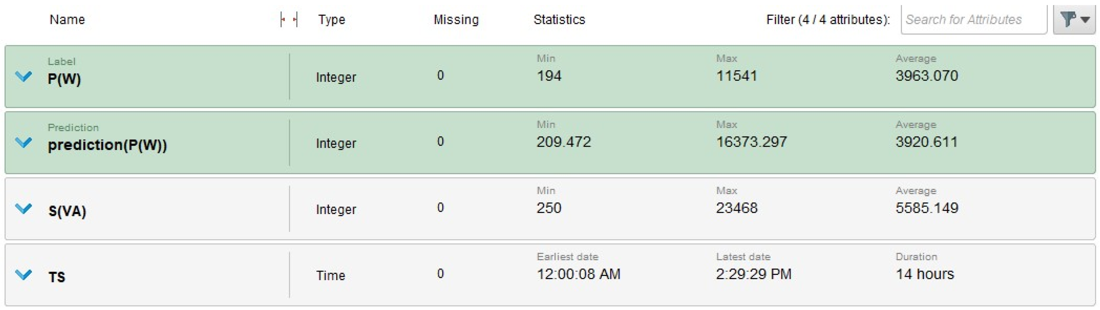
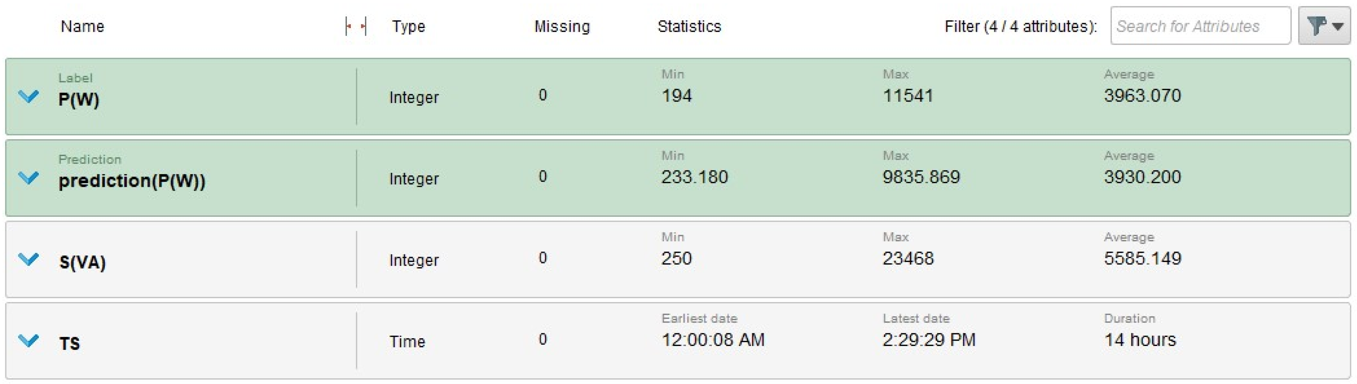
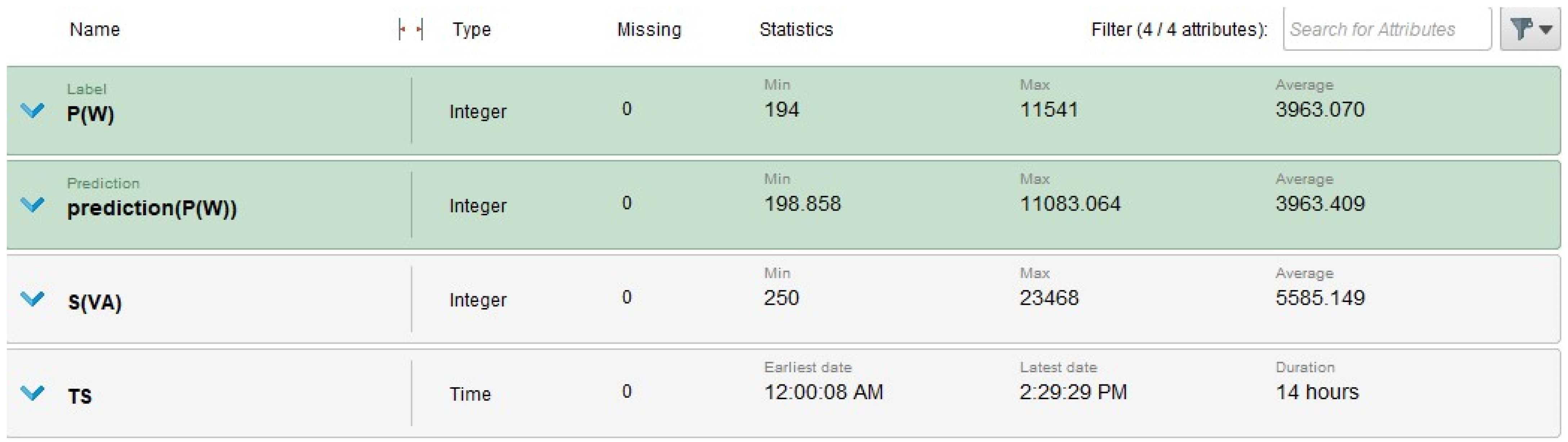
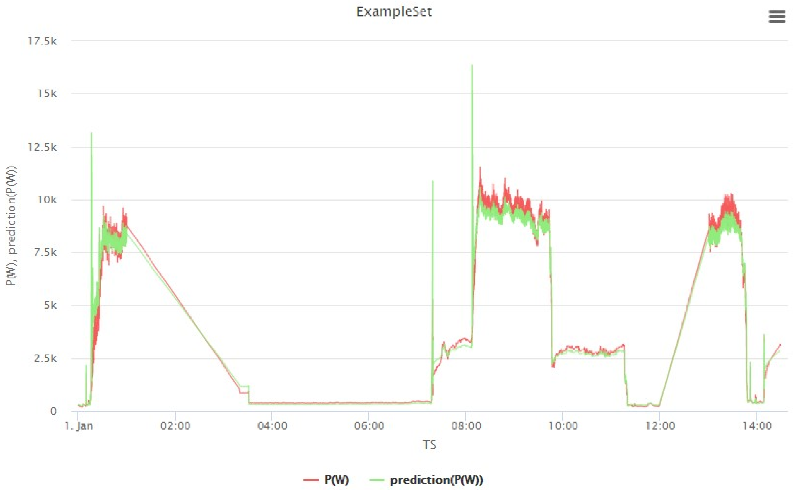
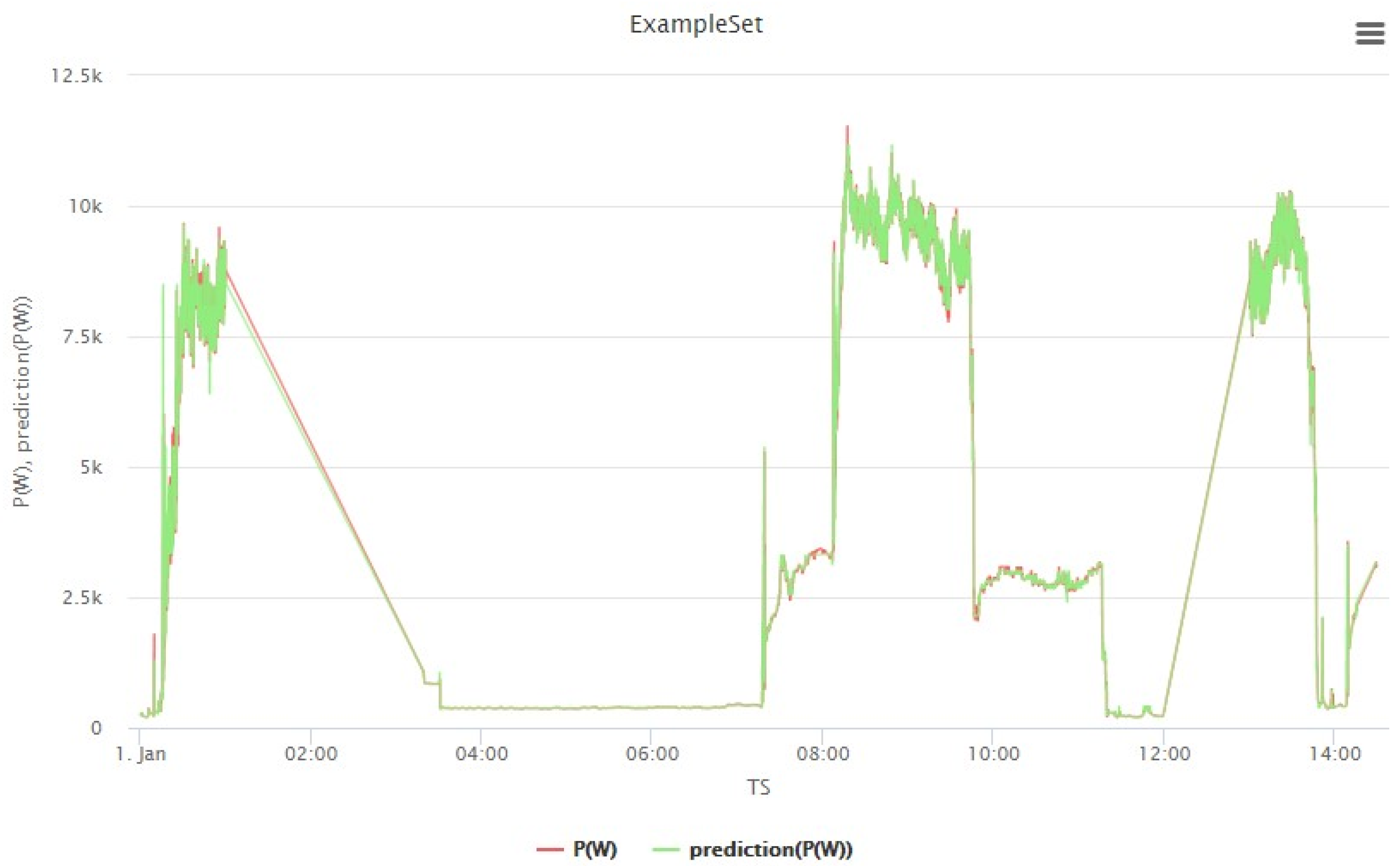
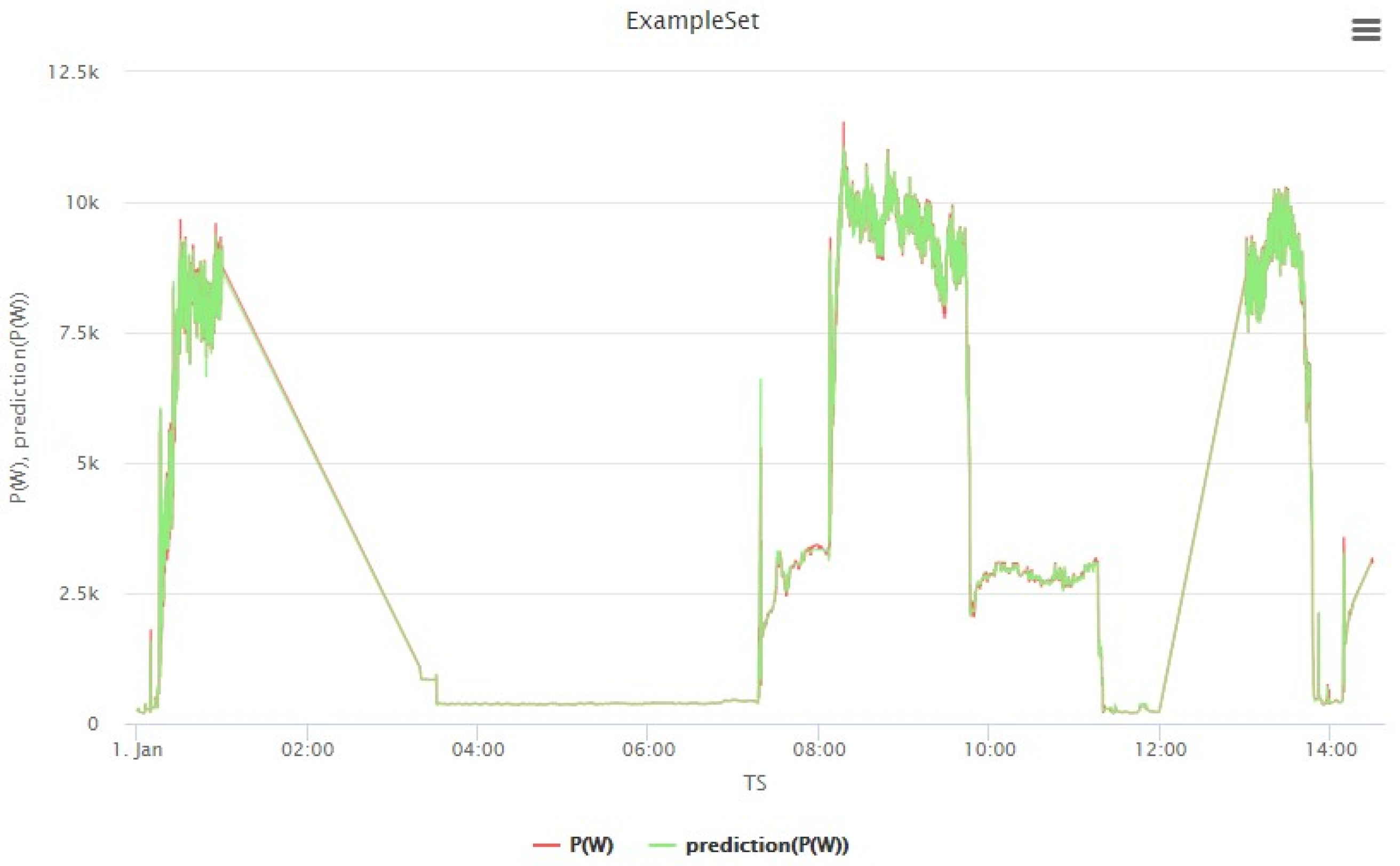
4.4. Visualization Results

RapidMiner was used to create a visualization of the original and forecasted data that displays the behavior of our prediction models after parameter tuning, as seen in Figure 17 for the SVM model, Figure 18 for the ANN model, Figure 19 for the DT model, and Figure 20 for the RF model. By looking at the four representations, we can observe that the graph of the RF model has the best prediction behavior, followed by DT, then ANN, and finally SVM.

Based on data acquired over 24 h from the experimental open-pit mine, this study is established in order to identify the best of SVM, ANN, DT, and RF models for power forecasting in similar cases. The statistical results, visualizations, and performance metrics all show that the RF model produced the best results among the three models in RapidMiner Studio, with the best values for all evaluation measures.

According to the ISO 50001 norm, energy demand forecasting is a key instrument with a low-cost investment for improving energy efficiency in businesses. As a result of this research, the open-pit mine’s energy managers will be provided annually to hourly estimates of energy consumption, which will enable them to review the energy budget and negotiate effectively with the finance team and the utility company. The significance of the entire process stems from the fact that the industry is penalized if it exceeds the stipulated energy or does not consume the allotted energy within a particular tolerance rate. The tested method with the best performance has a very low error rate, ensuring good energy forecasting precision.

Furthermore, technicians and supervisors will not only be able to view real-time energy consumption, but will also be able to analyze future warnings based on the current condition of load consumption and make timely decisions.

Finally, this forecasting method may be used to investigate the behavior of experimental open-pit mine loads and simulate extreme scenarios in order to determine the best production Key performance indicators (KPIs), which is an important component of the digital twin.

5. Conclusions

Energy management is critical for the mining industry to reduce its energy use. The value of energy conservation stems from the global desire to reduce energy use and environmental implications, as well as related legislation. Many trials have recently been conducted by utilizing machine learning approaches using data on energy use in operational and residential buildings, but there has been insufficient research into forecasting energy consumption in the mining industry.

This study presents a comprehensive approach to applying ML models for mine energy consumption forecasts using RapidMiner tool. The goal of this study is to determine the best effective model for a variety of users who must quickly construct predictive models. This research examines some of the forecasting approaches available for this problem and makes recommendations for their appropriate application.

Four machine learning techniques namely, Support Vector Machine, Artificial Neural Network, Decision Tree, and Random Forest were used in this study to forecast the energy consumption of an experimental open-pit mine based on real-time data acquired over 24 h. The performance of the different models was assessed and evaluated using four metrics, namely R, MAE, RMSE, and RRSE. The RF model outperformed the SVM, ANN and DT models in a thorough comparison.

For future work, the prediction process will be merged into an existing monitoring system to make energy forecasting easier for users. The acquisition of more data will enable us to make long-term forecasts, and this additional data may then be used to detect anomalous behavior and identify system failures using a classification model which can be added and co-simulate different scenarios simultaneously in a smart grid framework which was presented in recent work, these models can be configured within a test bench in order to predict and optimize the power flow in different case studies [66]. The energy expenses and production earnings can then be correlated.

References

1. OECD. Key World Energy Statistics 2015; Organisation for Economic Co-Operation and Development: Paris, France, 2015. [Google Scholar]
2. Statistical Review of World Energy, Energy Economics, Home Page. Available online: https://www.bp.com/en/global/corporate/energy-economics/statistical-review-of-world-energy.html (accessed on 28 February 2022).
3. Darling, P. Mining: Ancient, modern and beyond. In SME Mining Engineering Handbook; Society for Mining, Metallurgy, and Exploration, Inc.: Englewood, CO, USA, 2011; pp. 3–9. [Google Scholar]
4. Open Pit Mining|IntechOpen. Available online: https://www.intechopen.com/chapters/71931 (accessed on 29 April 2022).
5. Grewal, G.S.; Rajpurohit, B.S. Efficient Energy Management Measures in Steel Industry for Economic Utilization. Energy Rep. 2016, 2, 267–273. [Google Scholar] [CrossRef] [Green Version]
6. Norgate, T.; Haque, N. Energy and Greenhouse Gas Impacts of Mining and Mineral Processing Operations. J. Clean. Prod. 2010, 18, 266–274. [Google Scholar] [CrossRef]
7. Rábago, K.R.; Lovins, A.B.; Feiler, T.E. Energy and Sustainable Development in the Mining and Minerals Industrie; Report for The Mining, Minerals and Sustainable Development Project; Rocky Mountain Institute: Snowmass Village, CO, USA, 2001. [Google Scholar]
8. Marimon, F.; Casadesús, M. Reasons to Adopt ISO 50001 Energy Management System. Sustainability 2017, 9, 1740. [Google Scholar] [CrossRef] [Green Version]
9. Hasan, A.S.M.M.; Trianni, A. A Review of Energy Management Assessment Models for Industrial Energy Efficiency. Energies 2020, 13, 5713. [Google Scholar] [CrossRef]
10. Yan, K.; Zhou, X.; Chen, J. Collaborative Deep Learning Framework on IoT Data with Bidirectional NLSTM Neural Networks for Energy Consumption Forecasting. J. Parallel Distrib. Comput. 2022, 163, 248–255. [Google Scholar] [CrossRef]
11. Biswas, M.A.R.; Robinson, M.D.; Fumo, N. Prediction of Residential Building Energy Consumption: A Neural Network Approach. Energy 2016, 117, 84–92. [Google Scholar] [CrossRef]
12. Jin, N.; Yang, F.; Mo, Y.; Zeng, Y.; Zhou, X.; Yan, K.; Ma, X. Highly Accurate Energy Consumption Forecasting Model Based on Parallel LSTM Neural Networks. Adv. Eng. Inform. 2022, 51, 101442. [Google Scholar] [CrossRef]
13. González-Briones, A.; Hernández, G.; Corchado, J.M.; Omatu, S.; Mohamad, M.S. Machine Learning Models for Electricity Consumption Forecasting: A Review. In Proceedings of the 2019 2nd International Conference on Computer Applications Information Security (ICCAIS), Riyadh, Saudi Arabia, 1–3 May 2019; pp. 1–6. [Google Scholar]
14. Marino, D.L.; Amarasinghe, K.; Manic, M. Building Energy Load Forecasting Using Deep Neural Networks. In Proceedings of the IECON 2016—42nd Annual Conference of the IEEE Industrial Electronics Society, Florence, Italy, 23–26 October 2016; pp. 7046–7051. [Google Scholar]
15. Kong, W.; Dong, Z.Y.; Jia, Y.; Hill, D.J.; Xu, Y.; Zhang, Y. Short-Term Residential Load Forecasting Based on LSTM Recurrent Neural Network. IEEE Trans. Smart Grid 2019, 10, 841–851. [Google Scholar] [CrossRef]
16. Kim, T.-Y.; Cho, S.-B. Predicting Residential Energy Consumption Using CNN-LSTM Neural Networks. Energy 2019, 182, 72–81. [Google Scholar] [CrossRef]
17. Wu, B.; Wang, L.; Wang, S.; Zeng, Y.-R. Forecasting the U.S. Oil Markets Based on Social Media Information during the COVID-19 Pandemic. Energy 2021, 226, 120403. [Google Scholar] [CrossRef]
18. Somu, N.; Raman, M.R.G.; Ramamritham, K. A Deep Learning Framework for Building Energy Consumption Forecast. Renew. Sustain. Energy Rev. 2021, 137, 110591. [Google Scholar] [CrossRef]
19. Liu, L.; Wu, L. Forecasting the Renewable Energy Consumption of the European Countries by an Adjacent Non-Homogeneous Grey Model. Appl. Math. Model. 2021, 89, 1932–1948. [Google Scholar] [CrossRef]
20. Liu, T.; Tan, Z.; Xu, C.; Chen, H.; Li, Z. Study on Deep Reinforcement Learning Techniques for Building Energy Consumption Forecasting. Energy Build. 2020, 208, 109675. [Google Scholar] [CrossRef]
21. Singh, S.; Yassine, A. Big Data Mining of Energy Time Series for Behavioral Analytics and Energy Consumption Forecasting. Energies 2018, 11, 452. [Google Scholar] [CrossRef] [Green Version]
22. Boogen, N.; Datta, S.; Filippini, M. Dynamic Models of Residential Electricity Demand: Evidence from Switzerland. Energy Strategy Rev. 2017, 18, 85–92. [Google Scholar] [CrossRef] [Green Version]
23. Abulibdeh, A. Modeling Electricity Consumption Patterns during the COVID-19 Pandemic across Six Socioeconomic Sectors in the State of Qatar. Energy Strategy Rev. 2021, 38, 100733. [Google Scholar] [CrossRef]
24. Laayati, O.; Bouzi, M.; Chebak, A. Smart Energy Management System: Design of a Monitoring and Peak Load Forecasting System for an Experimental Open-Pit Mine. Appl. Syst. Innov. 2022, 5, 18. [Google Scholar] [CrossRef]
25. Laayati, O.; Bouzi, M.; Chebak, A. Smart Energy Management: Energy Consumption Metering, Monitoring and Prediction for Mining Industry. In Proceedings of the 2020 IEEE 2nd International Conference on Electronics, Control, Optimization and Computer Science (ICECOCS), Kenitra, Morocco, 2–3 December 2020; pp. 1–5. [Google Scholar]
26. Solomon, D.; Winter, R.; Boulanger, A.; Anderson, R.; Wu, L. Forecasting Energy Demand in Large Commercial Buildings Using Support Vector Machine Regression; CUCS-040-11; Department of Computer Science, Columbia University: New York, NY, USA, 2011. [Google Scholar]
27. Edwards, R.E.; New, J.; Parker, L.E. Predicting Future Hourly Residential Electrical Consumption: A Machine Learning Case Study. Energy Build. 2012, 49, 591–603. [Google Scholar] [CrossRef]
28. Dagnely, P.; Ruette, T.; Tourwé, T.; Tsiporkova, E.; Verhelst, C. Predicting Hourly Energy Consumption. Can Regression Modeling Improve on an Autoregressive Baseline? In Proceedings of the Data Analytics for Renewable Energy Integration; Woon, W.L., Aung, Z., Madnick, S., Eds.; Springer International Publishing: Cham, Switzerland, 2015; pp. 105–122. [Google Scholar]
29. Massana, J.; Pous, C.; Burgas, L.; Melendez, J.; Colomer, J. Short-Term Load Forecasting in a Non-Residential Building Contrasting Models and Attributes. Energy Build. 2015, 92, 322–330. [Google Scholar] [CrossRef] [Green Version]
30. Borges, C.; Penya, Y.; Agote, D.; Fernandez, I. Short-Term Load Forecasting in Non-Residential Buildings. In Proceedings of the IEEE Africon’11 Conference, Victoria Falls, Zambia, 13–15 September 2011. [Google Scholar]
31. Zhao, H.X.; Magoulès, F. Parallel Support Vector Machines Applied to the Prediction of Multiple Buildings Energy Consumption. 2010. Available online: https://0-journals-sagepub-com.brum.beds.ac.uk/doi/10.1260/1748-3018.4.2.231 (accessed on 28 February 2022).
32. Paudel, S.; Nguyen, P.H.; Kling, W.L.; Elmitri, M.; Lacarrière, B.; Corre, O.L. Support Vector Machine in Prediction of Building Energy Demand Using Pseudo Dynamic Approach. arXiv 2015, arXiv:1507.05019. [Google Scholar]
33. Jain, R.K.; Smith, K.; Culligan, P.J.; Taylor, J.E. Forecasting Energy Consumption of Multi-Family Residential Buildings Using Support Vector Regression: Investigating the Impact of Temporal and Spatial Monitoring Granularity on Performance Accuracy. Appl. Energy 2014, 123, 168–178. [Google Scholar]
34. Mena, R.; Rodríguez, F.; Castilla, M.; Arahal, M.R. A Prediction Model Based on Neural Networks for the Energy Consumption of a Bioclimatic Building. Energy Build. 2014, 82, 142–155. [Google Scholar] [CrossRef]
35. Penya, Y.K.; Borges, C.E.; Agote, D.; Fernández, I. Short-term load forecasting in air-conditioned non-residential Buildings. In Proceedings of the 2011 IEEE International Symposium on Industrial Electronics, Gdansk, Poland, 27–30 June 2011; pp. 1359–1364. [Google Scholar] [CrossRef] [Green Version]
36. González, P.A.; Zamarreño, J. Prediction of Hourly Energy Consumption in Buildings Based on a Feedback Artificial Neural Network. Energy Build. 2005, 37, 595–601. Available online: https://0-www-sciencedirect-com.brum.beds.ac.uk/science/article/pii/S0378778804003032 (accessed on 9 March 2022). [CrossRef]
37. Fernández, I.; Borges, C.E.; Penya, Y.K. Efficient Building Load Forecasting. In Proceedings of the ETFA2011, Toulouse, France, 5–9 September 2011; pp. 1–8. [Google Scholar]
38. Escrivá-Escrivá, G.; Álvarez-Bel, C.; Roldán-Blay, C.; Alcázar-Ortega, M. New Artificial Neural Network Prediction Method for Electrical Consumption Forecasting Based on Building End-Uses. Energy Build. 2011, 43, 3112–3119. [Google Scholar] [CrossRef]
39. Kamaev, V.A.; Shcherbakov, M.V.; Panchenko, D.P.; Shcherbakova, N.L.; Brebels, A. Using Connectionist Systems for Electric Energy Consumption Forecasting in Shopping Centers. Autom. Remote Control 2012, 73, 1075–1084. [Google Scholar] [CrossRef]
40. Bagnasco, A.; Fresi, F.; Saviozzi, M.; Silvestro, F.; Vinci, A. Electrical Consumption Forecasting in Hospital Facilities: An Application Case. Energy Build. 2015, 103, 261–270. [Google Scholar] [CrossRef]
41. Borges, C.E.; Penya, Y.K.; Fernández, I.; Prieto, J.; Bretos, O. Assessing Tolerance-Based Robust Short-Term Load Forecasting in Buildings. Energies 2013, 6, 2110–2129. [Google Scholar] [CrossRef] [Green Version]
42. Lai, F.; Magoulés, F.; Lherminier, F. Vapnik’s Learning Theory Applied to Energy Consumption Forecasts in Residential Buildings. Int. J. Comput. Math. 2008, 85, 1563–1588. [Google Scholar]
43. Farzana, S.; Liu, M.; Baldwin, A.; Hossain, M.U. Multi-Model Prediction and Simulation of Residential Building Energy in Urban Areas of Chongqing, South West China. Energy Build. 2014, 81, 161–169. [Google Scholar] [CrossRef]
44. Yuan, J.; Farnham, C.; Azuma, C.; Emura, K. Predictive Artificial Neural Network Models to Forecast the Seasonal Hourly Electricity Consumption for a University Campus. Sustain. Cities Soc. 2018, 42, 82–92. [Google Scholar] [CrossRef]
45. Peng, Y.; Liu, H.; Li, X.; Huang, J.; Wang, W. Machine Learning Method for Energy Consumption Prediction of Ships in Port Considering Green Ports. J. Clean. Prod. 2020, 264, 121564. [Google Scholar] [CrossRef]
46. Shao, M.; Wang, X.; Bu, Z.; Chen, X.; Wang, Y. Prediction of Energy Consumption in Hotel Buildings via Support Vector Machines. Sustain. Cities Soc. 2020, 57, 102128. [Google Scholar] [CrossRef]
47. Wu, X.; Kumar, V.; Ross Quinlan, J.; Ghosh, J.; Yang, Q.; Motoda, H.; McLachlan, G.J.; Ng, A.; Liu, B.; Yu, P.S.; et al. Top 10 Algorithms in Data Mining. Knowl. Inf. Syst. 2008, 14, 1–37. [Google Scholar] [CrossRef] [Green Version]
48. Zhao, H.; Magoulès, F. A Review on the Prediction of Building Energy Consumption. Renew. Sustain. Energy Rev. 2012, 16, 3586–3592. [Google Scholar] [CrossRef]
49. Wei, Y.; Zhang, X.; Shi, Y.; Xia, L.; Pan, S.; Wu, J.; Han, M.; Zhao, X. A Review of Data-Driven Approaches for Prediction and Classification of Building Energy Consumption. Renew. Sustain. Energy Rev. 2018, 82, 1027–1047. [Google Scholar] [CrossRef]
50. RapidMiner Documentation. Support Vector Machine. Available online: https://docs.rapidminer.com/latest/studio/operators/modeling/predictive/support_vector_machines/support_vector_machine.html (accessed on 1 March 2022).
51. Amasyali, K.; El-Gohary, N.M. A Review of Data-Driven Building Energy Consumption Prediction Studies. Renew. Sustain. Energy Rev. 2018, 81, 1192–1205. [Google Scholar] [CrossRef]
52. Bourhnane, S.; Abid, M.R.; Lghoul, R.; Zine-Dine, K.; Elkamoun, N.; Benhaddou, D. Machine Learning for Energy Consumption Prediction and Scheduling in Smart Buildings. SN Appl. Sci. 2020, 2, 297. [Google Scholar] [CrossRef] [Green Version]
53. Bourdeau, M.; Zhai, X.Q.; Nefzaoui, E.; Guo, X.; Chatellier, P. Modeling and Forecasting Building Energy Consumption: A Review of Data-Driven Techniques. Sustain. Cities Soc. 2019, 48, 101533. [Google Scholar] [CrossRef]
54. Ahmad, M.W.; Mourshed, M.; Rezgui, Y. Trees vs. Neurons: Comparison between Random Forest and ANN for High-Resolution Prediction of Building Energy Consumption. Energy Build. 2017, 147, 77–89. [Google Scholar] [CrossRef]
55. RapidMiner Documentation. Neural Net. Available online: https://docs.rapidminer.com/latest/studio/operators/modeling/predictive/neural_nets/neural_net.html (accessed on 1 March 2022).
56. Domingos, P. A Few Useful Things to Know about Machine Learning. Commun. ACM 2012, 55, 78–87. [Google Scholar] [CrossRef] [Green Version]
57. Yu, Z.; Haghighat, F.; Fung, B.C.M.; Yoshino, H. A Decision Tree Method for Building Energy Demand Modeling. Energy Build. 2010, 42, 1637–1646. [Google Scholar] [CrossRef] [Green Version]
58. RapidMiner Documentation. Decision Tree. Available online: https://docs.rapidminer.com/latest/studio/operators/modeling/predictive/trees/parallel_decision_tree.html (accessed on 1 March 2022).
59. Dai, Y.; Khandelwal, M.; Qiu, Y.; Zhou, J.; Monjezi, M.; Yang, P. A Hybrid Metaheuristic Approach Using Random Forest and Particle Swarm Optimization to Study and Evaluate Backbreak in Open-Pit Blasting. Neural Comput. Appl. 2022, 34, 6273–6288. [Google Scholar] [CrossRef]
60. RapidMiner Documentation. Random Forest. Available online: https://docs.rapidminer.com/latest/studio/operators/modeling/predictive/trees/parallel_random_forest.html (accessed on 31 March 2022).
61. Yadav, A.K.; Malik, H.; Chandel, S.S. Application of Rapid Miner in ANN Based Prediction of Solar Radiation for Assessment of Solar Energy Resource Potential of 76 Sites in Northwestern India. Renew. Sustain. Energy Rev. 2015, 52, 1093–1106. [Google Scholar] [CrossRef]
62. Correlation Coefficient: Simple Definition, Formula, Easy Calculation Steps. Available online: https://www.statisticshowto.com/probability-and-statistics/correlation-coefficient-formula/ (accessed on 23 February 2022).
63. Willmott, C.J.; Matsuura, K. Advantages of the mean absolute error (MAE) over the root mean square error (RMSE) in assessing average model performance. Clim. Res. 2005, 30, 79–82. [Google Scholar] [CrossRef]
64. Hyndman, R.J.; Koehler, A.B. Another Look at Measures of Forecast Accuracy. Int. J. Forecast. 2006, 22, 679–688. [Google Scholar] [CrossRef] [Green Version]
65. Root Relative Squared Error. Available online: https://www.gepsoft.com/GeneXproTools/AnalysesAndComputations/MeasuresOfFit/RootRelativeSquaredError.htm (accessed on 21 February 2022).
66. Laayati, O.; El Hadraoui, H.; Guennoui, N.; Bouzi, M.; Chebak, A. Smart Energy Management System: Design of a Smart Grid Test Bench for Educational Purposes. Energies 2022, 15, 2702. [Google Scholar] [CrossRef]
Figure 1. Flowchart of the followed methodology.
Energies 15 04569 g001
Figure 2. Energy consumption behavior during 24 h.
Energies 15 04569 g002
Figure 3. SVM algorithm flowchart.
Energies 15 04569 g003
Figure 4. Feed forward neural network architecture.
Energies 15 04569 g004
Figure 5. Decision Tree approach.
Energies 15 04569 g005
Figure 6. Decision Tree flowchart.
Energies 15 04569 g006
Figure 7. Stream of the process in RapidMiner Studio.
Energies 15 04569 g007
Figure 8. Flowchart of the process stream.
Energies 15 04569 g008
Figure 9. Minimal gain tuning results for Decision Tree model.
Energies 15 04569 g009
Figure 10. Minimal gain tuning results for Random Forest model.
Energies 15 04569 g010
Figure 11. Training cycles tuning results for ANN model.
Energies 15 04569 g011
Figure 12. Convergence epsilon tuning results for SVM model.
Energies 15 04569 g012
Figure 13. Statistical results of SVM model.
Energies 15 04569 g013
Figure 14. Statistical results of ANN model.
Energies 15 04569 g014
Figure 15. Statistical results of DT model.
Energies 15 04569 g015
Figure 16. Statistical results of RF model.
Energies 15 04569 g016
Figure 17. Visualization graph of SVM model.
Energies 15 04569 g017
Figure 18. Visualization graph of ANN model.
Energies 15 04569 g018
Figure 19. Visualization graph of DT model.
Energies 15 04569 g019
Figure 20. Visualization graph of RF model.
Energies 15 04569 g020