
Life Prediction under Charging Process of Lithium-Ion Batteries Based on AutoML
by
 ,
,
Chenqiang Luo
1,*, 
Zhendong Zhang
1,*,
Dongdong Qiao
2,
Xin Lai
1,
Yongying Li
1 and
Shunli Wang
3,4 1
College of Mechanical Engineering, University of Shanghai for Science and Technology, Shanghai 200093, China
2
School of Automotive Studies, Tongji University, Shanghai 201804, China
3
College of Electrical Engineering, Sichuan University, Chengdu 610065, China
4
School of Information Engineering, Southwest University of Science and Technology, Mianyang 621010, China
*
Authors to whom correspondence should be addressed.
Energies 2022, 15(13), 4594; https://0-doi-org.brum.beds.ac.uk/10.3390/en15134594
Submission received: 26 May 2022
/
Revised: 16 June 2022
/
Accepted: 21 June 2022
/
Published: 23 June 2022
(This article belongs to the Special Issue Application of Artificial Intelligence in Power System Monitoring and Fault Diagnosis)
Abstract
:Accurate online capacity estimation and life prediction of lithium-ion batteries (LIBs) are crucial to large-scale commercial use for electric vehicles. The data-driven method lately has drawn great attention in this field due to efficient machine learning, but it remains an ongoing challenge in the feature extraction related to battery lifespan. Some studies focus on the features only in the battery constant current (CC) charging phase, regardless of the joint impact including the constant voltage (CV) charging phase on the battery aging, which can lead to estimation deviation. In this study, we analyze the features of the CC and CV phases using the optimized incremental capacity (IC) curve, showing the strong relevance between the IC curve in the CC phase as well as charging capacity in the CV phase and battery lifespan. Then, the life prediction model based on automated machine learning (AutoML) is established, which can automatically generate a suitable pipeline with less human intervention, overcoming the problem of redundant model information and high computational cost. The proposed method is verified on NASA’s LIBs cycle life datasets, with the MAE increased by 52.8% and RMSE increased by 48.3% compared to other methods using the same datasets and training method, accomplishing an obvious enhancement in online life prediction with small-scale datasets.
1. Introduction
With the increasing reduction of fossil energy reserves and severe air pollution, considerable attention has been paid to electric vehicles (EVs) in recent years, which can be energy-saving and environmental-friendly solutions, whereas the traditional automobile industry is a big energy consumer, causing serious exhaust emission [1,2].
Lithium-ion batteries (LIBs) are the ideal energy storage device for EVs, and their safe and feasible application as a power source can contribute to their value in their entire lifespan, which can promote secondary utilization and material recycling, conducting the carbon footprint in the battery production and recycling stages [3]. Hence, the safety and reliability of LIBs in EVs have been spotlighted. However, unlike in the laboratory cycle, the battery performance and the available capacity degrades erratically due to random operation during driving, which could cause underuse or overuse of battery cells, leading to resource waste as well as some potential disasters without accurate remaining useful life (RUL) prediction. Consequently, life prediction and capacity estimation of LIBs are facing challenges, and it is worthwhile devoting much effort to elucidate the battery degradation evolution trend in lifespan, thus, avoiding premature replacement and excessive use.
The typical method of LIBs RUL prediction is usually divided into two categories: model-driven and data-driven methods. The model-driven method exploits the intrinsic aging mechanism and induces complex equations to reflect the reactions process. These models are often established in the theoretical derivation process using mechanism knowledge. Additionally, model parameters are identified through empirical assumptions and mathematical algorithms, such as extended Kalman filter (EKF) [4], expectation maximization (EM) [5], unscented particle filter (UPF) [6], and autoregressive moving average (ARMA) [7]. Nonetheless, it is difficult to predict precisely because of the complex nonlinear process and discrepancy between data distribution and model hypothesis.
The data-driven method has recently received significant attention in LIB’s RUL prediction because of easy access to data and the development of machine learning. The raw measured data during operation can serve as the learning model and bridge the implicit gap between the input and output data. More importantly, the successful application of some advanced learning algorithms in machine translation, speech recognition, and computer vision provides a remarkable applying reference for state estimation and RUL prediction in LIBs.
Data-driven methods for RUL prediction are cataloged as machine learning (ML), artificial neural network (ANN), and deep learning (DL). ML: Richardson et al. [8] proposed a regression of the Gaussian process (GP) algorithm for LIBs RUL prediction, with a good performance in long-term forecasting. Yun et al. [9] explored a hybrid prognosis approach for RUL estimation, combining the variational mode decomposition (VMD), autoregressive integrated moving average (ARIMA), and gray model (GM) models for RUL prediction. ANN: Zhang et al. [10] suggested a novel method based on ANN with four layers for state of health (SOH) estimation and RUL prediction using the incremental capacity curve during the constant current discharge phase. Sun et al. [11] proposed a cloud-edge collaborative strategy with state of health (SOH) for capacity estimation and back propagation neural network (BPNN) optimized by a genetic algorithm for capacity prediction. DL: Dong et al. [12] applied the long short-term memory (LSTM) for the RUL prediction, which can solve the gradient exploding problem during iterating. Zraibi et al. [13] pointed out a CNN-LSTM-DNN algorithm for RUL prediction, in which the three hybrid methods respectively play a critical role. Wang et al. [14] proposed a hybrid method combined with a BiLSTM-AM model and a support vector regression (SVR) model for online life prediction, and the collected initial data are updated by SVR, and BiLSTM-AM is used to predict cycle life. Tang et al. [15] decomposed the original data into high- and low-frequency parts precisely through an ensemble empirical mode decomposition, and the parts separately are predicted by DNN and a self-designed LSTM network, named IRes2Net-BiGRU-FC, which showed a high robustness of RUL prediction in both the CC and CV stages.
Currently, most of the research in RUL prediction currently focuses on the application of deep learning and their variant with an intricate network, which can overcome the vanishing and exploding gradient, over-fitting in training, and distortion in long-term dependence through architecture optimization and hyperparameters tuning, which has made outstanding accomplishments. However, some problems also occur, for example, it is difficult to achieve a good training speed and effect for small-scale data in short order due to unmatched model structure and human experts must be deeply involved in every segment of the designing model because of its knowledge- and labor-intensive characteristic. A model with less human intervention and adjustable structure can broaden the exploration of RUL prediction based on the data-driven method.
In recent years, automated machine learning (AutoML) has emerged as a new sub-area in machine learning, aiming at tailoring every segment of the machine learning model as a pipeline automatically without requiring human assistance, a combination of automation and ML as defined in Ref. [16]. This model has applied in predicting COVID-19 pandemic [17], Computer Vision [18], Natural Language Process [19], Video Analytics [20], etc. However, existing AutoML research on RUL prediction is just beginning and challenges do emerge, as dealing with the long multivariate time-series problem requires extensive data pre-processing and feasible feature extraction, to ensure that useful information can be accumulated and transmitted. All the three published articles [21,22,23] proposed RUL prediction of aircraft engines based on AutoML using a simulated turbofan engine degradation open-source dataset from NASA PCoE [24]. Kefalas et al. [21] used a mature architecture TPOT [25] in automatic modeling to develop and optimize machine learning pipelines in an automatic manner, introducing expanding windows to extract statistical features to evaluate the degradation accumulated in the early life of the system. Tornede et al. [22] pointed out a cooperative coevolutionary algorithm, which enlarges the number of pipelines that are explored in a single run, through coevolving the two populations, which are in sub-spaces partitioned by search space into feature extraction and regression methods. Tornede et al. [23] proposed an adaptation of the AutoML tool ML-Plan to automated RUL prediction, integrated an automated feature engineering process transforming time-series data into a standard feature representation, which can deal with a prediction as a standard process. RUL prediction of battery is more challenging since equipment as above runs attaching many sensors to monitor the real-time state, generating more input data of model than battery.
This study aims to develop a life prediction approach based on AutoML using the incremental capacity (IC) curve. The main contributions of this study are summarized as follows:
- The time-series characteristics in battery constant-current (CC) charging phrase are retained and gathered respectively in curve size by IC analysis as a feature extraction method, which incorporates two healthy indexes (HIs) from inflection point height. Moreover, an IC curve smoothing method based on the Kalman filter (KF) algorithm is also employed to eliminate noise caused by different sampling intervals.
- The charging capacity of the battery constant-voltage (CV) charging phrase is extracted as another HI directly instead of conversion by the IC method, which ensures the characteristic undistorted transmission in practice. Based on the investigation of the aging mechanism and judgment of correlation analyses, it is proved that the selected features in this study are accurate and typical, which can characterize the aging phenomenon in the entire charging process including the CC and CV phases.
- The prediction model is established based on AutoML, where an automated pipeline runs in Auto-sklearn architecture with data pre-processing, feature engineering, and automatic modeling. To our knowledge, the model is firstly applied in the RUL prediction of LIBs.
- The proposed method is verified on an open-source database from NASA PCoE [26], and the results achieve higher accuracy compared with those of other methods. It demonstrates that it can accomplish an obvious performance improvement in online capacity prediction with the small-scale dataset.
The remainder of this paper is prepared as follows: Section 2 introduces the IC analysis and HI extraction. In Section 3, the model based on AutoML is proposed to predict battery RUL. Section 4 presents the experimental results of the proposed method and the valid comparison with other methods. Finally, a conclusion is given in Section 5.
2. IC Analysis and HIs Extraction
2.1. Experimental Dataset
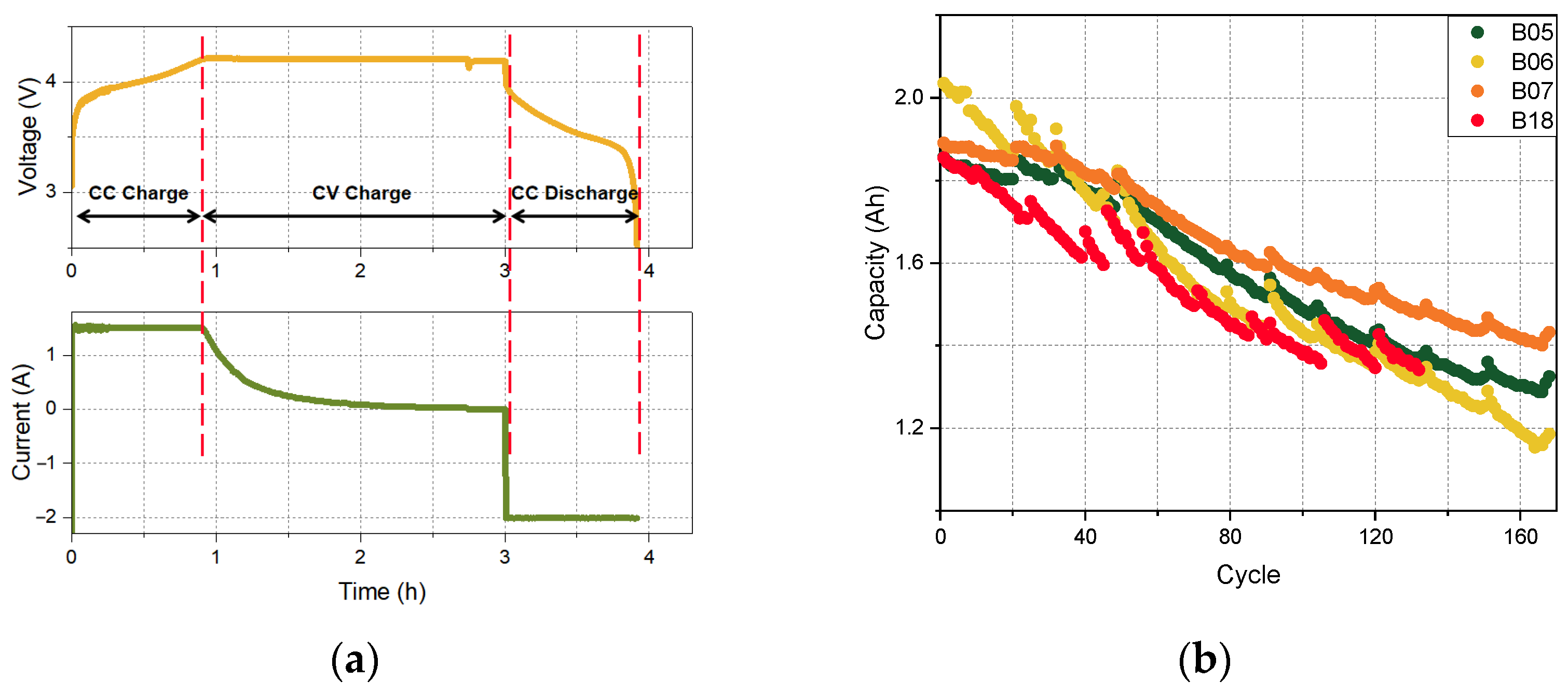
The experimental dataset in this paper is obtained from the NASA Ames Prognostics Center of Excellence, which consists of aging data for 18650 LIBs [26]. The four LIBs B05, B06, B07, and B18 are tested in standard charging and discharging processes under 25 Celsius. The experimental steps of a cycle are as follows and are shown in Figure 1a:
- Charging process: first, the voltage was raised to 4.2 V under a 1.5 A constant current (CC phase), and then kept charging at 4.2 V constant voltage until the charge current dropped to 20 mA (CV phase).
- Discharge process: the battery was discharged at a constant current of 2 A until the voltage of B05, B06, B07, and B18 dropped to the cutoff voltage of 2.7 V, 2.5 V, 2.2 V, and 2.5 V, respectively.
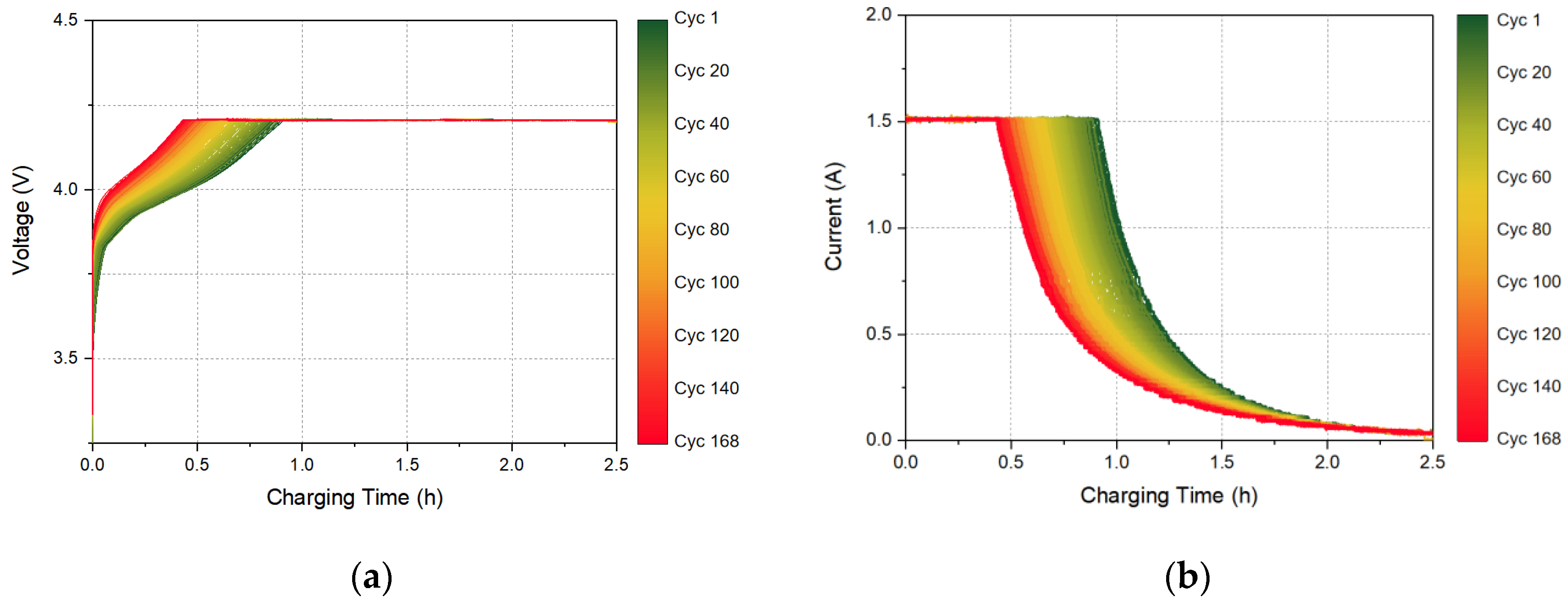
The experiments were halted when the battery capacity decayed to 70%. The tested charge life cycle number of B05, B06, B07, and B18 batteries are 168, 168, 168, and 132 cycles, respectively. The degradation tendencies of battery capacity under different cycle numbers are described in Figure 1b. In this paper, the charging process is selected to study the aging law of LIBs. Figure 2 illustrates the variations of voltage and current of B05 in the CC-CV charging as battery aging. In the CC charging phase, the duration shortens, and the voltage curve moves leftward as battery cycling, which shows the charging capacity in this phase is decreasing. In the CV charging phase, it presents an increasing duration, and the charging capacity showed an opposite trend as in the CC phase.
2.2. IC Curve and Smoothing Method
The IC curve indicates the change rate of capacity over the voltage evolution during the charging process as an efficient tool to study the variation in the electrochemical properties of LIBs. It has been proved that the batteries with different aging levels have a slight shift in charging voltage or current curve due to the big voltage plateaus during the low-rate cycle [27]. By calculating the derivative of the charging capacity to battery voltage, the IC curve analysis can convert the voltage plateaus into the intuitive and recognizable fluctuation on the IC curve, to detect a gentle change accurately during battery aging [28,29].
The intensity of reactions between electrodes is affected by battery aging during the charging process, where the difference is implicit in the voltage curve but can be reflected in the IC curve as inflection points or even peaks [30]. We can track the battery state and even predict the battery aging trajectory from the inflection points vanishing, decreasing, and shifting, since the slight capacity aging caused by battery degradation can be identified quantitatively by the IC curve [31].
Because the charging capacity is divided by the terminal voltage change within an equal time interval (ETI) and equal voltage interval (EVI) [32], the IC curve can be obtained as shown in Equations (1) and (2).
where QC and VC are the battery charging capacity and battery terminal voltage, respectively. iC and t are the current and the time in the CC charging phase, which can calculate the charging capacity in the ETI method. QC,2 − QC,1 is the charging capacity in the CV charging phase.
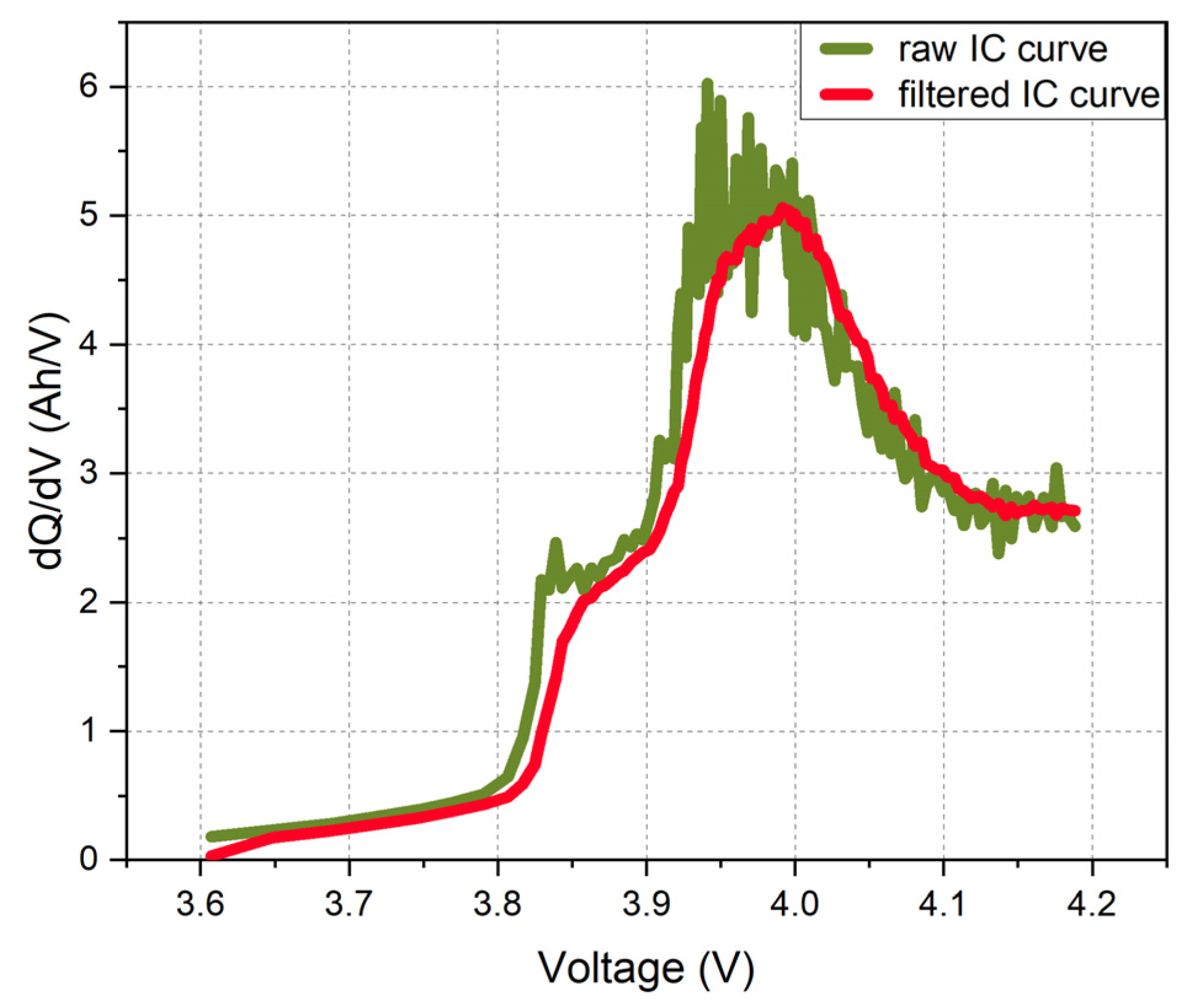
As shown in the green line in Figure 3, the curve calculated by Equation (1) as the sample is polluted by measurement noise owing to impact by the selected interval. If the interval is small, the IC curve will be noisy, and if the interval is large, the IC curve features will become indistinct [32]. It is challenging to catch useful shape features as the peak characteristic is not transparent. In this study, the Kalman filter (KF) is applied as a proper filtering algorithm to improve the curve smoothing.
Firstly, the evolution of x = ∆Q/∆V can be modeled as a random walk with additive Gaussian process noise ω and measurement noise υ, then the state equation and observation equation are as follows:
where yk represents the noise-polluted measurement of xk, uk is the external input of the system, ωk represents the measurement noise, and υk represents the process noise. Q and R are defined as the covariance of process noise and measurement noise, Kk is the Kalman gain, and Pk is the covariance of estimate value. Then, the filtering algorithm based on the nominal model of Equation (3) can be formulated as:
State and error covariance,
Process and measurement noise,
State and error covariance time update,
Kalman gain,
State and error covariance measurement update,
where uk is defined as zero due to no external input of the system, and the system state and system output are xk = (dQ/dV)k and yk = ∫icdt. We set x0 = 0 and P0 = 1. The red curve in Figure 3 is the filtered IC curve and the inflection points can be clearly identified. The smoothing method provides a basis for the further development of the HIs extraction.
2.3. HIs Extraction and Correlation Analysis
2.3.1. Aging Mechanism Based on IC Analysis
Battery aging is a certainty with corrosion and consumption in the internal material structure of the battery due to electrochemical as well as side reactions in the battery during cycling and storage [33]. According to the research of Ref. [34], the aging mechanisms for LIBs can be categorized into the two main degradation phases: linear degradation phase and accelerated degradation phase. In the linear degradation phase, the battery capacity declines under a linear trend, which is mainly caused by the loss of lithium inventory (LLI), including the formation of SEI film on the surface of the negative electrode, the dilution of electrolyte derived from the side reactions, lithium deposition, and other typical aging mechanisms [35]. In the accelerated degradation phase, the battery capacity is aggravated to decline, where the loss of active material (LAM) emerges as a major factor. The active material is physically damaged and decomposed by the chemical reaction, which affects the intensity of the electrochemical reaction and the transportation of lithium ions between electrodes. Moreover, the products generated by the LLI aging mode, and the polymer decomposed by the electrolyte and lithium deposition can accumulate and be attached to the active material, causing isolation between lithium ions and material as well as material breaking [36,37].
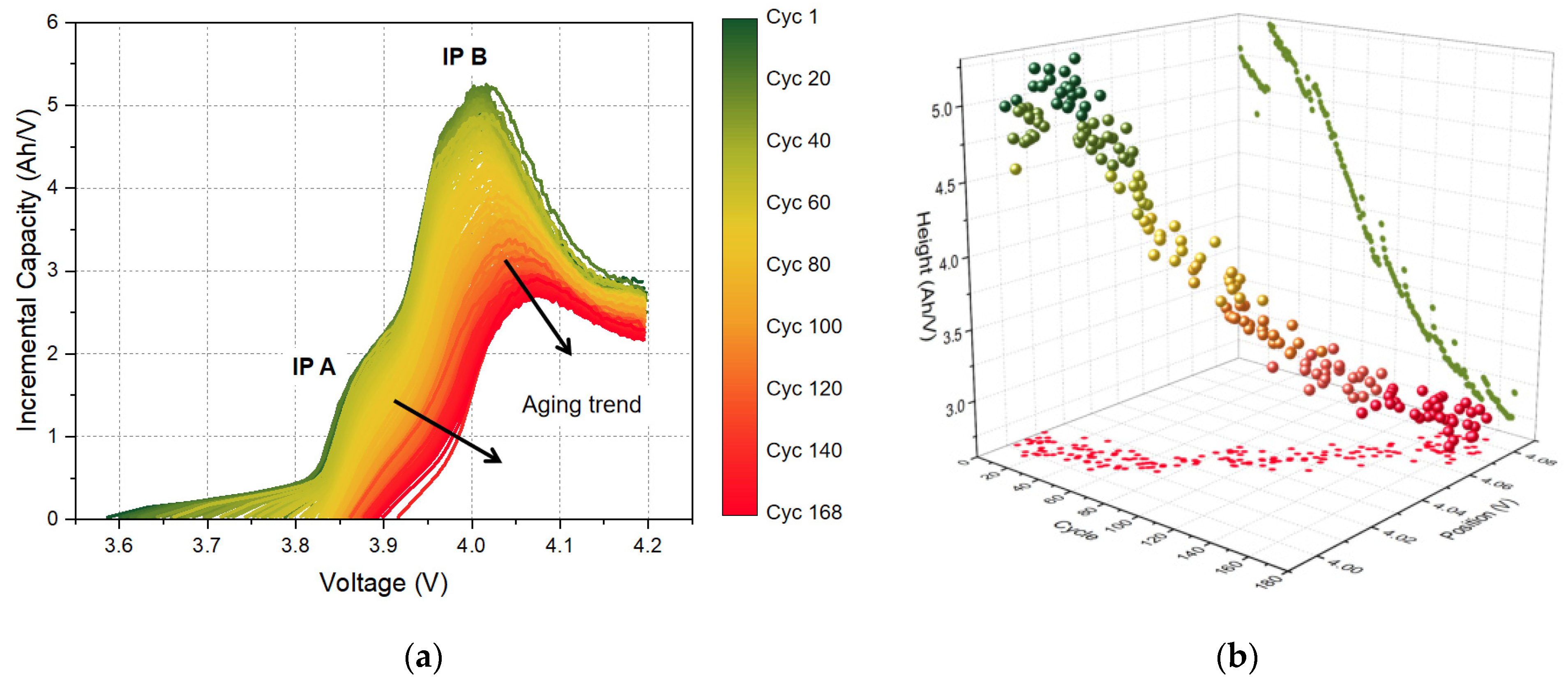
These aging modes are also distinguished in the IC curve. As depicted in Figure 4a, the IC curve in different charging cycles, B05 as the sample, displayed a clear rightward and lower trend along with two obvious inflection points (IP) on the curve, named IP A and IP B. Owe to discrepancy in LIBs internal characteristics, the intensity of inflection is variable. The IC curves of some batteries show slight inflection, and others are inflected into a peak. According to the previous research [32,38] on the degradation mode based on the IC curve feature, it is clear that in terms of LLI and LAM, the intensity of IP A and B will decrease and move toward the higher voltage section during battery cycling, just as Figure 4a. Conversely, IP A and B evolve in opposite trends, and the intensity of IP A is more influenced by LAM mode than LLI mode, and the intensity of IP B mainly depends on LLI mode. Furthermore, for the scenario of EV driving, the battery works in a linear degradation phase as the EOL is most defined as the range from 70% to 80%, so IP B can be more recommended to be the indicator containing aging information than IP A.
2.3.2. Extraction of HIs
In the driving scenario, the battery cannot be discharged under constant current conditions as in the laboratory, which depends on the unpredictable load demand during driving. It is hard to calculate the capacity through the Ampere hour integral method and capture characteristic aging parameters by the discharging curves. Conversely, the charging process is constant due to the regular charging strategy, where the slight shift can be identified. In this study, the IC curve is calculated through the ETI method for the CC charging process as Section 2.2, using charging voltage and CC charging current data. The height of IP B as shape feature characteristic of IC curve and corresponding voltage standing for inflection point position are selected as two HIs for battery RUL prediction, named F1 and F2. The evolution trends of the two HIs with different cycles, B05 still as a sample, are illustrated in Figure 4b.
Compared to laboratory conditions, the charging process is usually incomplete with commercial chargers due to the driver’s habit, but the charging curve still retains the shape characteristics of the CC-CV phase, especially the complete curve shape in the CV charging phase, although the different depth of discharge (DOD) in the different cycle may influence battery charging. Owe to the above-mentioned reasons, the HIs of the CV phase can be extracted directly instead of conversion by the IC method, which ensures the characteristic undistorted transmission in practice.
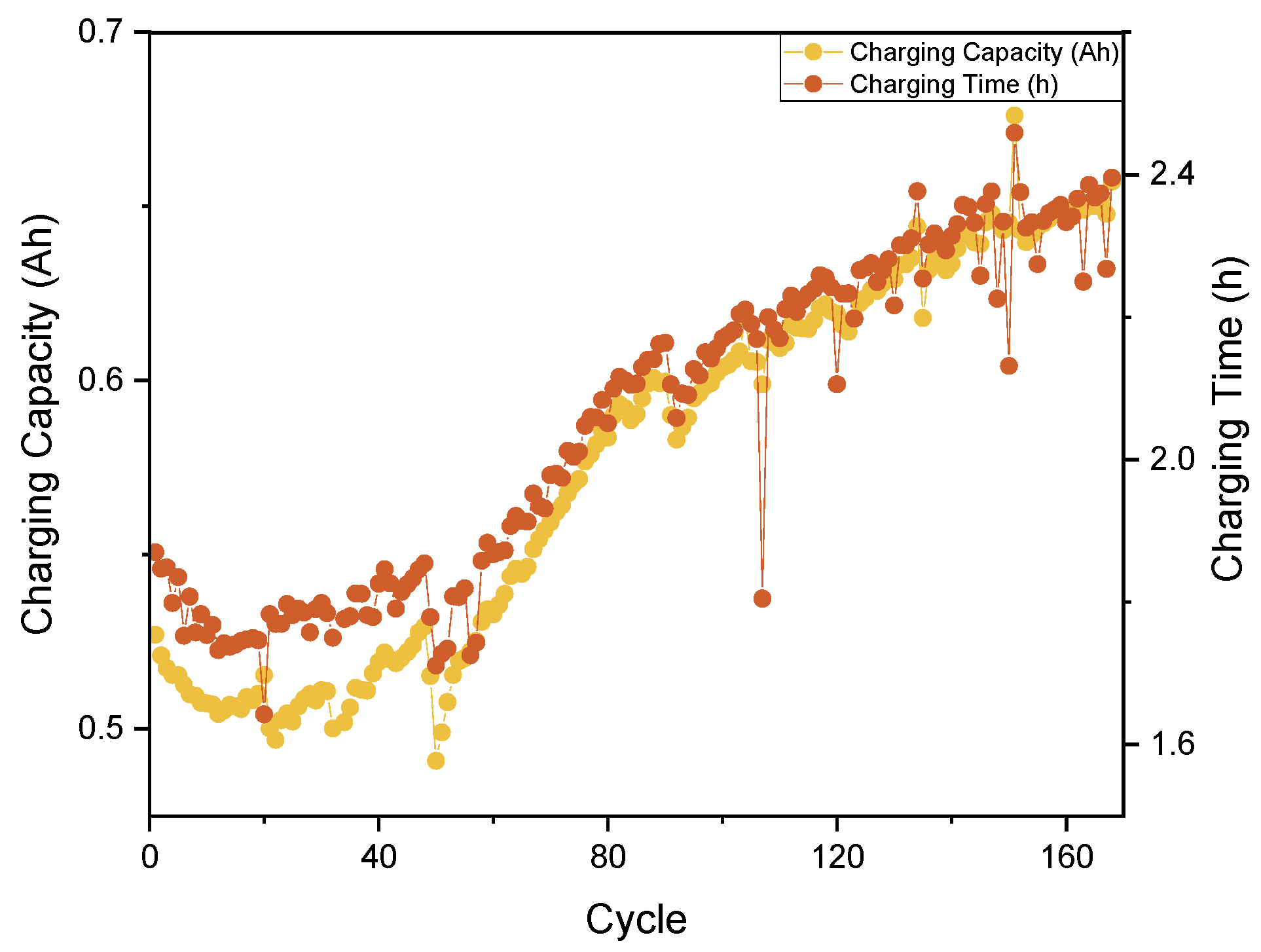
Similar to the CC phase, there are also some regular shifts like indicators for battery aging in the CV phase as Figure 2 depicted. According to voltage balance Equation (5), because of the increase of polarization voltage UP and ohmic internal resistance during degradation, UT reaches a cut-off voltage earlier, and the charging process switches to the CV phase in a shorter time, which can lead to different charging time and charging capacity in every cycle as shown in Figure 5.
where UT is terminal voltage, UOCV is open-circuit voltage, UP is polarization voltage, and UR is ohmic internal resistance voltage.
Hence, the charging capacity of the CV charging phase is chosen as another HI F3 to characterize the capacity degradation, and it can be formulated by the Ampere hour integral method as:
where ICV is the current in the CV charging phase, t1 and t2 are the start-stop time of the CV charging phase.
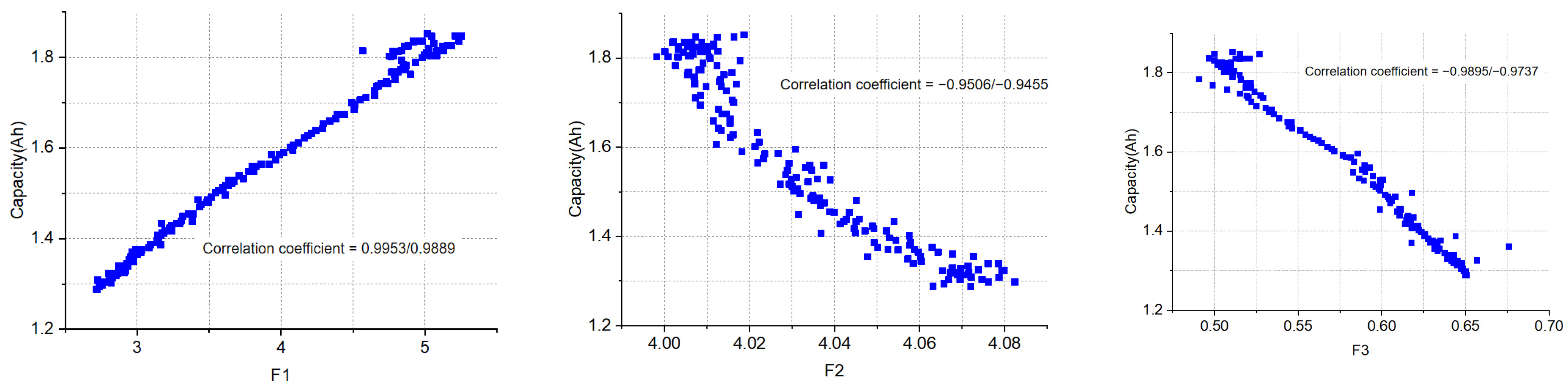
In conclusion, the height of IP B in the IC curve and corresponding voltage standing for the position of inflection point as F1 and F2 in the CC charging phase and the charging capacity of the CV charging phase as F3 are selected as HIs for battery RUL prediction. F1 and F2 can highlight the slight shifts in the voltage plateau phase in the charging process, and F3 represents the charging condition and polarization of the battery. All the HIs reflect the characteristics of the entire battery charging process.
2.3.3. Correlation Analysis of HIs
To further explore the relationship among the three HIs and probe whether all of them can express the change in the battery capacity, the interaction between the HIs and capacity is analyzed by the Pearson correlation and the Spearman correlation. The analysis results are displayed in Table 1 and Figure 6. As the correlation coefficient of F1 (Height of IP B), F3 (Charging capacity of CV phase) is close to 1, and the absolute value of F2 (Position of IP B) also exceeds 0.94, the correlation of model input parameters is quite significant.
3. Online Estimation Based on AutoML
3.1. Description of AutoML Model
We established a novel model based on AutoML, automatically customizing the forecasting pipeline, which consists of data pre-processing, feature engineering, and automatic modeling with less human intervention and trial error manually, covering the complete actions from processing the input data to the deployment of the model.
Each step of data pre-processing, including data cleaning, data augmentation, and data coding, can search the configuration space automatically by some optimization algorithm, such as reinforcement learning and grid search. The pre-processing contributes to input data without polluted noise, avoiding over-fitting of model training and enhancing model robustness. Data pre-processing also involves normalizing, through which the available data can eliminate the effect caused by the different ranges of value in the learning phase. We use the Min-max normalization to map the range of feature S into [a, b] as follows:
where x and x’ are the value and the transformed value of the feature S.
Feature engineering is to automatically construct features from the data so that subsequent learning models can have good performance, with the segment of feature extraction, feature selection, and feature enhancement. It ensures that the features can exclude the redundant variable and be extracted in an appropriate dimensionality for the feature space.
AutoML aims to solve the so-called CASH problem, the short for combined algorithm selection and hyperparameters optimization [39]. This is essentially the task of selecting or combining the appropriate model for the dataset at hand automatically, along with the various hyperparameters tuned properly in every segment of the pipeline.
The model performance mostly depends on a set of hyperparameters that make up the algorithm. Hyperparameters are tuned specifically to that dataset, with some techniques like Regression Trees, and Gaussian Processes [40]. Bayesian optimization has been applied as a successful candidate for hyperparameter tuning, which fits a probabilistic model to capture the relationship between hyperparameters’ setting and their measured performance. Then, the most promising hyperparameter setting is selected and evaluated, as well as updated in the model with the result, finishing an entire iteration [41].
The meta-learning approach is complementary to Bayesian optimization for optimizing a model architecture, which is employed to obtain promising configurations to warmstart Bayesian Optimization. Each model trained on data contributes to the configuration space of hyperparameters cross datasets, even if a model performed poorly. The area of meta-learning [42] follows this common strategy that human experts screen known models by reasoning about the performance of learning algorithms and searching with configuration space. Therefore, meta-learning is applied to select instantiations of the given model frameworks, which tend to perform well on a new dataset, from the knowledge of previous tasks [43]. To characterize explicitly discrepancy in dataset repositories, meta-features are introduced as the searching targets and data depiction, denoting some dimensions, such as Statistical meta-features, PCA meta-features, information-theoretic meta-feature, etc. [43]. They comprise the attributes of each dataset and the parameters of the computing model, such as neural network training weights. More precisely, the meta-learning approach works as follows:
Step 1 For each machine learning dataset in a dataset repository, we evaluated a set of meta-features and used Bayesian optimization to determine and store an instantiation of the given ML framework with strong empirical performance for that dataset.
Step 2 Then, for the given new dataset, we compute its meta-features, sort out all datasets by distance metric among them in meta-feature space and select the stored ML architecture instantiations for the limited nearest datasets for evaluation before starting Bayesian optimization with their results.
In this study, we used Auto-sklearn architecture combined with a meta-learning approach and Bayesian optimization, which is a robust new AutoML system based on scikit-learn, comprising 15 classifiers, 14 feature preprocessing methods, and 4 data preprocessing methods, giving rise to a structured hypothesis space with 110 hyperparameters. The architecture improves the existing AutoML methods by automatically taking into account past performance on similar datasets, and by constructing ensembles from the models evaluated during the optimization [44]. EarlyStopping is used as callbacks to prevent overfitting, which can stop training when the loss did not decrease anymore in each epoch. The network training weights in the current epoch are the final training results.
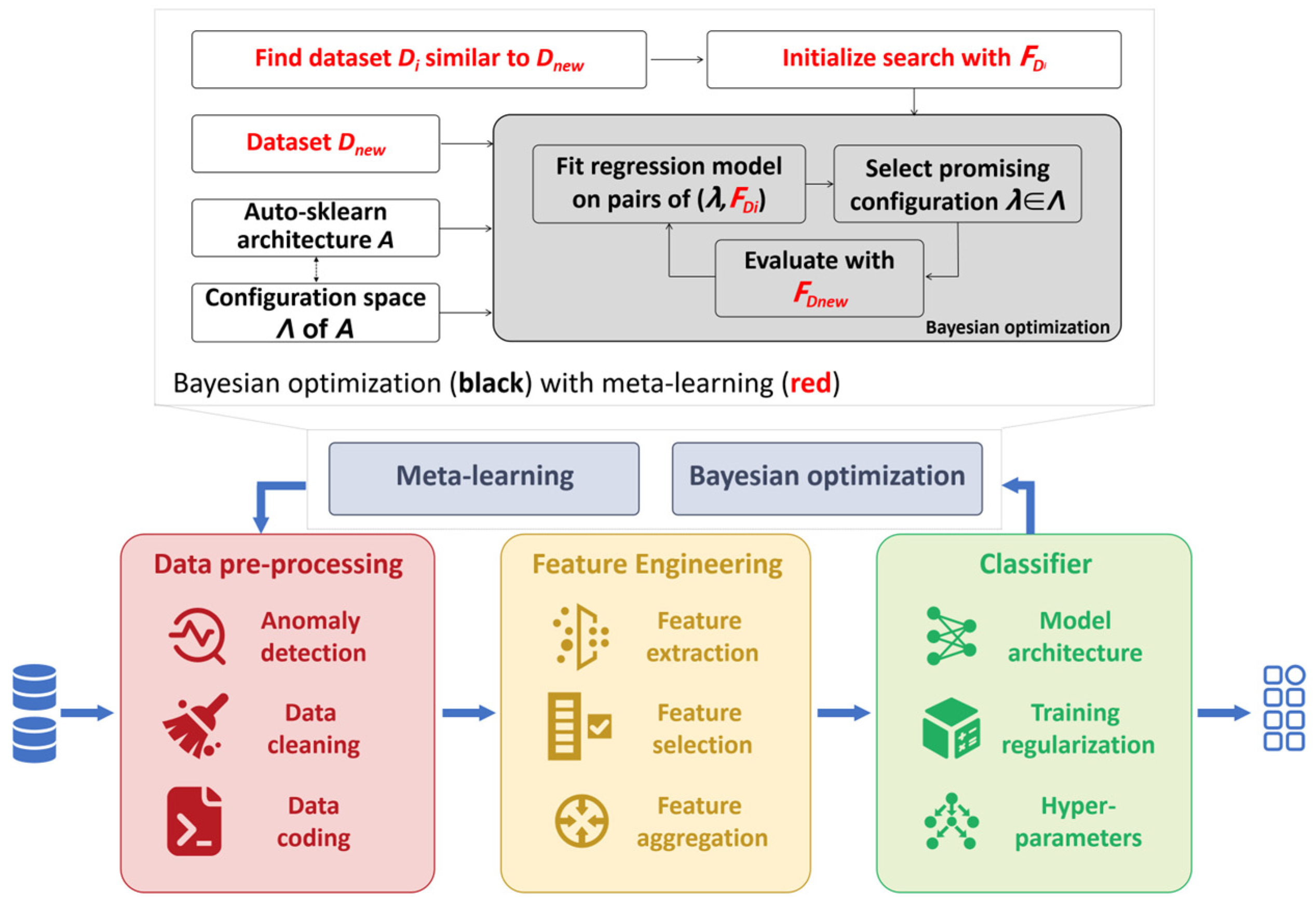
The flow chart for pipelined-based AutoML is show in Figure 7. Configuration space Λ is built up based on the algorithm repository A in Auto-sklearn architecture, which comprises the hyperparameters controlling each algorithm. Meta-learning searches the existing dataset Di similar to the new dataset Dnew in the dataset repository, in which similarity is defined by a distance between two datasets based on meta-features, and initializes a search with the meta-feature FDi. For each dataset, meta-features are only computed on the training set. In contrast to human domain experts, Bayesian Optimization does not use knowledge from previous runs on different datasets and uses the matched FDi to obtain promising configurations λ, in which the model is evaluated with the new meta-feature FDnew based. The Bayesian Optimization with meta-learning finishes the pipeline including data pre-processing, feature engineering, and classifier selection.
3.2. Framework of RUL Prediction Method
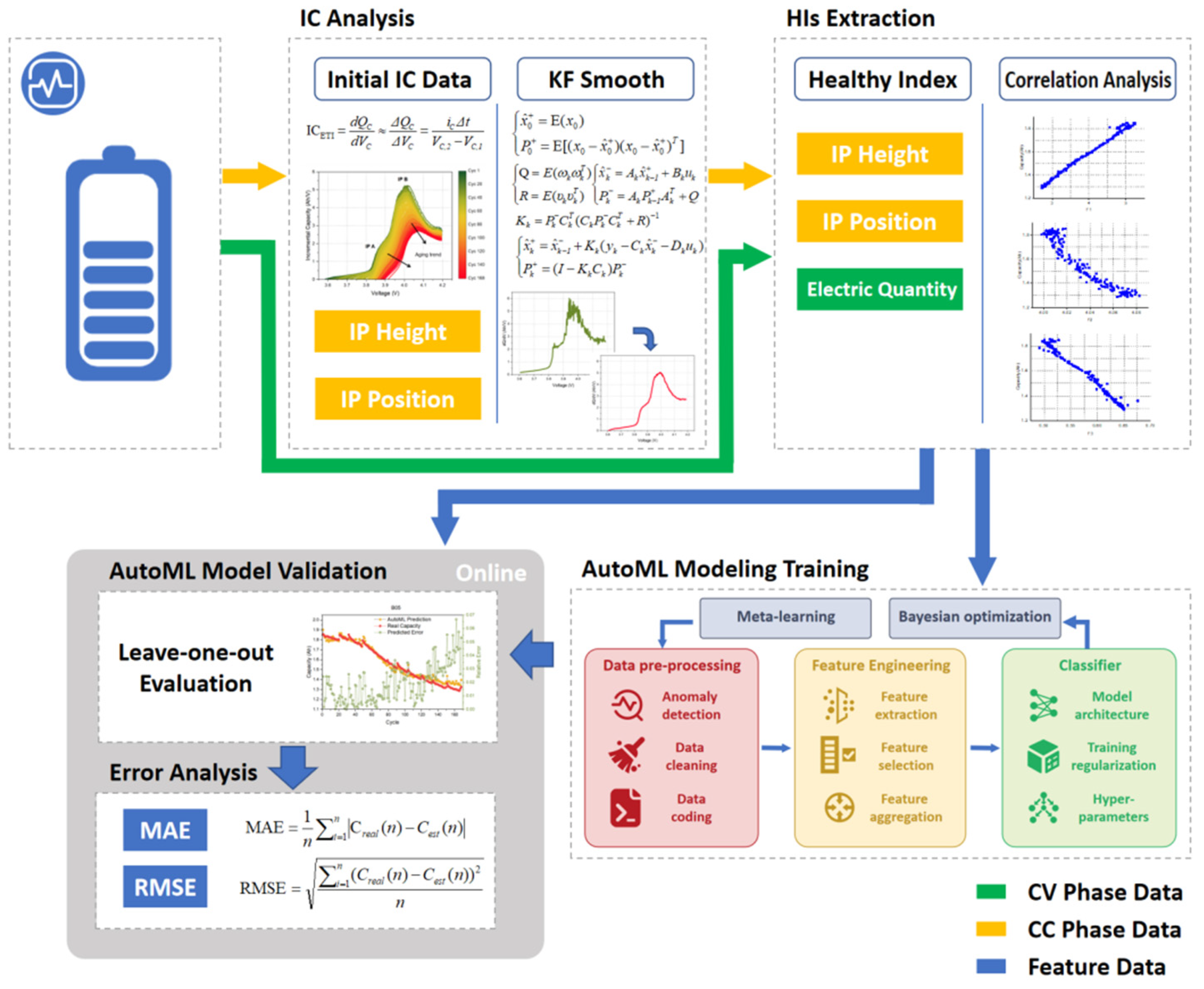
The integrated framework for the life prediction approach is described in Figure 8 and divided into offline training and online prediction. In the offline stage, first, the IC curve is calculated in the CC charging phase, in which the two HIs that inflection point height and position are extracted, with the curve smoothing method derived from the KF algorithm. Combined with the charging capacity in the CV phase of every cycle, all three HIs effectively characterize the battery aging of the entire charging process. Then, a novel AutoML model is established with Auto-sklearn architecture, to realize the automatic design of the pipeline. The model hyperparameters are tuned and the search is optimized in the training stage. In the online stage, the extracted three features are directly applied to predict the battery RUL based on the trained AutoML model.
4. Results and Discussion
4.1. Evaluation Criteria
In this study, root mean square error (RMSE) and mean absolute error (MAE) indexes are applied to evaluate the performance of the prediction method. The formulae for calculating are as follows:
where n is the number of cycles, Creal is the real capacity, and Cprd is the predicted capacity.
In most experiment settings in data-driven methods, the training set and validation set are usually divided on the same single battery, which can implement the online prediction. In the driving scenario, unlike in the bench test, the BMS cannot predict online capacity without the first 60% to 80% battery running data, so the goal of online prediction for the entire battery aging cycle is hard to achieve. To tackle this, we use the leave-one-out evaluation as Chen et al. [45] applied to evaluate their model: one battery is sampled for validation, and the other three batteries are used for training. A total of four trials are conducted and hyperparameters of the model as well as the average evaluating index over all batteries are determined.
4.2. Prediction Results and Analysis
As the framework showed in Figure 8, the HIs F1, F2, and F3 calculated by raw voltage and current data are used as input of the AutoML model, and the training set and validation set are divided by leave-one-out evaluation.
By means of searching and evaluating, the three methods, poly, rbf, and sigmoid, are used for feature preprocessing, and the five classifiers are selected in the AutoML model, and the classifiers’ type and ensembled weight are listed in Table 2. In Table 3 we show the hyperparameters used in this study.
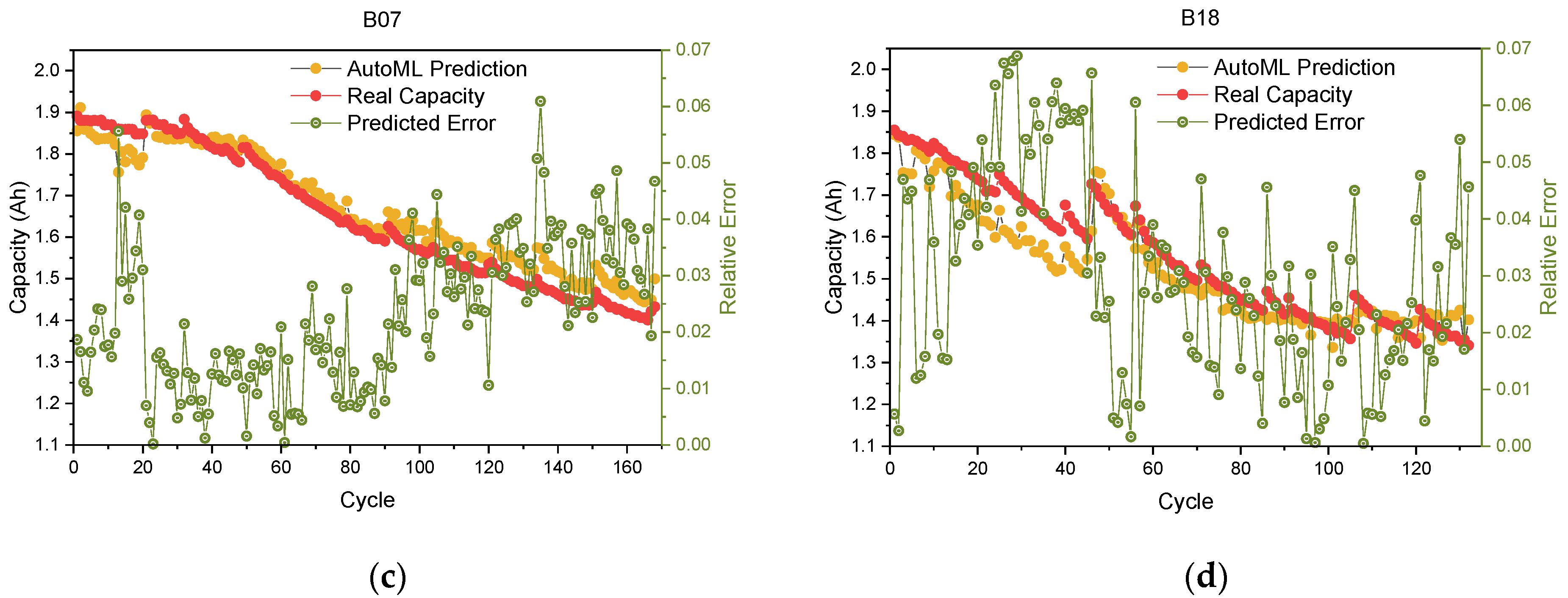
The capacity prediction and relative error of B05, B06, B07, and B18 are depicted in Figure 9. The red predicted capacity curve approximates the yellow real capacity curve with most prediction errors controlled within 7% in the validation of four batteries, indicating high accuracy and robustness.
Compared to the RMSE value in Table 4, the lowest prediction accuracy among the four batteries is B18. Although it is not as good as other batteries, the MAE of B18 is 0.0479, indicating the test accuracy rate reached more than 95%. According to the development requirements of batteries in EVs, the fault threshold is set to 80% of initial capacity, and the life value can also be predicted. The predicted error is 1 and 8 cycles for B06 and B18 respectively. All of the above illustrates that the proposed online prediction method has high accuracy and reliability.
We conducted the same training and validation for NASA’s data and average evaluation index as in Ref. [45], so we can perform a valid benchmark comparison. Table 5 summarizes the RUL prediction results from various methods, and it is obvious that the proposed method achieves a better performance than other methods, which is presented in Ref. [45]. It is obvious that the prediction based on AutoML is more accurate using the same data set and training method, with the MAE increased by 52.8% and RMSE increased by 48.3% than DeTransformer.
5. Conclusions
In this study, according to our knowledge, we are the first to propose the AutoML model applied in the RUL prediction of LIBs, with the HIs extracted by IC analysis. A smoothing IC curve based on the KF algorithm is employed for HIs extraction and three HIs have been verified to characterize the aging phenomenon in the entire charging process including the CC and CV phases. We proposed a prediction method based on AutoML running in the Auto-sklearn architecture, which can customize the pipeline for specific datasets automatically, overcoming the problem of redundant model information and high computational cost. Then the experiment on NASA’s LIBs cycle life dataset verifies the accuracy and robustness. As a next step, we plan to keep on further studies on neural networks in the AutoML model, using neural architecture search to improve pipeline, as well as investigating effective dimensionality optimization techniques for the HIs extraction by IC analysis.
Author Contributions
Conceptualization, C.L. and Z.Z.; methodology, C.L. and D.Q.; software, C.L. and Y.L.; validation, C.L. and Y.L.; formal analysis, C.L. and D.Q.; investigation, C.L.; resources, C.L.; data curation, C.L. and D.Q.; writing—original draft preparation, C.L.; writing—review and editing, C.L.; visualization, C.L.; supervision, Z.Z. and X.L.; project administration, C.L. and S.W.; funding acquisition, Z.Z. and X.L. All authors have read and agreed to the published version of the manuscript.
Funding
This research was funded by the National Natural Science Foundation of China, grant number 51977131.
Institutional Review Board Statement
Not applicable.
Informed Consent Statement
Not applicable.
Data Availability Statement
Not applicable.
Conflicts of Interest
The authors declare no conflict of interest.
References
- Liu, K. Data-driven health estimation and lifetime prediction of lithium-ion batteries: A review. Renew. Sustain. Energy Rev. 2019, 113, 109254. [Google Scholar] [CrossRef]
- Tian, H.; Qin, P.; Li, K.; Zhao, Z. A review of the state of health for lithium-ion batteries: Research status and suggestions. J. Clean. Prod. 2020, 261, 120813. [Google Scholar] [CrossRef]
- Lai, X.; Chen, Q.; Tang, X.; Zhou, Y.; Gao, F.; Guo, Y.; Bhagat, R.; Zheng, Y. Critical review of life cycle assessment of lithium-ion batteries for electric vehicles: A lifespan perspective. eTransportation 2022, 12, 100169. [Google Scholar] [CrossRef]
- Liao, Z.; Gai, N.; Stansby, P.K.; Li, G. Linear non-causal optimal control of an attenuator type wave energy converter M4. IEEE Trans. Sustain. Energy 2020, 11, 1278–1286. [Google Scholar] [CrossRef] [Green Version]
- Xu, X.; Chen, N. A state-space-based prognostics model for lithium-ion battery degradation. Reliab. Eng. Syst. Saf. 2017, 159, 47–57. [Google Scholar] [CrossRef]
- Miao, Q.; Xie, L.; Cui, H.; Liang, W.; Pecht, M.G. Remaining useful life prediction of lithium-ion battery with unscented particle filter technique. Microelectron. Reliab. 2013, 53, 805–810. [Google Scholar] [CrossRef]
- Jin, X.; Lian, X.; Su, T.; Shi, Y.; Miao, B. Closed-loop estimation for randomly sampled measurements in target tracking system. Math. Probl. Eng. 2014, 2014, 315908. [Google Scholar]
- Richardson, R.R.; Osborne, M.A.; Howey, D.A. Gaussian process regression for forecasting battery state of health. J. Power Sources 2017, 357, 209–219. [Google Scholar] [CrossRef]
- Yun, Z.; Qin, W.; Shi, W.; Ping, P. State-of-health prediction for lithium-ion batteries based on a novel hybrid approach. Energies 2020, 13, 4858. [Google Scholar] [CrossRef]
- Zhang, S.; Zhai, B.; Guo, X.; Wang, K.; Peng, N.; Zhang, X. Synchronous estimation of state of health and remaining useful lifetime for lithium-ion battery using the incremental capacity and artificial neural networks. J. Energy Storage 2019, 26, 100951.1–100951.12. [Google Scholar] [CrossRef]
- Sun, T.; Wang, S.; Jiang, S.; Xu, B.; Han, X.; Lai, X.K.; Zheng, Y. A cloud-edge collaborative strategy for capacity prognostic of lithium-ion batteries based on dynamic weight allocation and machine learning. Energy 2022, 239, 122185. [Google Scholar] [CrossRef]
- Dong, D.; Li, X.Y.; Sun, F.Q. Life prediction of jet engines based on LSTM-recurrent neural networks. In Proceedings of the 2017 Prognostics and System Health Management Conference (PHM-Harbin), Harbin, China, 9–12 July 2017. [Google Scholar]
- Zraibi, B.; Okar, C.; Chaoui, H.; Mansouri, M. Remaining useful life assessment for lithium-ion batteries using CNN-LSTM-DNN hybrid method. IEEE Trans. Veh. Technol. 2021, 70, 4252–4261. [Google Scholar] [CrossRef]
- Wang, F.; Zemenu, E.A.; Tseng, C.; Chou, J. A hybrid method for online cycle life prediction of lithium-ion batteries. Int. J. Energy Res. 2022, 46, 9080–9096. [Google Scholar] [CrossRef]
- Tang, T.; Yuan, H. A hybrid approach based on decomposition algorithm and neural network for remaining useful life prediction of lithium-ion battery. Reliab. Eng. Syst. Saf. 2022, 217, 108082. [Google Scholar] [CrossRef]
- Yao, Q.; Wang, M.; Escalante, H.J.; Guyon, I.; Hu, Y.; Li, Y.; Tu, W.; Yang, Q.; Yu, Y. Taking human out of learning applications: A survey on automated machine learning. arXiv 2018, arXiv:1810.13306. [Google Scholar]
- Gomathi, S.; Kohli, R.; Soni, M.; Dhiman, G.; Nair, R. Pattern analysis: Predicting COVID-19 pandemic in India using AutoML. World J. Eng. 2022, 19, 21–28. [Google Scholar] [CrossRef]
- Zeng, Y.; Zhang, J. A machine learning model for detecting invasive ductal carcinoma with google cloud AutoML vision. Comput. Biol. Med. 2020, 122, 103861. [Google Scholar] [CrossRef]
- Drori, I.; Liu, L.; Nian, Y.; Koorathota, S.C.; Li, J.; Moretti, A.K.; Freire, J.; Udell, M. AutoML using metadata language embeddings. arXiv 2019, arXiv:1910.03698. [Google Scholar]
- Galanopoulos, A.; Ayala-Romero, J.A.; Leith, D.J.; Iosifidis, G. AutoML for video analytics with edge computing. In Proceedings of the IEEE INFOCOM 2021-IEEE Conference on Computer Communications, Vancouver, BC, Canada, 10–13 May 2021. [Google Scholar]
- Kefalas, M.; Baratchi, M.; Apostolidis, A.; Herik, D.V.; Bäck, T. Automated machine learning for remaining useful life estimation of aircraft engines. In Proceedings of the 2021 IEEE International Conference on Prognostics and Health Management (ICPHM), Detroit, MI, USA, 7–9 June 2021. [Google Scholar]
- Tornede, T.; Tornede, A.; Wever, M.; Hüllermeier, E. Coevolution of remaining useful lifetime estimation pipelines for automated predictive maintenance. In Proceedings of the Genetic and Evolutionary Computation Conference, Lille, France, 10–14 July 2021. [Google Scholar]
- Tornede, T.; Tornede, A.; Wever, M.; Mohr, F.; Hüllermeier, E. AutoML for predictive maintenance: One tool to RUL them all. In Proceedings of the IoT Streams for Data-Driven Predictive Maintenance and IoT, Edge, and Mobile for Embedded Machine Learning, Ghent, Belgium, 14–18 September 2020. [Google Scholar]
- Chao, M.A.; Kulkarni, C.S.; Goebel, K.F.; Fink, O. Aircraft engine run-to-failure dataset under real flight conditions for prognostics and diagnostics. Data 2021, 6, 5. [Google Scholar] [CrossRef]
- Le, T.T.; Fu, W.; Moore, J. Scaling tree-based automated machine learning to biomedical big data with a feature set selector. Bioinformatics 2020, 36, 250–256. [Google Scholar] [CrossRef] [Green Version]
- Goebel, K.; Saha, B.; Saxena, A.; Celaya, J.R.; Christophersen, J. Prognostics in battery health management. IEEE Instrum. Meas. Mag. 2008, 11, 33–40. [Google Scholar] [CrossRef]
- Qiao, D.; Wei, X.; Fan, W.; Jiang, B.; Lai, X.; Zheng, Y.; Tang, X.; Dai, H. Toward safe carbon–neutral transportation: Battery internal short circuit diagnosis based on cloud data for electric vehicles. Appl. Energy 2022, 317, 119168. [Google Scholar] [CrossRef]
- Feng, X.; Li, J.; Ouyang, M.; Lu, L.; Li, J.; He, X. Using probability density function to evaluate the state of health of lithium-ion batteries. J. Power Sources 2013, 232, 209–218. [Google Scholar] [CrossRef]
- Weng, C.; Jing, S.; Peng, H. A unified open-circuit-voltage model of lithium-ion batteries for state-of-charge estimation and state-of-health monitoring. J. Power Sources 2014, 258, 228–237. [Google Scholar] [CrossRef]
- Xue, N.; Sun, B.; Bai, K.; Han, Z.; Li, N. Different state of charge range cycle degradation mechanism of composite material lithium-ion batteries based on incremental capacity analysis. Trans. China Electrotech. Soc. 2017, 32, 145–152. [Google Scholar]
- Han, X.B. Study on Li-Ion Battery Mechanism Model and State Estimation for Electric Vehicles. Ph.D. Dissertation, Tsinghua University, Beijing, China, 2014. [Google Scholar]
- Qiao, D.; Wang, X.; Lai, X.; Zheng, Y.; Wei, X.; Dai, H. Online quantitative diagnosis of internal short circuit for lithium-ion batteries using incremental capacity method. Energy 2022, 243, 123082. [Google Scholar] [CrossRef]
- Vetter, J.; Novák, P.; Wagner, M.R.; Veit, C.; Hammouche, A. Ageing mechanisms in lithium-ion batteries. J. Power Sources 2005, 147, 269–281. [Google Scholar] [CrossRef]
- Dubarry, M.; Berecibar, M.; Devie, A.; Anseán, D.; Omar, N.; Villarreal, I. State of health battery estimator enabling degradation diagnosis: Model and algorithm description. J. Power Sources 2017, 360, 59–69. [Google Scholar] [CrossRef]
- Bloom, I.D.; Cole, B.W.; Sohn, J.; Jones, S.A.; Polzin, E.G.; Battaglia, V.S.; Henriksen, G.L.; Motloch, C.G.; Richardson, R.A.; Unkelhaeuser, T.; et al. An accelerated calendar and cycle life study of Li-ion cells. J. Power Sources 2001, 101, 238–247. [Google Scholar] [CrossRef]
- Dubarry, M.; Truchot, C.; Liaw, B.Y. Synthesize battery degradation modes via a diagnostic and prognostic model. J. Power Sources 2012, 219, 204–216. [Google Scholar] [CrossRef]
- Anseán, D.; Dubarry, M.; Devie, A.; Liaw, B.Y.; Garcia, V.; Viera, J.C.; González, M. Fast charging technique for high power LiFePO4 batteries: A mechanistic analysis of aging. J. Power Sources 2016, 321, 201–209. [Google Scholar] [CrossRef]
- Han, X.; Ouyang, M.; Lu, L.; Li, J.; Zheng, Y.; Li, Z. A comparative study of commercial lithium ion battery cycle life in electrical vehicle: Aging mechanism identification. J. Power Sources 2014, 251, 38–54. [Google Scholar] [CrossRef]
- Thornton, C.; Hutter, F.; Hoos, H.H.; Leyton-Brown, K. Auto-weka: Combined selection and hyperparameter optimization of classification algorithms. In Proceedings of the 19th ACM SIGKDD International Conference on Knowledge Discovery and Data Mining (KDD ‘13), Chicago, IL, USA, 11–14 August 2013. [Google Scholar]
- Nagarajah, T.; Poravi, G. A review on automated machine learning (AutoML) Systems. In Proceedings of the 2019 IEEE 5th International Conference for Convergence in Technology (I2CT), Bombay, India, 29–31 March 2019. [Google Scholar]
- Brochu, E.; Cora, V.M.; Freitas, N.D. A tutorial on Bayesian optimization of expensive cost functions, with application to active user modeling and hierarchical reinforcement learning. arXiv 2010, arXiv:1012.2599. [Google Scholar]
- Hodgson, J. Metalearning: Applications to data mining. Comput. Rev. 2010, 51, 217–218. [Google Scholar]
- Feurer, M.; Springenberg, J.T.; Hutter, F. Initializing Bayesian hyperparameter optimization via meta-learning. In Proceedings of the Twenty-Ninth AAAI Conference on Artificial Intelligence (AAAI-15), Austin, TX, USA, 25–30 January 2015. [Google Scholar]
- Feurer, M.; Klein, A.; Eggensperger, K.; Springenberg, J.T.; Hutter, F. Automated Machine Learning, 1st ed.; Springer: Cham, Switzerland, 2019; pp. 113–134. [Google Scholar]
- Chen, D.; Hong, W.; Zhou, X. Transformer network for remaining useful life prediction of lithium-ion batteries. IEEE Access 2022, 10, 19621–19628. [Google Scholar] [CrossRef]
Figure 1.
The experimental steps and capacity degradation profiles: (a) The voltage and current in a test cycle; (b) Capacity aging trends of the four batteries.
Figure 1.
The experimental steps and capacity degradation profiles: (a) The voltage and current in a test cycle; (b) Capacity aging trends of the four batteries.

Figure 2.
The variations of voltage and current of B05 in the CC-CV charging: (a) Charge voltage; (b) Charge current.
Figure 2.
The variations of voltage and current of B05 in the CC-CV charging: (a) Charge voltage; (b) Charge current.

Figure 3.
Smoothing results of IC curve.

Figure 4.
IC curve and HIs of B05 in different charging cycles: (a) IC curve; (b) Height and position of IP B as two HIs.
Figure 4.
IC curve and HIs of B05 in different charging cycles: (a) IC curve; (b) Height and position of IP B as two HIs.

Figure 5.
The charging time and capacity profiles of B05 in the CV phase in every cycle.

Figure 6.
Relationship of HIs and the reference capacity of B05.

Figure 7.
Flow chart for pipeline-based AutoML combined with meta-learning and Bayesian optimization.
Figure 7.
Flow chart for pipeline-based AutoML combined with meta-learning and Bayesian optimization.

Figure 8.
Framework of RUL prediction based AutoML.

Figure 9.
Capacity prediction results and errors of (a) B05, (b) B06, (c) B07, and (d) B18.


Table 1.
Results of correlation analysis of three HIs.
| HIs | Pearson Correlation | Spearman Correlation |
|---|---|---|
| F1 | 0.9953 | 0.9889 |
| F2 | −0.9506 | −0.9455 |
| F3 | −0.9895 | −0.9737 |
Table 2.
The classifiers type and ensembled weight in the AutoML model.
| Rank | Classifier Type | Ensembled Weight |
|---|---|---|
| 1 | Gaussian_process | 0.50 |
| 2 | K_nearest_neighbors | 0.32 |
| 3 | Gradient_boosting | 0.08 |
| 4 | Ard_regression | 0.08 |
| 5 | Liblinear_svr | 0.02 |
Table 3.
Hyperparameters used in verification.
| Hyperparameters | Data Type | Value Range |
|---|---|---|
| Initial configurations via meta-learning | int | 25 |
| Ensemble size | int | 50 |
| Max reserved models | int | 50 |
| batch size of training data | int | 64 |
| Number of training epochs | int | 200 |
| Resampling strategy | cat | Holdout |
| Model training optimizer | cat | SGD |
Table 4.
Prediction results of four batteries.
| B05 | B06 | B07 | B18 | |
|---|---|---|---|---|
| MAE | 0.0283 | 0.0221 | 0.0361 | 0.0479 |
| RMSE | 0.0337 | 0.0340 | 0.0407 | 0.0573 |
Table 5.
Comparison of prediction results of AutoML with other ML methods.
| MLP | RNN | LSTM | GRU | Daul-LSTM | DeTransformer | AutoML | |
|---|---|---|---|---|---|---|---|
| MAE | 0.1379 | 0.0749 | 0.0829 | 0.0806 | 0.0815 | 0.0713 | 0.0336 |
| RMSE | 0.1541 | 0.0848 | 0.0905 | 0.0921 | 0.0879 | 0.0802 | 0.0414 |
Publisher’s Note: MDPI stays neutral with regard to jurisdictional claims in published maps and institutional affiliations. |
© 2022 by the authors. Licensee MDPI, Basel, Switzerland. This article is an open access article distributed under the terms and conditions of the Creative Commons Attribution (CC BY) license (https://creativecommons.org/licenses/by/4.0/).
Share and Cite
MDPI and ACS Style
Luo, C.; Zhang, Z.; Qiao, D.; Lai, X.; Li, Y.; Wang, S. Life Prediction under Charging Process of Lithium-Ion Batteries Based on AutoML. Energies 2022, 15, 4594. https://0-doi-org.brum.beds.ac.uk/10.3390/en15134594
AMA Style
Luo C, Zhang Z, Qiao D, Lai X, Li Y, Wang S. Life Prediction under Charging Process of Lithium-Ion Batteries Based on AutoML. Energies. 2022; 15(13):4594. https://0-doi-org.brum.beds.ac.uk/10.3390/en15134594
Chicago/Turabian StyleLuo, Chenqiang, Zhendong Zhang, Dongdong Qiao, Xin Lai, Yongying Li, and Shunli Wang. 2022. "Life Prediction under Charging Process of Lithium-Ion Batteries Based on AutoML" Energies 15, no. 13: 4594. https://0-doi-org.brum.beds.ac.uk/10.3390/en15134594
Note that from the first issue of 2016, this journal uses article numbers instead of page numbers. See further details here.