
AVO Detuning Effect Analysis Based on Sparse Inversion


1
School of Geosciences, China University of Petroleum (East China), Qingdao 266000, China
2
Hainan Branch of CNOOC China Limited, Haikou 570100, China
3
School of Geosciences, Yangtze University, Wuhan 430100, China
*
Author to whom correspondence should be addressed.
Energies 2022, 15(14), 5202; https://0-doi-org.brum.beds.ac.uk/10.3390/en15145202
Submission received: 15 June 2022
/
Revised: 14 July 2022
/
Accepted: 15 July 2022
/
Published: 18 July 2022
(This article belongs to the Special Issue Shale Oil and Gas Accumulation Mechanism)
Abstract
:The wave field characteristics of thin reservoirs are extremely complex due to the tuning and interference between the top and bottom interfaces of the reservoirs, which leads to large uncertainty in thin layer AVO (Amplitude Versus Offset) analysis. In order to reduce the uncertainty of thin layer AVO analysis, we study the uncertainty dominant factors of the effect of thin layer on the AVO response characteristics from the aspects of theoretical derivation and forward simulation. Based on the research results, we use the AVO fitting forward method with offset and tuning utility as the joint inversion operator to establish an AVO detuning effect method, based on the sparse fitting inversion strategy, and study the objective function of the fitting inversion method. We optimize the sparsity constraints and the sparsity method to reduce the non-independence of multiparameter variables and seismic data, and the noise of inversion. Through the verification analysis of the model using actual data, the AVO detuning effect method studied in this paper has a correct and reasonable technical theory and obvious application effect.
1. Introduction
With the gradual deepening of exploration and development, the chance of encountering thin or thin interlayer reservoirs is increasing. The tuning effect of thin interlayers affects the AVO analysis, leading to the difficulty of AVO application in thin interlayer reservoirs. Many scholars have carried out a lot of studies on the seismic response characteristics, frequency characteristics and thickness relationship of thin reciprocal reservoirs. Widess [1] studied the relationship between thin layer thickness and tuning amplitude using the zero-phase wavelets. When the thickness of thin layer is one-quarter wavelength, the reflected waveform is the first-order derivative of the incident waveform, which breaks the limit of finding the thickness of thin layer, meanwhile defining strata with thickness less than one-quarter wavelength as thin layer. Since then, the relationship between the thickness of the thin interlayer and the seismic response has revolved around the fact that when thin interlayer exists, the tuning effect, multiple waves between layers, and attenuation can all lead to significant differences between reflection characteristics and those of single interface, especially for the AVO response [2,3]. Simmons and Backus [4] pointed out that the conversion wave has some influence on the seismic response of the thin layer and the real AVO response of the thin layer cannot be accurately obtained with the Zoeppritz equation alone, and also analyzed the influence of conversion waves on the AVO response of thin layers. Liu and Schmitt [5] derived an exact solution for the AVO response of thin reservoir amplitude with offset, analyzed the influence of reservoir thickness and Poisson’s ratio on the AVO response. Pan et al. [6] pointed out that Zoeppritz equation is not suitable for analyzing the reflection and transmission response of thin layers, and analyzed the AVO characteristics of thin layers in elastic media using the Brekhovski equation, while there are differences in the response of thin layer in acoustic and elastic wave media, and that the AVO curves of strata with severe attenuation are close to the results of the Zoeppritz equation. Wang [7] and Lu [8] simplified the Brekhovski equation and used the simplified equation to give the characteristics of AVO response in different thin layer models, and proved through simulated annealing inversion that the elastic parameters obtained from the simplified equation are more reasonable than those obtained from the Zoeppritz equation, and they analyzed the AVO gradient changes of seismic reflection amplitudes of the target layer in different frequency bandwidths, which solved the AVO identification problem of thin interbedded reservoirs. Guo [9] studied the relationship between the physical parameters of thin layers and their seismic reflection characteristics using the Gassmann equation and the AVO technique based on thin layer reflection dynamics and viscoelastic anisotropy theory. Liu et al. [10] analyzed the variation of seismic reflection characteristics with the cumulative thickness of thin interbedded sandstone, the thickness of sandstone and mudstone interlayers by orthorectified simulation of a wedge model through the seismic convolution method. However, there are fewer studies involving AVO tuning correction.
We study the characteristics of AVO and its correction method from the aspects of theoretical derivation and forward simulation. The expression of thin layer coupled AVO reflection is derived and combined with the influence of thin layer tuning and interference. Conceptual models for different thicknesses of thin layers are constructed, and the wavefield orthorectification is carried out using the reflectivity method to investigate the effects of thin layer structures on AVO response characteristics. Based on the simplified model, the AVO detuning effect method based on the sparse fitting inversion strategy is investigated. The AVO fitting orthorectification method with offset and tuning effect as joint orthorectification operators is discussed, and sparse constraints methods are introduced to reduce the multi-solution of the inversion in order to address the non-independence of multi-parameter variables and the noise problem of seismic data in the inversion problem. The validity of the research method is demonstrated by the validation analysis of the model and the actual data.
2. Geological Setting
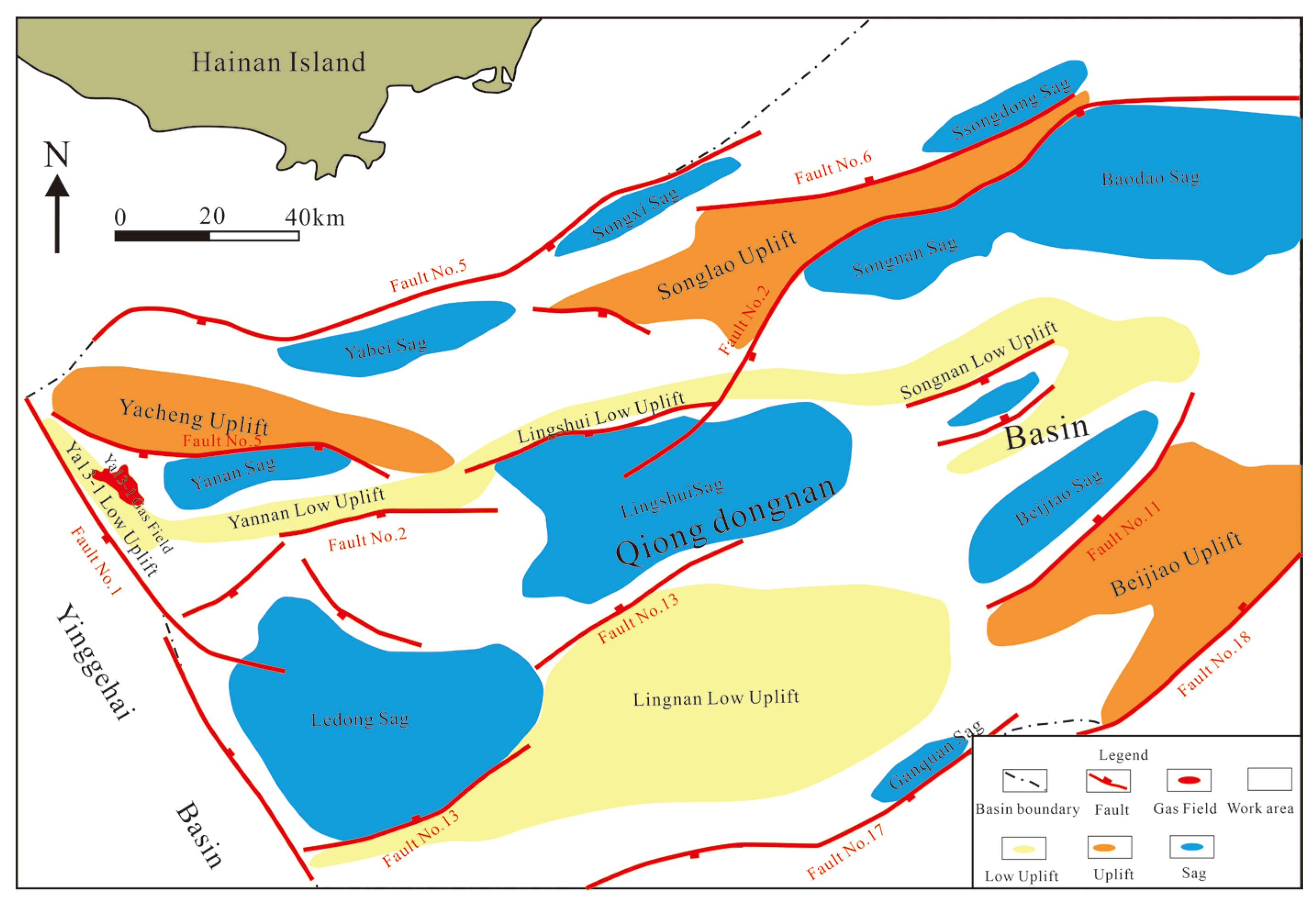
The Qiongdongnan Basin (QDNB) is a Cenozoic basin located on the continental shelf in the northern part of the South China Sea (Figure 1). The basin is separated from the Yinggehai Basin by the Deep Great Rift in the west, from the Zhujiangkou Basin by the Shenhu Uplift in the east, the Hainan Uplift in the north and the Xisha Uplift in the south. The QDNB comprises five secondary tectonic units: the Hainan Uplift, the Northern Depression, the Central Uplift, the Central Depression and the Southern Uplift. The QDNB has undergone two phases of tectonic evolution, the Paleoproterozoic Faulting Stage and the Neoproterozoic Depressional Stage, forming a typical ‘double-layered structure’ of the faulted basin. The basin is filled from bottom to top by the Eocene, YC and Lingshui formations in the Paleocene rifting stage, and the Sanya, Meishan, Huangliu and Yinggehai formations in the Neoproterozoic depression stage. The QDNB is an important target for deep-water exploration in the South China Sea, and AVO technology has been used to achieve good results in this area [11,12]. Fluid-sensitive information extracted from pre-stack information can effectively reduce the multi-solution of strong amplitude highlights, and several medium and large oil and gas fields in LS17-2, LS18-1 and LS25-1 have been discovered, demonstrating good exploration prospects [13,14]. However, with the progressive exploration, the large reservoir targets were exhausted and then shifted to the turbidite waterway sandstone with more complex stratigraphic assemblage, which is limited by the high cost of deep-water exploration, few drilling wells and the uncertainty of AVO in the thin layer, putting forward higher requirements on AVO analysis for deep-water exploration. In this study, the LS31 channel in the QDNB in the western part of the South China Sea is taken as the target area.
3. Methods
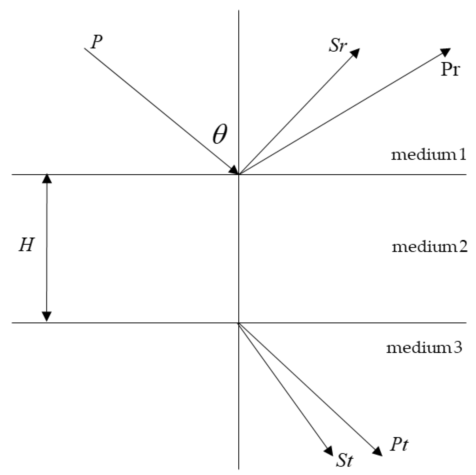
The theory of thin layer reflection coefficient, which discusses the reflection and transmission propagation of a plane wave in the layered medium from the perspective of elastic wave dynamics, is based on the Brekhovski equation. Suppose two semi-infinite elastic media are sandwiched by the horizontal media (Figure 2). If the thickness of the stratum is less than one wavelength, the fluctuations at the interface between the top and bottom of this stratum will interfere and superimpose significantly, so that the fluctuations formed at the top surface of the thin layer will have different characteristics from those of the thick layer in all aspects of intensity variation and waveform characteristics. The result of the superimposed reflection depends mainly on the thickness of the thin layer, the propagation velocity of the thin layer and the angle of incidence of the plane wave.
3.1. Theory of Thin Layer Reflectance Coefficient
Let the plane wave be incident from the top layer into the below layer, and the angle of incidence of the P-wave into each layer is , then the displacement function expressions for each wave in the top layer [15] can be expressed as
where , is respectively the displacement functions of the incident and the reflected P-wave; , is respectively the displacement functions of the incident and reflected S-wave; , is respectively the amplitudes of P-wave and S-wave; , is respectively upward and downward wave; is angular frequency; is time; , , is respectively the number of horizontal waves in the longitudinal direction, the number of vertical waves in the longitudinal direction and the number of vertical waves in the transverse direction.
The displacement-stress relationship can be expressed as
where superscripts 1, 2 and 3 is respectively the first, second and third layer of the medium; , is respectively the displacement function; is the vertical stress; is the horizontal stress; is the propagation matrix; superscript 2 is the propagation matrix related to medium 2.
The formulae for calculating the reflection and transmission coefficients [16] can be expressed as
where , , , is respectively longitudinal reflection coefficient, transverse reflection coefficient, longitudinal transmission coefficient and transverse transmission coefficient; , is P-wave and S-wave velocity.
Reflected waves from the thin interlayer in multilayered media are composite waves formed by the superposition of a single wave in the thin interlayer after different numbers of reflections, so recursive algorithm can be used to calculate the displacement and stress relationship between the top and bottom of the thin interlayer, so that the reflection transmission coefficient of each layer can be found.
where ,, can be expressed as
where , , , . is slowness in the horizontal direction; , is respectively P-wave and SV-wave slowness; , is respectively P-wave and SV-wave vertical slowness; H is the thickness of the stratum.
3.2. Thin Layer AVO Curves Versus Stratigraphic Thickness
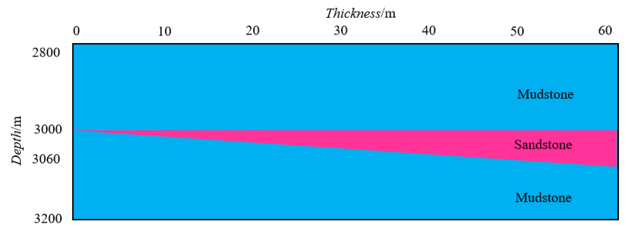
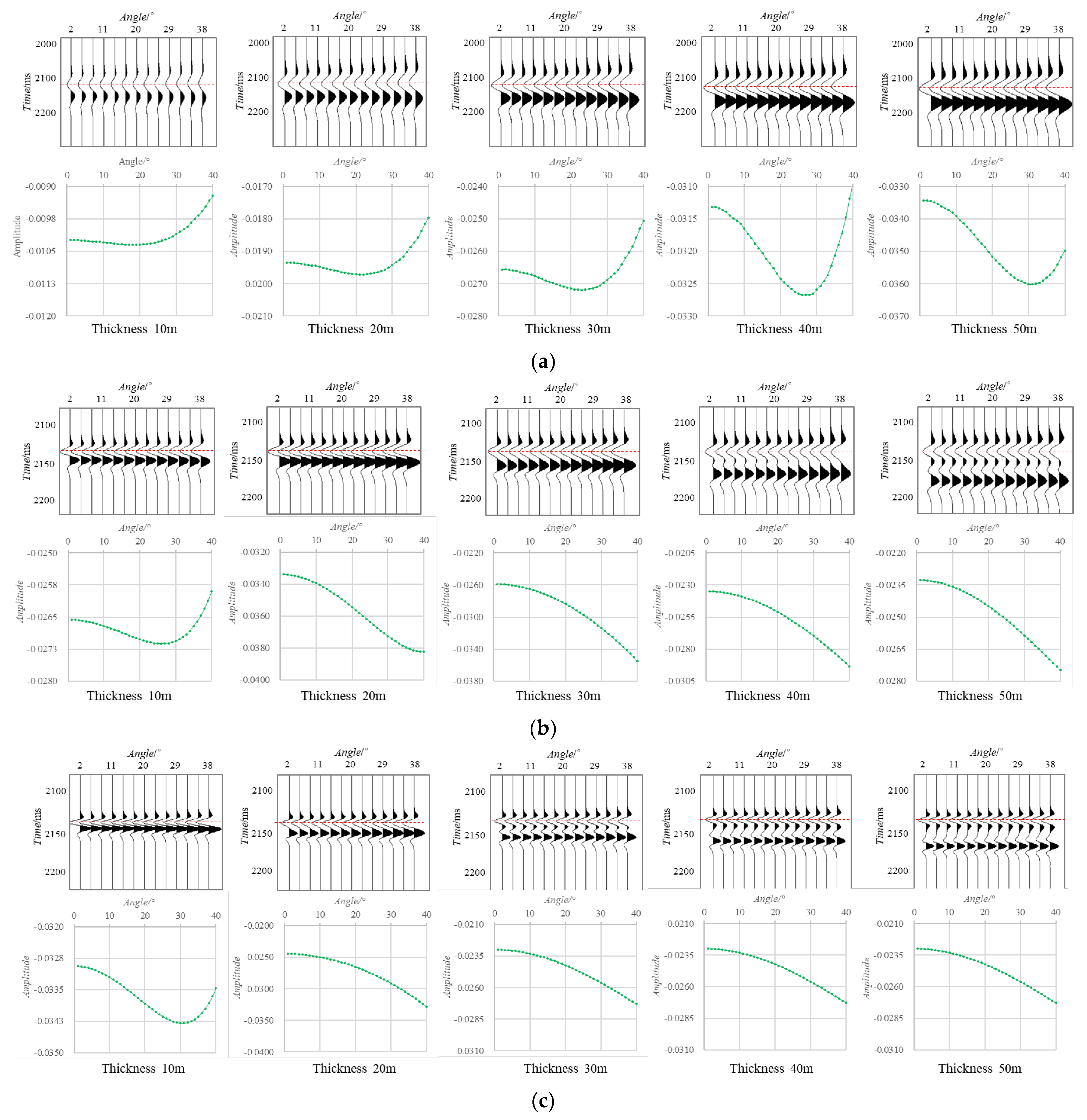
When the thickness of the thin layer is equal to one quarter of the seismic wavelength, the seismic wave field appears to interfere in the same phase, making the amplitude appear extremely large, and this phenomenon is called the tuning effect of the thin layer. In order to analyze the relationship between the thickness of the thin layer, the main seismic frequency and its pre-stack AVO characteristics, a single sand wedge model is designed (Figure 3), and the elastic parameters of the wedge model are shown in Table 1. The results of the pre-stack AVO simulation are shown in Figure 4. When the stratigraphic thickness is greater than the tuning thickness, the simulated results show that the top surface of the sandstone exhibits III AVO characteristics, which is basically the same as the actual AVO characteristics of the stratigraphic layer, and the variation of amplitude with the angle is more-or-less stable without much different, indicating that the simulation results of the thin layer reflection coefficient formula and the Zoeppritz equation are the same when the stratigraphic thickness is thicker than the tuning thickness.
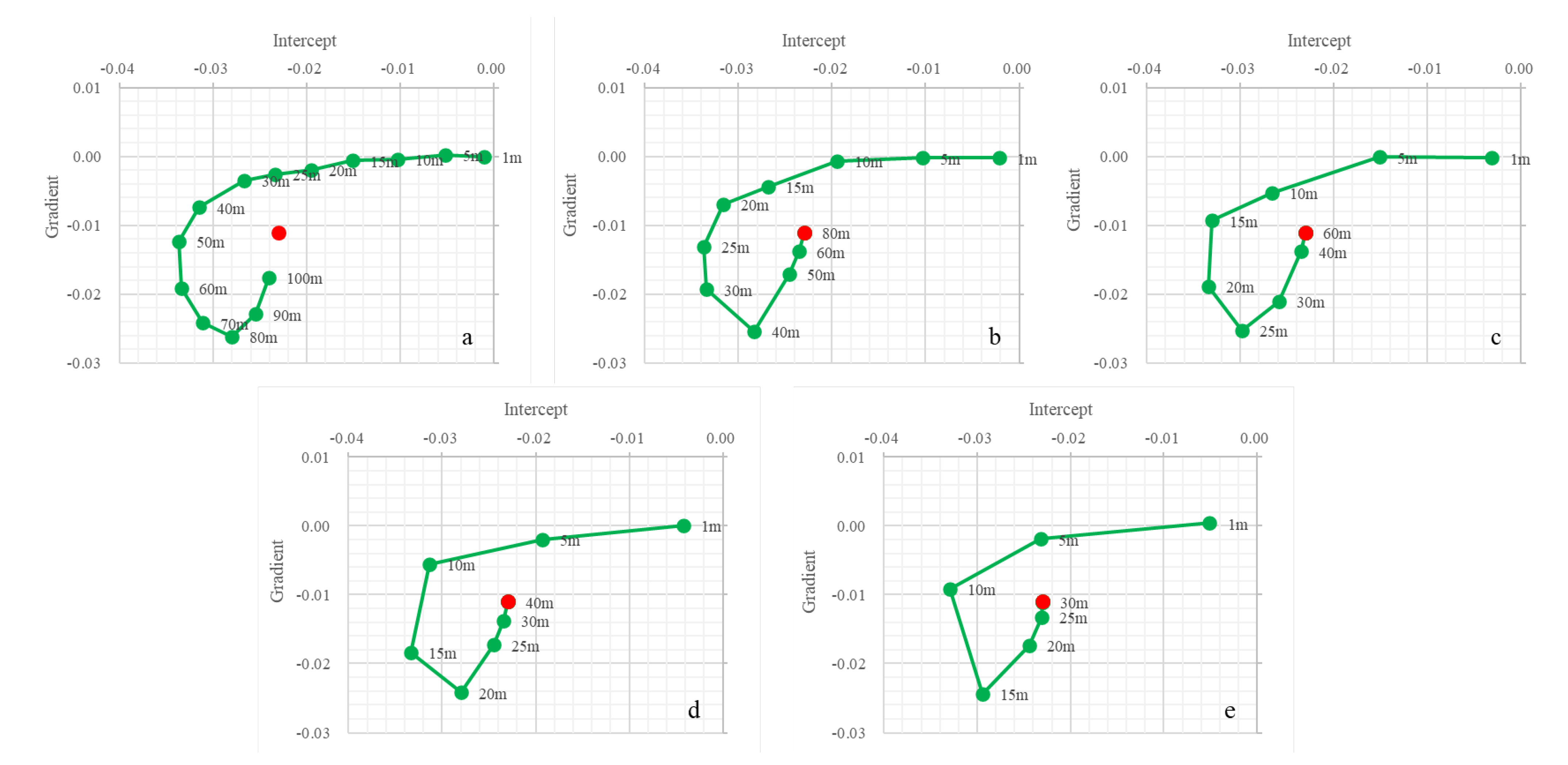
We performed rendezvous analysis of the intercept and gradient of the simulation results for different dominant frequencies (Figure 5). As a whole, there is a spiral distribution in the intercept and gradient rendezvous, with different dominant frequencies having different abilities to identify the thin layer. For the dominant frequency of 10 Hz (where half-wavelength = 137.5 m), when the thickness of the layer is less than a half-wavelength, the intercept and gradient of the top surface of sandstone is less than a half-wavelength deviation from their true values (red dots are the values of the Zoeppritz equation calculation when the thickness of the layer is half-wavelength) due to the interference between the top and bottom reflection interfaces. When the dominant frequency is 20 Hz (half-wavelength = 68.75 m), the intercept gradient converges to the same position for sandstone thicknesses greater than a half-wavelength, and basically does not change with the thickness of the formation. However, when the sandstone thickness is less than a half-wavelength, the intercept and gradient are principally influenced by the thickness of the formation: when the sandstone thickness is less than the tuning thickness, the intercept increases with the sandstone thickness; when the sandstone thickness is greater than the tuning thickness, the intercept decreases with the sandstone thickness and the gradient follows a similar pattern of change characteristics, but the position of the inflection point is delayed. As the dominant frequency gradually increases, the wavelength progressively decreases (45.8 m at 30 Hz half-wavelength, 34.4 m at 40 Hz half-wavelength, and 27.5 m at 50 Hz half-wavelength, using the layer P-wave velocity of 2750 m/s), and the intercept and gradient converge to the true value of the layer when the layer thickness exceeds a half-wavelength, and the higher the main frequency the better the recognition of the thin layer.
3.3. AVO Detuning Effect Analysis Based on Sparse Inversion
In the tuning thickness range, how to correct the amplitude and phase data, remove the tuning effect and the stretching effect, and restore the influence of the offset factors on the waveform, is the key to the successful application of AVO technology [17,18,19]. The previous studies show that the top-bottom interference in the tuning thickness range has a large impact on the thin layer’s true AVO relationship, and here a sparse inversion strategy is introduced to the detune effect method.
Theoretically, zero-offset seismic traces have only wavelet and stratigraphic tuning effects, while non-zero offset traces have offset tuning effects in addition to wavelet and stratigraphic tuning effects. The fitted AVO detuning inversion uses the AVO attribute as the model’s spatial parameter, and uses the Shuey approximation formula to obtain the attribute parameter model without the tuning effect by fitting the approximation to the actual pre-stack seismic trace set data with the tuning effect.
The binomial approximation of AVO reflection coefficient [20] can be expressed as
where is the reflection coefficient, is the intercept, is the gradient, is the angle. The above equation can also be expressed in matrix form
where , .
The detuning effect inversion problem can be expressed [21] as
where is actual pre-stack seismic data. is the intercept and gradient matrix after detuning effects.
Whether it is the acoustic impedance tuning effect or the elastic tuning effect, the parameters are not independent, and the seismic data itself is noisy (especially the far offset seismic data, which is noisier) which further increases the degree of ambiguity of the parameter variables. The inversion problem is severely unsuitable due to multiple parameters, non-independence between parameters, and noise. In order to adapt the inversion problem to reduce the multi-solution nature of the inversion, constrained inversion is generally performed [22,23]. In this paper, we propose the use of the constraint sparse inversion method of model parameters and seismic data. The inverse problem can be expressed as
where is sparse optimization results for reflection coefficients or reflection amplitudes.
The seismic pre-stack gather is the convolution of the reflection coefficient and wavelet, and the seismic record is projected onto the wavelet to achieve sparse transformation. The degree of sparsification is related to the band width of the wavelet: the wider the band width of the wavelet, the narrower the wavelet pulses in the time domain, and the greater the degree of sparsification of the seismic record after the sparse transformation by wavelet projection [24,25]. The main parts of this sparsification process include the creation of a wavelet dictionary library and hierarchical sparsification.
Firstly, for wavelet dictionary library building, wavelet vector can be expressed as
Secondly, hierarchical sparsification. A basic idea of sparse reconstruction is to arrange and intercept data from the largest to the smallest, and the sparsity is the number of selected data from the largest to the smallest. If a signal is continuous and has a certain distribution, the complete signal can be reconstructed with fewer samples. The reflection coefficients are not continuously predictable in the longitudinal direction, and the corresponding seismic records are also not continuously predictable in the longitudinal direction [26,27,28]. To address these problems, we propose a hierarchical sparsification reconstruction method. The method is based on the following idea: for a section of a seismic record, the maximum and minimum values (absolute values) are obtained, and the data are divided into multiple sequences of different levels from large to small at a certain segmentation spacing, and then each sequence is reconstructed by sparse reconstruction, and finally the reconstruction results of each level are then weighted and summed.
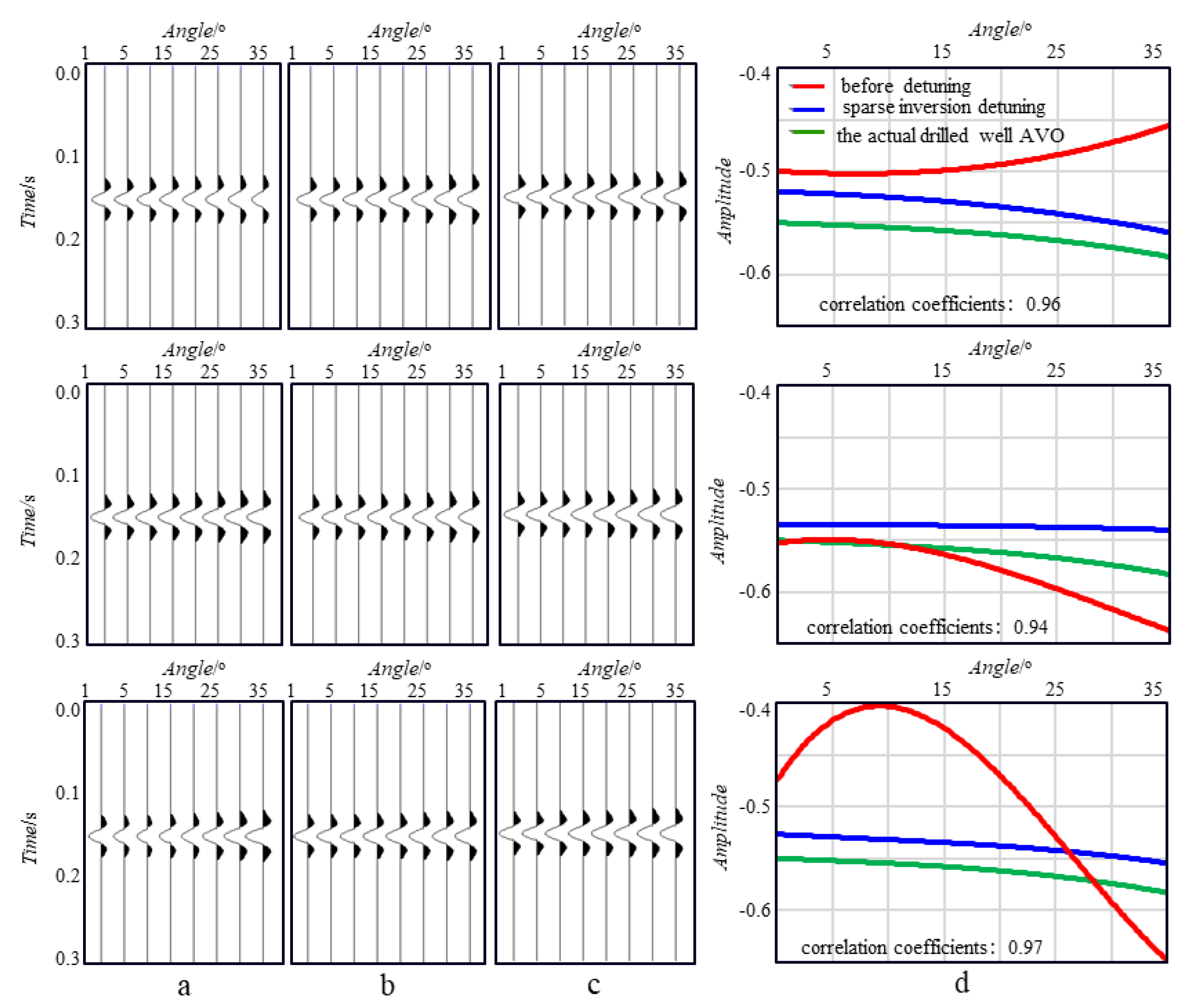
In order to verify the reliability of this technical method, this paper randomly designed a geological model with different thin layer combinations for pre-stack forward simulation (Figure 6), where the stratigraphic real shows III AVO response characteristics, and only the stratigraphic combination of the thin layer is changed. The analysis of the forward simulation shows that the actual stratigraphy has both III and IV AVO characteristics due to the tuned influence of the thin stratigraphic assemblage, indicating that the tuning effect has changed the real AVO of the actual stratigraphy, resulting in some uncertainty in the AVO analysis. The sparse inversion strategy proposed in this paper is used to detune this effect, and the correlation analysis with the theoretical orthodromic shows that (i) the de-coupling effect and the theoretical orthodromic AVO types basically match each other, showing III AVO response characteristics, and (ii) the correlation coefficients with the theoretical orthodromic AVO can reach above 90%, which can better reflect the real AVO response characteristic of thin gas-bearing sandstones and effectively reduce the multi-solvability of AVO analysis.
4. Results
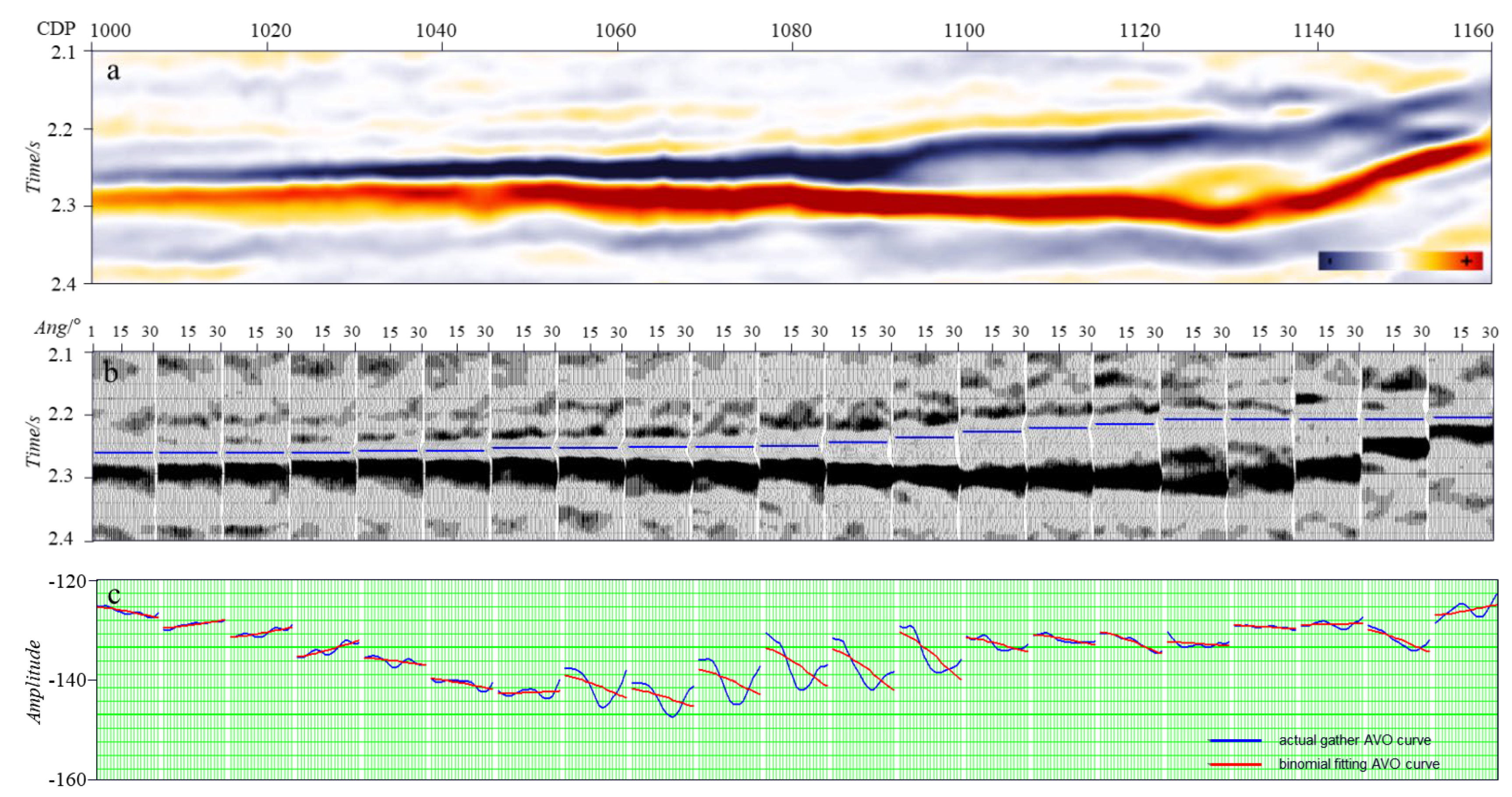
LS31 channel, which is located in the QDNB of the South China Sea, is geological conditioned for developing large and medium-sized oil and gas fields [29,30,31]. A statistical analysis of the AVO types of sandstone reservoirs in this area at different depths shows that the reservoir in the central canyon channel in the deep-water area has good physical properties: the gas-bearing sandstones are mostly IV AVO, the gas-bearing sandstones away from the canyon channel are mostly III AVO, most of the water-bearing sandstones show IV AVO characteristics [32,33], and the gas-water difference is relatively obvious. Consider the post-stack seismic profile and the pre-stack gather across the LS31 channel as an example (Figure 7). In the post-stack seismic profile, the channel features are obvious, with the top surface of the channel showing negative-phase trough reflections and the bottom surface showing positive-phase reflections and obvious undercutting features, with the middle thickening and the sides gradually thinning. However, in the pre-stack gather, the AVO characteristics of the top surface of the LS31 channel vary greatly due to the influence of the change in the thickness from the edge to the main body of the channel, and III AVO and IV AVO existing between each other, especially at the position of the tuned thickness; therefore, the AVO curve shows an obvious V-shape variation, with III AVO characteristics at small angles in the near gathers and IV AVO at large angles in the far gathers. This makes the analysis of AVO in this area very difficult.
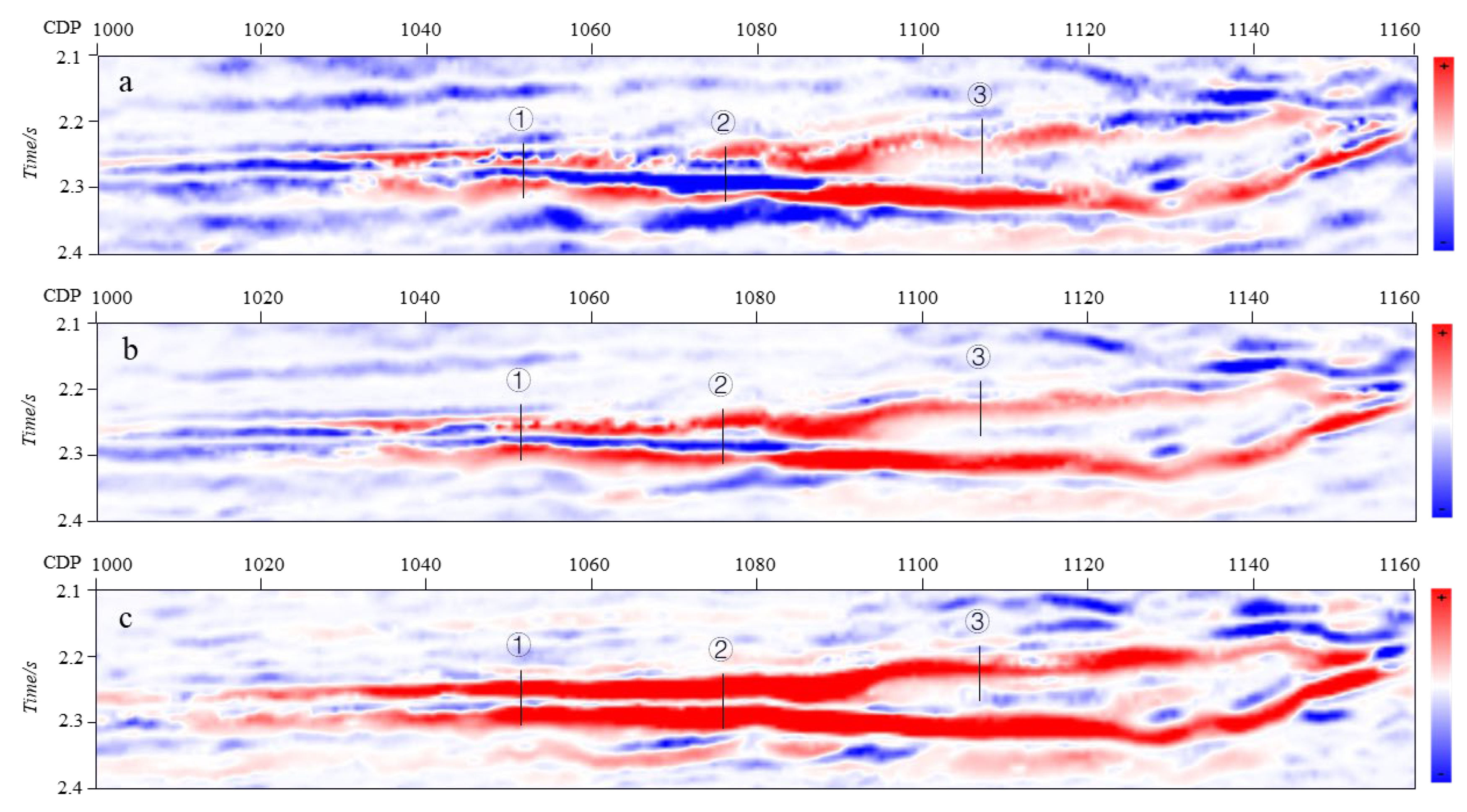
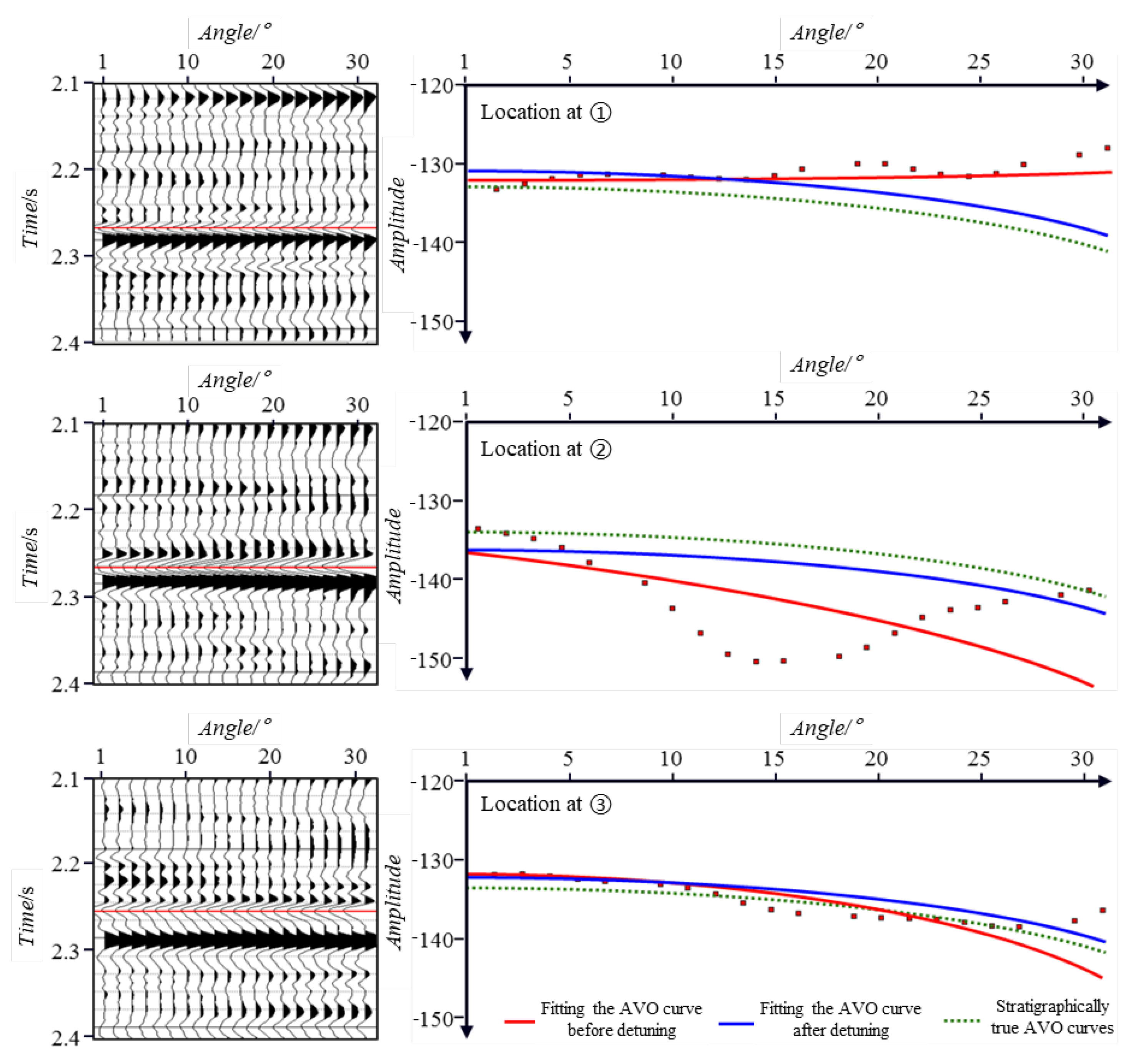
We use the detuning method proposed in this paper to compare and analyze the PG attribute profiles of the high and low parts of the LS31 channel, and the AVO change characteristics before and after the detuning (Figure 8). Before the correction of the PG attribute (Figure 8a), due to the interference of sandstone thickness, the high and low parts of the target area are mostly dominated by III AVO and IV AVO coexistence, and the AVO anomaly of the sandstone in the main body of the LS31 channel is not clear. We also show the detuned profile using the conventional method (waveform correction) due to the influence of stretching factors, and also the near and far channel frequency change due to the gun inspection distance, and thus the tuning effect of AVO is not effectively improved (Figure 8b). After the correction of the detuning effect via sparse inversion (Figure 8c), the AVO anomalies in the high and low parts of the target area are relatively consistent, all showing mainly III AVO, and the AVO variation characteristics before and after detuning are basically consistent with the actual stratigraphic AVO, and the V-shape feature on the single point AVO gather is practically eliminated (Figure 9).
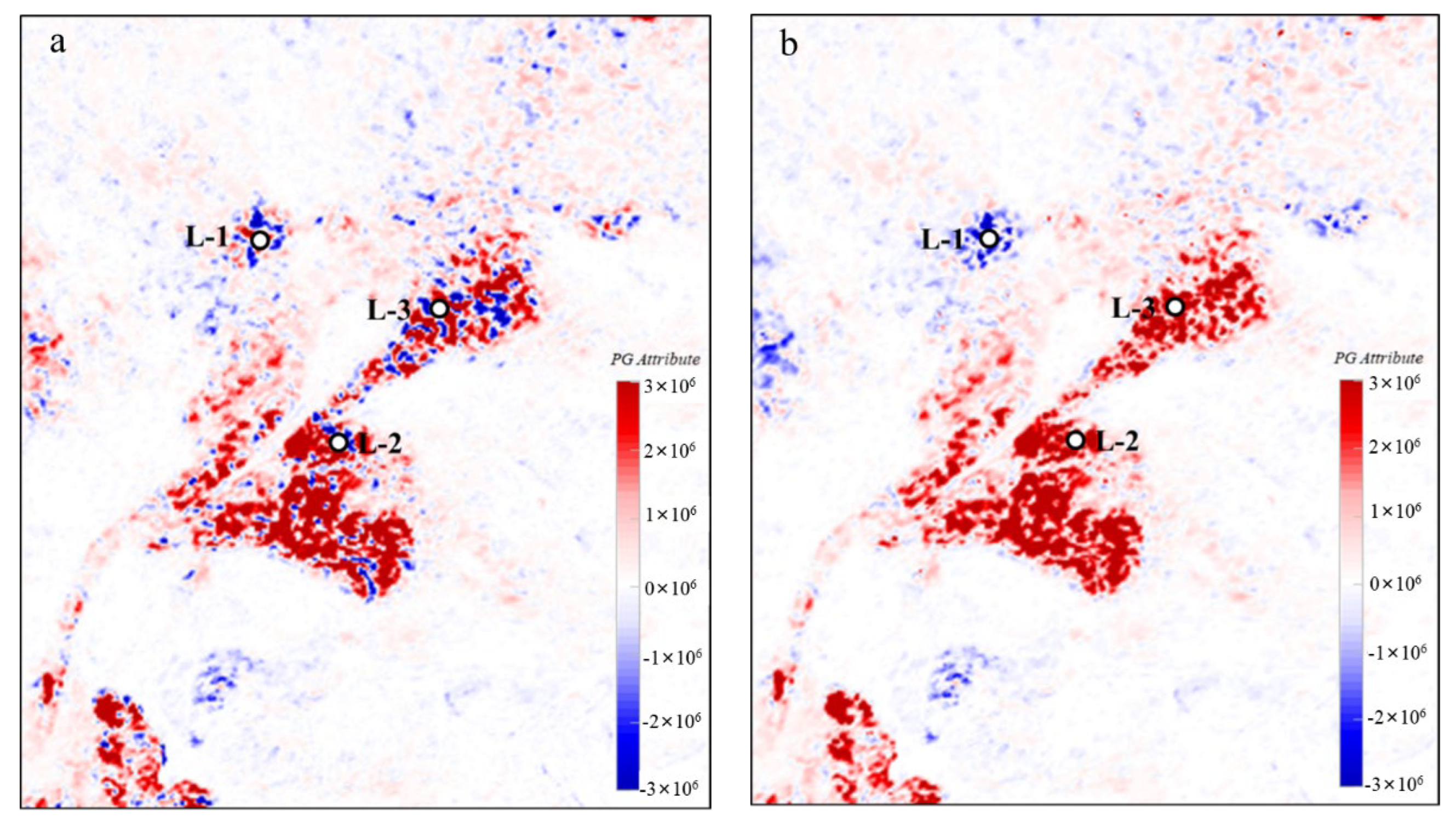
From the AVO attribute extracted before and after detuning (Figure 10), it can be seen that the pre-detuning AVO shows the coexistence of III and IV AVO, and after correction by sparse inversion detuning, the influence of the detuned V-shape on AVO is basically eliminated, which is basically consistent with the actual drilled wells. The L-1 well encountered 18 m of water-bearing sandstone in the Yinggehai Formation, which exhibited IV AVO characteristics, which correlates with what was observed after detuning; however, before detuning the AVO characteristics were not obvious, and both III and IV AVO characteristics were observed. Combining the detuned PG attributes, drilling well L-2 was deployed in the main part of the Yinggehai Formation, producing a high-quality gas reservoir of 41.8 m with a porosity of 20.8%, adding approximately 9.6 billion cubic meters of proven reserves. Subsequently well L-3 is to be drilled to progress and expand the scale of reserves. This technology has opened up a new dimension of exploration in the shallow Yinggehai Formation in the Lingshui Depression, and has effectively promoted the exploration and development process of the deep-water gas fields in the western part of the South China Sea.
5. Conclusions
The forward simulation analysis of tuned AVO in thin reservoirs reveals that the difference in the tuning effect of near gathers and far gathers in the tuning thickness range is a key factor leading to the multiresolution of thin AVO. In order to solve this problem, the AVO detuning effect method based on the sparse fitting inversion strategy is studied, which can better solve the problem of multi-solutions of multivariate coupled inversion. At the same time, the fitted AVO inversion method can effectively remove the AVO tuning effect and reduce the uncertainty of AVO analysis in thin reservoirs, which is more beneficial to the AVO inscription analysis of thin reservoirs. The DF gas field and LD gas field in Yinggehai Basin are also faced with the uncertainty of AVO analysis of thin reservoirs. The technical method proposed in this paper has been effectively verified and applied in the small well area of Yinggehai Basin, and could be further employed to solve the uncertainties experienced at other wells, both in this Basin and beyond.
Author Contributions
Conceptualization, W.S.; Data curation, X.W.; Investigation, X.Z.; Methodology, S.L.; Software, A.Y., X.W. and Y.L. All authors have read and agreed to the published version of the manuscript.
Funding
This research received no external funding.
Conflicts of Interest
The authors declare that they have no known competing financial interests or personal relationships that could have appeared to influence the work reported in this paper.
References
- Widess, M.B. How thin is a thin bed? Geophysics 1973, 38, 1176–1180. [Google Scholar] [CrossRef]
- Kallweitt, R.S.; Wood, L.C. The limits of resoulution of zero-phase wavelets. Geophysics 1982, 47, 1035–1046. [Google Scholar] [CrossRef]
- Zeng, H.L.; John, A.; Katherine, G. How thin is a thin bed: An alternative perspective. In Proceedings of the 2008 SEG Annual Meeting, Las Vegas, NV, USA, 9–14 November 2008; pp. 834–838. [Google Scholar]
- Simmons, J.L.; Backus, M.M. Amplitude-versus-offset modeling and the locally converted shear wave. In Proceedings of the 1993 SEG Annual Meeting, Washington, DC, USA, 26–30 September 1993; pp. 738–741. [Google Scholar]
- Liu, Y.B.; Schmitt, D.R. Quantitative analysis of thin layer effects: Transmission coefficients and seismograms. In Proceedings of the 2000 SEG Annual Meeting, Calgary, AB, USA, 6–11 August 2000; pp. 2464–2467. [Google Scholar]
- Pan, W.Y.; Innanen, K.A. AVO/AVF analysis of thin-bed in elastic media. In Proceedings of the SEG Houston 2013 Annual Meeting, Houston, TX, USA, 22–27 September 2013; pp. 373–377. [Google Scholar]
- Wang, X.; Yu, S.; Li, S.; Zhang, N. Two parameter optimization methods of multi-point geostatistics. J. Pet. Sci. Eng. 2022, 208, 109724. [Google Scholar] [CrossRef]
- Lu, S.Q. Application of prestack frequency-division AVO analysis method in Luojia area. Geophys. Prospect. Pet. 2013, 52, 151–156. [Google Scholar]
- Guo, Z.Q.; Liu, C.; Feng, X. Reflection characteristics of thin reservoirs and its AVO attributes analysis. Geophys. Prospect. Pet. 2009, 48, 453–458. [Google Scholar]
- Wang, X.; Zhang, F.; Li, S.; Dou, L.; Liu, Y.; Ren, X.; Chen, D.; Zhao, W. The Architectural surfaces characteristics of sandy braided river reservoirs, case study in Gudong oil field, China. Geofluids 2021, 2021, 8821711. [Google Scholar] [CrossRef]
- Huang, H.T.; Huang, B.J.; Huang, Y.W. Condensate origin and hydrocarbon accumulation mechanism of the deepwater giant gas field in western South China Sea: A case study of Lingshui 17-2 gas field in Qiongdongnan Basin, South China Sea. Pet. Explor. Dev. 2017, 44, 380–388. [Google Scholar] [CrossRef]
- Zhao, B.; Li, Z.; Gao, C.; Tang, Y. Identification of complex fluid properties in condensate gas reservoirs based on gas-oil ratio parameters calculated by optimization mathematical model. Front. Energy Res. 2022, 10, 863776. [Google Scholar] [CrossRef]
- Zhang, G.C.; Zeng, Q.B.; Su, L. Accumulation mechanism of LS 17-2 deep water giant gas field in Qiongdongnan Basin. Acta Petrol. Sin. 2016, 37, 34–46. [Google Scholar]
- Yao, Z.; Wang, Z.F.; Zuo, Q.M. Critical factors for the formation of large-scale deepwater gas field in Central Canyon System of Southeast Hainan Basin and its exploration potential. Acta Petrol. Sin. 2015, 36, 1358–1366. [Google Scholar]
- Wu, F.Y.; Ma, P.Y.; Huang, M.L. Thin reservoirAVO analysis of spectral reflection coefficient. Prog. Geophys. 2010, 25, 71–75. [Google Scholar]
- Chang, S.L.; Zhang, S.; Liu, J.; Liu, Z.L.; Chen, Q.; Liu, B. Influence of surrounding rock changes on the coal seam reflected wave under thin interbed condition. Coal Geol Explor. 2021, 49, 220–229. [Google Scholar]
- Chen, S.; Lu, R.; Liu, L.H. Analysis of the influence of thin interbed interference on prestack AVO attributes. Earth Sci. Front. 2020, 27, 98–109. [Google Scholar]
- Liu, L.B.; Wang, Y.G.; Sun, C.Y. Thin inter-bed AVO characteristics analysis based on forward model. Oil Geophys. Prospect. 2019, 54, 1246–1253. [Google Scholar]
- Wang, X.; Zhou, X.; Li, S.; Zhang, N.; Ji, L.; Lu, H. Mechanism study of hydrocarbon differential distribution controlled by the activity of growing faults in faulted basins: Case study of paleogene in the Wang Guantun area, Bohai Bay Basin, China. Lithosphere 2022, 2021, 7115985. [Google Scholar] [CrossRef]
- Shuey, R.T. A simplification of the Zoeppritz equations. Geophysics 1985, 50, 609–614. [Google Scholar] [CrossRef]
- Di, H.B.; Guo, Y.Q.; Liu, X.W. Relative acoustic impedance inversion based on Cauchy sparseness constraint Bayesian estimation. Geophys. Prospect. Pet. 2011, 50, 124–128. [Google Scholar]
- Meng, X.J.; Du, S.T. Log-constrained polynomial fitting extrapolation inversion of seismic data. Oil Geophys. Prospect. 1995, 30, 363–372. [Google Scholar]
- Zhang, Y.F.; Ling, F.; Cheng, B.J. Application of well log constrained seismic trace inversion combined with polynomial fitting. Oil Gas Geol. 2001, 22, 388–390. [Google Scholar]
- Chen, Z.Q.; Wang, J.B. A spectral inversion method of sparse-spike reflection coefficients based on compressed sensing. Geophys. Prospect. Pet. 2015, 54, 59–466. [Google Scholar]
- An, H.W.; Li, Z.W.; Li, R.F. Application of sparse impulse impedance inversion in YX oil field. Geophys. Prospect. Pet. 2002, 41, 56–60. [Google Scholar]
- Kang, Z.L.; Zhang, X.B. Seismic sparse deconvolution based on L1/2 regularization. Geophys. Prospect. Pet. 2019, 58, 855–863. [Google Scholar]
- Wang, X.; Liu, Y.; Hou, J.; Li, S.; Kang, Q.; Sun, S.; Ji, L.; Sun, J.; Ma, R. The relationship between synsedimentary fault activity and reservoir quality—A case study of the Ek1 formation in the Wang Guantun area, China. Interpretation 2020, 8, sm15–sm24. [Google Scholar] [CrossRef]
- Song, W.Q.; Zhang, Y.; Wu, C.R.; Hu, J.L. The method of weak seismic reflection signal processing and extracting based on multitrace joint compressed sensing. Chin. J.Geophys. 2017, 60, 3238–3245. [Google Scholar]
- Yao, G.S.; Yuan, S.Q.; Wu, S.G.; Zhong, C. Double provenance depositional model and exploration prospect in deepwater area of Qiongdongnan Basin. Pet. Explor. Dev. 2008, 35, 685–691. [Google Scholar] [CrossRef]
- Huang, B.J.; Li, L.; Huang, H.T. Origin and accumulation mechanism of shallow gas in the North Baodao slope, Qiongdongnan Basin, South China Sea. Pet. Explor. Dev. 2012, 39, 530–536. [Google Scholar] [CrossRef]
- Wang, X.; Hou, J.; Li, S.; Dou, L.; Song, S.; Kang, Q.; Wang, D. Insight into the nanoscale pore structure of organic-rich shales in the Bakken Formation, USA. J. Pet. Sci. Eng. 2020, 191, 107182. [Google Scholar] [CrossRef]
- Zhang, Y.M.; Niu, C.; Han, L.; Ye, Y.F. A method of frequency dispersion AVO analysis and its application in deep water area of South China Sea. China Offshore Oil Gas 2016, 28, 21–27. [Google Scholar]
- Liu, S.Y.; Zhang, Y.Z.; Li, Y.S. Application of far and near trace attributes for AVO analysis in deep water area in Qiongdongnan basin. Coal Geol. Explor. 2020, 48, 197–202. [Google Scholar]
Figure 1.
Primary geological structures and the regional stratigraphy in the study area.

Figure 2.
Schematic diagram of thin layer reflection and transmission.

Figure 3.
Theoretical Wedge mode.

Figure 4.
Characteristics of AVO response before stacking, and the amplitude variation curve at different angles for wedge model. (a) The dominant frequencies of wavelet is 10 Hz (the tuning thickness is 68.75 m). (b) The dominant frequencies of wavelet is 30 Hz (the tuning thickness is 22.90 m). (c) The dominant frequencies of wavelet is 50 Hz (the tuning thickness is 13.75 m).

Figure 5.
Intercept and gradient rendezvous plots for different dominant frequencies. (a) 10 Hz; (b) 20 Hz; (c) 30 Hz; (d) 40 Hz; (e) 50 Hz.
Figure 5.
Intercept and gradient rendezvous plots for different dominant frequencies. (a) 10 Hz; (b) 20 Hz; (c) 30 Hz; (d) 40 Hz; (e) 50 Hz.

Figure 6.
Theoretical model validation of the effects of detuning AVO. (a) before detuning AVO; (b) sparse inversion detuning AVO; (c) the actual drilled well AVO; (d) AVO change curve with angle.
Figure 6.
Theoretical model validation of the effects of detuning AVO. (a) before detuning AVO; (b) sparse inversion detuning AVO; (c) the actual drilled well AVO; (d) AVO change curve with angle.

Figure 7.
Seismic result profile and corresponding pre-stack gather for LS31 channel. (a) post-stack seismic section; (b) pre-stack gathers; (c) AVO variation curve of pre-stack gathers.
Figure 7.
Seismic result profile and corresponding pre-stack gather for LS31 channel. (a) post-stack seismic section; (b) pre-stack gathers; (c) AVO variation curve of pre-stack gathers.

Figure 8.
Comparative analysis of PG attribute profiles before and after detuning correction of the LS31 channel. (a) PG profiles before detuning; (b) PG profiles after detuning by conventional method; (c) method in this paper.
Figure 8.
Comparative analysis of PG attribute profiles before and after detuning correction of the LS31 channel. (a) PG profiles before detuning; (b) PG profiles after detuning by conventional method; (c) method in this paper.

Figure 9.
Comparative analysis of AVO characteristics before and after detuning (location①②③ at Figure 8).
Figure 9.
Comparative analysis of AVO characteristics before and after detuning (location①②③ at Figure 8).

Figure 10.
AVO attributes before and after detuning in the Yinggehai Formation, LS31 channel. (a) PG attributes before detuning; (b) PG attributes after detuning.
Figure 10.
AVO attributes before and after detuning in the Yinggehai Formation, LS31 channel. (a) PG attributes before detuning; (b) PG attributes after detuning.


Table 1.
The elastic parameters of the wedge model.
| AVO | Mudstone Enclosures | Sandstone | Zoeppritz Calculation | |||||
|---|---|---|---|---|---|---|---|---|
| P-Wave (m·s−1) | S-Wave (m·s−1) | Density (g cm−3) | P-Wave (m·s−1) | S-Wave (m·s−1) | Density (g cm−3) | Intercept | Gradient | |
| III | 2810 | 1480 | 2.53 | 2750 | 1750 | 2.12 | −0.023 | −0.011 |
Publisher’s Note: MDPI stays neutral with regard to jurisdictional claims in published maps and institutional affiliations. |
© 2022 by the authors. Licensee MDPI, Basel, Switzerland. This article is an open access article distributed under the terms and conditions of the Creative Commons Attribution (CC BY) license (https://creativecommons.org/licenses/by/4.0/).
Share and Cite
MDPI and ACS Style
Liu, S.; Song, W.; Zhou, X.; Yan, A.; Wang, X.; Li, Y. AVO Detuning Effect Analysis Based on Sparse Inversion. Energies 2022, 15, 5202. https://0-doi-org.brum.beds.ac.uk/10.3390/en15145202
AMA Style
Liu S, Song W, Zhou X, Yan A, Wang X, Li Y. AVO Detuning Effect Analysis Based on Sparse Inversion. Energies. 2022; 15(14):5202. https://0-doi-org.brum.beds.ac.uk/10.3390/en15145202
Chicago/Turabian StyleLiu, Shiyou, Weiqi Song, Xinrui Zhou, Anju Yan, Xixin Wang, and Yangsen Li. 2022. "AVO Detuning Effect Analysis Based on Sparse Inversion" Energies 15, no. 14: 5202. https://0-doi-org.brum.beds.ac.uk/10.3390/en15145202
Note that from the first issue of 2016, this journal uses article numbers instead of page numbers. See further details here.