


CFD Modeling of Pressure Drop through an OCP Server for Data Center Applications


1
Design and Simulation Technologies, Inc., 26480 Eskisehir, Turkey
2
Department of Civil Engineering, Eskisehir Osmangazi University, 26480 Eskisehir, Turkey
3
Lande Industrial Metal Products Inc. Co., Organized Industrial Zone, 20th Street, No: 14, 26110 Eskisehir, Turkey
*
Author to whom correspondence should be addressed.
Energies 2022, 15(17), 6438; https://0-doi-org.brum.beds.ac.uk/10.3390/en15176438
Submission received: 30 July 2022
/
Revised: 28 August 2022
/
Accepted: 29 August 2022
/
Published: 3 September 2022
(This article belongs to the Special Issue Advanced Computational Fluid Dynamics Modeling)
Abstract
:Modeling IT equipment is of critical importance for the simulations of flow and thermal structures in air cooled data centers. Turbulent flow undergoes a significant pressure drop through the server due to the energy losses originating from the internal components. Therefore, there is an urgent need to develop a fast and an accurate method for the calculation of pressure losses inside server components for data center applications. In this study, high resolution numerical simulations were performed on an OCP (Open Compute Project) server under various inlet flow rates for inactive and active conditions. Meanwhile, one key challenge of modeling complete geometry of the server results from using an intense mesh even for a single server. To address this challenge, the server was modeled as a porous zone to mimic inertia and viscous resistance in a realistic way. Comparison of the results of porous and complete models showed that the proposed model could calculate pressure drop accurately even when the number of cells in the server was reduced to 0.3% of the complete model. Porosity coefficients were determined from the numerical simulations conducted in a broad range of air discharge for both active and inactive conditions. Errors in the calculation of pressure drop may result in a significant deviation in the prediction of the temperature rise over the server. Thus, the present model can effectively be used for the fast and accurate prediction of pressure drop inside a server component rather than solving internal flow on an intense mesh, while simulating airflow inside an air-cooled data center, which is crucial for the design safety of data centers. Finally, calculated porosity coefficients can be used for the prediction of the pressure drop in a server, while designing data centers based on numerical simulations.
1. Introduction
Data centers are becoming more and more widespread nowadays with the dizzying developments in Information Technologies (IT), such as Internet of Things (IoT), cloud computing, big data, and mobile applications. Power consumption of a data center is essentially composed of the IT equipment and cooling devices. Flow and thermal distributions in an air-cooled data center substantially influence the cooling efficiency and power consumption of the cooling devices. A well-designed thermal environment is suggested in a data center for the mitigation of hot air recirculation and cold air bypass, as well as for the reduction of power consumption by the cooling. Recently, rapid developments in the Computational Fluid Dynamics (CFD) technologies have emerged as powerful tools for the design of data centers based on the simulation of flow and thermal structures [1]. Modeling IT equipment is of critical importance in the realistic simulation of thermal distribution including physical effects, such as heat generation, fan driven air flow, and energy losses.
Thermal mass approach can be effectively used for the thermal modeling of servers and racks in the CFD modeling of data centers. Khankari [2] proposed a simplified model to include thermal mass of the rack and air assuming that the heat transfer between the rack and room occurs along the exposed side and top of the rack. Ibrahim et al. [3] used the server thermal mass by adding density and specific heat to the racks to represent server components in the data center modeling. The proposed thermal mass approach substantially influenced the temperature distribution inside the data center. Ibrahim et al. [4] developed thermal mass of a 2U server based on the experimental measurements. Zhang and VanGilder [5] added various cooling failure modes, unit fans, circulation pumps, and chillers to the model developed by Abi-Zadeh and Samain [6], where the entire data center is idealized as a single rack and cooling unit. Sundaralingam et al. [7] presented a well-mixed model to direct inlet and exhaust air to a specific location, including the thermal masses of the rack, rack contents and other objects in the flow area. Ibrahim et al. [8] developed a compact CFD model and explained the importance of the thermal mass and heat exchange between the server and airflow. Lin et al. [9] investigated transient performance of a data center considering aisle enclosure and chilled water storage tank. Van Gilder et al. [10] proposed a compact server model that can be directly incorporated into the data center model. Hot components were found to be increasing at a very slow rate inside the server. Alkharabsheh et al. [11] developed a detailed model to consider calibrated fan curves and leak locations for servers and cooling units. Pressure drop forming between inlet and outlet of a server accounts for the energy dissipation resulting from the interaction of the turbulent flow with the internal components, such as graphical card, CPU, heat exchanger, and fans. Volumetric resistance models developed based on the experimental measurements were also used for the prediction of the pressure drop in the rack level modeling [12,13]. However, detailed simulations of the turbulent flow through a complete server model have been less well investigated. On the other hand, complete modeling of a server including internal micro-components makes it impossible for the simulation of overall thermal distribution of a data center in terms of computational memory and time [14]. A fast and accurate numerical model is required for the optimal design of a data center since CFD models have evolved to the simulation-optimization frameworks with the developments in open-source technologies and artificial intelligence (AI) in recent years [15,16,17].
It is important to accurately characterize the pressure drop between components in a rack and to avoid unnecessary obstacles within the server. CFD simulation was performed by combining pressure drop test results for servers at different heights and fan curves for IT equipment [12]. Components inside a server create a significant pressure drop. This pressure drop is a function of the airflow rate that cools the server and affects the amount of energy needed by the fans. This flow-blocking resistance can be modeled as a porous medium. The porosity value in the server can be calculated by equalizing the pressure drop in the Hagen–Poiseuille flow based on the hydraulic diameter of a typical 1U server [18]. The liquid inlet temperature and flow rate are the most effective parameters that can affect the efficiency of the cold plate technology. The reduced pressure drop across the cold plate and the thermal resistance between the surface temperature and the coolant temperature have a major impact on the thermal performance and energy savings of data centers. A significant decrease in the thermal resistance and average surface temperature were observed with increasing water flow [19]. However, a substantial increase is observed in the pressure drop and pumping power as well. The serpentine cold plate has better thermal performance but higher pressure drops and pumping power compared to the parallel cold plate designs [20]. The porous model can consider the pressure drop in a flow region and simulate the conditions encountered as the fluid passes through the porous media. This approach can be used also in the thermal analysis of heat exchangers and electronic devices [21]. The porous media approach can reduce the mean temperature error from 2 K to 0.77 K compared to the black-box approach [22]. Zhou et al. [23] utilized Darcy–Forchheimer equations for the modeling of IT equipment and validated model results with the experimental data. Gupta et al. [24] found that the relationship between pressure drop and flow rate was linear. As a result of the numerical studies, it is concluded that the porous environment can be used as an effective approach for the simulation of airflow in the design of data centers [25].
The focus of the current effort is to develop a fast and an accurate method for the prediction of the pressure drop along IT equipment, while simulating thermal and flow distributions in data centers. To achieve this goal, a series of numerical simulations were performed using various inlet velocities over the Leopard V3.1 model of the OCP server shown in Figure 1. Spatial variation of the averaged pressure along the server was analyzed in detail. A porous model was developed based on the simulation data for the calculation of pressure drop without solving internal flow on an intense mesh. Results of the complete and porous models were analyzed to show reliability of the proposed model.
2. Methods
2.1. Governing Equations
Airflow through the server can be modeled by the following continuity and momentum equations for the incompressible and turbulent flow:
where () denotes mean velocity components in three directions x1, x2, x3, is the Reynolds stress term, p is the mean pressure, are the Cartesian coordinates, t is the time, is the kinematic viscosity of the fluid, is the gravitational acceleration in the i-direction, and is the momentum source, which is defined in the porous region. An eddy viscosity model is used for the calculation of the Reynolds stresses in Equation (2):
where k is the turbulent kinetic energy, is the turbulent viscosity, and is the Kronecker delta. In order to account for the separation of turbulent flow from the internal micro-components, the SST turbulence closure model is preferred using the following transport equations for turbulent kinetic energy k and the specific dissipation rate in a two-equation turbulence model [26]:
Finally, turbulent viscosity can be calculated from the following equation:
where and
are empirical coefficients of the turbulence closure mode and can be found in [25]. The maximum Mach number of the air flow is calculated as 0.01. Density of the air can be assumed to be constant since the variation of the density is less than 5% when the Mach number is less than 0.3 [27]. Moreover, internal components of the server are modeled as solid objects with no heat dissipation in the fluid domain. Therefore, an incompressible solver is used in the simulation of the turbulent flow [28].
2.2. Computational Domain, Boundary Conditions and Mesh
A virtual wind tunnel (VWT) was created for the simulation of the airflow through the server. As shown in Figure 2, inlet and outlet of the VWT were located at distances of 0.5 L and L from the server, respectively. Here, L is the length of the server. Face zones were created just upstream and downstream of the server to calculate average pressures for the calculation of pressure drop taking into account spanwise variations.
Boundary conditions were defined for the velocity u, pressure p and turbulence variables (k and ) at the boundaries of the computational domain in Figure 2. A fixed average velocity was imposed at the inlet and zero gradient boundary condition was applied for the velocity at the outlet. Pressure was fixed to atmospheric pressure at the outlet and a zero gradient boundary condition was used at the inlet. Application of the Drichlet-type boundary conditions for the velocity and pressure enhances the stability of the numerical model. Turbulence quantities were calculated according to 5% turbulence intensity at the inlet [29] and zero gradient boundary condition was used at the outlet. No-slip boundary condition was used for the velocity, zero gradient boundary condition was used for the pressure, and wall functions were used for the turbulence variables at the walls. In order to a maintain a freestream flow at the upstream and downstream of the server, slip boundary conditions were used at front, back, bottom, and top faces of the domain. Mathematical definitions of the boundary conditions are given in Table 1. Here, unified wall functions for and calculate variables at the center of the cell adjacent to the wall depending on the dimensionless wall distance. The “calculated” boundary of OpenFoam in Table 1 calculates turbulence viscosity from the and as at the inlet.
A hexahedra (hex) and split-hex mesh was created using snappyHexMesh utility from the STL (Stereolithography) model of the server with parallel computing even if the parallel computing took approximately two hours for the accurate snapping of triangulate surfaces. The resulting mesh, shown in Figure 3, consists of 5.98 million cells, which is extremely high for a transient simulation since the Courant number suggests smaller time step sizes due to stability issues. Statistics of the mesh are summarized in Table 2. Skewness and non-orthogonality of the mesh were found to be appropriate for the calculation of gradients over the cell faces. Steady-state simulations were performed using various inlet conditions on an intense mesh. However, a transient simulation was also carried out for a single inlet condition to compare results with the steady-state results in the latter part of the study. Results of the previous solution were imported as an initial condition to the current solution during successive simulations to achieve steady-state solution using less iteration. In addition, a residual control algorithm was developed using the decreasing trend of the residual approach for the termination of steady-state iterations in a smart manner and incorporated into the open-source model (see Software availability).
2.3. Numerical Method
Numerical simulations were performed using open-source CFD code OpenFoam [30], which employs a finite volume method for the discretization of governing equations over a control volume. Convective terms were discretized using second-order accurate linear-upwind divergence scheme and gradient terms were discretized using second-order accurate Gauss linear method. First-order accurate Euler method was used for the discretization of time derivatives during transient simulation. Thus, the steady-state model is second-order accurate in space, the transient model is first-order accurate in time and second-order accurate in space. The Semi-Implicit Method for Pressure-Linked Equations (SIMPLE) was used in the steady state solutions and the PIMPLE method, which is the combination of the Pressure Implicit with the Splitting of Operator (PISO) and the SIMPLE methods, was used in the transient simulation. Equations were discretized implicitly using the fvm option of OpenFoam and coefficients were stored into three matrices of owner, neighbor, and diagonal for each equation in the segregated solution of the governing equations. The resulting matrices can be solved using built-in iterative linear solvers available in OpenFoam [30]. Numerical simulations were performed with parallel computing using 56 processors on TRUBA (Turkish National Science e-Infrastructure) resources. OpenFoam cases of active and inactive servers were publicly distributed [31].
In order to determine whether the solution reaches steady-state or not, an object function was developed and incorporated into the open-source CFD model considering three conditions. The first condition compares the residual between two successive iterations with a selected relative tolerance of 1 × 10⁻⁶, which can be calculated by using standard functions in OpenFoam. The second condition checks whether the iteration number is less than the maximum iteration number, which was selected as 20,000 in the controlDict file. The last condition, which is developed in the present study, calculates the residual for each variable using the least squares method considering the last 20% of the residuals in the log-scaled space. This condition is achieved when the convergence slope is less than 0.05 as a horizontal trend line. As shown in Figure 4, residuals tend to decrease in the logarithmic scale and the solution reaches steady-state when the iteration number is 1721. Here, horizontal and vertical axis were normalized with respect to the maximum iteration number and maximum value of the residual in the log-space to interpret gradients in a specific range. The last condition is invoked by the object function after the iteration number of 1500 to speed up solutions. The source code of the object function is available at the GitHub repository given in the software availability part of this study.
3. Results
3.1. Validation of the Numerical Method
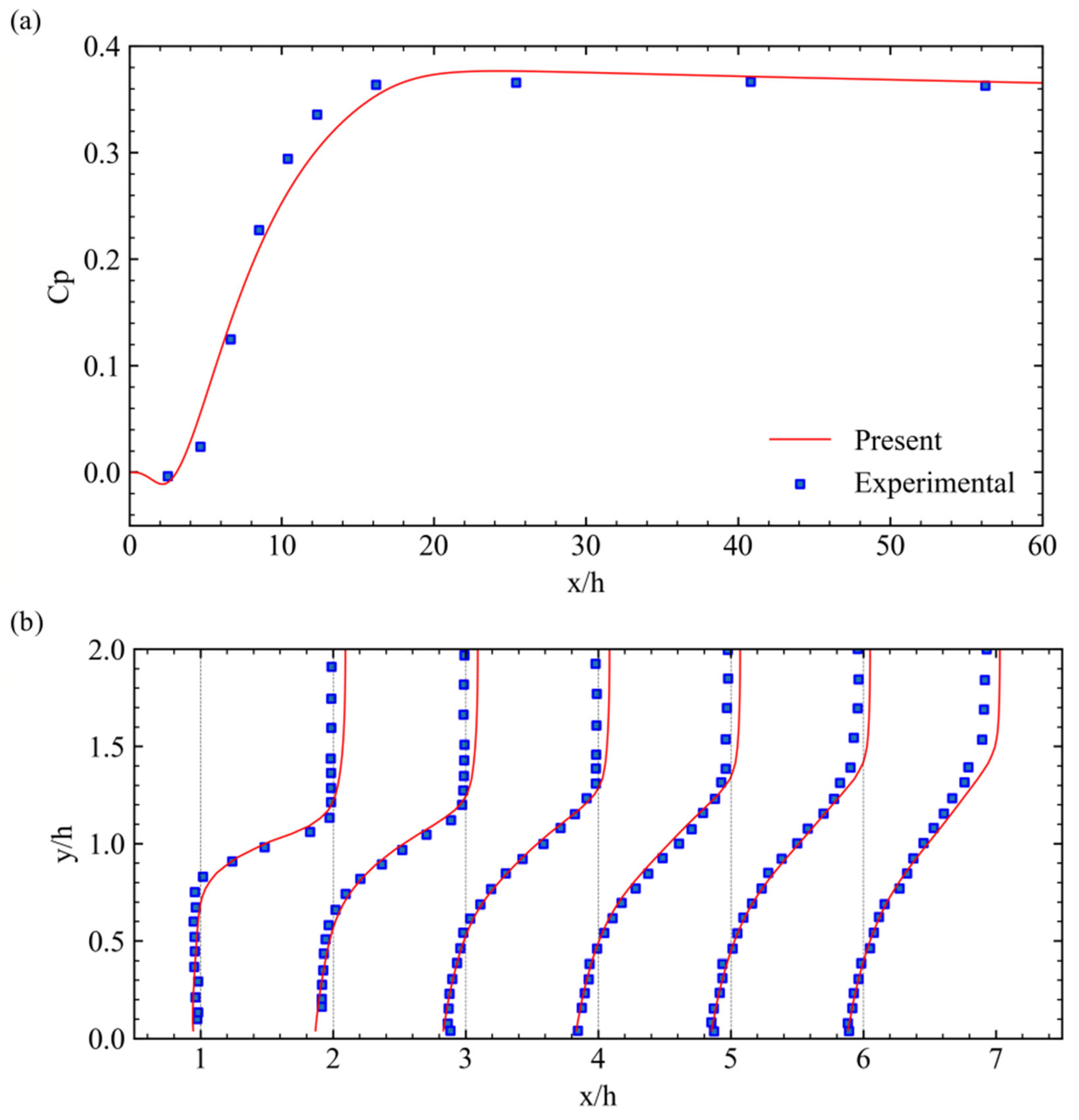
In order to validate the computational model, turbulent flow through an axisymmetric sudden expansion is simulated and numerical results are compared with the experimental measurements by means of laser Doppler anemometer (LDA) for the velocity and pressure tapping for the pressure in a wind tunnel [32]. Geometrical features of the problem are given in Figure 5. Inlet and outlet dimeters of the channel are selected as mm and mm and step height is selected as mm. The expansion ratio of the channel is 2 for this channel configuration. A uniform velocity is applied at the inlet of the channel to adjust the same Reynolds number of , as in the experimental studies.
Variations of the pressure coefficients for the numerical and experimental results in Figure 6a show that the present numerical model can predict the pressure variation in a channel in the presence of a local change in the flow domain. Figure 6b shows comparison of the calculated axial velocities with the LDA measurements. The present numerical model and wall functions are capable of calculating flow velocities accurately. Thus, the present numerical framework can be used for the simulation of the incompressible flow through a server consisting local changes.
3.2. Investigation of the Internal Flow Field
A mesh independence study was carried out for the flowrate of 0.03 m3/s using five mesh resolutions to find the optimum mesh resolution that yields accurate solution. As seen in Figure 7, the pressure drop was estimated higher for lower mesh sizes due to the lacks of cell numbers and cell sizes near the internal components. Lack of the mesh resolution resulted in a minimum pressure drop when the number of cells is approximately 4 million. Numerical simulations show that the results become independent of the mesh resolution when the mesh size is approximately 5.98 million. This mesh was used in the rest of the simulations conducted in the present study.
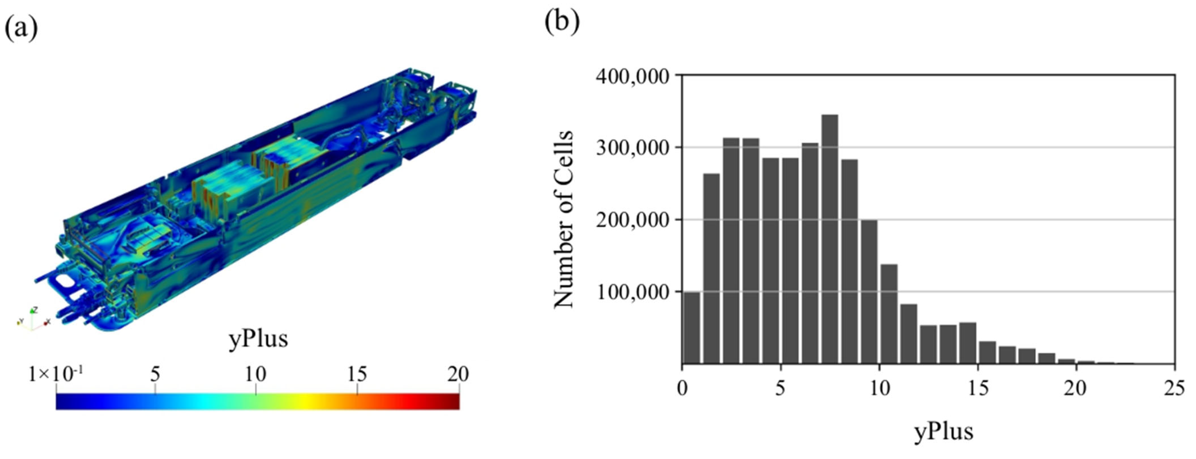
Figure 8 shows distribution of the dimensionless wall distance over the server walls and histogram of the y+ values throughout the computational domain to check whether the present mesh can capture wall effects, such as separation and reattachment. Figure 8b shows that a great amount of the cells coincides within the viscous sub layer. Thus, the present mesh is fine enough to resolve boundary layer that develops over the walls.
Results obtained from steady-state and transient simulations are compared in Figure 9 in terms of the distributions of velocity and pressure along the server. Note that spanwise averaged velocity and pressure values were used in Figure 9. Time-averaging was conducted during transient simulation and time-averaged values were compared with the steady-state results. Consistency between steady-state and transient results confirms that the unsteady fluctuations in the transient simulations are not effective on the time-averaged results. Thus, steady-state results can be reliably used for the estimation of the pressure drop along the server.
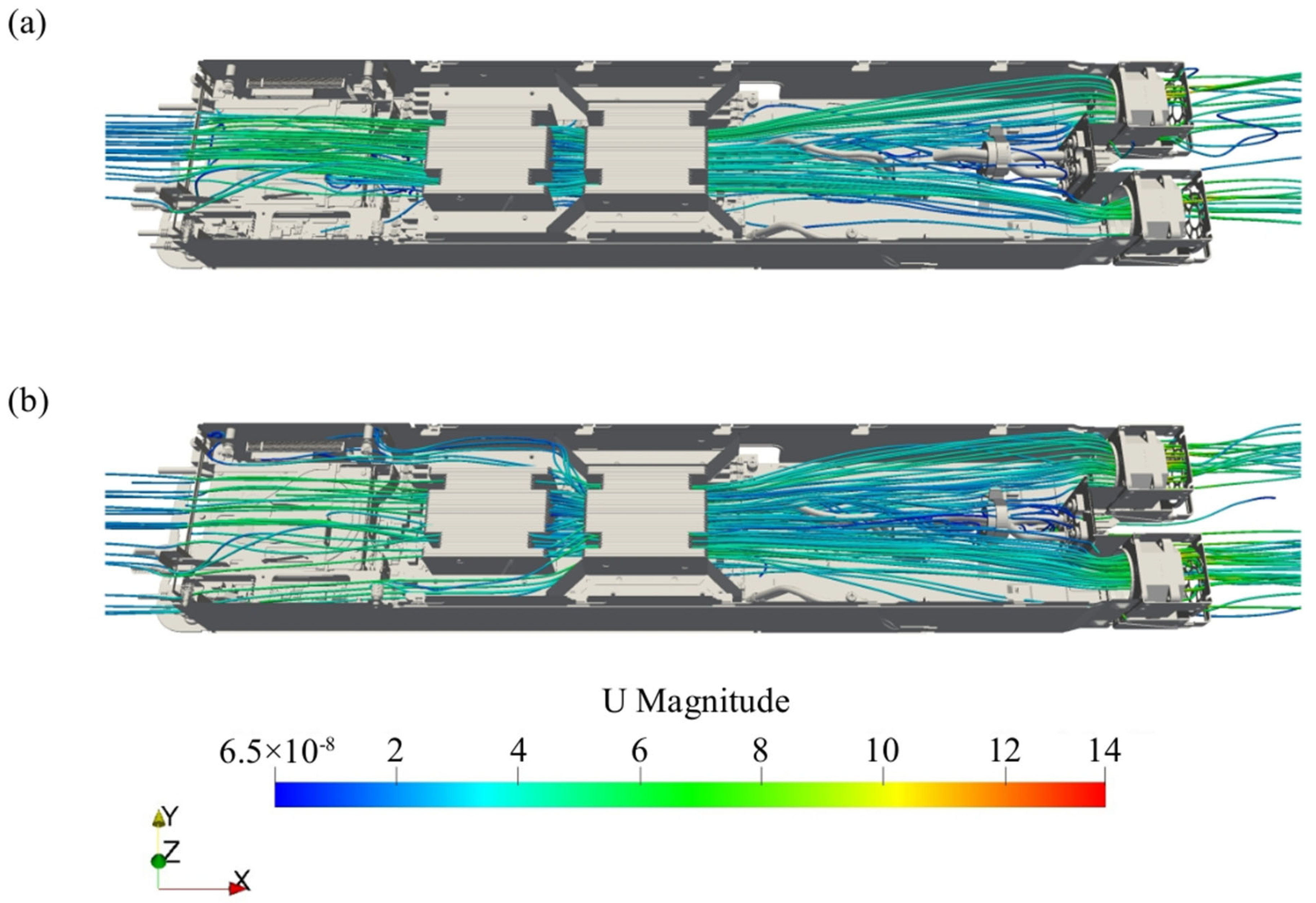
Investigation of the internal flow field through the server is of importance to examine the underlying mechanism in pressure drop and to understand at which locations the energy dissipation increases, which may lead to new server designs for high cooling efficiency. The main concern regarding the internal flow field is whether the heat sinks benefit from adequate cold air to maintain the maximum CPU temperature below the suggested value by the manufacturer. Three-dimensional streamlines in Figure 10 reveal that the rear heat sink benefits the cold air more than the front sink with the effects of air guides located at the entrance of the heat sink. Heat transfer between fluid and solid regions needs to be modeled using the Conjugate Heat Transfer (CHT) model for better understanding of the mechanism between heat generation and cooling.
Variation of the static pressure over the midplane of the server in Figure 11 shows a significant pressure drop from the inlet to the outlet of the server. Low pressures are created by fans to maintain a turbulent flow from the inlet to the outlet with an adequate flow rate to benefit from the cold air supplied by the Computer Room Air-conditioning (CRAC) units. Flow rate passing through the server is substantially influenced by the specifications of the fans. Thus, an appropriate server model is required to calculate the flow rate of a server for both black-box and open-box modeling of server components in the simulation of thermal distribution in a data center.
3.3. Development of a Porous Model for the Server
The present numerical study provides a detailed description of the internal flow field forming inside the server. However, complete modeling of servers in a data center requires a huge memory and long computational duration to calculate pressure drops accurately. It is possible to conduct experimental studies in a wind tunnel to measure pressure drop between entrance and exit of a server for various inlet velocities. However, an expensive experimental infrastructure including wind tunnel and measurement devices is required for this experimental study, which is not a sustainable way for server manufactures. On the other hand, uncertainties arising from the experimental studies may also reduce reliability of the experimental data. To mitigate this challenge, we propose a porous model for the calculation of pressure drops in a rapid way since the porous approach described here can mimic resistance effects caused by the internal components of the server. As shown in Figure 12, a porous region was created inside VWT with the same dimensions as in the complete model (Figure 2). A block-structured orthogonal mesh was created using blockMesh utility and the resultant mesh consists of 20,352 cells, which is approximately 0.3% of the complete model. Such a big economy in cell numbers will significantly reduce computational memory and time, which is important in data center applications.
A porous zone was generated using topoSet utility in OpenFoam and the following source term is added to the momentum equations at the cells inside the porous zone to mimic inertia and viscous resistance using Darcy–Forchheimer porosity model [1,14,25,33].
where D and F are the Darcy and Forchheimer coefficients, respectively. The critical step in the porous modeling of a server is the prediction of these empirical coefficients for the corresponding server model. In this study, a set of numerical simulations were performed for the flow rates between 0.003 and 0.06 m3/s with 20 simulations. Servers in a data center can be classified as active and inactive depending on the workloads. A server can be called an active server when a workload is assigned to the server and an inactive server when the server is in an idle condition. Thus, the present numerical model should calculate pressure drop occurring in a server for both active and inactive servers. Fans are considered as stationary solid boundaries during numerical simulations, which is valid for inactive servers. As seen in Figure 13, fans were removed from the CAD model of the server and numerical simulations were repeated without fans. This approach is applicable to full working servers when the fan curves are used for the prediction of the flow rate since fan curves are obtained considering the effects of the server blades. Thus, fans were not considered in the numerical simulations of active server.
In order to obtain porosity coefficients in Equation (7) depending on the inlet conditions, a series of numerical simulations were performed using various inlet velocities. Pressure drops were calculated and variation of the pressure drop with the inlet velocity is plotted in Figure 14. Here, D and F coefficients were determined using the least squares method from the results of the complete model. Sheth and Saha [25] suggested the porosity of a server between 0.35 and 0.65. Darcy and Forchheimer coefficients were determined for a porosity of 0.5, a hydraulic diameter of 0.55, and results are compared with the present results in Figure 14. The large discrepancy observed between previous and current approaches proves that the selection of the porosity coefficients significantly influences the accuracy and reliability of the results. Moreover, estimation of the porosity for a server model is challenging in practice. Thus, the present approach can be effectively used in practice without need of estimating porosity of the server. The pressure drop can be formulated using the following equation:
where L is the length of the porous zone and is the viscosity of the fluid. The pressure drop can be approximated to the results obtained from the fully resolved three-dimensional simulations by choosing appropriate D and F coefficients. In this study, the following least squares method is used to determine coefficients in Equation (8).
The minimum value of the error in the above equation yields the best fit values of D and F coefficients. Calculated D and F coefficients are given for inactive and active servers in Table 3. As seen in Figure 14, the approach proposed by Sheth and Saha [25] increases prediction error for porous modeling of inactive servers. These coefficients can be used, while modeling the present OCP server using the proposed porous approach in the future studies without solving internal flow field, which will speed up simulation of flow and thermal structures in data centers.
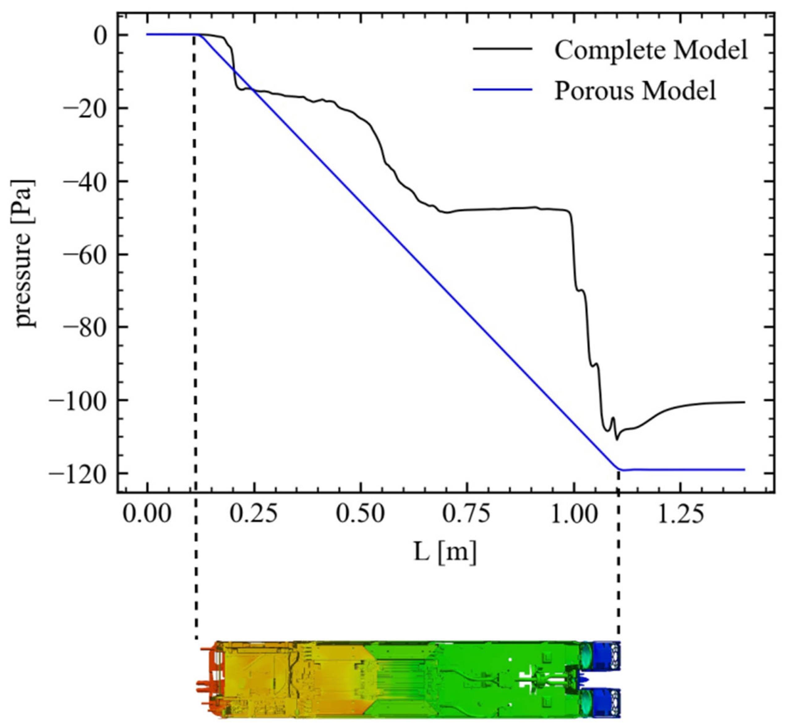
Variation of the spanwise averaged pressure along the server in Figure 15 depicts sudden drops near the inlet, rear heat sink, and outlet. The pressure drop observed at the inlet section may increase when the PCI (Peripheral Component Interconnect) cards or perforated covers are used at the inlet. The second pressure drop occurs at the rear heat sink since most of the flow is directed here. The pressure drop at the front heatsink, however, is relatively low due to the openings at both sides. The last and the highest pressure drop observed at the outlet section is associated with the existence of fans as local changes in the flow environment.
The uncertainty observed in Figure 15 can be estimated from the following uncertainty index (UI):
where and are predicted pressure drops in complete and porous models, respectively. The UI is calculated for the tested flow rates and given in Table 4 for active and inactive servers. Uncertainty of the results are observed higher in inactive servers than active servers for small flow rates since fans induce high pressure drop when the flow rate reduces.
4. Conclusions
The current study is relevant to the prediction of pressure drop through server components in the thermal modeling of air-cooled data centers. High-resolution numerical simulations were performed over an OCP server using an open-source CFD model. An object function was developed and incorporated into the open-source model to detect whether the solution reaches steady-state or not. Comparison of the transient and steady-state results showed that the steady-state results are identical to the time-averaged results. The steady-state results indicated that significant pressure drop observed near the inlet, rear heatsink, and fans should be taken into consideration in the CFD analysis of data centers. A series of numerical simulations were carried out for active and inactive servers by using various inlet conditions to obtain variation of the pressure drop with the inlet velocity. In order to calculate the pressure drop in a rapid way, the server was modeled as a porous region considering inertia and viscous resistance caused by the internal components. Porosity coefficients were determined using the least squares method from the generated numerical data for the active and inactive servers. Comparison of the results of porous and complete models showed that the proposed porous model could be reliably used for the fast and accurate prediction of the pressure drop along the server component even when the mesh size was reduced to 0.3%. Porosity coefficients determined for active and inactive conditions can be used as an input parameter, while modeling OCP servers in the thermal simulations of air-cooled data centers. The virtual wind tunnel (VVT) approach proposed in the present study is considered to be more sustainable for server manufacturers than conducting experimental measurements in a wind tunnel.
The internal flow structure of a server plays an important role in maintaining the maximum CPU temperature below a threshold value recommended by the manufacturer. Numerical simulations showed that the rear heat sink benefited from the cold air more than the front one with the effects of air guides located at the entrance of the heat sink. Furthermore, the present numerical study reveals the internal flow structure of the server, which may lead to the optimal design of the layout of the internal components over a server not only to maximize the cooling efficiency but also to minimize the energy reduction. Finally, the numerical framework developed in this study can be integrated to a conjugate heat transfer (CHT) model for the thermal safe design of the server as a future study.
Author Contributions
Data curation, M.K. and C.Y.; Formal analysis, E.D.; Funding acquisition, C.Y.; Investigation, A.D. and M.K.; Methodology, A.D. and E.D.; Project administration, E.D.; Software, A.D., S.Y. and M.K.; Supervision, E.D.; Validation, A.D.; Visualization, A.D. and S.Y.; Writing—original draft, S.Y., M.K. and E.D.; Writing—review & editing, E.D. All authors have read and agreed to the published version of the manuscript.
Funding
This paper is part of a project that has received funding from the European Union’s Horizon 2020 research and innovation program under grant agreement No 956059. The opinions stated in this deliverable reflects the opinion of the authors and not the opinion of the European Commission.
Data Availability Statement
Source code; https://github.com/DSTECHNO/OCPFoam, accessed on 28 August 2022.
Conflicts of Interest
The authors declare no conflict of interest.
License
GNU General Public License v3.0.
References
- Dogan, A.; Yilmaz, S.; Kuzay, M.; Demirel, E. Development and validation of an open-source CFD model for the efficiency assessment of data centers. Open Res. Eur. 2022, 2, 41. [Google Scholar] [CrossRef]
- Khankari, K. Thermal mass availability for cooling data centers during power shutdown. ASHRAE Trans. 2010, 116, 205–217. [Google Scholar]
- Ibrahim, M.; Bhopte, S.; Sammakia, B.; Murray, B.; Iyengar, M.; Schmidt, R. Effect of thermal characteristics of electronic enclosures on dynamic data center performance. In Proceedings of the ASME 2010 International Mechanical Engineering Congress and Exposition, Vancouver, BC, Canada, 12–18 November 2010. [Google Scholar]
- Ibrahim, M.; Afram, F.; Sammakia, B.; Ghose, K.; Murray, B.; Iyengar, M.; Schmidt, R. Characterization of a server thermal mass using experimental measurements. In Proceedings of the ASME 2011 Pacific Rim Technical Conference and Exhibition on Packaging and Integration of Electronic and Photonic Systems, Portland, OR, USA, 6–8 July 2011. [Google Scholar]
- Zhang, X.; VanGilder, J. Real-time data center transient analysis. In Proceedings of the ASME 2011 Pacific Rim Technical Conference and Exhibition on Packaging and Integration of Electronic and Photonic Systems, Portland, OR, USA, 6–8 July 2011. [Google Scholar]
- Abi-Zadeh, D.J.; Samain, P. A transient analysis of environmental conditions for a mission critical facility after a failure of power. In Proceedings of the ExCel Colocation Summit Europe, London, UK, 28–29 June 2001; pp. 1–12. [Google Scholar]
- Sundaralingam, V.; Isaacs, S.; Kumar, P.; Joshi, Y. Modeling Thermal Mass of a Data Center Validated with Actual Data due to Chiller Failure. In Proceedings of the ASME 2011 International Mechanical Engineering Congress and Exposition, Denver, CO, USA, 11–17 November 2011. [Google Scholar]
- Ibrahim, M.; Shrivastava, S.; Sammakia, B.; Ghose, K. Thermal mass characterization of a server at different fan speeds. In Proceedings of the 13th InterSociety Conference on Thermal and Thermomechanical Phenomena in Electronic Systems, San Diego, CA, USA, 30 May–1 June 2012. [Google Scholar]
- Lin, P.; Zhang, X.; VanGilder, J. Assessing the risk of data center temperature rise during chilled water cooling loss. In A White Paper from APC; Schneider Electric: Paris, France, 2013. [Google Scholar]
- Van Gilder, J.; Pardey, Z.; Healey, C.; Zhang, X. A compact server model for transient data center simulations. ASHRAE Trans. 2013, 119, 358–370. [Google Scholar]
- Alkharabsheh, S.; Sammakia, B.; Shrivastava, S.; Schmidt, R. Dynamic models for server rack and CRAH in a room level CFD model of a data center. In Proceedings of the 14th InterSociety Conference on Thermal and Thermomechanical Phenomena in Electronic Systems, Orlando, FL, USA, 27–30 May 2014. [Google Scholar]
- Alkharabsheh, S.; Sammakia, B.; Murray, B.; Shrivastava, S.; Schmidt, R. Experimental characterization of pressure drop in a server rack. In Proceedings of the 14th InterSociety Conference on Thermal and Thermomechanical Phenomena in Electronic Systems, Orlando, FL, USA, 27–30 May 2014. [Google Scholar]
- Ham, S.W.; Kim, M.H.; Choi, B.N.; Jeong, J.W. Simplified server model to simulate data center cooling energy consumption. Energy Build. 2015, 86, 328–339. [Google Scholar] [CrossRef]
- Kuzay, M.; Dogan, A.; Yilmaz, S.; Herkiloglu, O.; Atalay, A.S.; Cemberci, A.; Yilmaz, C.; Demirel, E. Retrofitting of an air-cooled data center for energy efficiency. Case Stud. Therm. Eng. 2022, 36, 102228. [Google Scholar] [CrossRef]
- Song, Z.; Murray, B.; Sammakia, B. A dynamic compact thermal model for data center analysis and control using the zonal method and artificial neural networks. Appl. Therm. Eng. 2014, 62, 48–57. [Google Scholar] [CrossRef]
- Athavale, J.; Yoda, M.; Joshi, Y. Comparison of data driven modeling approaches for temperature prediction in data centers. Int. J. Heat Mass Transf. 2019, 135, 1039–1052. [Google Scholar] [CrossRef]
- Asgari, S.; Moazamigoodarzi, H.; Tsai, P.J.; Pal, S.; Zheng, R.; Badawy, G.; Puri, I.K. Hybrid surrogate model for online temperature and pressure predictions in data centers. Future Gener. Comput. Syst. 2021, 114, 531–547. [Google Scholar] [CrossRef]
- Durand-Estebe, B.; Bot, C.L.; Mancos, J.N.; Arquis, E. Data center optimization using PID regulation in CFD simulations. Energy Build. 2013, 66, 154–164. [Google Scholar] [CrossRef]
- Parida, P.R.; David, M.; Iyengar, M.; Schultz, M.; Gaynes, M.; Kamath, V.; Kochuparambil, B.; Chainer, T. Experimental investigation of water cooled server microprocessors and memory devices in an energy efficient chiller-less data center. In Proceedings of the Semiconductor Thermal Measurement and Management Symposium (SEMI-THERM), San Jose, CA, USA, 18–22 March 2012. [Google Scholar]
- Nada, S.A.; El-Zoheiry, R.M.; Elsharnoby, M.; Osman, O.S. Experimental investigation of hydrothermal characteristics of data center servers’ liquid cooling system for different flow configurations and geometric conditions. Case Stud. Therm. Eng. 2021, 27, 101276. [Google Scholar] [CrossRef]
- Missirlis, D.; Yakinthos, K.; Palikaras, A.; Katheder, K.; Goulas, A. Experimental and numerical investigation of the flow field through a heat exchanger for aero-engine applications. Int. J. Heat Fluid Flow 2005, 26, 440–458. [Google Scholar] [CrossRef]
- Bian, J. Research on Cooling Optimization of the Enclosed Single Rack Data Centers based on the Porous Medium Server Model. Int. Core J. Eng. 2022, 8, 499–510. [Google Scholar]
- Zhou, C.; Yang, C.; Wang, C.; Zhang, X. Numerical simulation on a thermal management system for a small data center. Int. J. Heat Mass Transf. 2018, 124, 677–692. [Google Scholar] [CrossRef]
- Gupta, R.; Asgari, S.; Moazamigoodarzi, H.; Down, D.G.; Puri, I.K. Energy, exergy and computing efficiency based data center workload and cooling management. Appl. Energy 2021, 299, 117050. [Google Scholar] [CrossRef]
- Sheth, D.V.; Saha, S.K. Numerical study of thermal management of data centre using porous medium approach. J. Build. Eng. 2019, 22, 200–215. [Google Scholar] [CrossRef]
- Wilcox, D.C. Formulation of the k-ω turbulence model revisited. AIAA J. 2008, 46, 2823–2838. [Google Scholar]
- Anderson, J.D. Fundamentals of Aerodynamics; McGraw-Hill: New York, NY, USA, 1991. [Google Scholar]
- Charles, H. Numerical Computation of Internal and External Flows: The Fundamentals of Computational Fluid Dynamics, 2nd ed.; Elsevier: Oxford, UK, 2007; Volume 1. [Google Scholar]
- Davidson, P.A. Turbulence: An Introduction for Scientists and Engineers, 2nd ed.; Oxford University Press: Oxford, UK, 2015. [Google Scholar]
- Jasak, H.; Aleksandar, J.; Zeljko, T. OpenFOAM: A C++ library for complex physics simulations. In Proceeding of the International Workshop on Coupled Methods in Numerical Dynanmics, Dubrovnik, Crotia, 19–21 September 2007. [Google Scholar]
- Dogan, A.; Yilmaz, S.; Kuzay, M.; Demirel, E. OpenFoam cases of the paper ‘Prediction of the pressure drop through an OCP server for data center applications’ [Data set]. In Open Research Europe; Version 1; Zenodo: Cern, Switzerland, 2022. [Google Scholar]
- Poole, R.J.; Escudier, M.P. Turbulent flow of viscoelastic liquids through an axisymmetric sudden expansion. J. Non-Newton. Fluid Mech. 2004, 117, 25–46. [Google Scholar] [CrossRef]
- Kuwahara, A.; Kameyama, Y.; Yamasitha, S.; Nakayama, A. Numerical modeling of turbulent flow in porous media using a spatially periodic array. J. Porous Media 1998, 1, 47–55. [Google Scholar] [CrossRef]
Figure 1.
(a) Three-dimensional, (b) front and (c) back views of the Leopard V3.1 model of OCP server.
Figure 1.
(a) Three-dimensional, (b) front and (c) back views of the Leopard V3.1 model of OCP server.

Figure 2.
Computational domain and boundaries of the VWT.

Figure 3.
(a) Three-dimensional view of the mesh and zoomed view, (b) mesh for the CPUs and (c) mesh for the fans.
Figure 3.
(a) Three-dimensional view of the mesh and zoomed view, (b) mesh for the CPUs and (c) mesh for the fans.

Figure 4.
Residual control procedure (a) residuals, (b) normalized residuals and (c) the last 20% of normalized residuals with linear approximations. (Sp = −0.038, SUx = −0.015, SUy = −0.03, SUz = −0.033).
Figure 4.
Residual control procedure (a) residuals, (b) normalized residuals and (c) the last 20% of normalized residuals with linear approximations. (Sp = −0.038, SUx = −0.015, SUy = −0.03, SUz = −0.033).

Figure 5.
Geometry and dimensions of the validation case.

Figure 6.
(a) Variation of the pressure coefficient and (b) velocity profiles along the channel.

Figure 7.
Variation of the pressure drops with the number of cells.

Figure 8.
(a) Distribution of the y+ over the server and (b) histogram plot of the y+ in the computational domain.
Figure 8.
(a) Distribution of the y+ over the server and (b) histogram plot of the y+ in the computational domain.

Figure 9.
Comparison of (a) velocity and (b) pressure distributions obtained from steady-state and time averaged transient simulations.
Figure 9.
Comparison of (a) velocity and (b) pressure distributions obtained from steady-state and time averaged transient simulations.

Figure 10.
Three-dimensional streamlines through (a) front and (b) rear heat sinks.

Figure 11.
Pressure distribution over the mid plane of the server.

Figure 12.
Computational setup for the porous model.

Figure 13.
Three-dimensional models of fans for (a) inactive and (b) active servers.

Figure 14.
Variations of the pressure drop with the inlet velocity using different models for the inactive server [25].
Figure 14.
Variations of the pressure drop with the inlet velocity using different models for the inactive server [25].

Figure 15.
Comparison of the pressure distributions for the porous and complete models.


Table 1.
Boundary conditions of the VWT.
| Inlet | Outlet | Slip | Walls |
|---|---|---|---|
| calculated |
Table 2.
Mesh statistics for the complete model.
| Number of Cells | Max. Skewness | Max. Non-Orthogonality | Min. Volume | Max. Volume |
|---|---|---|---|---|
| 5.98 million | 14.83 | 65.04° | 5.77 × 10⁻¹² | 1.65 × 10⁻⁷ |
Table 3.
Darcy and Forchheimer coefficients for inactive and active servers.
| Inactive Server | Active Server | ||
|---|---|---|---|
| D | F | D | F |
| 782,803.905 | 37.395 | 715,633.617 | 24.788 |
Table 4.
Uncertainty indexes for active and inactive servers.
| Q (m3/s) | UI | |
|---|---|---|
| Active Server | Inactive Server | |
| 0.003 | 0.3725 | 0.6699 |
| 0.006 | 0.2097 | 0.4340 |
| 0.009 | 0.1103 | 0.3155 |
| 0.012 | 0.0581 | 0.2533 |
| 0.015 | 0.0169 | 0.2032 |
| 0.018 | 0.0115 | 0.169 |
| 0.021 | 0.0381 | 0.1415 |
| 0.024 | 0.0553 | 0.1213 |
| 0.027 | 0.0696 | 0.1092 |
| 0.03 | 0.0812 | 0.0986 |
| 0.033 | 0.0865 | 0.0897 |
| 0.036 | 0.0938 | 0.083 |
| 0.039 | 0.1012 | 0.0746 |
| 0.042 | 0.1065 | 0.0713 |
| 0.045 | 0.1132 | 0.0649 |
| 0.048 | 0.1152 | 0.0598 |
| 0.051 | 0.1223 | 0.0575 |
| 0.054 | 0.1289 | 0.0517 |
| 0.057 | 0.1307 | 0.0488 |
| 0.06 | 0.1329 | 0.0451 |
Publisher’s Note: MDPI stays neutral with regard to jurisdictional claims in published maps and institutional affiliations. |
© 2022 by the authors. Licensee MDPI, Basel, Switzerland. This article is an open access article distributed under the terms and conditions of the Creative Commons Attribution (CC BY) license (https://creativecommons.org/licenses/by/4.0/).
Share and Cite
MDPI and ACS Style
Dogan, A.; Yilmaz, S.; Kuzay, M.; Yilmaz, C.; Demirel, E. CFD Modeling of Pressure Drop through an OCP Server for Data Center Applications. Energies 2022, 15, 6438. https://0-doi-org.brum.beds.ac.uk/10.3390/en15176438
AMA Style
Dogan A, Yilmaz S, Kuzay M, Yilmaz C, Demirel E. CFD Modeling of Pressure Drop through an OCP Server for Data Center Applications. Energies. 2022; 15(17):6438. https://0-doi-org.brum.beds.ac.uk/10.3390/en15176438
Chicago/Turabian StyleDogan, Aras, Sibel Yilmaz, Mustafa Kuzay, Cagatay Yilmaz, and Ender Demirel. 2022. "CFD Modeling of Pressure Drop through an OCP Server for Data Center Applications" Energies 15, no. 17: 6438. https://0-doi-org.brum.beds.ac.uk/10.3390/en15176438
Note that from the first issue of 2016, this journal uses article numbers instead of page numbers. See further details here.