A General Equivalent Modeling Method for DFIG Wind Farms Based on Data-Driven Modeling

Abstract

To enhance the stable performance of wind farm (WF) equivalent models in uncertain operating scenarios, a model-data-driven equivalent modeling method for doubly-fed induction generator (DFIG)-based WFs is proposed. Firstly, the aggregation-based WF equivalent models and the equivalent methods for aggregated parameters are analyzed and compared. Two mechanism models are selected from the perspective of practicality and complementarity of simulation accuracy. Secondly, the simulation parameters are set through two sampling methods to construct a training database. Next, the whole fault process is divided into five phases, and the weight coefficient optimization model is established according to the data-driven idea to achieve the adaptive configuration of the weight. Finally, the electromechanical transient simulations of the power systems with a DFIG-based WF is carried out by using the MATLAB/Simulink platform. Compared with the detailed WF model, the simulation time of the WF equivalent proposed in this paper can be significantly reduced by about 87%, and simulation results show that the proposed method can effectively improve the adaptability of the WF equivalent model in different wind scenarios and voltage dips.

1. Introduction

Increasing the penetration of large-scale wind farms (WFs), wind power has become an important power source in power systems [1,2]. Wind power has randomness and volatility, which brings deep changes in the operation mechanism [3,4,5]. To support rapid development and reduce the operation risks, simulation technology is increasingly indispensable to reflect the behavior of the actual power systems and lead scientific construction of new-type electric power systems. Large-scale WFs may consist of hundreds or even thousands of wind turbines (WTs), which could significantly enlarge the size of A model and then cause the “curse of dimensionality” [6]. Therefore, the equivalent model, on the basis of reasonable reduction from the detailed model, is essential to be developed.

Currently, the aggregation-based method, which was originally used in synchronous generators, is widely applied to model a large-scale WF in the literature [7,8]. The aggregated model can be divided into a single-machine equivalent model (SEM) and a multi-machine equivalent model (MEM) [9]. The single-machine equivalent method, which aggregates the whole WF into one equivalent WT, requires a small amount of calculation, but it is hard to represent dynamic behaviors of a whole WF due to the distribution of collector cables and wind speed differences across the WF. The multi-machine equivalent method, which separates WTs of a WF into several clusters and aggregates each cluster into one equivalent WT, generally represents WF characteristics better and has wider applications in practice [10]. The MEM includes two steps: (1) identify the group of WTs with similar dynamic characteristics, and (2) obtain the aggregated parameters of the WTs, transformers, and collector cables [11].

During the past few decades, to obtain a better performance on WT clustering, wind speed [12,13], rotor speed [14], the power characteristic curve [15,16], crowbar action [17,18], chopper action [19] and other quantities have been fully investigated to be selected as the clustering indicators. Wind speed is regarded as the primary clustering indicator. Crowbar or chopper action is considered more suitable for grouping WTs when simulating low voltage ride through characteristics. However, the selection of these clustering indicators is generally based on specific time spots, and limitations universally exist in these studies. For example, WT characteristics dynamically change along with the time that passes, and the time spot-based clustering results are suitable in limited situations. In [20], WTs connected to the same feeder were aggregated into one equivalent WT, but this approach, might introduce large equivalent errors when wind speeds of WTs within a feeder have large deviations. Recently, a WF equivalent modeling method based on feature influence factors and improved back propagation (BP) neuron networks algorithm was proposed, which improves the efficiency and accuracy when grouping large amounts of WTs [21]. The clustering result is still calculated at a specific steady state, and keeps changing due to the unpredictability of environmental scenarios. Therefore, the MEM based on the operation point is stochastic, and both structures and parameters of the equivalent model are random. Conclusions under different scenarios will also be different.

As for the uncertainty problem of the MEM, several studies propose a probabilistic clustering concept for aggregate modeling of WFs. In [22], a weighted graph representing relationship of the power of WTs was used to build the Markov chain in order to estimate the probability that WTs belong to the same cluster. In [23], a probabilistic equivalent model was constructed considering the probability distribution characteristics of wind speed and wind direction in an actual DFIG-based WF. On this basis, the probability distribution characteristics of the fault type is taken [24]. Moreover, the paper merges clustering results with insignificant differences through the significance test of the Fisher discriminant, and improves the generality of the probabilistic WF equivalent model. In [25], historical meteorological data were utilized to investigate the probability distribution of key equivalent parameters, such as capacity, wind speed and electrical impedance to the point of common coupling. In [26], an equivalent model for mixed WFs based on BP neural networks was constructed. However, it is difficult for this data-driven modeling approach to achieve the desired simulation accuracy.

Accordingly, this paper proposes an innovative general equivalent modeling method for DFIG-based WFs. The main contributions are listed as follows:

(1)

The method of combining model-driven and data-driven is introduced into the research on general equivalent modeling of DFIG-based WFs. For uncertain scenarios, the established model has a wide range of adaptability.

(2)

Meaningful insights into how to select mechanism models are provided. Considering different calculation methods for the equivalent parameters of the collector cables, two mechanism models with complementary characteristics are selected.

The remainder of this paper is organized as follows. In Section 2, the ideas and methods based on a data-driven model are introduced. The two sampling methods and training database construction are presented in detail in Section 3. In Section 4, the proposed model is verified with different voltage dips and changing wind scenarios. The discussion and conclusions are discussed in Section 5 and Section 6.

2. Ideas and Methods

The following issues need to be taken into account for researching the general equivalent modeling of DFIG-based WFs. One is how to cope with the simulation demand of uncertain operation scenarios and enhance the adaptability of the general model, and the other is how to improve the convenience of using the model while ensuring the accuracy of the model and enhancing the engineering utility value.

To address the two issues, the framework of the model-data-driven general equivalent modeling method for DFIG-based WFs is shown in Figure 1, which includes selecting the mechanism model, setting the weight coefficients, and constructing the training database.

2.1. Mechanism Model Selection

Suitable mechanism models can effectively improve the accuracy of the general equivalent model. The mechanism model of DFIG-based WFs is developed with an aggregation-based method, of which the SEM is the simplest, and the MEM by clustering WTs with similar wind speeds or electrical distances is more common. Therefore, the three equivalent models are tentatively selected as the mechanism models in the paper.

For the three mechanism models, the MATLAB/Simulink platform was used to conduct simulation studies and model accuracy analysis. The simulation results show that the dynamic performances of the SEM and the MEM by clustering WTs with similar electrical distances were almost the same, and the equivalent accuracy of both was lower than that of the MEM by clustering WTs with similar wind speeds. Considering that the selected mechanism model needs to have high accuracy, the MEM by clustering WTs with similar wind speeds was finally chosen as the mechanism model.

In addition, the mechanism model needs to obtain the aggregated parameters of the WTs, transformers, and collector cables. At present, the aggregated parameters of the WTs have been widely agreed upon, i.e., the calculation of aggregated wind speed is based on equal total wind energy, and the calculation of aggregated parameters of WTs is based on the capacity weighting method. In addition, the calculation of aggregated parameters of transformers is also based on the capacity weighting method. However, there are two different calculation methods for the aggregated parameters of the collector cables. One is the equal loss power method [27], and the other is the equal voltage dip method [28]. The corresponding methods are detailed in Equations (1) and (2), respectively:

$$Z_{\mathrm{eq}}=\frac{{\displaystyle \sum _{i=1}^m(P_{\mathrm{Z}\_i}^2{Z}_{\mathrm{l}\_i})}}{{\left({\displaystyle \sum _{i=1}^m{P}_i}\right)}^2}$$

(1)

$$Z_{\mathrm{eq}}=\frac{{\displaystyle \sum _{i=1}^m({\displaystyle \sum _{j=1}^i(Z_{\mathrm{l}\_j}{P}_{\mathrm{Z}\_j})}}{P}_i)}{{\left({\displaystyle \sum _{i=1}^m{P}_i}\right)}^2}$$

(2)

where $Z_{1\_i}$ is the cable impedance of the $i$th WT branch, $P_{\mathrm{Z}\_j}$ is the total active power flowing through the impedance $Z_{1\_j}$, $P_i$ is the active power of the $i$th WT, and $m$ is the number of WTs in the clustering groups.

The aggregated parameters of the collector cables calculated by the two methods had a significant difference, especially for the WTs at the end of one feeder. Therefore, we finally selected the mechanism model by clustering WTs with similar wind speeds, together with the aggregated parameters of the collector cables by the equal power loss method, as mechanism model 1 (MM1). The mechanism model clustering WTs with similar wind speeds, together with the aggregated parameters of the collector cables by the equal voltage dip method, was selected as mechanism model 2 (MM2).

2.2. The Data-Driven Adaptive Weight Optimization Model

To set the weight coefficients, the simplest way is to ignore the differences among models and assign the same weight. However, the accuracy of this general WF equivalent model will not significantly improve compared to the traditional model. Therefore, we adopted a time-varying weight coefficient, which means different models had different weight coefficients, and the same model also had different weight coefficients in different phases.

To find the best weight coefficients at different periods, the particle swarm optimization (PSO) algorithm was adopted [29]. The fitness function of the PSO algorithm was set to the root mean square error of the general WF equivalent model in different phases, that is:

$$\begin{array}{l}optfunction\left({\omega }_1,{\omega }_2\right)=\sqrt{{\displaystyle \sum _{i=1}^n({\displaystyle \sum _{k=1}^m{\left[{\omega }_1{y}_1(k)+{\omega }_2{y}_2(k)-y_0(k)\right]}^2)}}}\\ s.t. {\omega }_1,{\omega }_2\in [0, 1]\end{array}$$

(3)

where ${\omega }_1$,${\omega }_2$ are the weight coefficients of MM1 and MM2 for a specific phase, respectively. $y_1\left(k\right)$, $y_2\left(k\right)$ and $y_0\left(k\right)$ are the output values of MM1, MM2, and detailed WF model at the $k$th sampling point within a phase, respectively, $m$ is the number of sampling points, and $n$ is the sample size of the training data.

3. Data Source

3.1. Data Settings

The wind speed and external fault information are required for WF equivalent modeling. Considering the completeness of data samples, this paper adopts two ways to generate data samples. One is simple random sampling within the selected range, and the other is sampling based on the probability density function. For the first sampling method, six scenarios were considered, i.e., low wind speed range (4.5~8.5 m/s), medium wind speed range (8.5~12.5 m/s), high wind speed range (12.5~22 m/s), medium-low wind speed range (4.5~12.5 m/s), and medium-high wind speed range (8.5~22 m/s) are considered. Next, the input wind speed of each WT was randomly generated with equal probability by ignoring the wake effect. The voltage dip at the point of connection (POC) was drawn with equal probability in the range of 0.1~0.9 p.u. For the second sampling method, considering the statistical characteristics of wind speeds, the wind speed and wind direction of the WF were generated based on the probability density function. Next, the input wind speed of each WT was derived based on the wake effect. In addition, the ground resistance values were also extracted based on the probability density function.

In this paper, for the first sampling method, 50 sets of sample data were generated for each scenario. For the second method, 200 sets of sample data were drawn according to the probability.

3.2. Training Database

Taking the large capacity of data samples into account, we adopted the MATLAB 2020b platform to carry out numerical simulations using m-language programming and Simulink to call each other. The simulation results were automatically stored and called for the adaptive weight optimization model based on the PSO algorithm. The specific flow is shown in Figure 2.

4. Example Analysis

4.1. Example of Calculation

A detailed WF consisting of 28 × 1.5 MW DFIGs (DFIG_1—DFIG_28) was set up in the MATLAB/Simulink platform, as shown in Figure 3. The model parameters are given in

Table A1. Simulation parameters.

Double-fed Asynchronous Wind Turbines	Wind Turbines
	Blade radius /m	31	Shaft system stiffness factor /(pu/rad)	1.11
	Inertia time constant /s	4.32	Rated wind speed /(m/s)	12.5
	Cut-in wind speed /(m/s)	4.5	Cut-out wind speed /(m/s)	22
	Double-fed asynchronous generators
	Rated power /MW	1.5	Rated frequency /Hz	50
	Rated voltage /kV	0.575	Stator impedance /pu	0.016 + j0.16
	Rotor impedance /pu	0.023 + j0.18	Stator and rotor mutual impedance /pu	j2.9
	Power converters
	Rated capacity of rotor-side converter /MVA	0.525	Rated capacity of grid-side converter /MVA	0.75
	DC Bus Rated Voltage/kV	1.15	DC side bus capacitance /F	0.01
	Crowbar circuit input threshold /pu	2	Crowbar circuit cut out threshold /pu	0.35
	Crowbar resistance /pu	0.1
Machine sidetransformer	Rated capacity /MVA	1.75	Rated frequency /Hz	50
	Rated Ratio /kV	25/0.575	Impedance /pu	0.06
Main Transformer	Rated capacity /MVA	150	Rated frequency /Hz	50
	Rated Ratio (kV)	125/25	Impedance /pu	0.135
Cable line	Unit resistance /(Ω/km)	0.1153	Unit inductance (/Ω/km)	j0.3297

.

Compared with the simulation results of the detailed WF model (DM), error metrics are defined as:

$$E_{\mathrm{r}}=\frac{1}{m}{\displaystyle \sum _{k=1}^m\left|\frac{y_{\mathrm{f}k}-y_k}{y_k}\right|}\times 100\%$$

(4)

$$E_{\mathrm{a}}=\frac{1}{m}{\displaystyle \sum _{k=1}^m\left|{\mathrm{y}}_{\mathrm{f}k}-y_k\right|}$$

(5)

where $y_k$ and $y_{fk}$ are the output values of the detailed WF model and the equivalent model at the $k$th sampling point, respectively, and $m$ is the number of sampling points.

4.2. Optimization of Adaptive Weight Coefficients

As previously commented in Section 2.2, the PSO algorithm was used to find the optimal weight coefficients of the mechanism models. The numbers of population size and iterations were set to 500 and 400, respectively. Moreover, inertia weight $\phi$ is an essential parameter of the PSO algorithm, and we adopted a dynamic adjustment inertia weight strategy, where the inertia weight is dynamically adjusted according to a linear decreasing approach:

$$\phi (j)={\phi }_{\max }-({\phi }_{\max }-{\phi }_{\min })(j/j_{\max })$$

(6)

where ${\phi }_{\max }=0.9$, ${\phi }_{\min }=0.1$, $j_{\max }$ is the maximum number of iterations, and $j$ is the number of current iterations.

According to the time window division method of IEC 61400-27-1 [30], the whole fault process is divided into five phases, namely, pre-fault $(t_0-1\mathrm{s}, t_0)$, early fault $(t_0, t_0+0.14\mathrm{s})$, the quasi-steady-state phase during the fault $(t_0+0.14s, t_1)$, early fault recovery $(t_1, t_1+0.5\mathrm{s})$, and the quasi-steady-state phase during the fault recovery $(t_1+0.5\mathrm{s}, t_1+5\mathrm{s})$ ($t_0$ and $t_1$ denote the initial time of fault and the time of fault clearance, respectively).

After the iterative optimization of the PSO algorithm, the weight coefficients of the above five time windows corresponding to MM1 and MM2 are shown in

Table 1. Adaptive weight coefficients.

Models Category	Active Power Weight Coefficients
	$({\mathit{t}}_0 - 1\mathit{s}, {\mathit{t}}_0)$	$({\mathit{t}}_0, {\mathit{t}}_0 + 0.14\mathit{s})$	$({\mathit{t}}_0 + 0.14\mathit{s}, {\mathit{t}}_1)$	$({\mathit{t}}_1, {\mathit{t}}_1 + 0.5\mathit{s})$	$({\mathit{t}}_1 + 0.5\mathit{s}, {\mathit{t}}_1 + 5\mathit{s})$
MM1	0.9713	0.3982	0.7163	0.0065	0.7270
MM2	0.0296	0.6048	0.2855	0.9982	0.2728
Models Category	Reactive Power Weight Coefficients
	$({\mathit{t}}_0 - 1\mathit{s}, {\mathit{t}}_0)$	$({\mathit{t}}_0, {\mathit{t}}_0 + 0.14\mathit{s})$	$({\mathit{t}}_0 + 0.14\mathit{s}, {\mathit{t}}_1)$	$({\mathit{t}}_1, {\mathit{t}}_1 + 0.5\mathit{s})$	$({\mathit{t}}_1 + 0.5\mathit{s}, {\mathit{t}}_1 + 5\mathit{s})$
MM1	0.0003	0.0871	0.4679	0.0005	0.0043
MM2	0.8898	0.9973	0.6002	0.9555	0.9896

.

4.3. The Adaptability of the General Equivalent Model

To verify the adaptability of the proposed model (PM), ten groups of input wind speed and fault voltage dip were randomly generated, which are shown in Figure 4. In each scenario, the wind speeds were assigned to the WTs in WF, and the voltage dip was realized by setting a three-phase symmetrical short-circuit fault at the midpoint of one transmission line.

Under the operation conditions of Figure 4, the dynamic responses at the POC of the DM, MM1, MM2 and PM were sampled. The active and reactive power errors of different equivalent WF models were calculated according to Equations (4) and (5), respectively, as presented in

Table 2. Active power response error of three equivalent models.

Case	$({\mathit{t}}_0 - 1\mathit{s}, {\mathit{t}}_0)$			$({\mathit{t}}_0, {\mathit{t}}_0 + 0.14\mathit{s})$			$({\mathit{t}}_0 + 0.14\mathit{s}, {\mathit{t}}_1)$			$({\mathit{t}}_1, {\mathit{t}}_1 + 0.5\mathit{s})$			$({\mathit{t}}_1 + 0.5\mathit{s}, {\mathit{t}}_1 + 5\mathit{s})$
	MM1	MM2	PM	MM1	MM2	PM	MM1	MM2	PM	MM1	MM2	PM	MM1	MM2	PM
1	0.034%	0.033%	0.022%	1.970%	1.602%	1.721%	1.536%	1.359%	1.412%	0.841%	0.750%	0.787%	0.698%	0.649%	0.665%
2	0.383%	0.384%	0.294%	0.701%	0.387%	0.324%	1.102%	0.822%	0.843%	0.446%	0.523%	0.295%	0.068%	0.093%	0.071%
3	0.161%	0.161%	0.080%	1.317%	1.008%	1.068%	3.373%	1.808%	1.734%	1.218%	0.651%	0.674%	1.028%	0.954%	0.988%
4	0.171%	0.170%	0.082%	4.407%	4.667%	4.282%	1.728%	2.062%	1.748%	4.474%	4.375%	4.202%	0.491%	0.427%	0.479%
5	0.362%	0.368%	0.273%	0.428%	0.477%	0.552%	0.401%	0.141%	0.169%	0.608%	0.717%	0.320%	0.142%	0.155%	0.132%
6	0.360%	0.361%	0.451%	1.921%	1.930%	1.799%	1.856%	1.761%	2.012%	1.231%	1.162%	1.597%	1.802%	1.822%	1.787%
7	0.051%	0.048%	0.045%	3.925%	2.108%	2.431%	0.435%	3.014%	0.883%	1.721%	1.256%	1.022%	1.019%	1.013%	0.998%
8	0.166%	0.179%	0.156%	2.057%	2.606%	2.557%	0.650%	4.800%	1.892%	1.512%	1.279%	0.915%	0.473%	0.436%	0.444%
9	0.406%	0.411%	0.316%	2.357%	1.779%	1.730%	0.103%	0.609%	0.358%	1.245%	0.862%	0.632%	0.095%	0.104%	0.102%
10	0.255%	0.255%	0.166%	0.642%	1.106%	1.062%	0.960%	1.218%	0.302%	1.732%	1.714%	1.280%	0.491%	0.572%	0.533%

and

Table 3. Reactive power response error of three equivalent models.

Case	$({\mathit{t}}_0 - 1\mathit{s}, {\mathit{t}}_0)$			$({\mathit{t}}_0, {\mathit{t}}_0 + 0.14\mathit{s})$			$({\mathit{t}}_0 + 0.14\mathit{s}, {\mathit{t}}_1)$			$({\mathit{t}}_1, {\mathit{t}}_1 + 0.5\mathit{s})$			$({\mathit{t}}_1 + 0.5\mathit{s}, {\mathit{t}}_1 + 5\mathit{s})$
	MM1	MM2	PM	MM1	MM2	PM	MM1	MM2	PM	MM1	MM2	PM	MM1	MM2	PM
1	0.0046	0.0060	0.0002	0.0203	0.0210	0.0129	0.0179	0.0138	0.0064	0.0224	0.0178	0.0194	0.0141	0.0113	0.0127
2	0.0076	0.0087	0.0007	0.0192	0.0148	0.0080	0.0467	0.0112	0.0082	0.0649	0.0290	0.0323	0.0101	0.0053	0.0053
3	0.0057	0.0062	0.0005	0.0407	0.0185	0.0068	0.0212	0.0218	0.0045	0.0990	0.0534	0.0570	0.0176	0.0083	0.0086
4	0.0090	0.0091	0.0003	0.0069	0.0074	0.0081	0.0133	0.0141	0.0161	0.0468	0.0454	0.0397	0.0063	0.0065	0.0060
5	0.0079	0.0078	0.0001	0.0155	0.0139	0.0082	0.0048	0.0032	0.0220	0.0360	0.0319	0.0351	0.0064	0.0054	0.0054
6	0.0076	0.0080	0.0004	0.0084	0.0078	0.0074	0.0215	0.0227	0.0197	0.0396	0.0363	0.0365	0.0048	0.0050	0.0047
7	0.0052	0.0059	0.0001	0.0149	0.0082	0.0069	0.0090	0.0220	0.0102	0.0724	0.0347	0.0365	0.0083	0.0048	0.0049
8	0.0056	0.0057	0.0006	0.0384	0.0178	0.0061	0.0305	0.0307	0.0161	0.0888	0.0459	0.0496	0.0148	0.0070	0.0072
9	0.0089	0.0093	0.0010	0.0141	0.0107	0.0058	0.0245	0.0229	0.0200	0.0334	0.0263	0.0270	0.0050	0.0058	0.0052
10	0.0043	0.0053	0.0022	0.0277	0.0166	0.0059	0.0117	0.0115	0.0057	0.0639	0.0392	0.0424	0.0115	0.0065	0.0068

. According to the values given in Table 2 and Table 3, the differences in accuracy of the three equivalent models are illustrated in Figure 5 and Figure 6, respectively.

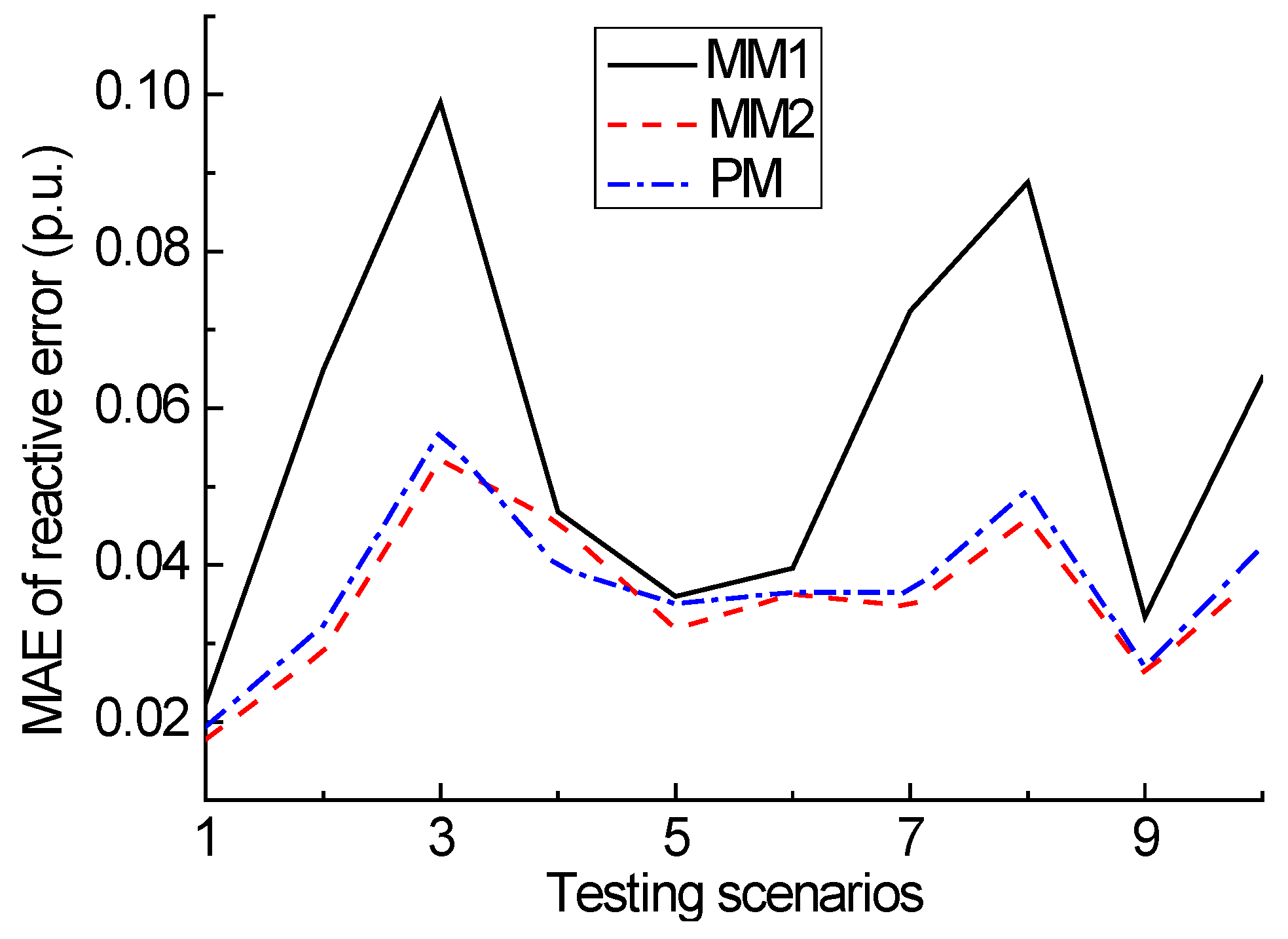
As shown in Table 2 and Figure 5, for the pre-fault phase ($t_0-1s,t_0$), the PM constructed in this paper exhibited higher active power simulation accuracy except in Case 6. In this phase, the active power output of the WF is stable. Moreover, the performance difference of the two mechanism models is relatively fixed for different scenarios. It helps to improve the accuracy of the PM through the optimal configuration of weight coefficients. For the other four phases, the improvement in accuracy decreased slightly, and the accuracy of the PM was between the MM1 and MM2 in some scenarios. The reason lies in that the active power output of WF starts to fluctuate in those phases, and the performance difference of the two mechanism models also begins to change in different scenarios. However, taking the quasi-steady-state phase during the fault $(t_0+0.14s, t_1)$into account, where the phenomenon that the accuracy of the PM is between the MM1 and MM2 appears more often, the active power errors of each model are presented in Figure 7. It can be seen that the active power performance of the PM is more stable than that of the MM1 and MM2, indicating its better adaptability.

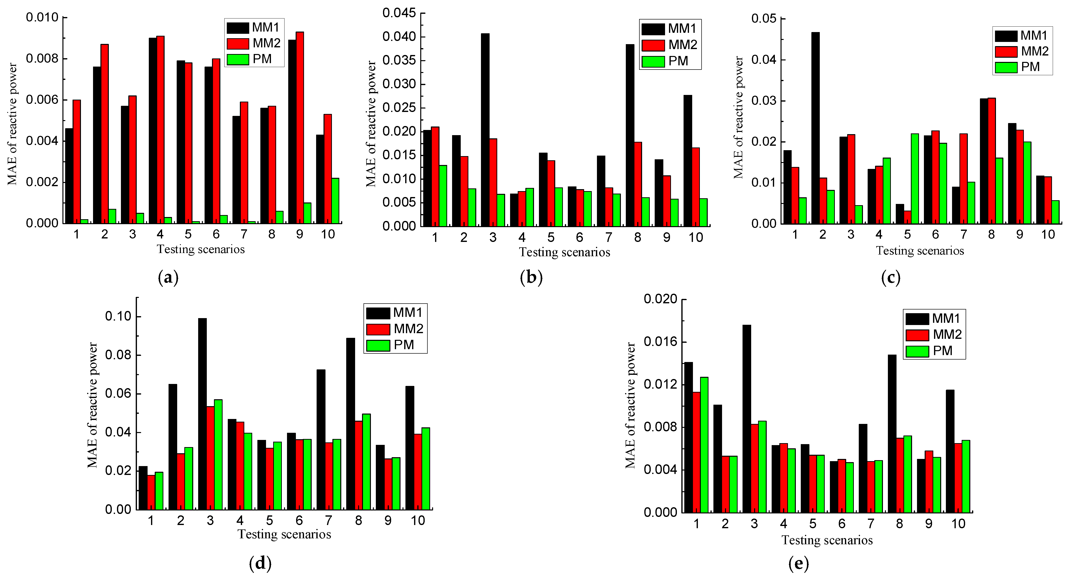
As shown in Table 3 and Figure 6, for the pre-fault phase ($t_0-1s,t_0$), the PM established in this paper also shows higher reactive power simulation accuracy. For the other four phases, the reactive power performance of the PM is between MM1 and MM2 in some scenarios. However, taking the early fault recovery phase into account, where the above phenomenon appears more often, the reactive power errors of each model are illustrated in Figure 8. It can be seen that the reactive power performance of the PM is also more stable.

To further demonstrate the effectiveness of the PM, the dynamic responses of the DM, PM, MM1 and MM2 in Cases 6 and 3 are presented in Figure 9 and Figure 10, respectively. As mentioned above, for Case 6, the accuracy of the PM was lower than both the MM1 and MM2. From Figure 9, we can observe that the PM remains accurate and has high correspondence with the electromechanical transient responses of the DM. For the other nine cases, for example, Case 3, it can be seen that the responses of the PM were much closer to that of the DM than the MM1 and MM2, as shown in Figure 10.

5. Discussion

Until now, the general equivalent modeling method for DFIG-based WFs has not been considered from a model-data driven point of view; only a few researchers have analyzed the possibility of identifying the crowbar action based on a data-driven model [31]. This means that the accuracy of WF-equivalent models has been improved, only considering coherent cluster divisions without regard to the adaptability of the equivalent model for different scenarios.

One of the novelties presented in this paper is to enhance the stable performance of WF-equivalent models in uncertain operating scenarios. As the scenario changes, the accuracy of the traditional WF equivalent models will also change, and the performance is often uncertain due to complex influencing factors. As shown in Figure 5 and Figure 6, sometimes the performance of the MM1 is better, and sometimes the performance of the MM2 is better. It is not clear in which scenario the effectiveness of the equivalent model will fail. Therefore, in the view of enhancing the stability of the model performance, we used data-driven mining of complementary characteristics between mechanism models. As shown in Figure 7 and Figure 8, the applicability to uncertain scenarios was significantly improved.

In addition, this paper provides meaningful insights into how to select mechanism models. We analyze the influence of the two calculation methods for the aggregated parameters of the collector cable on the accuracy of the equivalent model, and select two equivalent models with complementary characteristics. This helps to improve the accuracy of the general equivalent model. From Table 2 and Table 3, we can observe that except in rare phases, the accuracy of the general equivalent model is smaller than the maximum error between the two mechanism models. Moreover, the average error of the general equivalent model is also smaller than those of the two mechanism models.

The simulations were carried out on a workstation with the following specifications: Intel Xeon(R) Platinum 8375C, 32 CPU @ 2.9 GHz, 128 GB of RAM. The average simulation times of the DM, PM, MM1 and MM2 were 2146 s, 283 s, 135 s and 135 s, respectively. By the PM, the simulation time of the detailed WF can be significantly reduced by about 87 %. Compared to the MM1 and MM2, about two times the simulation time is increased.

6. Conclusions

From the viewpoint of improving the applicability and engineering utility value of the DFIG-based WF equivalent model, this paper proposes a general model-data-driven equivalent modeling method. It verifies the effectiveness of the proposed model for uncertain operation scenarios through simulation.

The two mechanism models are selected based on clustering indicators and calculation methods for the aggregated parameters of the collector cable. The combination of the two models can not only take advantage of the high accuracy of each model, but also take advantage of their complementary nature to reduce simulation errors.

In this paper, the fault process is divided into five stages, and the data-driven adaptive weight optimization model is constructed to optimize the corresponding weight coefficients. It further improves the adaptability of the general WF equivalent model in uncertain scenarios.

However, the main drawback of this general equivalent modeling method is that the accuracy of the PM is sometimes between the MM1 and MM2. In future works, a possible extension could be to apply the time series analysis theory to analyze the fluctuation law of the dynamic responses, and we will further improve the accuracy of the general equivalent model by optimizing the time window division.

References

- Haces-Fernandez, F.; Cruz-Mendoza, M.; Li, H. Onshore wind farm development: Technologies and layouts. Energies 2022, 15, 2381. [Google Scholar] [CrossRef]
- Council GWE. GWEC Global Wind Report 2022; Global Wind Energy Council: Bonn, Germany, 2022; pp. 119–125. [Google Scholar]
- Agarala, A.; Bhat, S.; Mitra, A.; Zycham, D.; Sowa, P. Transient stability analysis of a multi-machine power system integrated with renewables. Energies 2022, 15, 4824. [Google Scholar] [CrossRef]
- Skibko, Z.; Hołdynski, G.; Borusiewicz, A. Impact of wind power plant operation on voltage quality parameters—Example from Poland. Energies 2022, 15, 5573. [Google Scholar] [CrossRef]
- Cárdenas, B.; Swinfen-Styles, L.; Rouse, J.; Garvey, S.D. Short-, medium-, and long-duration energy storage in a 100% renewable electricity grid: A UK case study. Energies 2021, 14, 8524. [Google Scholar] [CrossRef]
- Fernández, L.M.; García, C.A.; Saenz, J.R.; Jurado, F. Equivalent models of wind farms by using aggregated wind turbines and equivalent winds. Energy Convers. Manag. 2009, 50, 691–704. [Google Scholar] [CrossRef]
- Zou, J.; Peng, C.; Yan, Y.; Zheng, H.; Li, Y. A survey of dynamic equivalent modeling for wind farm. Renew. Sustain. Energy Rev. 2014, 40, 956–963. [Google Scholar] [CrossRef]
- Han, J.; Li, L.; Song, H.; Liu, M.; Song, Z.; Qu, Y. An equivalent model of wind farm based on multivariate multi-scale entropy and multi-view clustering. Energies 2022, 15, 6054. [Google Scholar] [CrossRef]
- WECC Renewable Energy Modeling Task Force. WECC Wind Power Plant Dynamic Modeling Guidelines; ESIG: Reston, VI, USA, 2014. [Google Scholar]
- Chao, P.; Li, W.; Liang, X.; Xu, S.; Shuai, Y. An analytical two-machine equivalent method of DFIG-based wind power plants considering complete FRT processes. IEEE Trans. Power Syst. 2021, 36, 3657–3667. [Google Scholar] [CrossRef]
- Wu, Y.K.; Zeng, J.J.; Lu, G.L.; Chau, S.W.; Chiang, Y.C. Development of an equivalent wind farm model for frequency regulation. IEEE Trans. Ind. Appl. 2020, 56, 2360–2374. [Google Scholar] [CrossRef]
- Akhmotov, V.; Knudsen, H. An aggregate model of a grid-connected, large-scale, offshore wind farm for power stability investigations—Importance of windmill mechanical system. Int. J. Electr. Power Energy Syst. 2002, 24, 709–717. [Google Scholar] [CrossRef]
- Brochu, J.; Larose, C.; Gagnon, R. Validation of single- and multiple-machine equivalents for modeling wind power plants. IEEE Trans. Energy Convers. 2011, 26, 532–541. [Google Scholar] [CrossRef]
- Teng, W.; Wang, X.; Meng, Y.; Shi, W. Dynamic clustering equivalent model of wind turbines based on spanning tree. J. Renew. Sustain. Energy 2015, 7, 063126. [Google Scholar] [CrossRef]
- Zhou, Y.; Zhao, L.; Matsuo, I.B.M.; Lee, W.J. A dynamic weighted aggregation equivalent modeling approach for the DFIG wind farm considering the Weibull distribution for fault analysis. IEEE Trans. Ind. Appl. 2019, 55, 5514–5523. [Google Scholar] [CrossRef]
- Jin, Y.; Wu, D.; Ju, P.; Rehtanz, C.; Wu, F.; Pan, X. Modeling of wind speeds inside a wind farm with application to wind farm aggregate modeling considering LVRT characteristic. IEEE Trans. Energy Convers. 2020, 35, 508–519. [Google Scholar] [CrossRef]
- Zhu, Q.; Ding, M.; Han, P. Equivalent modeling of DFIG-based wind power plant considering crowbar protection. Math. Probl. Eng. 2016, 2016, 8426492. [Google Scholar] [CrossRef]
- Wu, Z.; Cao, M.; Li, Y. An equivalent modeling method of DFIG-based wind farm considering improved identification of Crowbar status. Proc. CSEE 2022, 42, 603–614. [Google Scholar]
- Zhu, Q.; Ding, M. Equivalent modeling of PMSG-based wind power plants considering LVRT capabilities: Electromechanical transients in power systems. SpringerPlus 2016, 5, 2037. [Google Scholar]
- Kunjumuhammed, L.P.; Pal, B.C.; Qates, C.; Dyke, K.J. The adequacy of the present practice in dynamic aggregated modeling of wind farm systems. IEEE Trans. Sustain. Energy 2017, 8, 23–32. [Google Scholar] [CrossRef]
- Wang, Z.; Yang, G.; Tang, Y.; Cai, W.; Liu, S.; Wang, X.; Ouyang, J. Modeling method of direct-driven wind generators wind farm based on feature influence factors and improved BP algorithm. Proc. CSEE 2019, 39, 2604–2614. [Google Scholar]
- Ma, Y.; Runolfsson, T.; Jiang, J.N. Cluster analysis of wind turbines of large wind farm with diffusion distance method. IET Renew. Power Gener. 2011, 5, 109–116. [Google Scholar] [CrossRef]
- Ali, M.; Ilie, I.S.; Milanović, J.V.; Chicco, G. Wind farm model aggregation using probabilistic clustering. IEEE Trans. Power Syst. 2013, 28, 309–316. [Google Scholar] [CrossRef]
- Zhu, Q.; Han, P.; Ding, M.; Zhang, X.; Shi, W. Probabilistic equivalent model for wind farms based on clustering-discriminant analysis. Proc. CSEE 2014, 34, 4770–4780. [Google Scholar]
- Zhou, H.; Ju, P.; Xue, Y.; Zhu, J. Probabilistic equivalent model of DFIG-based wind farms and its application in stability analysis. J. Mod. Power Syst. Clean Energy 2016, 4, 248–255. [Google Scholar] [CrossRef]
- Zhu, Q. Research on Equivalent Modeling of Wind Farm for Electromechanical Transient Stability Analysis. Ph.D. Thesis, Hefei University of Technology, Hefei, China, 2017. [Google Scholar]
- Muljadi, E.; Butterfield, C.P.; Ellis, A.; Mechenbier, J.; Hochheimer, J.; Young, R.; Miller, N.; Delmerico, R.; Zavadil, R.; Smith, J.C. Equivalencing the collector system of a large wind power plant. In Proceedings of the 2006 IEEE Power Engineering Society General Meeting, Montreal, QC, Canada, 18–22 June 2006; pp. 1–9. [Google Scholar]
- Zou, J.; Peng, C.; Xu, H.; Yan, Y. A Fuzzy clustering algorithm-based dynamic equivalent modeling method for wind farm with DFIG. IEEE Trans. Energy Convers. 2015, 30, 1329–1337. [Google Scholar] [CrossRef]
- Lee, D.; Son, S.; Kim, I. Optimal allocation of large-capacity distributed generation with the volt/var control capability using particle swarm optimization. Energies 2021, 14, 3112. [Google Scholar] [CrossRef]
- IEC 61400-27-1:2015; Wind Turbines—Part 27-1: Electrical Simulation Models—Wind Turbines. IEC: Geneva, Switzerland, 2015.
- Wu, L.; Chao, P.; Li, G.; Li, W.; Li, Z. Hybrid data-model-driven aggregation equivalent modeling method for wind farm. Autom. Electr. Power Syst. 2022, 46, 66–74. [Google Scholar]
Figure 1.
Framework of general equivalent modeling method.
Figure 2.
Training database construction flowchart.
Figure 3.
DFIG-based WF topology.
Figure 4.
Ten test scenarios. (a) Wind speed scenarios. (b) Voltage dip scenarios.
Figure 5.
Active power response error of three equivalent models. (a) Pre-fault phase. (b) Early fault phase. (c) Quasi-steady-state phase during the fault. (d) Early fault recovery phase. (e) Quasi-steady-state phase during the fault recovery.
Figure 6.
Reactive power response error of three equivalent models. (a) Pre-fault phase. (b) Early fault phase. (c) Quasi-steady-state phase during the fault. (d) Early fault recovery phase. (e) Quasi-steady-state phase during the fault recovery.
Figure 7.
Active power errors of different models in quasi-steady-state process during fault duration.
Figure 8.
Reactive power errors of different models in quasi-steady-state process during fault duration.
Figure 9.
The dynamic responses of WF at POC in Case 6. (a) Active power. (b) Reactive power. (c) Voltage.
Figure 10.
The dynamic responses of WF at POC in Case 3. (a) Active power. (b) Reactive power. (c) Voltage.