Machine Learning Analysis on the Performance of Dye-Sensitized Solar Cell—Thermoelectric Generator Hybrid System

Abstract

In cases where a dye-sensitized solar cell (DSSC) is exposed to light, thermal energy accumulates inside the device, reducing the maximum power output. Utilizing this energy via the Seebeck effect can convert thermal energy into electrical current. Similar systems have been designed and built by other researchers, but associated tests were undertaken in laboratory environments using simulated sunlight and not outdoor conditions with methods that belong to conventional data analysis and simulation methods. In this study four machine learning techniques were analyzed: decision tree regression (DTR), random forest regression (RFR), K-nearest neighbors regression (K-NNR), and artificial neural network (ANN). DTR algorithm has the least errors and the most R², indicating it as the most accurate method. The DSSC-TEG hybrid system was extrapolated based on the results of the DTR and taking the worst-case scenario (node-6). The main question is how many thermoelectric generators (TEGs) are needed for an inverter to operate a hydraulic pump to circulate water, and how much area is required for that number of TEGs. Considering the average value of the electric voltage of the TEG belonging to node-6, 60,741 pieces of TEGs would be needed, which means about 98 m² to circulate water.

1. Introduction

Current demand for energy consumption, and for reliable and resilient energy systems are based on burning fossil fuels [1]. The need for energy is undisputedly one of the most important questions for researchers and engineers. The previous century’s energy generation methods are recognized as unsuitable, due to increasing carbon-dioxide (CO₂) emission into the atmosphere [2]. The outstanding role of non-renewable energy sources cause environmental concerns because they emit greenhouse gases into the environment which lead to serious health and environmental repercussions [3]. Renewable energy resources have been growing and receiving significant attention all around the world because they are widely available, non-polluting and clean [4]. Renewable energy resources such as wind, sun, hydro, geothermal and biomass are expected to take over the dominant role of the global electricity generation and become the largest energy resource by 2030 [5]. Photovoltaics among the renewables have gained the highest growth rate during the last few decades. Presently, wind generates more electrical energy than photovoltaic (PV), however, wind-turbines are very site specific, and PV is applicable to most locations [5]. On the other hand, photovoltaics has emerged as a promising solution in the battle against global climate change.

Amongst various solar cells, the dye-sensitized solar cell (DSSC) belongs to the third-generation of solar cells, and it is considered a promising, forward-looking solar cell device because of its low-cost, ease of production, affordability and environmentally friendliness [6]. In addition, the perovskite solar cell (PSC) is also a third-generation solar cell the great advantages of which are it’s higher absorption coefficient and more efficient hole transport compared to DSSC [7,8]. DSSC is also a light harvester that converts light energy into electrons, just as other types of solar cells do, but with a difference in the working principle. In the case of silicon (Si) based solar cells, the semiconductor layer absorbs and divides the charge carrier, while in the case of DSSCs the absorption and division are completed separately [9].

The above-mentioned factors make DSSC more attractive in a wide range of applications; in architecture, for instance, where it is used as a building integrated solar cell [10]. However, photovoltaics has achieved enormous progress and the research background is undoubtedly grounded, issues regarding their relatively low energy harvesting efficiency (including DSSC) remain unsolved because of their disability to exploit the solar spectrum in a wide range [11]. Although, many studies have attempted to improve the structure of the n-type semiconductor layer of DSSC or to develop new dye to increase the energy harvesting efficiency, according to the DSSC trends, the efficiency only increases with a small gradient [12]. On the other hand, when the DSSC device is exposed to sunlight, the sunlight radiation makes the surface and inside temperature of the DSSC rise and generate heat energy [13]. This phenomenon occurs because the panchromatic absorber absorbs photons in the visible and near-infrared region, with the result that the absorption range is limited. Thus, photons of a longer wavelength are dissipated as heat energy. It is considered that more than 40% of the incident solar energy is converted into heat energy [14]. The inside accumulated thermal energy has a reduction effect on the solar cell and influences the maximum power and efficiency of the DSSC decreasingly [15]. If the accumulated heat is transported and then transformed into electricity, the overall maximum power and efficiency of the DSSC can be increased. Otherwise, the undesired heating process can damage the structure of the light-harvesting material via photochemical degradation and thermal stress [14]. The device, which converts thermal energy into electrical current via the Seebeck effect is the thermoelectric generator (TEG). The combination of PV and TEG forms a hybrid system and can improve the overall efficiency. Moreover, utilizing the thermal energy accumulated inside the DSSC is a useable approach. TEGs consist of p- and n-type semiconductor thermoelements electrically connected in series and inserted between two electrically insulated ceramic plates [16]. Taking into consideration that the device’s working principle is based on the Seebeck effect, a high temperature difference between the two ceramic plates could generate high electrical current. The choice of materials for thermoelements determine the amount of extractable electrical current. However, though high-temperature materials, such as lead telluride (PbTe) or silicon-germanium (SiGe), have arrived in the market, bismuth telluride (BiTe) has become relatively cheap and favorable for thermoelectric generator [17].

Research dealing with a PV–TEG hybrid system was first reported in the 1970s and most of the work has focused on silicon solar cells. During the last decades, emerging PV technologies (DSSC) hybridized with TEG have been reported [14]. In the literature, only a limited number of papers are available that deal with the performance of a dye-sensitized solar cell thermoelectric generator hybrid system. Kossyvakis et al. examined the performance of polycrystalline silicon (poly–Si) and DSSC hybrid solar cells. It is stated that in the case of a poly–Si solar cell higher power output is obtained, however, DSSC could become attractive when the incorporation of solar cells in PV–TEG hybrids operate at elevated temperatures [18]. Guo et al. developed and tested a two-compartment DSSC–TEG hybrid cell. The efficiency of the system increased 10% compared to an individual DSSC [19]. Wang et al. presented a pioneering work in which they combined a DSSC, a solar selective absorber and a TEG into a hybrid device. Although, the device was not optimized, the overall efficiency could reach 13% [20]. Chang et al. used a nano-copper thin film as a medium of thermal conductivity to improve the heat transfer between DSSC and TEG. In the testing environment the intensity of the simulated sunlight was 100 mW/cm² and their results show that the device could produce 4.97 mW/cm² power, increasing the output by 2.87% when compared to employing the DSSC alone [21]. Another system composed by Chang et al. integrated pulsating heat pipes to a DSSC–TEG system in order to improve the overall efficiency. Using a simulated light source, the power output of the thermoelectric module reached 11.48 mW/cm² [22]. Su et al. presented an experimental and analytical study about DSSC–TEG performance. The temperature effect on the performance of the device was also discussed [23]. Kim et al. structured and built a DSSC–TEG hybrid generator in which the electron recombination lifetime was increased by the TEG [24].

Table 1. An overview of the recent work on a dye-sensitized solar–thermoelectric generator hybrid cell. The dimension of the power density is mW/cm².

Literature	Author	Year	Comments	Power Density	Location	Model
[18]	Kossyvakis et al.	2016	Examined the performance of poly–Si–TEG hybrid and DSSC–TEG hybrid cells. According to the results, higher efficiency was achieved using poly–Si–TEG hybrid cells.	1	Indoor	Experimental
[19]	Guo et al.	2010	Presented a two-component DSSC–TEG hybrid cell resulting in a 10% increase in system efficiency.	2.5	Indoor	Experimental
[20]	Wang et al.	2011	Utilized a wider part of the solar spectrum using a solar selective absorber and TEG. The overall conversion efficiency of the built and tested hybrid system was larger than 13%.	n/a	Indoor	Experimental
[25]	Chang et al.	2010	Coated the TEG surface with self-prepared CuO thin film which elevated the surface temperature of the TEG by 2 °C and the generated voltage by 14.8%, increasing the overall efficiency by 10% and the power output by 2.35%. The overall generated power output was about 4.95 mW/cm2.	4.95	n/a	Experimental
[22]	Chang et al.	2012	Integrated pulsating heat pipes to DSSC–TEG hybrid system to increase the power output. The power output of the thermoelectric modules was 11.48 mW/cm2.	11.48	Indoor	Experimental
[23]	Su et al.	2014	The effects of the operating electric current, working temperature and temperature dependent coefficient in the DSSC on the performance of the hybrid device are discussed.	4.95	n/a	Analytical
[24]	Kim et al.	2020	Designed and built a DSSC–TEG hybrid cell in which the electron recombination lifetime is increased because of the TEG device-	10.8	Indoor	Experimental and Analytical

shows the overview of the recent work on a DSSC–TEG hybrid cell with their locations (indoor or outdoor) and the model (experimental, analytical or machine learning).

According to the studied literature, the tests were run and results taken in laboratory environments using simulated sunlight (usually 100 mW/cm²) and not in outdoor conditions. Moreover, the results show that the overall output power and efficiency have increased using thermoelectric generator to recycle the waste heat from the system. Furthermore, the used methods belong to conventional data analysis and simulation methods. These methods are undoubtedly important; however, machine learning (ML) has recently made an outstanding influence on the energy sector by discovering hidden patterns and identifying correlations between an input object and the desired output value [26]. This black-box approach is unattainable using traditional methods [27,28]. Among ML regression methods, many algorithms can be found, of which decision tree (DT), random forest (RF), K–nearest neighbor, and artificial neural network (ANN) are used.

A decision tree (DT) forms a tree structure, in which the dataset is broken into subsets resulting in a tree with decision nodes and leaf nodes. Conclusions can be deducted based on the categorized responses that are represented in the leaf nodes. The root node of the tree is the parent node of all existing nodes, where each link represents a decision, and each leaf represents an outcome [29]. A random forest (RF) algorithm is an extension of the bagging method, which assembles decision trees which are uncorrelated [30]. RF trains a collection of trees and adds randomness at different levels (e.g., random sampling for each tree) [31]. It is worth mentioning that the difference between a decision tree and a random forest is that, while a DT considers all the possible feature divisions, an RF selects a subset of those features [32]. A K–nearest neighbor is a simple non-parametric approach to machine learning. The advantage of this method is that it can also be used for classification and regression [33]. The artificial neural network algorithm has also received a great deal of attention among ML methods and can also be used for both data classification and performance prediction. The ANN algorithm involves training and test procedures, through which weights and biases are shaped to minimize the errors in target prediction. A typical ANN consists of three layers: the input layer, hidden layer and output layer [34]. Taking advantage of the machine learning methods in DSSC–TEG hybrid system research, the current study paves the path to outstanding results and provides some key insight related to this field.

To address the above-mentioned challenges, the present research aims to apply machine learning regression algorithms based on experimental data to predict the performance, known as maximum power output, of the DSSC–TEG hybrid system in outdoor summer conditions. Outdoor experiments were planned and conducted on the basis of laboratory measurements and dependent and independent variables were selected. In addition, decision tree regression, random forest regression, K–nearest neighbor regression, and artificial neural network algorithms were successfully used.

2. Materials and Methods

2.1. Experimental Setup

2.1.1. Materials: Dye-Sensitized Solar Cell and Thermoelectric Generator

For the purpose of the present work, a commercial dye-sensitized solar cell (Ref. number: 51201) was purchased from Solaronix Ltd. The size of the manufactured DSSC is 25 mm × 25 mm. In order to implement the construction of the experimental setup, a thermoelectric generator known as a commercial TEC1-12715 was purchased from Hestore Ltd. The device consists of 127 thermocouples and the area is 40 mm × 40 mm × 3.8 mm. The internal resistance of the TEG is 5 $\mathsf{\Omega }$. The material of the thermoelectric generator is BiSn which is commonly used material for TEGs, and it is also regarded as an appropriate thermoelectric material. A hydraulic pump (Eden 114) was inserted to circulate the water in the cooling system. Initially, the performance of the DSSC and the TEG were tested before laboratory and outside conditions.

2.1.2. Assembling and Testing of the PV–TEG Hybrid System

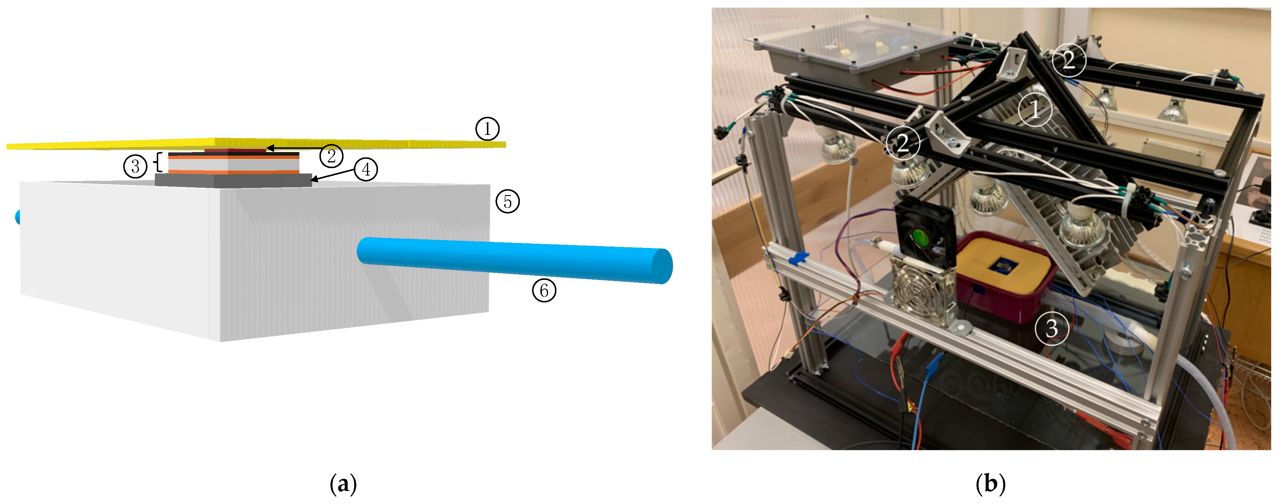
In order to experimentally investigate the DSSC–TEG hybrid system, a sandwich-like target system was designed and tested. Figure 1a shows the 3D drawing of the structure of the sandwich-like target system in a water bath (shown as number 5) where the blue cylinder (shown as number 6) is the water pipe. A black painted aluminum plate (shown as black rectangle as part of the number 3) was attached between the DSSC (shown as number 2) and the TEG (shown as white rectangle as part of the number 3) to improve the emission or absorption ability. A thin layer of thermal grease (shown as orange rectangle as part of the number 3) (Arctic MAX-4 2019, thermal conductivity 8.5 W/mK [35]) enhanced the thermal conductivity and provided the contact uniformity between the aluminum plate and thermoelectric generator, and between the thermoelectric generator and the aluminum heat sink (shown as number 4). As a result, the exhausted heat can be recycled efficiently. The dimensions of the aluminum heat sink are 70 mm by 45 mm by 75 mm for the width, height, and length. To induce a high temperature gradient between the two sides of the TEG, in other words to facilitate the release of heat, a water cooling technique was applied, which means that the aluminum heat sink was immersed in a water bath, where water flows. The applied cooling technique was investigated and introduced in [35]. Thermal couples were attached to the hybrid system to measure the temperature of the surface of the DSSC and the temperature difference between the hot side and the cold side of the thermoelectric generator. Meanwhile, taking the high heat transport originating from the device into consideration a thermal insulator, extruded polystyrene (known as XPS) (shown as number 1), was installed (see in Figure 1a,b).

It can be seen that the surface of the DSSC is smaller than the surface of the TEG. The reason of this phenomena is that, in this experiment, very cheap commercially available TEG was purchased and was used which was also the smallest size compared to other purchasable TEGs. Separate indoor tests with fixed light intensity and temperature were needed to reveal the efficiency of the water-cooling technique. Subsequently, measurements took place in a laboratory environment using artificial light sources to measure the electric current–voltage characteristics of the DSSC and the electrical voltage of the TEG. A sun simulator was built that employed a light emitting diode (LED) (shown as number 1 in Figure 1b) and halogen lamps (shown as number 2 in Figure 1b). The sun simulator device was constructed based on [36]. Figure 1b shows the built sun simulator device with the built and tested target system (shown as number 3) in a water bath. During the entire experiment, the cold side of the thermoelectric generator was a constant 20 °C ± 1.5 °C. After carrying out the measurements, a conventional statistical method (one-way ANOVA) was used to examine the performance of the built DSSC–TEG hybrid system and to check how the system matches with the results reported in the above-mentioned scientific works.

In order to assess the experimental data, the power of the DSSC was extrapolated or, in other words, was multiplied by four. The overall power output is the sum of the extrapolated maximum power point of the DSSC, and the power of the TEG, which was calculated from the measured voltage using the following equation:

$$P=\frac{V_{CC}^2}{R_L}$$

(1)

where $V_{CC}$ is the closed-circuit voltage over the resistance load $\left(R_L\right)$. The value of the resistance was $R_L=10 \mathsf{\Omega }$. The experiment involved n = 30 tests and, based on the description statistics and homogeneous test, a probe was selected. Due to the violation of the normality (the maximum absolute value of skewness is 1.444 and the maximum absolute value of kurtosis is 1.428) and the violation of Levene’s test (F (6203) = 13.771, p < 0.001), a Welch probe was applied. Based on the Welch probe (F (6,86.131) = 12,750.2, p < 0.001), there was a significant relationship between the temperature and the maximum power output of the DSSC–TEG hybrid system, and the ${\eta }_p^2=0.996$. Moreover, a Bonferroni post-hoc test was used, and results show that there is a significant difference between every measured (30, 34, 35, 37, 40 and 43 °C) temperature.

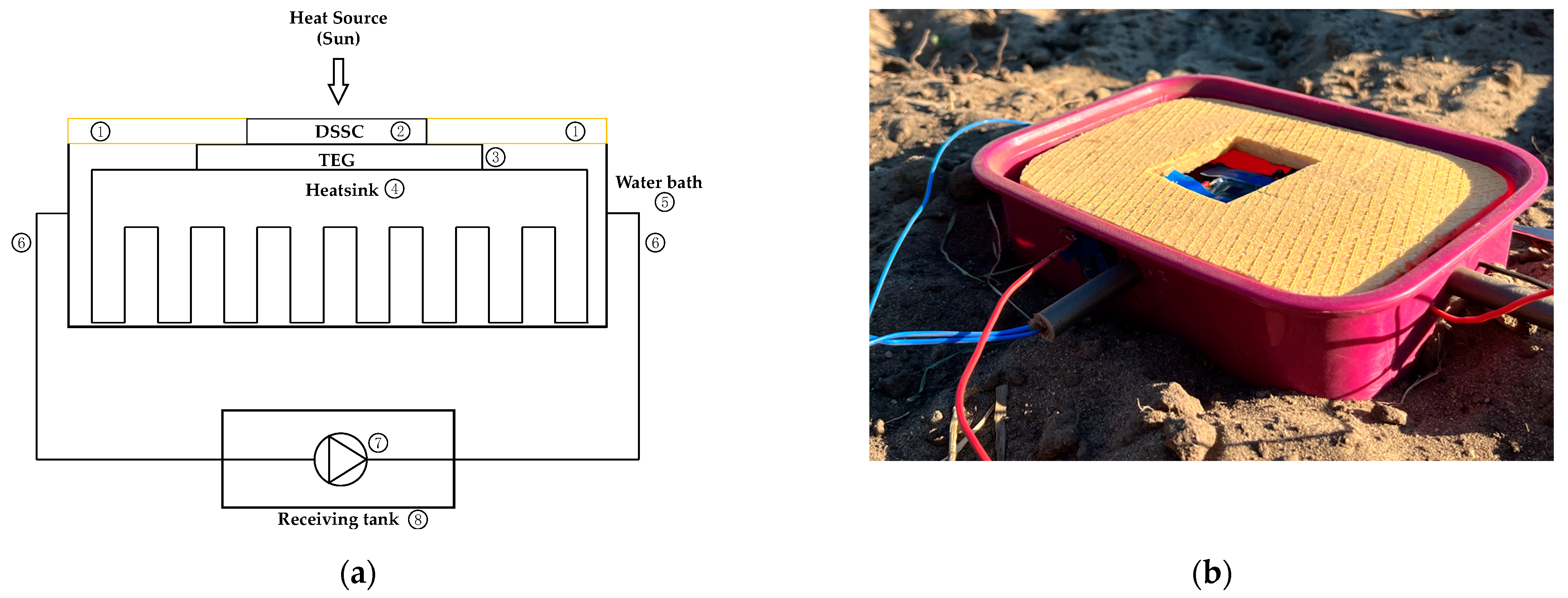
According to the laboratory tests, the built DSSC–TEG hybrid system works as in the reported literature. To get the real performance correct, it is important to complement laboratory measurements with outdoor tests. On the basis of laboratory tests, outdoor measurements were taken in Hungary (47.433083° N, 18.591398° E) during the middle of summer. The same water-cooling technique was used as in the laboratory environment. Therefore, an isolated box was placed 1.5 m deep in the ground to maintain a constant temperature to the cold side of the TEG. The excavated depth was considered to be appropriate because the water pipes which supply the water between the driven well and the house, are placed at such a depth. The installed sensors were an irradiation sensor (Steca TA ES1), to record the solar irradiation and a K-type thermocouple (Voltcraft K204) to measure cell temperature, and the two sides of the thermoelectric generator. The radiometer was positioned in the same angle as the system. To measure the voltage, a Picolog 1216 data logger was used. Figure 2a) shows the schematic overview of the target system and Figure 2b) represents the built and tested DSSC–TEG hybrid system during the outside experiment with the cables, which were used to measure the target parameter and the predictor parameters.

2.2. Principles of Chosen Machine Learning Techniques (Methods)

Regression models, which are supervised learning, were implemented using JASP software. Furthermore, the target parameter is the overall power output of the DSSC–TEG hybrid system, the predictors are the temperature difference between the sides of the TEG, the irradiation intensity, and the surface temperature of the DSSC.

The software differentiates supervised and unsupervised learning methods. For supervised methods regression and classification methods can be used. Nevertheless, the target (the overall maximum power output of the DSSC–TEG hybrid system) is continuous, regression methods were used to model the relations. Four machine learning (ML) techniques were analyzed: decision tree regression, random forest regression, K-nearest neighbors regression, and artificial neural network (ANN).

2.2.1. Decision Tree Regression

A decision tree is a hierarchical tree structure which consists of a root node, branches, internal nodes (known as decision nodes), and leaf nodes. It starts with a root note which is the parent of all existing sub-nodes, and does not have any incoming branches. Furthermore, the branches (links) expand from the root node into the internal nodes by breaking down the dataset into smaller and smaller subsets [37]. A decision node (or internal node) has two or more branches, each representing values for the attribute tested. Leaf nodes represent the possible outcomes from which conclusions can be deducted [38]. A decision tree algorithm uses an iterative process, a greedy search, in which the data splitting into partitions is undertaken by minimizing the sum of squared deviations from the mean in the two separate partitions [29]. There are different types of decision tree algorithms, including popular ones such as iterative dichotomiser 3 (ID3), a later iteration of ID3 (C4.5), and classification and regression trees (CART) [29]. In this work, the CART algorithm was used for data evaluation and for predictions. For the predictions, data (total: 106) were divided into training and test data: 80% of the data (train: 85) were used for the training of the model, and 20% of the data (test: 21) were used for testing purposes. The percentage of the test data only tells the size of the partition, so the test data were randomly selected by the software.

2.2.2. Random Forest Regression

A random forest algorithm is a set of parallel decision trees, which are relatively weak classifiers and uncorrelated. It utilizes bagging and feature randomness to generate a random subset of features. The algorithm works by generating trees which have their own individual prediction, and then averaging the predictions of the individual trees to produce a single result [32]. A random forest is a useful algorithm because it avoids overfitting (reduced risk of overfitting) which can come up in case of a decision tree algorithm [39], and is able to cope with non-linear relationships. The used software splits the data into train, test, and validation data for predictions. The split is randomly undertaken by the software. Of the overall data, 20% are test data, the other 20% are for validation, and the rest are the training data.

2.2.3. K-Nearest Neighbors Regression

K-nearest neighbors (K-NN) regression is an instance-based learning, which is the most elementary and easy to implement non-parametric regression approach used in machine learning. The basis of the K-NN regression algorithm can be defined in three major steps: (i) computing the predefined distance between the testing and the training data set; (ii) defining k with a minimum distance from the training data set; and (iii) predicting the power output of the DSSC–TEG hybrid system on the basis of a weighted averaging approach [40]. In order to calculate the distance between the testing data set and the training data set Euclidean, Manhattan, Minkowski, and Chebyshev functions can be used [41]. The Euclidean and Manhattan distance functions are widely used distance metrics [42]. In this research, Manhattan distance function was used.

2.2.4. Artificial Neural Network

An artificial neural network is one of the most frequently used machine learning algorithms. A typical architectural structure of an ANN consists of three layers: input layer, hidden layer, and output layer [30]. The artificial neurons, known as nodes, are connected, and receive, process, and transmit signals. The training processes by modifying the weight parameters of the network neurons, because each neuron has a weight function, called an activation function, that processes the input data [43]. Meanwhile, the linking functions define the data transmission between nodes. Nevertheless, the outputs of the neurons in the output layer depend on the weight function of the neurons and the linking function between the nodes. The connected neurons in the network form a topology whose weights have be defined to minimize the error [32].

2.2.5. Evaluation Criterion

The performances of the used machine learning algorithms are compared to each other using five different metrics: mean squared error (MSE), root means squared error (RMSE), mean absolute error (MAE), mean absolute percentage error (MAPE) and coefficient of determination (R²).

Table 2. Evaluation metrics, description, equations, and performance criteria.

Metrics	Equation	Description	Performance Criteria
MSE	$\frac{1}{n} {\displaystyle {\displaystyle \sum }_{i=1}^n}{\left(x_i-y_i\right)}^2$	It is the mean of the squared prediction errors over all instances [44].	If the value is close to zero, the model is more successful [44].
RMSE	$\sqrt{\frac{1}{n} {\displaystyle {\displaystyle \sum }_{i=1}^n}{\left(y_i-x_i\right)}^2}$	It represents the difference between actual and estimated value [39].	It takes positive values and the closer the value is to zero, the more successful the estimation result is [39].
MAE	$\frac{1}{n} {\displaystyle {\displaystyle \sum }_{i=1}^n}\left|y_i-x_i\right|$	It represents the sum of absolute errors divided by the sample size [32].	As the value approaches zero, it indicates that the model is more accurate [32].
MAPE	$\frac{1}{n} {\displaystyle {\displaystyle \sum }_{i=1}^n}\left|\frac{x_i-y_i}{x_i}\right|·100$	It describes the success of the predictive model by measuring the size of the errors as a percentage [39].	The lower the value is (close to zero), the greater the performance of the model is [39]. Low precision: MAPE $>$ 50%; Reasonable precision: 20% $<$ MAPE $\le$ 50%; Good precision: 10% $<$ MAPE $\le$ 20%; Excellent precision: MAPE $\le$ 10%.
R2	$1-\frac{\sum {\left(y_i-x_i\right)}^2}{\sum {\left(x_i-\overline{x_i}\right)}^2}$	It represents how well the model predicts the actual data [43].	The value is between 0 and 1. The closer the value to 1, the better the forecast is [43].

MSE—mean squared error, RMSE—root mean square error, MAE—mean absolute error, MAPE—mean absolute percentage error, R²—coefficient of determination. The $y_i$ represents the data estimated by the models, the $x_i$ is the data obtained from the measurement stations, the $\overline{x_i}$ is the average of the measured data, and $n$ is the number of observations.

contains the evaluation metrics, equations, description, and performance criteria.

2.3. Data Preprocessing

After taking the outdoor measurements, data were gathered, and dependent and independent variables were selected. It is noteworthy that the connected weather parameters such as temperature and light intensity make the relations of the parameters and the maximum power output complicated to analyze using conventional linear models e.g., linear regression. Therefore, machine learning methods were used. The predictor parameters are the surface temperature of the dye-sensitized solar cell, the irradiation, and the temperature difference between the two sides of the thermoelectric generator. The target parameter is the overall maximum power output of the built DSSC–TEG hybrid system. As mentioned in the previous section, the experimental voltage data were recorded and saved by Picolog 1216 datalogger. Considering that the measurement is time dependent, a MatLab routine was developed to eliminate time and calculate the electric current using Ohm’s Law, which resulted in obtaining the electrical current–voltage data points (coordinates). On the other hand, because overlapping data points do not occur, smoothing procedures were not required. As a next step, the developed routine fits the simplified equation of the electric current–voltage characteristics of the solar cell:

$$y=a-b\left(e^{c·x}-1\right)$$

(2)

where a, b, and c are equation parameter constant. The fitted constants (a, b, and c), the maximum power point, and the quality of fit (r²) is determined and written into a file. The value of r² drops around 0.94, respectively, which is considered remarkable. Furthermore, data normalization and transformation were applied for the decision tree regression (DTR), random forest regression (RFR), and K-nearest neighbors regression (KNNR) methods. Thus, the scale data type was transformed into ordinary data type. For this preparation MatLab was used and the

Table 3. The applied data processing in order to transform the scale data type to ordinary data type in case of surface temperature of the dye-sensitized solar cell (T), intensity (Int) and temperature difference between the two sides of the thermoelectric generator (dT).

Ordinary Number	T	Dimension	Int	Dimension	dT	Dimension
0			0–100	W/m2	0–1	°C
1	0–25	°C	101–200	W/m2	1.1–2	°C
2	25.1–26	°C	201–300	W/m2	2.1–3	°C
3	26.1–27	°C	301–400	W/m2	3.1–4	°C
4	27.1–28	°C	401–500	W/m2	4.1–5	°C
5	28.1–29	°C	501–600	W/m2	5.1–6	°C
6	29.1–30	°C	601–700	W/m2	6.1–7	°C
7	30.1–31	°C	701–800	W/m2	7.1–8	°C
8	31.1–32	°C	801–900	W/m2	8.1–9	°C
9	32.1–33	°C	901–1000	W/m2	9.1–10	°C
10	33.1–34	°C	1001–1100	W/m2	10.1–11	°C
11	34.1–35	°C	1101–1200	W/m2	11.1–12	°C
12	35.1–36	°C	1201–1300	W/m2
13	36.1–37	°C
14	37.1–38	°C
15	38.1–39	°C
16	39.1–40	°C
17	40.1–41	°C
18	41.1–42	°C

T—surface temperature of the DSSC, Int—intensity, dT—temperature difference between the two sides of the thermoelectric generator.

. shows the transformation in the data.

3. Results

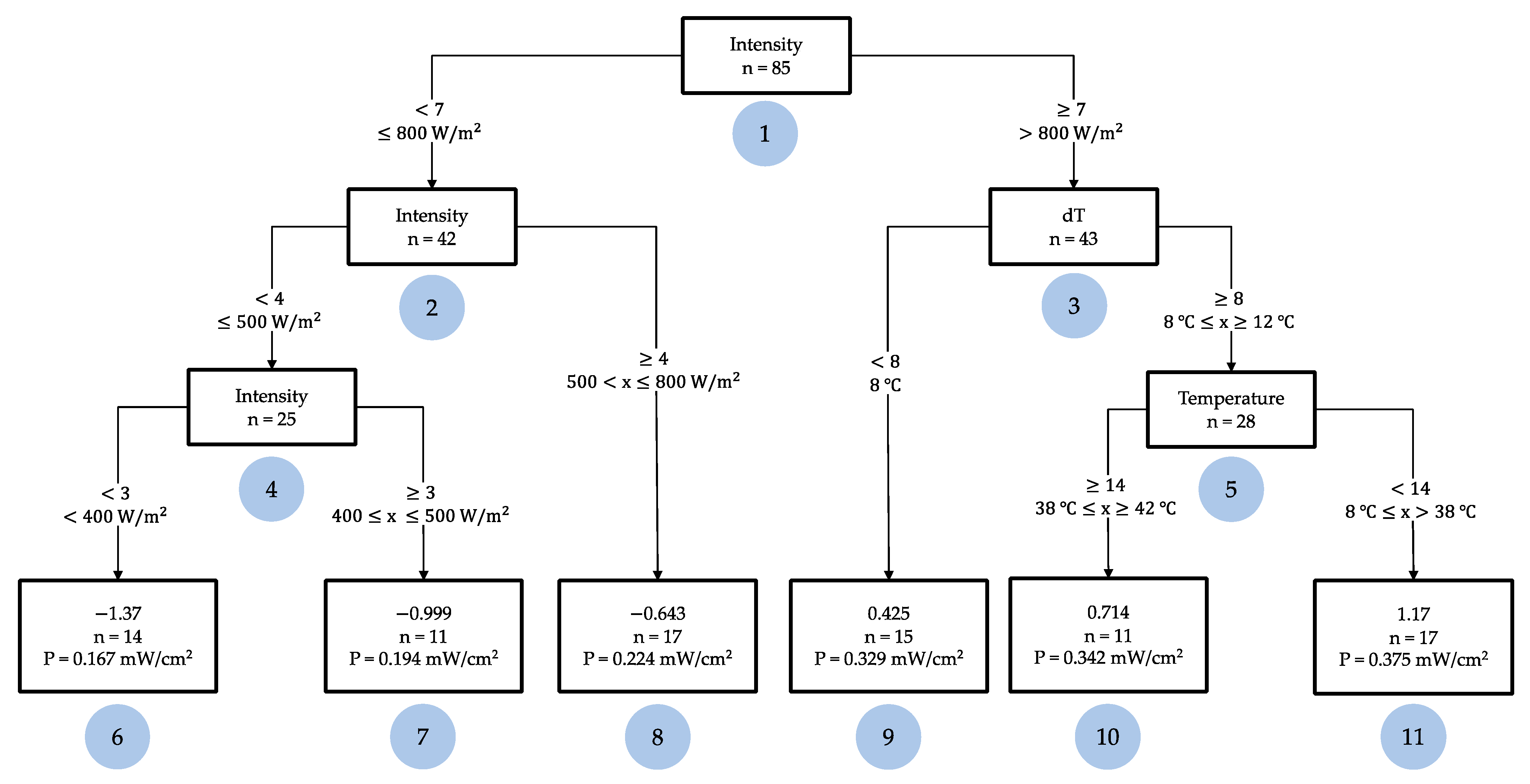
The current paper uses four different machine learning algorithms to predict the overall power output of the built DSSC–TEG hybrid system based on experimental data in outdoor summer conditions, located in Hungary. As mentioned above, four machine learning techniques were analyzed: decision tree regression, random forest regression, K–nearest neighbors regression, and artificial neural network. Figure 3 shows the decision tree model identifying the possible outcomes of the built DSSC–TEG hybrid system, and

Table 4. Evaluation table of the leaf nodes (node-6–11) of the decision tree where the dimensions are the following: P [mW/cm²], Int [W/m²], T [°C], dT [°C].

ID	Mean of P	Std of P	Mean of Int	Std of Int	Mean of T	Std of T	Mean of dT	Std of dT
6	0.1667	0.0206	288.133	65.3223	29.7	1.66	2.7	0.77
7	0.194	0.01	437.33	30.3535	31.7333	0.5132	2.9333	0.3786
8	0.2239	0.0366	575.7278	76.8788	22.9556	1.1758	4.6333	1.1792
9	0.329	0.0387	1006.4	91.1922	36.5875	2.5934	6.645	1.4137
10	0.3417	0.0228	1071.7	33.2467	39.57	0.868	8.44	0.6802
11	0.35752	0.0109	974.828	70.6193	35.52	0.8701	8.8	0.6519

Std—standard deviation, P—overall power output of the DSSC-TEG hybrid system, Int—intensity, T—surface temperature of the DSSC, dT—temperature difference between the two sides of the TEG.

represents the results of the decision tree regression model, including the mean of the overall power output of the DSSC–TEG hybrid system (Mean of P); the standard deviation of the power output (Std of P); the mean of the intensity irradiation (Mean of Int); the standard deviation of the intensity irradiation (Std of Int); the mean of the surface temperature of the DSSC (Mean of T); the standard deviation of the surface of the DSSC (Std of T); the mean of the temperature difference between the two sides of the TEG (Mean of dT); and the standard deviation of the temperature difference between the two sides of the TEG (Std of dT) to help better understand Figure 3 using the ID.

From Figure 3 it can be concluded that six leaf nodes are generated from the splits. The decision tree splits from the root node, which consists of 100% (n = 85) of the test data. The resulting root node, the four interior nodes and the six leaf nodes are represented with numbers under the nodes in blue circles. The first split was obtained by the intensity feature and resulted in two interior nodes: node-2 and node-3, and it is supported by results of the feature’s importance. Consequently, intensity has the greatest relative importance with 39.374 amongst the other features. According to the decision tree, the first leaf node (node-6) is obtained if Intensity is lower than 400 W/m². In this case, the mean of the overall power output of the built DSSC–TEG hybrid system is 0.167 mW/cm². Moreover, it can be seen that every part of the left sub-tree is divided only by intensity. Therefore, if Intensity is equal or lower than 800 W/m², then we can predict from the value of the intensity how much the overall power output of the system might be. Furthermore, if Intensity is greater than or equals to 400 W/m² and lower than or equals to 500 W/m², the power outcome is 0.194 mW/cm²; and if the value of the intensity is greater than 500 W/m² and equals to or lower than 800 W/m², the power output is 0.224 mW/cm².

Considering the other sub-tree (from node-3), it can be concluded that the temperature difference (dT) and surface temperature of the DSSC features break the dataset into smaller subsets. The relative importance of the dT is 32.759, higher than the importance of the surface temperature of the DSSC (27.867). Additionally, if the intensity is higher than 800 W/m² and the temperature difference between the two sides of the thermoelectric generator is lower than 8 °C, the power output is 0.329 mW/cm² (node-9). In case of the node-5 decision node, the surface temperature of the DSSC is the determining feature. The other rule based on the decision tree model results in node-10. If the intensity is higher than 800 W/m², and the temperature difference is equal or greater than 8 °C and is equal or lower than 12 °C, and the surface temperature of the DSSC is equal or greater than 38 °C and is equal or lower than 42 °C, the overall power output of the built DSSC–TEG hybrid system is 0.342 mW/cm² (node-10). The greatest difference between node-10 and node-11 is related to the surface temperature of the solar cell. If the whole splitting until node-5 is the same as node-9, but the surface temperature is equal or greater than 8 °C or lower than 38 °C, the power output is 0.375 mW/cm² (node-11). The results occurring between node-10 and node-11, are supported by our pilot research where the DSSC’s maximum power was investigated in the function of the cell temperature [45,46]. Subsequently, if the surface temperature increases, the maximum power point decreases. Furthermore, Table 4 shows the mean and the standard deviation of the features, influence parameters (Intensity, dT, Temperature) and the target parameter (overall power output (P)) in order to gain a better understanding of the leaf nodes (node-6–11) of the decision tree.

A cross-validation technique was used for RFR, KNN and ANN analyses. For the prediction, in case of RFR and ANN, the data were divided into three parts: 20% of the data (n = 21) were used for test, the 20% of the remaining data (n = 17) were used for validation and the rest of the data were used for training purposes (n = 68). For prediction, in case of KNN, the data were divided into two parts: 20% of the data (n = 21) were used for test and the remaining 80% of data were used for training. As mentioned before, a random sampling method was used to segregate the data into training, validation, and test data sets.

The models were built by using training data, whereas test and validation data sets were used to check the performance of the models by calculating the criteria metrices. In the case of random forest regression (RFR) the same data type, ordinal, was used as in the case of decision tree regression (DTR). The RFR model was optimized with respect to the out-of-bag (OOB) mean squared error.

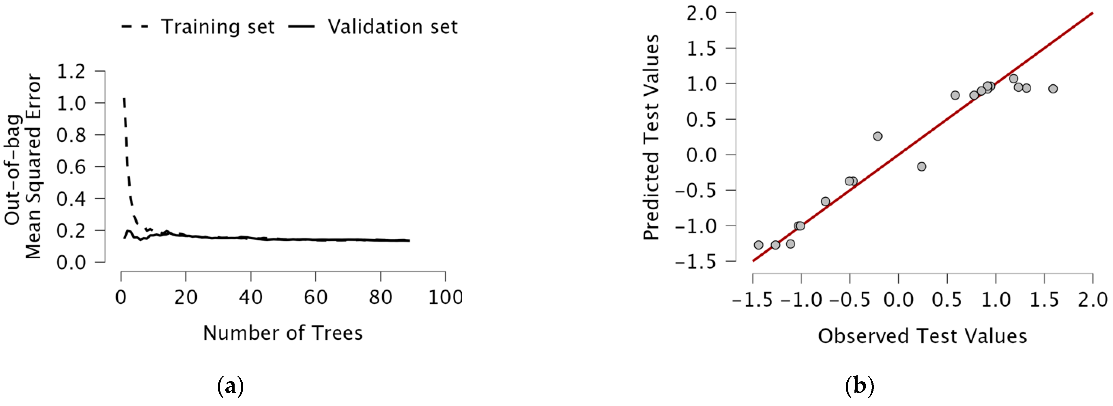
According to the results, shown in Figure 4a, 89 trees were tested and the OOB error was 0.132. Some literature suggest that a random forest should have a number of trees between 64–128 trees [47]. The RFR algorithm can predict the overall power output of the system very efficiently (R² = 0.942). Figure 4a shows the out-of-bag mean squared error plot as a function of the number of trees, where the dashed line represents the training set, and the continuous line represents the validation set. Meanwhile, Figure 4b represents the predictive performance plot of the random forest regression. It can be seen that the data points drop around the fitted curve. The greater the data points fit into the line, the more accurate the model is. The horizontal axes contain the observed test values, and the vertical coordinate is the predicted test values.

Furthermore, because of the low number of samples, the overfitting problem might not occur in case of the decision tree regression and the random forest regression. Nevertheless, the variable importance is similar for RFR and DTR. It can be concluded that intensity has the highest variable importance (total increase in node purity in case of intensity is 13.374), then the temperature difference (total increase in node purity in case of dT is 9.022), while the surface temperature of the DSSC has the lowest variable importance (total increase in node purity in case of temperature is 7.896).

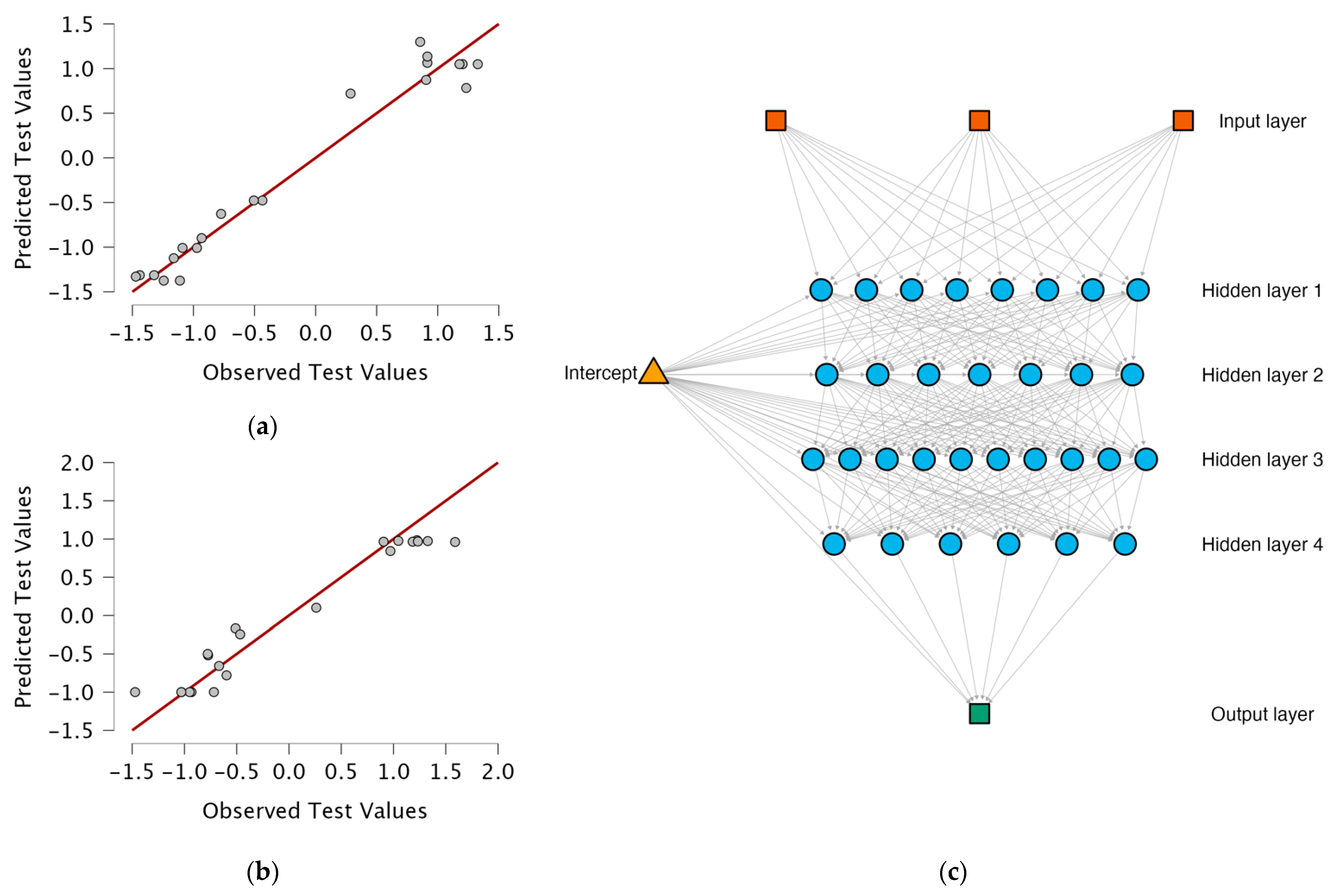
After the automatic splitting, the Manhattan distance function and fixed number of nearest neighbors were applied for K-nearest neighbors regression algorithm. The Manhattan distance function gave a better result for the KNN compared with the results of Euclidean distance function. According to the coefficient of determination of the KNN regression, the applied number of the nearest neighbors is regarded as appropriate (R² = 0.96). Figure 5a shows the predictive performance plot of the KNN regression, where the vertical coordinate is the prediction test values, and the horizontal coordinate is the observed test values. The last of the machine learning techniques which was used was the artificial neural network. Using ANN, two kinds of activation functions were taken into consideration: linear and hyperbolic tangent functions. The linear active function splits out the value, which was given, so it does not do anything to the weighted sum of the input. One of the disadvantages of the linear active function is that the last layer is a function of the first layer. In the interest of avoiding this phenomenon, a non-linear activation function (hyperbolic tangent activation function) was applied. Hyperbolic tangent activation function is similar to the sigmoid/logistic activation function, but because the hyperbolic tangent activation function is zero centered, and its gradients are not confined to move in a certain direction, hyperbolic tangent activation function is preferred to sigmoid activation function [48,49]. The network topology was optimized, with a population size of 20, the value of the generations at 10 and the parent selection as roulette wheel also known as fitness proportionate selection.

As a result of the hyperbolic activation function the number of hidden layers is four and the number of nodes is 31. Figure 5b shows the predictive performance plot of the tangent activation function used ANN. From the figure it can be seen that the values drop around the red fitted curve. Figure 5c shows the network structure plot of the ANN with three input layers and three hidden layers. The network weights are placed in tables. The input layers are the same as the previously used machine learning techniques. The maximum training repetitions were set to 500,000.

The performance of all algorithms was estimated based on the validation MSE, test MSE, RMSE, MAE, MAPE and R².

Table 5. Evaluation table of the applied machine learning algorithms with metrics.

ID	Machine Learning Algorithms	Metrics
		Validation MSE	Test MSE	RMSE	MAE	MAPE	R2
1	Decision tree regression	n/a	0.028	0.167	0.132	14.76%	0.972
2	Random forest regression	0.101	0.059	0.243	0.168	31.39%	0.942
3	K-nearest neighbors regression *	n/a	0.044	0.21	0.16	20.66%	0.96
4	Artificial neural network **	0.042	0.067	0.259	0.207	24.71%	0.95

MSE—mean squared error, RMSE—root mean square error, MAE—mean absolute error, MAPE—mean absolute percentage error, R²—coefficient of determination. * is in case of Manhattan distance function, ** is in case of hyperbolic tangent activation function.

shows the performance of the applied machine learning algorithms with the above-mentioned metrics. It is noticeable that all algorithms perform appropriately in terms of coefficient of determination (R²). If the value of R² is close to one, this indicates an exceptional result. In case of DTR and KNNR, there is no validation MSE because validation data selection was not available in the software. Taking Table 3 and Table 5 into account in connection with the resulted mean absolute percentage error values, it can be concluded that RFR, K-NNR, ANN algorithms fall into the reasonable precision. On the other hand, in case of MAPE, the Decision Tree Regression has the lowest value and fits into good precision. The difference between the validation MSE and test MSE is also an essential factor.

Comparing the mean squared error values of the ANN with the RFR, it can be seen that the absolute value between the validation MSE and test MSE is lower in case of the ANN (0.025) to the RFR (0.042). On the other hand, among the four regression algorithms, ANN algorithm shows high forecasting errors in test MSE = 0.067, RMSE = 0.259, MAE = 207.

The algorithm with minimum errors and with maximum R² indicates the most accurate method. According to Table 5 the decision tree regression has the highest coefficient of determination, and the other metrics are the lowest amongst the other methods. Hence, the performance of the decision tree regression algorithm can be observed to have the best performance when compared with the other algorithms. However, an overfitting problem can occur with a great deal of data in case of decision tree regression. In our model, considering the short data set, this might not occur.

4. Discussion

After comparing the four machine learning techniques, the performance of the built dye-sensitized solar cell–thermoelectric generator hybrid system was extrapolated based on the results of decision tree regression. In the previously presented experimental arrangement a pump was used to circulate water. During both the indoor and outdoor measurements, the energy scale was not calculated, but, according to the data, the energy scale is undisputedly negative. If the built system is extrapolated, a hydraulic pump is a mandatory piece of equipment to cool down the cold part of the thermoelectric generator. The main question is how many thermoelectric generators are needed for an inverter and how much area is required for that number of TEGs. For the extrapolation, the inverter presented in [50] was used. The unit specifications of the above-mentioned inverter are the following: the input voltage is 820 VDC, the output voltage is 440 VAC, and the output power is 30 kW. We made the following assumptions: all the DSSCs and TEGs used in the extrapolation are the same, which extends beyond the dimensions to the values from the experiment.

The TEGs are connected to the inverters in series. Nevertheless, to increase the power, TEGs can be connected in parallel. The extrapolation is made for the worst-case scenario, thus, the leaf node with the lowest performance (node-6) is taken into account on the basis of the results of the decision tree regression (see in Figure 3 and Table 4). Considering the average value of the voltage of the thermoelectric generator (U = 0.0135 V) belonging to node-6, 60,741 pieces of thermoelectric generators are needed, whose area is around 98 m². The calculation can be performed easily by dividing the desired inverter input voltage with the output voltage of one thermoelectric generator. Nonetheless, the required area is not far-fetched and does not deviate from reality because larger areas are used for solar farms. Taking an area of half a hectare (5000 m²) where the size of a solar panel is 2 m by 1 m, 3,125,000 pieces of thermoelectric generator can be installed on the back of DSSC panels. However, the total used area is 5000 m², with the area used by the solar panels at approximately 4000 m², due to the other items installed for the solar farm. As in the previous case, considering the worst-case-scenario, these 3,215,000 pieces of TEGs result in five inverters, where the TEG systems would be divided into five groups and connected to the main power line with the help of five inverters to ensure that the inverters operate under optimum voltage and power. Nonetheless, the overall DC power output was increased by 0.8% in the worst-case-scenario.

5. Conclusions

Recently, electricity generated from solar photovoltaics has been increasing significantly due to growing energy demand, and the huge concentration of carbon-dioxide in the atmosphere. DSSCs are considered to be promising, forward-looking solar cell devices, because of their low cost and easy production. If a DSSC is exposed to sunlight, thermal energy is accumulated inside the device, which has a reducing effect on the maximum power output. Utilizing this thermal energy via Seebeck effect can convert thermal energy into electric current. DSSC–TEG hybrid systems have been developed and presented in literature, in which the tests were taken in laboratory environments and not outdoor conditions. Moreover, the applied data evaluation methods belong to conventional analysis or simulation methods. This study proposed a performance analysis of a designed and built DSSC–TEG hybrid system using machine learning techniques. Laboratory measurements were planned and taken. Outside measurements were obtained based on the laboratory measurements, data processing was applied in order to transform the scale data type to ordinary data type. The analysis was performed to predict the maximum power output of the DSSC–TEG hybrid system, where the predictors are intensity, surface temperature of the DSSC, and temperature difference between the two sides of the TEG.

In this study, four machine learning techniques were analyzed: decision tree regression, random forest regression, K-nearest neighbors regression, and artificial neural network. The performance of all algorithms was estimated on the basis of the validation MSE, test MSE, RMSE, MAE, MAPE and R². The algorithm with minimum errors and with maximum R² indicates the most accurate method. The decision tree regression has the highest coefficient of determination, and the other metrics are the lowest amongst the other methods. Hence, the performance of the decision tree regression algorithm can be observed to have the best performance when compared with the other algorithms. The following conclusion can be conducted from the results of the DTR:

• If the intensity is equal to or lower than 800 W/m², we can predict from only the value of intensity how much the overall power output of the system might be.
• If the intensity is lower than 400 W/m², the mean of the overall power output 0.167 mW/cm² (node-6).
• If the intensity is greater than or equals to 400 W/m² and lower than or equals to 500 W/m², the mean value of the power outcome is 0.194 mW/cm² (node-7).
• If the value of intensity is greater than 500 W/m² and is equal to or lower than 800 W/m², the mean value of the power outcome is 0.224 W/cm² (node-8).
• If the intensity is higher than 800 W/m² and the temperature difference between the two sides of the TEG is lower than 8 °C, the predicted power outcome is 0.329 mW/cm² (node-9).
• If the intensity is higher than 800 W/m², and the temperature difference is equal to or greater than 8 °C and is equal to or lower than 12 °C, and the surface temperature of the DSSC is equal to or greater than 38 °C and equals to or lower than 42 °C, the predicted mean of the overall power output of the built DSSC–TEG hybrid system is 0.342 mW/cm² (node-10).
• If the intensity is higher than 800 W/m², and the temperature difference is equal to or greater than 8 °C and equals to or lower than 12 °C, and the surface temperature of the DSSC is greater than or equals to 8 °C and lower than 38 °C, the predicted power outcome value is 0.375 mW/cm² (node-11).

Consequently, the performance of the designed and built DSSC–TEG hybrid system was extrapolated based on the results of the DTR. Thus, in the worst-case scenario, the leaf node with the lowest performance (node-6) is taken into account on the basis of the results of the decision tree regression. The main question was how many thermoelectric generators are needed for an inverter to operate a hydraulic pump which circulates water, and how much area is required for the number of TEGs. Considering the average value of the voltage of the thermoelectric generator (U = 0.0135 V) belonging to node-6, 60,741 pieces of thermoelectric generators are needed whose area is around 98 m² for an inverter to operate a hydraulic pump to circulate water. As a result, in case of the worst-case scenario (node-6), the maximum power output of the DSSC–TEG hybrid system increased by 0.8%. Nevertheless, in the case of node-7, improvement can be detected in the performance, but it is lower (0.4%) than in the case of node-6. Moreover, in the case of node-8, the value of this improvement is 1%. Meanwhile, in the case of node-9, the performance of the DSSC–TEG was increased by 2.4% compared with the DSSC. Furthermore, in the case of node-10, the resulting increase in the performance was 3.2% compared to the performance of the DSSC. As a last result, in the case of node-11, the performance of the DSSC–TEG hybrid system was increased by 2.8% compared to the performance of the dye-sensitized solar cell.

References

- Devabhaktuni, V. Solar energy Trends and enabling technologies. Renew. Sustain. Energy Rev. 2013, 10, 555–564. [Google Scholar] [CrossRef]
- Li, X.; Liao, H.; Du, Y.-F.; Wang, C.; Wang, J.-W.; Liu, Y. Carbon dioxide emissions from the electricity sector in major countries: A decomposition analysis. Environ. Sci. Pollut. Res. 2018, 25, 6814–6825. [Google Scholar] [CrossRef] [PubMed]
- Omer, A.M. Energy, environment and sustainable development. Renew. Sustain. Energy Rev. 2008, 12, 2265–2300. [Google Scholar] [CrossRef]
- Schoden, F.; Dotter, M.; Knefelkamp, D.; Blachowicz, T.; Schwenzfeier Hellkamp, E. Review of State of the Art Recycling Methods in the Context of Dye Sensitized Solar Cells. Energies 2021, 14, 3741. [Google Scholar] [CrossRef]
- Malinowski, M.; Leon, J.I.; Abu-Rub, H. Solar Photovoltaic and Thermal Energy Systems: Current Technology and Future Trends. Proc. IEEE 2017, 105, 2132–2146. [Google Scholar] [CrossRef]
- O’Regan, B.; Grätzel, M. A low-cost, high-efficiency solar cell based on dye-sensitized colloidal TiO2 films. Nature 1991, 353, 737–740. [Google Scholar] [CrossRef]
- Wang, C.; Liu, M.; Rahman, S.; Pasanen, H.P.; Tian, J.; Li, J.; Deng, Z.; Zhang, H.; Vivo, P. Hydrogen bonding drives the self-assembling of carbazole-based hole-transport material for enhanced efficiency and stability of perovskite solar cells. Nano Energy 2022, 101, 107604. [Google Scholar] [CrossRef]
- Li, R.; Li, C.; Liu, M.; Vivo, P.; Zheng, M.; Dai, Z.; Zhan, J.; He, B.; Li, H.; Yang, W.; et al. Hydrogen-Bonded Dopant-Free Hole Transport Material Enables Efficient and Stable Inverted Perovskite Solar Cells. CCS Chem. 2022, 4, 3084–3094. [Google Scholar] [CrossRef]
- Gatto, E.; Lettieri, R.; Vesce, L.; Venanzi, M. Peptide Materials in Dye Sensitized Solar Cells. Energies 2022, 15, 5632. [Google Scholar] [CrossRef]
- Cornaro, C.; Renzi, L.; Pierro, M.; Di Carlo, A.; Guglielmotti, A. Thermal and Electrical Characterization of a Semi-Transparent Dye-Sensitized Photovoltaic Module under Real Operating Conditions. Energies 2018, 11, 155. [Google Scholar] [CrossRef] [Green Version]
- Gong, J.; Sumathy, K.; Qiao, Q.; Zhou, Z. Review on dye-sensitized solar cells (DSSCs): Advanced techniques and research trends. Renew. Sustain. Energy Rev. 2017, 68, 234–246. [Google Scholar] [CrossRef]
- Sharma, S.; Bulkesh, S.; Ghoshal, S.K.; Mohan, D. Dye sensitized solar cells: From genesis to recent drifts. Renew. Sustain. Energy Rev. 2017, 70, 529–537. [Google Scholar] [CrossRef]
- Kim, J.-H.; Han, S.-H. Energy Generation Performance of Window-Type Dye-Sensitized Solar Cells by Color and Transmittance. Sustainability 2020, 12, 8961. [Google Scholar] [CrossRef]
- Xu, L.; Xiong, Y.; Mei, A.; Hu, Y.; Rong, Y.; Zhou, Y.; Hu, B.; Han, H. Efficient Perovskite Photovoltaic-Thermoelectric Hybrid Device. Adv. Energy Mater. 2018, 8, 1702937. [Google Scholar] [CrossRef]
- Lepikko, S.; Miettunen, K.; Poskela, A.; Tiihonen, A.; Lund, P.D. Testing dye-sensitized solar cells in harsh northern outdoor conditions. Energy Sci. Eng. 2018, 6, 187–200. [Google Scholar] [CrossRef] [Green Version]
- Casano, G.; Piva, S. Experimental investigation of the performance of a thermoelectric generator based on Peltier cells. Exp. Therm. Fluid Sci. 2011, 35, 660–669. [Google Scholar] [CrossRef]
- Maneewan, S.; Chindaruksa, S. Thermoelectric Power Generation System Using Waste Heat from Biomass Drying. J. Elec. Mater. 2009, 38, 974–980. [Google Scholar] [CrossRef]
- Kossyvakis, D.N.; Voutsinas, G.D.; Hristoforou, E.V. Experimental analysis and performance evaluation of a tandem photovoltaic–Thermoelectric hybrid system. Energy Convers. Manag. 2016, 117, 490–500. [Google Scholar] [CrossRef]
- Guo, X.-Z.; Zhang, Y.-D.; Qin, D.; Luo, Y.-H.; Li, D.-M.; Pang, Y.-T.; Meng, Q.-B. Hybrid tandem solar cell for concurrently converting light and heat energy with utilization of full solar spectrum. J. Power Sources 2010, 195, 7684–7690. [Google Scholar] [CrossRef]
- Wang, N.; Han, L.; He, H.; Park, N.-H.; Koumoto, K. A novel high-performance photovoltaic–thermoelectric hybrid device. Energy Environ. Sci. 2011, 4, 3676. [Google Scholar] [CrossRef]
- Chang, H.; Kao, M.-J.; Huang, K.D.; Chen, S.-L.; Yu, Z.-R. A Novel Photo-Thermoelectric Generator Integrating Dye-sensitized Solar Cells with Thermoelectric Modules. Jpn. J. Appl. Phys. 2010, 49, 06GG08. [Google Scholar] [CrossRef]
- Chang, H.; Yu, Z.-R. Integration of Dye-Sensitized Solar Cells, Thermoelectric Modules and Electrical Storage Loop System to Constitute a Novel Photothermoelectric Generator. J. Nanosci. Nanotechnol. 2012, 12, 6811–6816. [Google Scholar] [CrossRef] [PubMed]
- Su, S.; Liu, T.; Wang, Y.; Chen, X.; Wang, J.; Chen, J. Performance optimization analyses and parametric design criteria of a dye-sensitized solar cell thermoelectric hybrid device. Appl. Energy 2014, 120, 16–22. [Google Scholar] [CrossRef]
- Kim, Y.J.; Choi, H.; Kim, C.S.; Lee, G.; Park, J.; Park, S.E.; Cho, B.J. Dye-Sensitized Solar Cell–Thermoelectric Hybrid Generator Utilizing Bipolar Conduction in a Unified Element. ACS Appl. Energy Mater. 2020, 3, 4155–4161. [Google Scholar] [CrossRef]
- Chang, H.; Kao, M.-J.; Cho, K.-C.; Chen, S.-L.; Chu, K.-H.; Chen, C.-C. Integration of CuO thin films and dye-sensitized solar cells for thermoelectric generators. Curr. Appl. Phys. 2011, 11, S19–S22. [Google Scholar] [CrossRef]
- Lee, D.; Jeong, J.-W.; Choi, G. Short Term Prediction of PV Power Output Generation Using Hierarchical Probabilistic Model. Energies 2021, 14, 2822. [Google Scholar] [CrossRef]
- Sutar, S.S.; Patil, S.M.; Kadam, S.J.; Kamat, R.K.; Kim, D.; Dongale, T.D. Analysis and Prediction of Hydrothermally Synthesized ZnO-Based Dye-Sensitized Solar Cell Properties Using Statistical and Machine-Learning Techniques. ACS Omega 2021, 6, 29982–29992. [Google Scholar] [CrossRef]
- Venkatraman, V.; Yemene, A.E.; de Mello, J. Prediction of Absorption Spectrum Shifts in Dyes Adsorbed on Titania. Sci. Rep. 2019, 9, 16983. [Google Scholar] [CrossRef] [Green Version]
- Maddah, H.A. Machine learning analysis on performance of naturally-sensitized solar cells. Opt. Mater. 2022, 128, 112343. [Google Scholar] [CrossRef]
- Li, F.; Peng, X.; Wang, Z.; Zhou, Y.; Wu, Y.; Jiang, M.; Xu, M. Machine Learning (ML)-Assisted Design and Fabrication for Solar Cells. Energy Environ. Mater. 2019, 2, 280–291. [Google Scholar] [CrossRef] [Green Version]
- Majidpour, M.; Nazaripouya, H.; Chu, P.; Pota, H.; Gadh, R. Fast Univariate Time Series Prediction of Solar Power for Real-Time Control of Energy Storage System. Forecasting 2018, 1, 107–120. [Google Scholar] [CrossRef] [Green Version]
- Krechowicz, M.; Krechowicz, A.; Lichołai, L.; Pawelec, A.; Piotrowski, J.Z.; Stępień, A. Reduction of the Risk of Inaccurate Prediction of Electricity Generation from PV Farms Using Machine Learning. Energies 2022, 15, 4006. [Google Scholar] [CrossRef]
- Wei, C.-C. Predictions of Surface Solar Radiation on Tilted Solar Panels using Machine Learning Models: A Case Study of Tainan City, Taiwan. Energies 2017, 10, 1660. [Google Scholar] [CrossRef] [Green Version]
- Hosseinnezhad, M.; Saeb, M.R.; Garshasbi, S.; Mohammadi, Y. Realization of manufacturing dye-sensitized solar cells with possible maximum power conversion efficiency and durability. Sol. Energy 2017, 149, 314–322. [Google Scholar] [CrossRef]
- Varga, Z.; Racz, E. Experimental Investigation of the Performance of a Thermoelectric Generator. In Proceedings of the 2022 IEEE 20th Jubilee World Symposium on Applied Machine Intelligence and Informatics (SAMI), Poprad, Slovakia, 2 March 2022; pp. 159–164. [Google Scholar]
- Bodnár, I.; Koós, D.; Iski, P.; Skribanek, Á. Design and Construction of a Sun Simulator for Laboratory Testing of Solar Cells. Acta Polytech. Hung. 2020, 17, 165–184. [Google Scholar] [CrossRef]
- Charbuty, B.; Abdulazeez, A. Classification Based on Decision Tree Algorithm for Machine Learning. JASTT 2021, 2, 20–28. [Google Scholar] [CrossRef]
- Khandakar, A.; Chowdhury, E.H.M.; Khoda, M.-K.; Benhmed, K.; Touati, F.; Al-Hitmi, M.; Gonzales, S.P.A., Jr. Machine Learning Based Photovoltaics (PV) Power Prediction Using Different Environmental Parameters of Qatar. Energies 2019, 12, 2782. [Google Scholar] [CrossRef] [Green Version]
- Ordoñez Palacios, L.E.; Bucheli Guerrero, V.; Ordoñez, H. Machine Learning for Solar Resource Assessment Using Satellite Images. Energies 2022, 15, 3985. [Google Scholar] [CrossRef]
- Singh, U.; Rizwan, M.; Alaraj, M.; Alsaidan, I. A Machine Learning-Based Gradient Boosting Regression Approach for Wind Power Production Forecasting: A Step towards Smart Grid Environments. Energies 2021, 14, 5196. [Google Scholar] [CrossRef]
- Alghamdi, H.A. A Time Series Forecasting of Global Horizontal Irradiance on Geographical Data of Najran Saudi Arabia. Energies 2022, 15, 928. [Google Scholar] [CrossRef]
- Wang, F.; Zhen, Z.; Wang, B.; Mi, Z. Comparative Study on KNN and SVM Based Weather Classification Models for Day Ahead Short Term Solar PV Power Forecasting. Appl. Sci. 2017, 8, 28. [Google Scholar] [CrossRef] [Green Version]
- Bakay, M.S.; Ağbulut, Ü. Electricity production based forecasting of greenhouse gas emissions in Turkey with deep learning, support vector machine and artificial neural network algorithms. J. Clean. Prod. 2021, 285, 125324. [Google Scholar] [CrossRef]
- Michalak, P. Thermal—Airflow Coupling in Hourly Energy Simulation of a Building with Natural Stack Ventilation. Energies 2022, 15, 4175. [Google Scholar] [CrossRef]
- Racz, E.; Varga, Z. Investigation of the Maximum Power Point on a DSSC Solar Cell based on the Incoming Light Irradiation and Temperature. In Proceedings of the 2020 IEEE 3rd International Conference and Workshop in Óbuda on Electrical and Power Engineering (CANDO-EPE), Budapest, Hungary, 18 November 2020; pp. 161–166. [Google Scholar]
- Varga, Z.; Racz, E. Influence of the Cell Temperature on the Performance of a Dye Sensitized Solar Cell. In Proceedings of the 2021 IEEE 19th World Symposium on Applied Machine Intelligence and Informatics (SAMI), Herl’any, Slovakia, 21 January 2021; pp. 175–180. [Google Scholar]
- Oshiro, T.M.; Perez, P.S.; Baranauskas, J.A. How Many Trees in a Random Forest? In Proceedings of the International Workshop on Machine Learning and Data Mining in Pattern Recognition Berlin, Germany, 13–20 July 2012; 15p.
- Kiliçarslan, S.; Adem, K.; ÇeliK, M. An overview of the activation functions used in deep learning algorithms. J. New Results Sci. 2021, 10, 75–88. [Google Scholar] [CrossRef]
- Khan, J.A.; Irfan, M.; Irawan, S.; Yao, F.K.; Abdul Rahaman, M.S.; Shahari, A.R.; Glowacz, A.; Zeb, N. Comparison of Machine Learning Classifiers for Accurate Prediction of Real-Time Stuck Pipe Incidents. Energies 2020, 13, 3683. [Google Scholar] [CrossRef]
- Uyanık, T.; Ejder, E.; Arslanoğlu, Y.; Yalman, Y.; Terriche, Y.; Su, C.-L.; Guerrero, J.M. Thermoelectric Generators as an Alternative Energy Source in Shipboard Microgrids. Energies 2022, 15, 4248. [Google Scholar] [CrossRef]
Figure 1.
(a) A 3D drawing of the structure of the sandwich-like target system in a water bath where the blue cylinder is the water pipe in which water flows to cool down the cold side of the thermoelectric generator resulting in a temperature difference between the two sides of the thermoelectric generator. The numbers in the circle represent the parts of the target system: number 1: extruded polystyrene, number 2: the dye-sensitized solar cell, number 3: the black part is the aluminum sheet, the orange part is thermal grease, and the white part is the thermoelectric generator, number 4: heat sink, number 5: water bath, and number 6: water pipes. (b) The built sun simulator device with the built DSSC–TEG hybrid system in a water bath where water flows. The target system is located under a lamp array. The incoming irradiation intensity was 100 mW/cm2. The number 1 represents the LED lamp, the number 2 is the halogen lamps, and the number 3 represents the target system.
Figure 2.
(a) Schematic overview of the target system where the hydraulic pump (shown as number 7) is inside the receiving tank (shown as number 8). The hydraulic pump circulated the water in the water bath (shown as number 5). The numbers in the circle represent the parts of the target system: number 1: extruded polystyrene, number 2: the dye-sensitized solar cell, number 3: the black part is the aluminum sheet, the orange part is thermal grease, and the white part is the thermoelectric generator, number 4: heat sink, number 5: water bath, and number 6: water pipes. (b) The built and tested DSSC–TEG hybrid system during the outside experiment with the cables, which were used to measure the target parameter and the predictor parameters. The measurements were time dependent.
Figure 3.
Decision tree model to identify the possible outcomes of the overall power output of the DSSC–TEG hybrid system.
Figure 4.
Results of prediction of the random forest regression: (a) out-of-bag mean squared error plot in function of the number of trees, where the dashed line is in case of the training set and the continuous line is in case of the validation set. (b) Predictive performance plot, where the vertical coordinate is the predicted test values, and the horizontal coordinate is the observed test values.
Figure 5.
(a) Predictive performance plot in case of the K-nearest neighbors regression method. (b) Predictive performance plot in case of the artificial neural network method using hyperbolic tangent activation function. (c) Network structure plot of the ANN with three input layers and three hidden layers. The number of nodes is 31.