
Double-Slope Solar Still Productivity Based on the Number of Rubber Scraper Motions
 , , ,
, , ,  and
and 
Abstract
:1. Introduction
1.1. Research Background
1.2. Adopted Literature
1.3. Research Significant and Motivation
1.4. Research Problem Statement and Objectives
2. Methodology
2.1. Heat and Mass Transfer Mechanisms in Solar Still
2.1.1. Convective Heat Transfer from Water to Condensing Glass Cover
2.1.2. Evaporative Heat Transfer from Salty Water toward the Condensing Cover
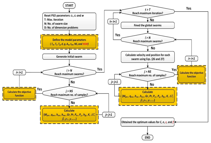
2.2. Developed PSO–HYSS Model
2.3. Hourly Yield Model for the DSSSHS Created Employing PSO
2.3.1. Objective Functions
2.3.2. Particle Swarm Optimization (PSO) Algorithm
2.3.3. Convergence Criteria
2.4. Implementing PSO with HYSS Model
- After a random position is specified for each particle in the space, the swarm is initialized.
- In the developed PSO–HYSS model, the objective function of each particle is evaluated.
- For each particle, the objective function’s value is then matched with the value of its . The current value is set as if the former is better than the current value. Meanwhile, represents the current position of the particle .
- The particle whose objective function has the best value is named as , and its position is presented by .
- Equations (26) and (27) are used to modify particles’ positions and velocities.
- The steps from 2 to 5 are repeated till reaching the maximum number of iterations or achieving a satisfying value of the objective function.
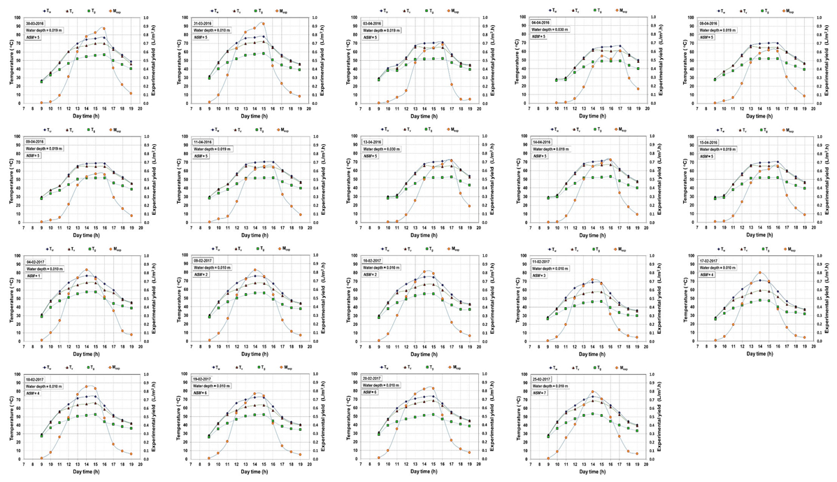
3. Experimental Database
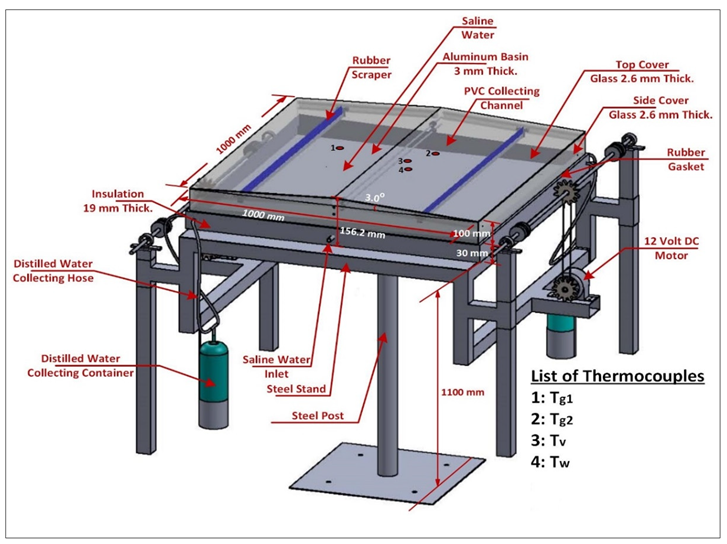
3.1. Setup of the Experiment
3.2. Experimental Results
4. Results and Discussion
4.1. Analysis of Developed PSO–HYSS Model
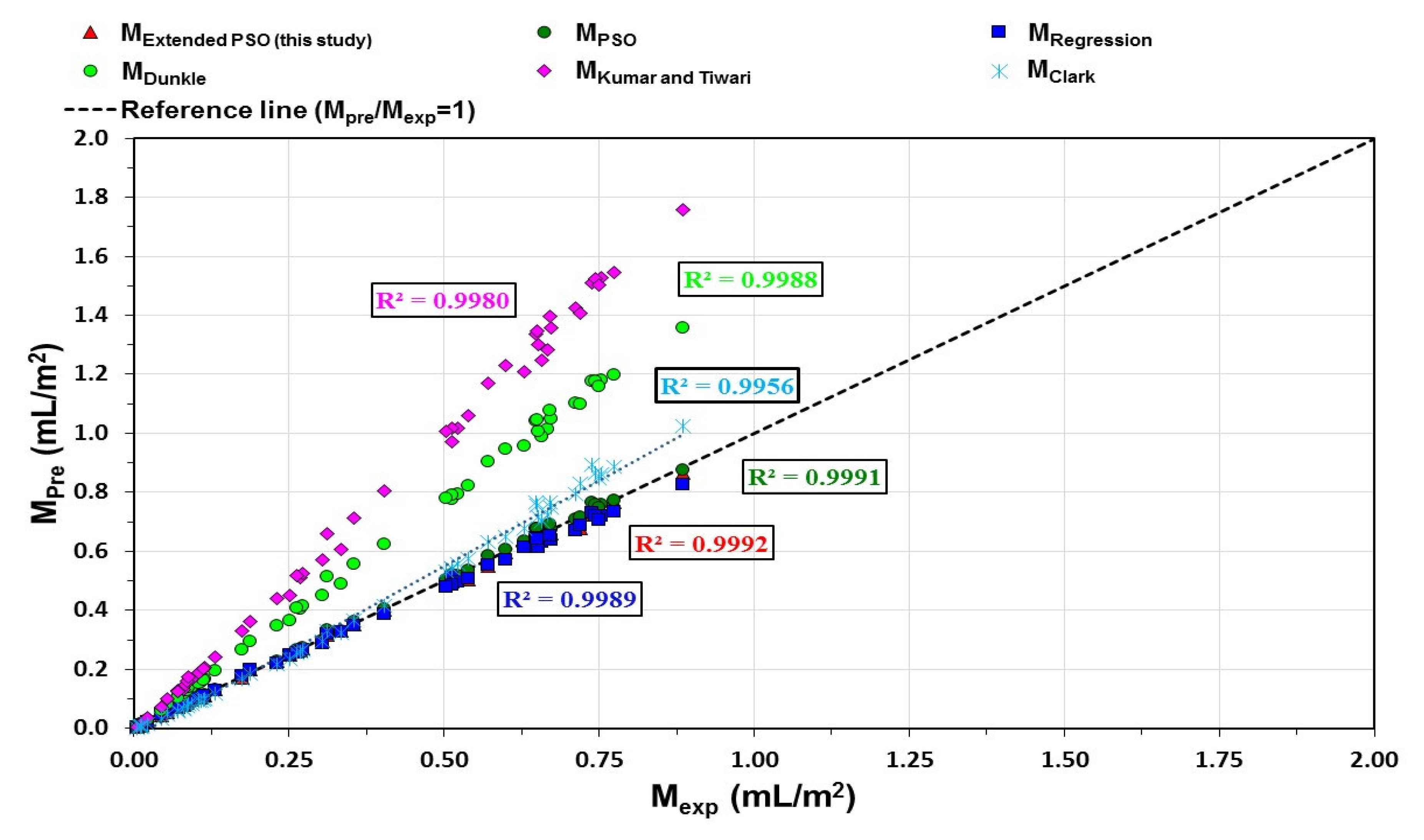
4.2. Verification of Developed PSO–HYSS Model
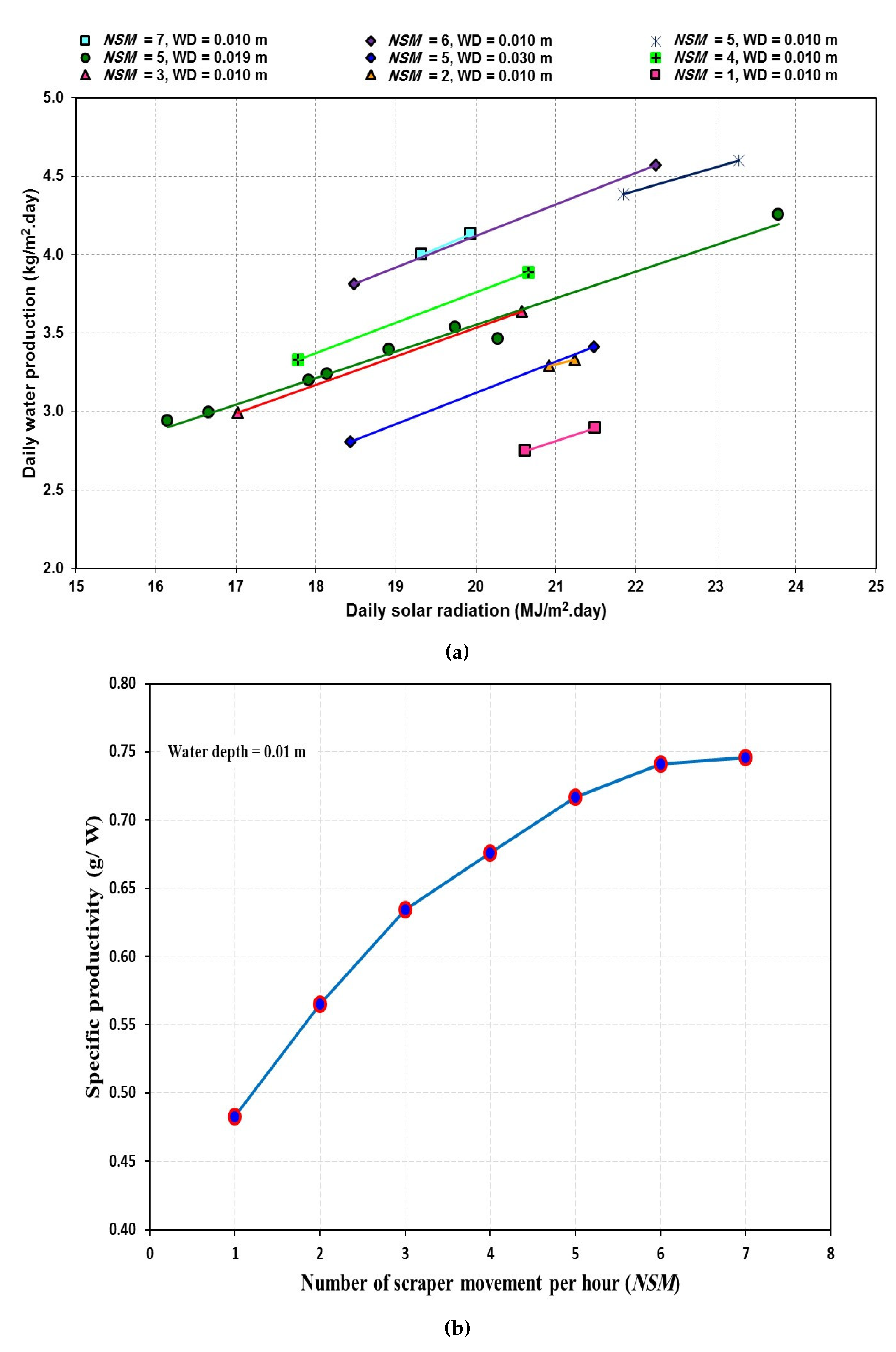
4.3. Effects of Solar Radiation and NSM on the Productivity of Solar Still
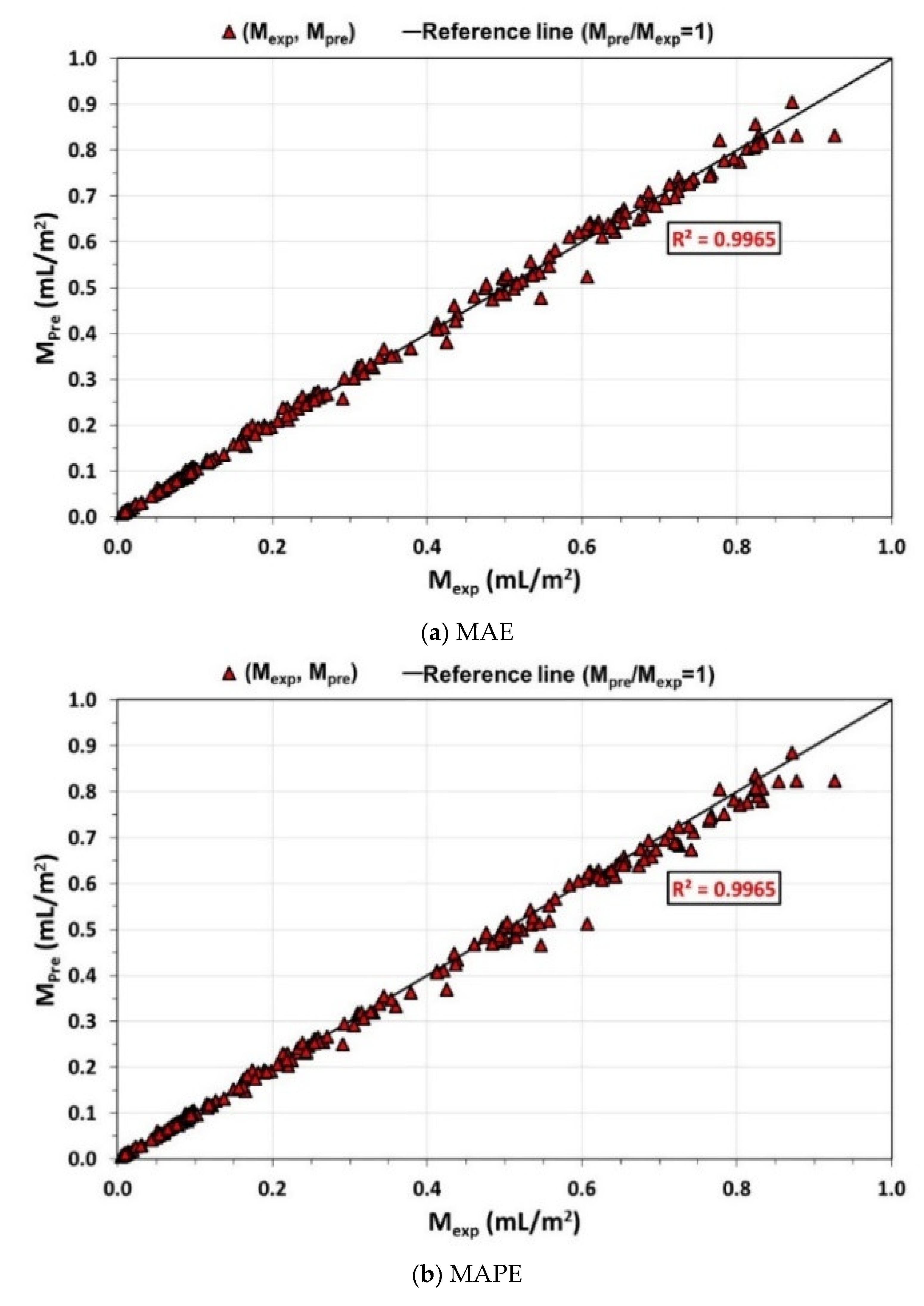
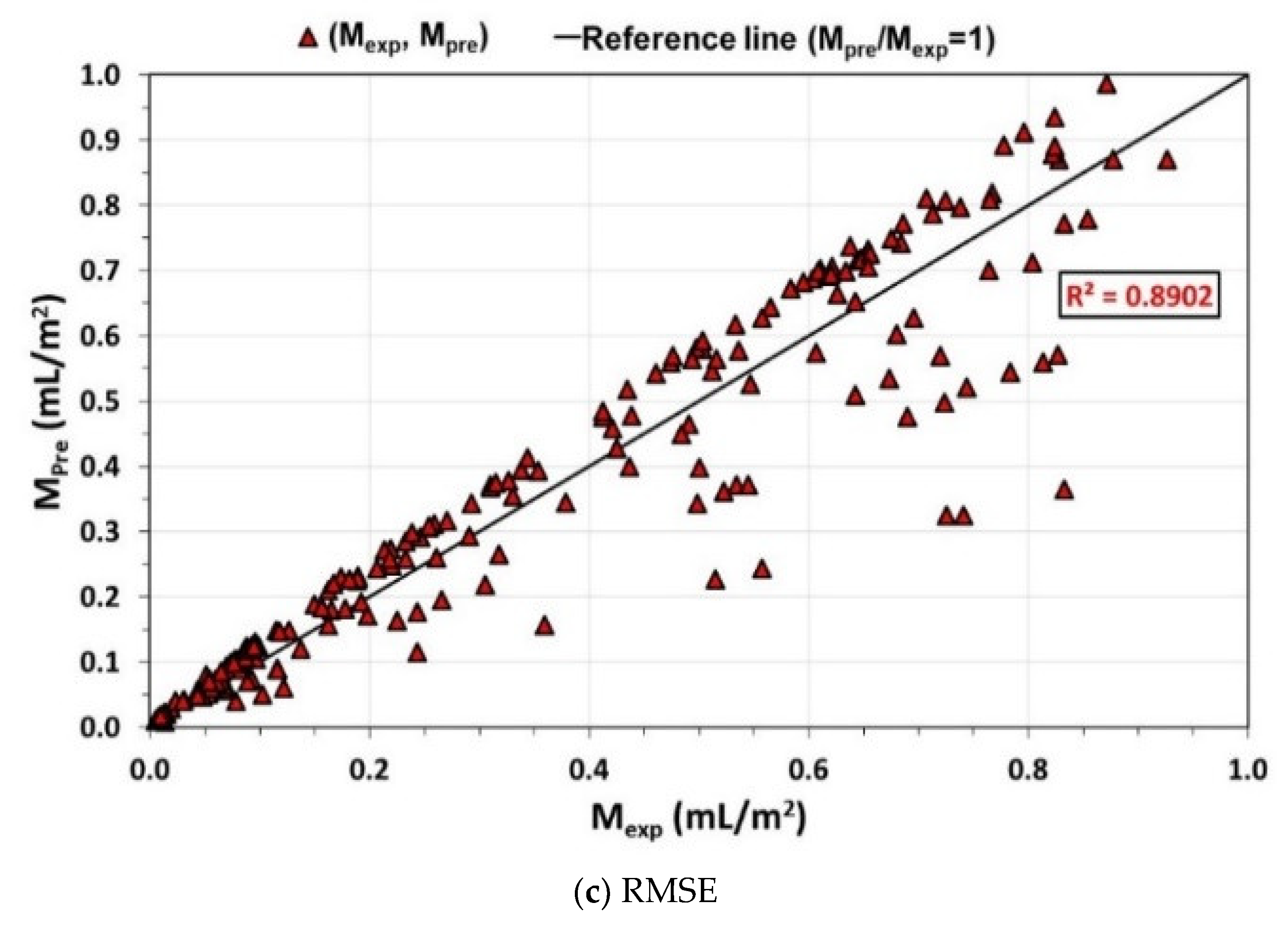
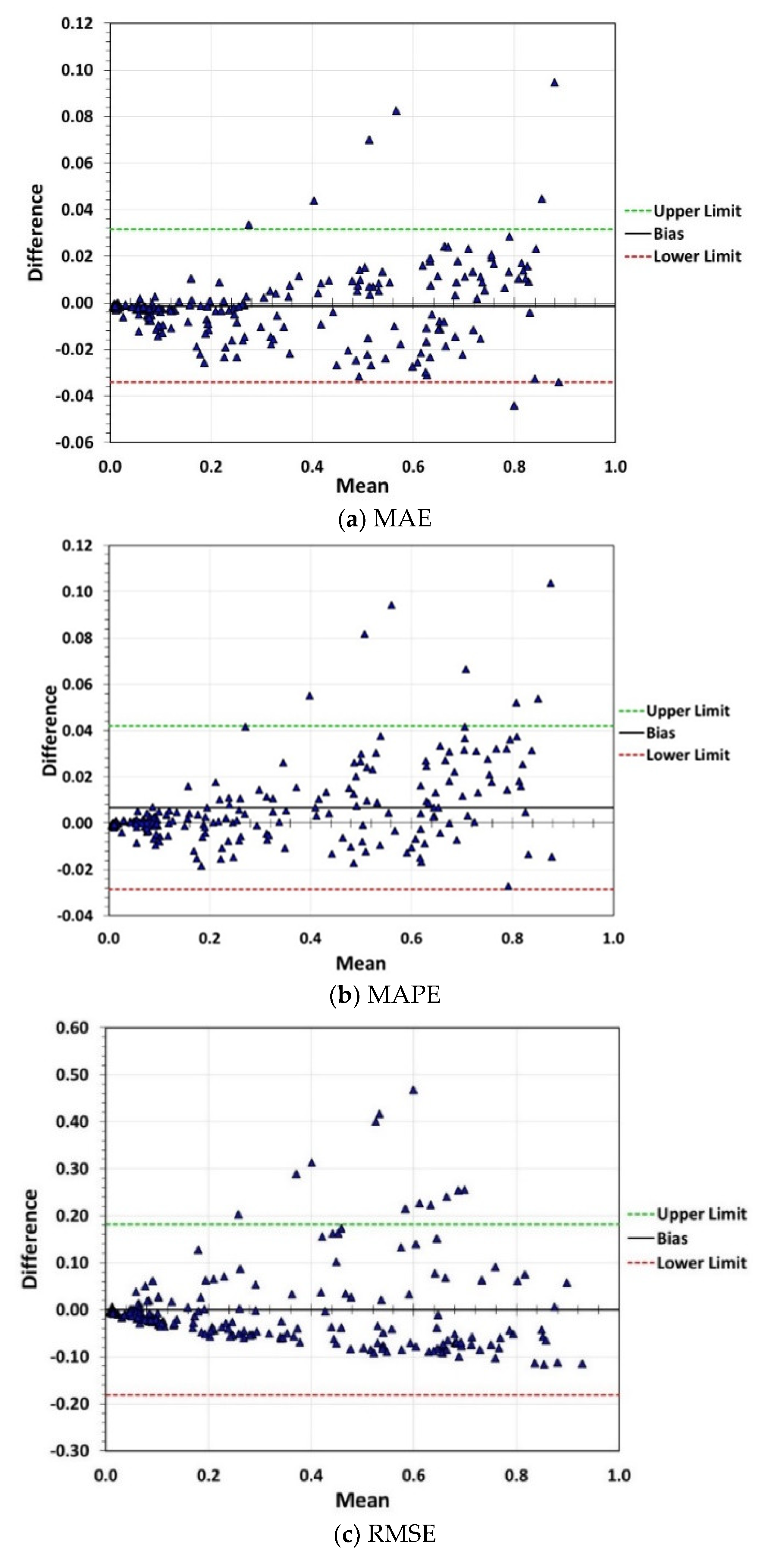
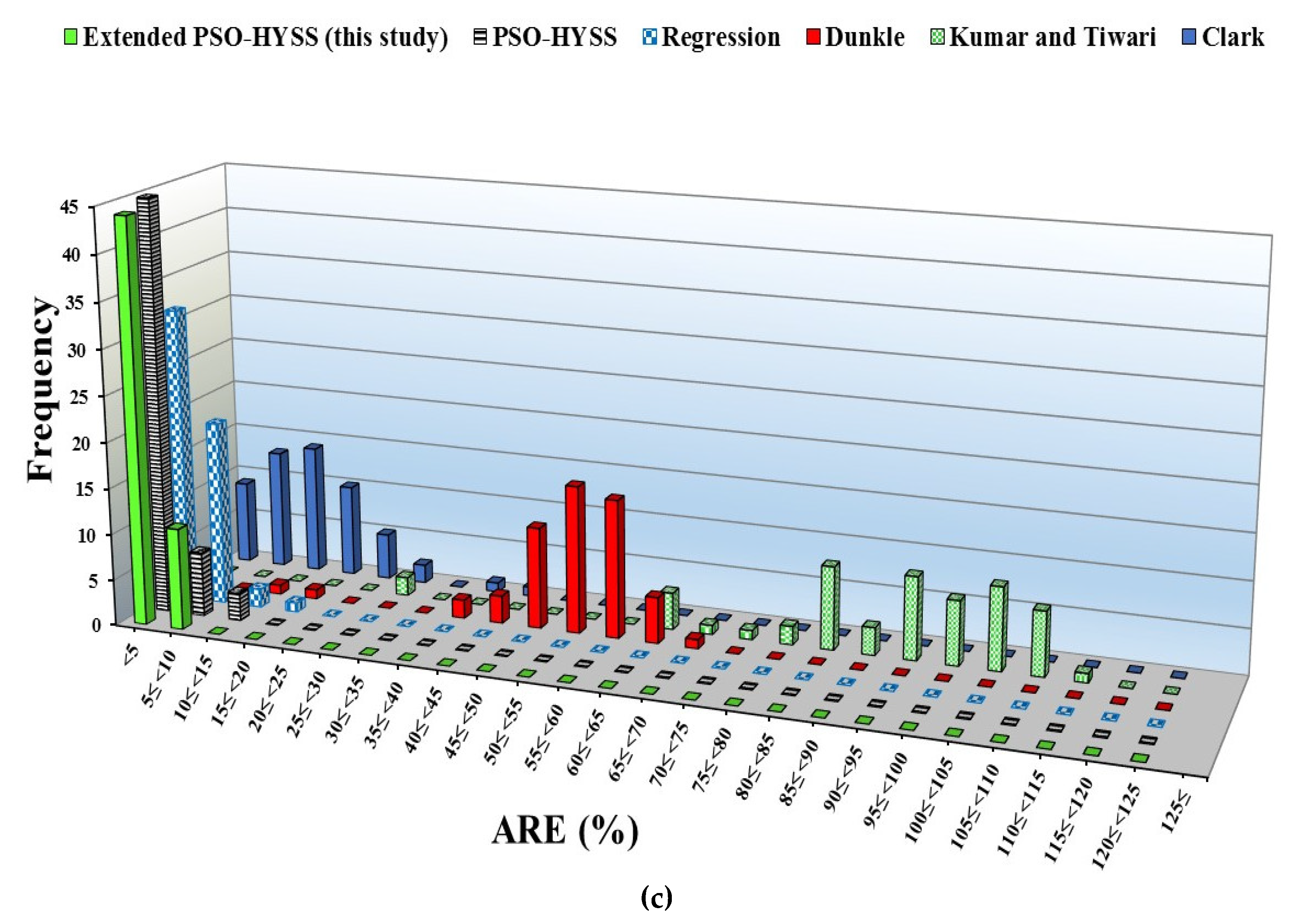
4.4. Error Analysis
4.5. Uncertainty Analysis
4.6. Discussion
5. Conclusions
- ▘
- NSM revealed a significant effect on DSSSHS productivity and HYSS prediction accuracy.
- ▘
- The specific productivity of the DSSSHS with a fixed water depth of 0.01 m is directly proportional to the magnitude of NSM, in which the specific productivity increases with NSM. To inspect the impacts of NSM on the predicted yield accuracy of DSSSHS, an improved PSO–HYSS was developed with consideration of the effects of NSM. Comparing the predicted and measured value results indicated that the PSO–HYSS model gave the superior predictability performance yields with the other models. Thus, the proposed model was confirmed to be effective and efficient for the prediction process.
- ▘
- By validating the results of the error analysis, PSO-HYSS attained the lower frequency “ARE ≥ 10%” and high frequency at low “ARE < 5%”. Models within the spectrum of acceptable error distribution may be ordered as follows: developed PSO–HYSS, regression, and Clark’s. Thus, in terms of error prediction, the developed PSO–HYSS model can be considered the best among other models.
- ▘
- Statistical analysis indicated a consistent results for the developed PSO-HYSS model.
Author Contributions
Funding
Data Availability Statement
Acknowledgments
Conflicts of Interest
Appendix A. Flowchart of Developed PSO–HYSS Model for HYSS Estimation

Appendix B. Isometric Diagram of DSSSHS

Appendix C. Experimental Records of 207 Datasets (19 days) for Developed PSO–HYSS Model Construction. Note: NSM Is the Number of Scraper Motions per Hour

Appendix D. Experimental Records of Fifty-Five Datasets for the Developed PSO–HYSS Model Verification

Appendix E. Convergence of Different Swarm Sizes Used in Developed PSO–HYSS Model

References
- Khawaji, A.D.; Kutubkhanah, I.K.; Wie, J.-M. Advances in seawater desalination technologies. Desalination 2008, 221, 47–69. [Google Scholar] [CrossRef]
- Kabeel, A.E. Performance of solar still with a concave wick evaporation surface. Energy 2009, 34, 1504–1509. [Google Scholar] [CrossRef]
- Dev, R.; Tiwari, G.N. Characteristic equation of the inverted absorber solar still. Desalination 2011, 269, 67–77. [Google Scholar] [CrossRef]
- Abu-Arabi, M.; Zurigat, Y.; Al-Hinai, H.; Al-Hiddabi, S. Modeling and performance analysis of a solar desalination unit with double-glass cover cooling. Desalination 2002, 143, 173–182. [Google Scholar] [CrossRef]
- Arunkumar, T.; Jayaprakash, R.; Ahsan, A.; Denkenberger, D.; Okundamiya, M.S. Effect of water and air flow on concentric tubular solar water desalting system. Appl. Energy 2013, 103, 109–115. [Google Scholar] [CrossRef]
- Kabeel, A.E.; Khairat Dawood, M.M.; Ramzy, K.; Nabil, T.; Elnaghi, B.; Elkassar, A. Enhancement of single solar still integrated with solar dishes: An experimental approach. Energy Convers. Manag. 2019, 196, 165–174. [Google Scholar] [CrossRef]
- Abu-Hijleh, B.A.; Rababa’h, H.M. Experimental study of a solar still with sponge cubes in basin. Energy Convers. Manag. 2003, 44, 1411–1418. [Google Scholar] [CrossRef]
- Alawee, W.H.; Dhahad, H.A.; Ahmed, I.S.; Mohammad, T.A. Experimental investigation on an elevated basin solar still with integrated internal reflectors and inclined fins. J. Eng. Sci. Technol. 2021, 16, 762–777. [Google Scholar]
- Taqi, R.N.; Abdul Redha, Z.A.; Mustafa, F.I. Experimental Investigation of a Single Basin-Single Slope Solar Still Coupled with Evacuated Tube Solar Collector. J. Eng. 2021, 27, 16–34. [Google Scholar] [CrossRef]
- Tabrizi, F.F.; Sharak, A.Z. Experimental study of an integrated basin solar still with a sandy heat reservoir. Desalination 2010, 253, 195–199. [Google Scholar] [CrossRef]
- Al_qasaab, M.R.; Abed, Q.A.; Abd Al-wahid, W.A. Enhancement the Solar Distiller Water By Using Parabolic Dish Collector With Single Slope Solar Still. J. Therm. Eng. 2021, 7, 1000–1015. [Google Scholar] [CrossRef]
- Ahsan, A.; Fukuhara, T. Condensation Mass Transfer in Unsaturated Humid Air Inside Tubular Solar Still. J. Hydrosci. Hydraul. Eng. 2010, 28, 31–42. [Google Scholar]
- Danish, S.N.; El-Leathy, A.; Alata, M.; Al-Ansary, H. Enhancing solar still performance using vacuum pump and geothermal energy. Energies 2019, 12, 539. [Google Scholar] [CrossRef] [Green Version]
- Dumka, P.; Sharma, A.; Kushwah, Y.; Raghav, A.S.; Mishra, D.R. Performance evaluation of single slope solar still augmented with sand-filled cotton bags. J. Energy Storage 2019, 25, 100888. [Google Scholar] [CrossRef]
- Abdel-Rehim, Z.S.; Lasheen, A. Experimental and theoretical study of a solar desalination system located in Cairo, Egypt. Desalination 2007, 217, 52–64. [Google Scholar] [CrossRef]
- Attia, M.E.H.; Driss, Z.; Manokar, A.M.; Sathyamurthy, R. Effect of aluminum balls on the productivity of solar distillate. J. Energy Storage 2020, 30, 101466. [Google Scholar] [CrossRef]
- Esfahani, J.A.; Rahbar, N.; Lavvaf, M. Utilization of thermoelectric cooling in a portable active solar still—An experimental study on winter days. Desalination 2011, 269, 198–205. [Google Scholar] [CrossRef]
- Guo, H.; Tao, H.; Salih, S.Q.; Yaseen, Z.M. Optimized parameter estimation of a PEMFC model based on improved Grass Fibrous Root Optimization Algorithm. Energy Rep. 2020, 6, 1510–1519. [Google Scholar] [CrossRef]
- Ahsan, A.; Syuhada, N.; Jolhi, E.; Darain, K.M.; Rowshon, M.K.; Jakariya, M.; Shafie, S.; Ghazali, A.H. Assessment of distillate water quality parameters produced by solar still for potable usage. Fresenius Environ. Bull. 2014, 23, 859–866. [Google Scholar]
- Sathyamurthy, R.; Nagarajan, P.K.; Subramani, J.; Vijayakumar, D.; Mohammed Ashraf Ali, K. Effect of Water Mass on Triangular Pyramid Solar Still Using Phase Change Material as Storage Medium. Energy Procedia 2014, 61, 2224–2228. [Google Scholar] [CrossRef] [Green Version]
- Velmurugan, V.; Gopalakrishnan, M.; Raghu, R.; Srithar, K. Single basin solar still with fin for enhancing productivity. Energy Convers. Manag. 2008, 49, 2602–2608. [Google Scholar] [CrossRef]
- Arunkumar, T.; Velraj, R.; Ahsan, A.; Khalifa, A.J.N.; Shams, S.; Denkenberger, D.; Sathyamurthy, R. Effect of parabolic solar energy collectors for water distillation. Desalin. Water Treat. 2015, 57, 21234–21242. [Google Scholar] [CrossRef]
- Arunkumar, T.; Velraj, R.; Denkenberger, D.C.; Sathyamurthy, R.; Kumar, K.V.; Ahsan, A. Productivity enhancements of compound parabolic concentrator tubular solar stills. Renew. Energy 2016, 88, 391–400. [Google Scholar] [CrossRef]
- Karimi Estahbanati, M.R.; Ahsan, A.; Feilizadeh, M.; Jafarpur, K.; Ashrafmansouri, S.-S.; Feilizadeh, M. Theoretical and experimental investigation on internal reflectors in a single-slope solar still. Appl. Energy 2016, 165, 537–547. [Google Scholar] [CrossRef]
- Ahsan, A.; Islam, K.M.S.; Fukuhara, T.; Ghazali, A.H. Experimental study on evaporation, condensation and production of a new Tubular Solar Still. Desalination 2010, 260, 172–179. [Google Scholar] [CrossRef]
- Rahbar, N.; Esfahani, J.A.; Asadi, A. An experimental investigation on productivity and performance of a new improved design portable asymmetrical solar still utilizing thermoelectric modules. Energy Convers. Manag. 2016, 118, 55–62. [Google Scholar] [CrossRef]
- Arunkumar, T.; Jayaprakash, R.; Denkenberger, D.; Ahsan, A.; Okundamiya, M.S.; Kumar, S.; Tanaka, H.; Aybar, H.Ş. An experimental study on a hemispherical solar still. Desalination 2012, 286, 342–348. [Google Scholar] [CrossRef]
- Ali, H.M. Experimental study on air motion effect inside the solar still on still performance. Energy Convers. Manag. 1991, 32, 67–70. [Google Scholar] [CrossRef]
- Rashidi, S.; Bovand, M.; Esfahani, J.A. Optimization of partitioning inside a single slope solar still for performance improvement. Desalination 2016, 395, 79–91. [Google Scholar] [CrossRef]
- Kabeel, A.E.; Omara, Z.M.; Essa, F.A. Improving the performance of solar still by using nanofluids and providing vacuum. Energy Convers. Manag. 2014, 86, 268–274. [Google Scholar] [CrossRef]
- Alawee, W.H. Improving the productivity of single effect double slope solar still by modification simple. J. Eng. 2015, 21, 50–60. [Google Scholar]
- Patel, S.K.; Singh, D.; Devnani, G.L.; Sinha, S.; Singh, D. Potable water production via desalination technique using solar still integrated with partial cooling coil condenser. Sustain. Energy Technol. Assess. 2021, 43, 100927. [Google Scholar] [CrossRef]
- Mevada, D.; Panchal, H.; Ahmadein, M.; Zayed, M.E.; Alsaleh, N.A.; Djuansjah, J.; Moustafa, E.B.; Elsheikh, A.H.; Sadasivuni, K.K. Investigation and performance analysis of solar still with energy storage materials: An energy-exergy efficiency analysis. Case Stud. Therm. Eng. 2022, 29, 101687. [Google Scholar] [CrossRef]
- Thalib, M.M.; Manokar, A.M.; Essa, F.A.; Vasimalai, N.; Sathyamurthy, R.; Garcia Marquez, F.P. Comparative Study of Tubular Solar Stills with Phase Change Material and Nano-Enhanced Phase Change Material. Energies 2020, 13, 3989. [Google Scholar] [CrossRef]
- Rashidi, S.; Akar, S.; Bovand, M.; Ellahi, R. Volume of fluid model to simulate the nanofluid flow and entropy generation in a single slope solar still. Renew. Energy 2018, 115, 400–410. [Google Scholar]
- Khalifa, A.J.N. On the effect of cover tilt angle of the simple solar still on its productivity in different seasons and latitudes. Energy Convers. Manag. 2011, 52, 431–436. [Google Scholar] [CrossRef]
- Abdallah, S.; Badran, O.; Abu-Khader, M.M. Performance evaluation of a modified design of a single slope solar still. Desalination 2008, 219, 222–230. [Google Scholar]
- Aybar, H.Ş.; Egelioğlu, F.; Atikol, U. An experimental study on an inclined solar water distillation system. Desalination 2005, 180, 285–289. [Google Scholar]
- Al-Sulttani, A.O.; Ahsan, A.; Rahman, A.; Nik Daud, N.N.; Idrus, S. Heat transfer coefficients and yield analysis of a double-slope solar still hybrid with rubber scrapers: An experimental and theoretical study. Desalination 2017, 407, 61–74. [Google Scholar] [CrossRef]
- Dunkle, R.V. Solar water distillation: The roof type still and a multiple effect diffusion still. In Proceedings of the International Heat Transfer Conference, University of Colorado, Boulder, CO, USA, 28 August–1 September 1961; Volume 5, p. 895. [Google Scholar]
- Tsilingiris, P.T. Analysis of the heat and mass transfer processes in solar stills—The validation of a model. Sol. Energy 2009, 83, 420–431. [Google Scholar]
- de Paula, A.C.O.; Ismail, K.A.R. Comprehensive investigation of water film thickness effects on the heat and mass transfer of an inclined solar still. Desalination 2021, 500, 114895. [Google Scholar] [CrossRef]
- Singh, R.G.; Tiwari, G.N. Simulation performance of single slope solar still by using iteration method for convective heat transfer coefficient. Groundw. Sustain. Dev. 2020, 10, 100287. [Google Scholar] [CrossRef]
- Rheinländer, J. Numerical calculation of heat and mass transfer in solar stills. Sol. Energy 1982, 28, 173–179. [Google Scholar] [CrossRef]
- Al-Sulttani, A.O.; Ahsan, A.; Hanoon, A.N.; Rahman, A.; Daud, N.N.N.; Idrus, S. Hourly yield prediction of a double-slope solar still hybrid with rubber scrapers in low-latitude areas based on the particle swarm optimization technique. Appl. Energy 2017, 203, 280–303. [Google Scholar] [CrossRef]
- Gaur, M.K.; Tiwari, G.N. Optimization of number of collectors for integrated PV/T hybrid active solar still. Appl. Energy 2010, 87, 1763–1772. [Google Scholar] [CrossRef]
- Kumar, S.; Tiwari, G.N. Estimation of convective mass transfer in solar distillation systems. Sol. Energy 1996, 57, 459–464. [Google Scholar] [CrossRef]
- Tiwari, G.N.; Tiwari, A.K.; Mahian, O.; Kianifar, A.; Srisomba, R.; Jumpholkul, C.; Thiangtham, P.; Wongwises, S. Solar Distillation Practice for Water Desalination Systems. J. Therm. Eng. 2015, 1, 287. [Google Scholar]
- Elango, C.; Gunasekaran, N.; Sampathkumar, K. Thermal models of solar still—A comprehensive review. Renew. Sustain. Energy Rev. 2015, 47, 856–911. [Google Scholar] [CrossRef]
- Tiwari, G.N.; Shukla, S.K.; Singh, I.P. Computer modeling of passive/active solar stills by using inner glass temperature. Desalination 2003, 154, 171–185. [Google Scholar] [CrossRef]
- Abderachid, T.; Abdenacer, K. Effect of orientation on the performance of a symmetric solar still with a double effect solar still (comparison study). Desalination 2013, 329, 68–77. [Google Scholar] [CrossRef]
- Kennedy, J.; Eberhart, R. Particle swarm optimization. Neural Networks, 1995. In Proceedings of the ICNN’95-International Conference on Neural Networks, Perth, WA, Australia, 27 November–1 December 1995; Volume 4, pp. 1942–1948. [Google Scholar]
- Hanoon, A.N.; Jaafar, M.S.; Hejazi, F.; Abdul Aziz, F.N.A. Energy absorption evaluation of reinforced concrete beams under various loading rates based on particle swarm optimization technique. Eng. Optim. 2016, 49, 1483–1501. [Google Scholar] [CrossRef]
- Hanoon, A.N.; Jaafar, M.S.; Hejazi, F.; Aziz, F.N.A.A. Strut-and-tie model for externally bonded CFRP-strengthened reinforced concrete deep beams based on particle swarm optimization algorithm: CFRP debonding and rupture. Constr. Build. Mater. 2017, 147, 428–447. [Google Scholar] [CrossRef]
- Sanikhani, H.; Deo, R.C.; Samui, P.; Kisi, O.; Mert, C.; Mirabbasi, R.; Gavili, S.; Yaseen, Z.M. Survey of different data-intelligent modeling strategies for forecasting air temperature using geographic information as model predictors. Comput. Electron. Agric. 2018, 152, 242–260. [Google Scholar] [CrossRef]
- Hai, T.; Sharafati, A.; Mohammed, A.; Salih, S.Q.; Deo, R.C.; Al-Ansari, N.; Yaseen, Z.M. Global Solar Radiation Estimation and Climatic Variability Analysis Using Extreme Learning Machine Based Predictive Model. IEEE Access 2020, 8, 12026–12042. [Google Scholar] [CrossRef]
- Bokde, N.D.; Yaseen, Z.M.; Andersen, G.B. ForecastTB—An R Package as a Test-Bench for Time Series Forecasting—Application of Wind Speed and Solar Radiation Modeling. Energies 2020, 13, 2578. [Google Scholar] [CrossRef]
- Eberhart, R.; Kennedy, J. A new optimizer using particle swarm theory. In Proceedings of the Sixth International Symposium on Micro Machine and Human Science, MHS’95, Nagoya, Japan, 4–6 October 1995; pp. 39–43. [Google Scholar]
- Xie, F.; Wang, Q.; Li, G. Optimization research of FOC based on PSO of induction motors. In Proceedings of the 2012 15th International Conference on Electrical Machines and Systems (ICEMS), Sapporo, Japan, 21–24 October 2012; IEEE: Piscataway, NJ, USA, 2012; pp. 1–4. [Google Scholar]
- Adnan, R.M.; Mostafa, R.; Kisi, O.; Yaseen, Z.M.; Shahid, S.; Zounemat-Kermani, M. Improving streamflow prediction using a new hybrid ELM model combined with hybrid particle swarm optimization and grey wolf optimization. Knowledge-Based Syst. 2021, 230, 107379. [Google Scholar] [CrossRef]
- Ehteram, M.; Salih, S.Q.; Yaseen, Z.M. Efficiency evaluation of reverse osmosis desalination plant using hybridized multilayer perceptron with particle swarm optimization. Environ. Sci. Pollut. Res. 2020, 27, 15278–15291. [Google Scholar] [CrossRef]
- Ehteram, M.; Othman, F.B.; Yaseen, Z.M.; Afan, H.A.; Allawi, M.F.; Malek, M.B.A.; Ahmed, A.N.; Shahid, S.; Singh, V.P.; El-Shafie, A. Improving the Muskingum flood routing method using a hybrid of particle swarm optimization and bat algorithm. Water 2018, 10, 807. [Google Scholar] [CrossRef] [Green Version]
- Khare, A.; Rangnekar, S. A review of particle swarm optimization and its applications in solar photovoltaic system. Appl. Soft Comput. 2013, 13, 2997–3006. [Google Scholar] [CrossRef]
- Shi, Y.; Eberhart, R. A modified particle swarm optimizer. In Proceedings of the 1998 IEEE International Conference on Evolutionary Computation Proceedings. IEEE World Congress on Computational Intelligence (Cat. No.98TH8360), Anchorage, AK, USA, 4–9 May 1998. [Google Scholar]
- Kulkarni, R.V.; Venayagamoorthy, G.K. Particle Swarm Optimization in Wireless-Sensor Networks: A Brief Survey. IEEE Trans. Syst. Man, Cybern. Part C Appl. Rev. 2011, 41, 262–267. [Google Scholar] [CrossRef] [Green Version]
- Akram, J.; Javed, A.; Khan, S.; Akram, A.; Munawar, H.S.; Ahmad, W. Swarm intelligence based localization in wireless sensor networks. In Proceedings of the 36th Annual ACM Symposium on Applied Computing, New York, NY, USA, 22–26 March 2021. [Google Scholar]
- Gandomi, A.H.; Roke, D.A. Assessment of artificial neural network and genetic programming as predictive tools. Adv. Eng. Softw. 2015, 88, 63–72. [Google Scholar] [CrossRef]
- Yaseen, Z.M. An insight into machine learning models era in simulating soil, water bodies and adsorption heavy metals: Review, challenges and solutions. Chemosphere 2021, 277, 130126. [Google Scholar] [CrossRef] [PubMed]
- Golbraikh, A.; Tropsha, A. Beware of q2! J. Mol. Graph. Model. 2002, 20, 269–276. [Google Scholar] [CrossRef]
- Roy, P.P.; Roy, K. On Some Aspects of Variable Selection for Partial Least Squares Regression Models. QSAR Comb. Sci. 2008, 27, 302–313. [Google Scholar]
- Gandomi, A.H.; Alavi, A.H.; Shadmehri, D.M.; Sahab, M.G. An empirical model for shear capacity of RC deep beams using genetic-simulated annealing. Arch. Civ. Mech. Eng. 2013, 13, 354–369. [Google Scholar]
- Frank, I.E.; Todeschini, R. The Data Analysis Handbook (Vol. 14); Elsevier Science Ltd: Amsterdam, The Netherlands, 1994. [Google Scholar]
- Smith, G.N. Probability Statistics Civil Engineering; Collins: London, UK, 1986. [Google Scholar]
- Bland, J.M.; Altman, D.G. Agreement Between Methods of Measurement with Multiple Observations Per Individual. J. Biopharm. Stat. 2007, 17, 571–582. [Google Scholar]
- Natrella, M.G. Experimental Statistics; Courier Corporation: Chelmsford, MA, USA, 2013; ISBN 0486154556. [Google Scholar]
- Ahmed, S.T. Study of single-effect solar still with an internal condenser. Sol. Wind Technol. 1988, 5, 637–643. [Google Scholar] [CrossRef]
- Cooper, P.I. Solar distillation: State of the art and future prospects. In Proceedings of the Arab International Solar Energy Conference, Kuwait, 2–8 December 1983; Volume 1, pp. 311–330. [Google Scholar]
- Durkaieswaran, P.; Murugavel, K.K. Various special designs of single basin passive solar still—A review. Renew. Sustain. Energy Rev. 2015, 49, 1048–1060. [Google Scholar]
- Muftah, A.F.; Alghoul, M.A.; Fudholi, A.; Abdul-Majeed, M.M.; Sopian, K. Factors affecting basin type solar still productivity: A detailed review. Renew. Sustain. Energy Rev. 2014, 32, 430–447. [Google Scholar] [CrossRef]
- Balamurugan, S.; Sundaram, N.S.; Marimuthu, K.P.; Devaraj, J. A Comparative Analysis and Effect of Water Depth on the Performance of Single Slope Basin Type Passive Solar Still Coupled with Flat Plate Collector and Evacuated Tube Collector. Appl. Mech. Mater. 2017, 867, 195–202. [Google Scholar] [CrossRef]
- Sampathkumar, K.; Arjunan, T.V.; Pitchandi, P.; Senthilkumar, P. Active solar distillation—A detailed review. Renew. Sustain. Energy Rev. 2010, 14, 1503–1526. [Google Scholar]
- Al-Hinai, H.; Al-Nassri, M.S.; Jubran, B.A. Effect of climatic, design and operational parameters on the yield of a simple solar still. Energy Convers. Manag. 2002, 43, 1639–1650. [Google Scholar]
- Nafey, A.S.; Abdelkader, M.; Abdelmotalip, A.; Mabrouk, A.A. Parameters affecting solar still productivity. Energy Convers. Manag. 2000, 41, 1797–1809. [Google Scholar]
- Elango, T.; Kalidasa Murugavel, K. The effect of the water depth on the productivity for single and double basin double slope glass solar stills. Desalination 2015, 359, 82–91. [Google Scholar] [CrossRef]
- Bagheri, M.; Bagheri, M.; Gandomi, A.H.; Golbraikh, A. Simple yet accurate prediction method for sublimation enthalpies of organic contaminants using their molecular structure. Thermochim. Acta 2012, 543, 96–106. [Google Scholar]
- Ögelman, H.; Ecevit, A.; Tasdemiroǧlu, E. A new method for estimating solar radiation from bright sunshine data. Sol. Energy 1984, 33, 619–625. [Google Scholar]
- Bevington, P.R.; Robinson, D.K.; Bunce, G. Data Reduction and Error Analysis for the Physical Sciences, 2nd ed. Am. J. Phys. 1993, 61, 766–767. [Google Scholar]


| Parameter | Description |
|---|---|
| Dimension of particles, D | This parameter is calculated by the problem to be optimized. |
| Social and cognitive parameters | c1 = 1.494 = c2 [66]. Other values can also be used, on condition 0 < (c1 + c2) < 4. |
| Particles’ number, N | The range is from 10 to 40 but can be increased to 50–100 for certain complex or special problems. |
| Vectors including the upper and lower bounds of the D design variables, which are xL and xU, respectively | The optimization problem calculates these vectors. Various ranges can generally be applied for different particle dimensions. |
| Inertial weight, w | w is usually < 1; however, w = 0.7 is considered to improve convergence speed [66]. |
| Parameter | Description |
|---|---|
| Maximum number of iterations (T) for the termination criterion | This number is specified by the complexity of the optimization problem and other algorithm parameters of PSO (N, D). |
| The number of iterations for which the relative improvement of the objective function meets the convergence check Iterations. | Convergence is considered achieved when the relative improvement of the objective function over the last iterations (including the current iteration) is less than or equal to . |
| Minimum relative amelioration () of the value of the objective function |
| Item | Formulas | Conditions |
|---|---|---|
| 1 | R, Equation (30) | R > 0.8 |
| 2 | 0.85 < k < 1.15 | |
| 3 | 0.85 < k′ < 1.15 | |
| 4 | Rm > 0.5 | |
| 5 | ||
| 6 |
| Instrument | Model | Accuracy | Range |
|---|---|---|---|
Medi-logger | GL800 Graphtec Corp. | Temperature—K type ±0.05% of the reading Voltage ±0.1% of reading | Temperature—K type −200 °C to +1370 °C Voltage −22 mV to +22 mV |
Pyranometer  | 8–48 Eppley Laboratory, INC. | ±30 W.m−2 | 0 W.m−2 to 2195 W.m−2 |
Compact digital scale | EK-6100i A and D Company, Ltd. | ±0.2 g | 0 to 6000 g |
Thermocouple | K type Omega Engineering | ±0.1 °C | −200 °C to +1250 °C |
| Parameters | Mean | Maximum | Minimum |
|---|---|---|---|
| (°C) | 43.20 | 58.20 | 24.90 |
| (°C) | 52.60 | 72.00 | 25.30 |
| (°C) | 55.60 | 77.80 | 26.70 |
| (m) | 0.103 | 0.108 | 0.098 |
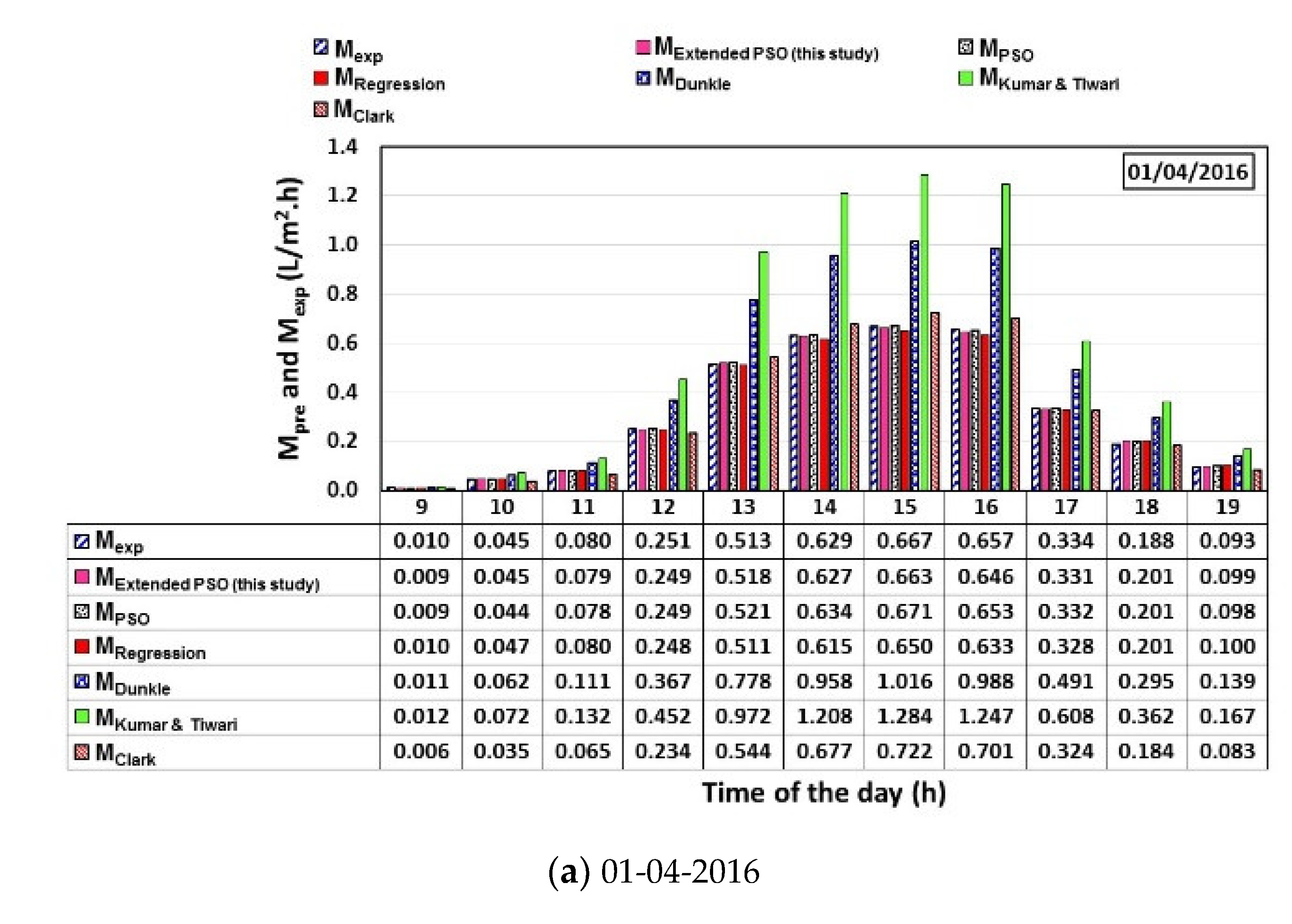
| Date | Time | Mexp (L/m2·h) | MDeveloped PSO (This Study) (L/m2·h) | MPSO (L/m2·h) | MDunkle (L/m2·h) | MRegression (L/m2·h) | MKumar & Tiwari (L/m2·h) | MClark (L/m2·h) | MDeveloped PSO (This Study) /Mexp | MPSO/Mexp | MDunkle/Mexp | MRegression /Mexp | MKumar & Tiwari/Mexp | MClark/Mexp |
|---|---|---|---|---|---|---|---|---|---|---|---|---|---|---|
| 01/04/2016 | 9:00 | 0.010 | 0.009 | 0.009 | 0.011 | 0.010 | 0.012 | 0.006 | 0.91 | 0.88 | 1.14 | 0.98 | 1.25 | 0.61 |
| 10:00 | 0.045 | 0.045 | 0.044 | 0.062 | 0.047 | 0.072 | 0.035 | 1.01 | 0.99 | 1.37 | 1.04 | 1.61 | 0.78 | |
| 11:00 | 0.080 | 0.079 | 0.078 | 0.111 | 0.080 | 0.132 | 0.065 | 0.99 | 0.97 | 1.38 | 1.01 | 1.65 | 0.81 | |
| 12:00 | 0.251 | 0.249 | 0.249 | 0.367 | 0.248 | 0.452 | 0.234 | 0.99 | 0.99 | 1.46 | 0.99 | 1.80 | 0.93 | |
| 13:00 | 0.513 | 0.518 | 0.521 | 0.778 | 0.511 | 0.972 | 0.544 | 1.01 | 1.02 | 1.52 | 1.00 | 1.89 | 1.06 | |
| 14:00 | 0.629 | 0.627 | 0.634 | 0.958 | 0.615 | 1.208 | 0.677 | 1.00 | 1.01 | 1.52 | 0.98 | 1.92 | 1.08 | |
| 15:00 | 0.667 | 0.663 | 0.671 | 1.016 | 0.650 | 1.284 | 0.722 | 0.99 | 1.01 | 1.52 | 0.97 | 1.93 | 1.08 | |
| 16:00 | 0.657 | 0.646 | 0.653 | 0.988 | 0.633 | 1.247 | 0.701 | 0.98 | 0.99 | 1.50 | 0.96 | 1.90 | 1.07 | |
| 17:00 | 0.334 | 0.331 | 0.332 | 0.491 | 0.328 | 0.608 | 0.324 | 0.99 | 0.99 | 1.47 | 0.98 | 1.82 | 0.97 | |
| 18:00 | 0.188 | 0.201 | 0.201 | 0.295 | 0.201 | 0.362 | 0.184 | 1.07 | 1.07 | 1.57 | 1.07 | 1.93 | 0.98 | |
| 19:00 | 0.093 | 0.099 | 0.098 | 0.139 | 0.100 | 0.167 | 0.083 | 1.06 | 1.05 | 1.50 | 1.07 | 1.80 | 0.89 | |
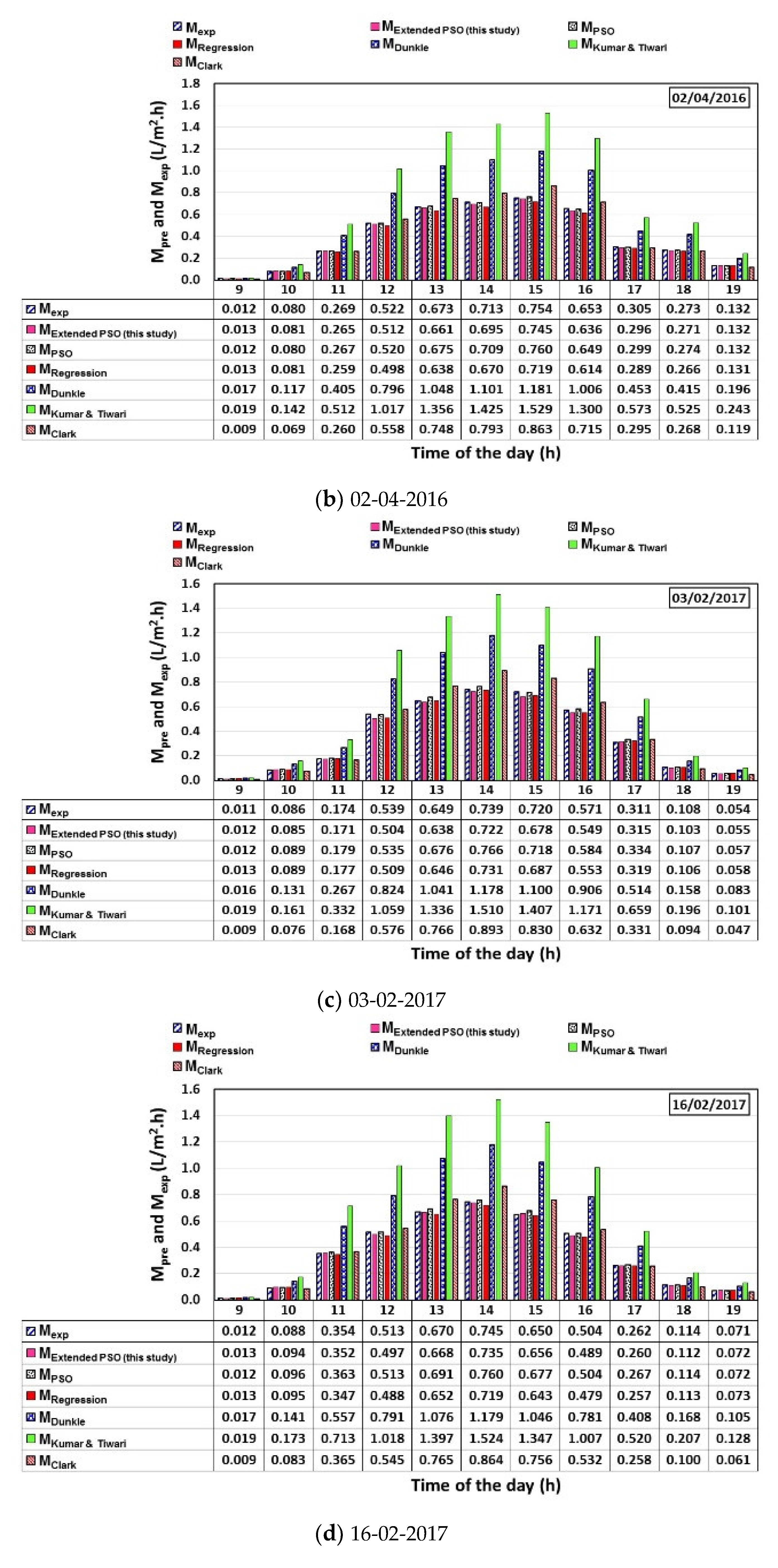
| 02/04/2016 | 9:00 | 0.012 | 0.013 | 0.012 | 0.017 | 0.013 | 0.019 | 0.009 | 1.06 | 1.03 | 1.40 | 1.11 | 1.60 | 0.75 |
| 10:00 | 0.080 | 0.081 | 0.080 | 0.117 | 0.081 | 0.142 | 0.069 | 1.01 | 1.00 | 1.46 | 1.01 | 1.78 | 0.86 | |
| 11:00 | 0.269 | 0.265 | 0.267 | 0.405 | 0.259 | 0.512 | 0.260 | 0.98 | 0.99 | 1.51 | 0.96 | 1.90 | 0.97 | |
| 12:00 | 0.522 | 0.512 | 0.520 | 0.796 | 0.498 | 1.017 | 0.558 | 0.98 | 1.00 | 1.52 | 0.95 | 1.95 | 1.07 | |
| 13:00 | 0.673 | 0.661 | 0.675 | 1.048 | 0.638 | 1.356 | 0.748 | 0.98 | 1.00 | 1.56 | 0.95 | 2.02 | 1.11 | |
| 14:00 | 0.713 | 0.695 | 0.709 | 1.101 | 0.670 | 1.425 | 0.793 | 0.97 | 0.99 | 1.54 | 0.94 | 2.00 | 1.11 | |
| 15:00 | 0.754 | 0.745 | 0.760 | 1.181 | 0.719 | 1.529 | 0.863 | 0.99 | 1.01 | 1.57 | 0.95 | 2.03 | 1.14 | |
| 16:00 | 0.653 | 0.636 | 0.649 | 1.006 | 0.614 | 1.300 | 0.715 | 0.97 | 0.99 | 1.54 | 0.94 | 1.99 | 1.10 | |
| 17:00 | 0.305 | 0.296 | 0.299 | 0.453 | 0.289 | 0.573 | 0.295 | 0.97 | 0.98 | 1.48 | 0.95 | 1.88 | 0.97 | |
| 18:00 | 0.273 | 0.271 | 0.274 | 0.415 | 0.266 | 0.525 | 0.268 | 0.99 | 1.00 | 1.52 | 0.97 | 1.92 | 0.98 | |
| 19:00 | 0.132 | 0.132 | 0.132 | 0.196 | 0.131 | 0.243 | 0.119 | 1.00 | 1.00 | 1.48 | 0.99 | 1.84 | 0.90 | |
| 03/02/2017 | 9:00 | 0.011 | 0.012 | 0.012 | 0.016 | 0.013 | 0.019 | 0.009 | 1.08 | 1.10 | 1.50 | 1.18 | 1.72 | 0.80 |
| 10:00 | 0.086 | 0.085 | 0.089 | 0.131 | 0.089 | 0.161 | 0.076 | 0.99 | 1.03 | 1.52 | 1.03 | 1.87 | 0.89 | |
| 11:00 | 0.174 | 0.171 | 0.179 | 0.267 | 0.177 | 0.332 | 0.168 | 0.98 | 1.03 | 1.53 | 1.02 | 1.91 | 0.96 | |
| 12:00 | 0.539 | 0.504 | 0.535 | 0.824 | 0.509 | 1.059 | 0.576 | 0.93 | 0.99 | 1.53 | 0.94 | 1.96 | 1.07 | |
| 13:00 | 0.649 | 0.638 | 0.676 | 1.041 | 0.646 | 1.336 | 0.766 | 0.98 | 1.04 | 1.60 | 0.99 | 2.06 | 1.18 | |
| 14:00 | 0.739 | 0.722 | 0.766 | 1.178 | 0.731 | 1.510 | 0.893 | 0.98 | 1.04 | 1.59 | 0.99 | 2.04 | 1.21 | |
| 15:00 | 0.720 | 0.678 | 0.718 | 1.100 | 0.687 | 1.407 | 0.830 | 0.94 | 1.00 | 1.53 | 0.95 | 1.95 | 1.15 | |
| 16:00 | 0.571 | 0.549 | 0.584 | 0.906 | 0.553 | 1.171 | 0.632 | 0.96 | 1.02 | 1.59 | 0.97 | 2.05 | 1.11 | |
| 17:00 | 0.311 | 0.315 | 0.334 | 0.514 | 0.319 | 0.659 | 0.331 | 1.01 | 1.08 | 1.65 | 1.03 | 2.12 | 1.07 | |
| 18:00 | 0.108 | 0.103 | 0.107 | 0.158 | 0.106 | 0.196 | 0.094 | 0.95 | 0.99 | 1.47 | 0.99 | 1.81 | 0.87 | |
| 19:00 | 0.054 | 0.055 | 0.057 | 0.083 | 0.058 | 0.101 | 0.047 | 1.02 | 1.06 | 1.54 | 1.07 | 1.86 | 0.88 | |
| 16/02/2017 | 9:00 | 0.012 | 0.013 | 0.012 | 0.017 | 0.013 | 0.019 | 0.009 | 1.05 | 1.04 | 1.41 | 1.11 | 1.62 | 0.76 |
| 10:00 | 0.088 | 0.094 | 0.096 | 0.141 | 0.095 | 0.173 | 0.083 | 1.07 | 1.09 | 1.60 | 1.08 | 1.97 | 0.94 | |
| 11:00 | 0.354 | 0.352 | 0.363 | 0.557 | 0.347 | 0.713 | 0.365 | 1.00 | 1.02 | 1.57 | 0.98 | 2.01 | 1.03 | |
| 12:00 | 0.513 | 0.497 | 0.513 | 0.791 | 0.488 | 1.018 | 0.545 | 0.97 | 1.00 | 1.54 | 0.95 | 1.98 | 1.06 | |
| 13:00 | 0.670 | 0.668 | 0.691 | 1.076 | 0.652 | 1.397 | 0.765 | 1.00 | 1.03 | 1.61 | 0.97 | 2.08 | 1.14 | |
| 14:00 | 0.745 | 0.735 | 0.760 | 1.179 | 0.719 | 1.524 | 0.864 | 0.99 | 1.02 | 1.58 | 0.97 | 2.05 | 1.16 | |
| 15:00 | 0.650 | 0.656 | 0.677 | 1.046 | 0.643 | 1.347 | 0.756 | 1.01 | 1.04 | 1.61 | 0.99 | 2.07 | 1.16 | |
| 16:00 | 0.504 | 0.489 | 0.504 | 0.781 | 0.479 | 1.007 | 0.532 | 0.97 | 1.00 | 1.55 | 0.95 | 2.00 | 1.06 | |
| 17:00 | 0.262 | 0.260 | 0.267 | 0.408 | 0.257 | 0.520 | 0.258 | 0.99 | 1.02 | 1.56 | 0.98 | 1.99 | 0.98 | |
| 18:00 | 0.114 | 0.112 | 0.114 | 0.168 | 0.113 | 0.207 | 0.100 | 0.98 | 1.00 | 1.47 | 0.99 | 1.82 | 0.88 | |
| 19:00 | 0.071 | 0.072 | 0.072 | 0.105 | 0.073 | 0.128 | 0.061 | 1.01 | 1.02 | 1.48 | 1.03 | 1.80 | 0.86 | |
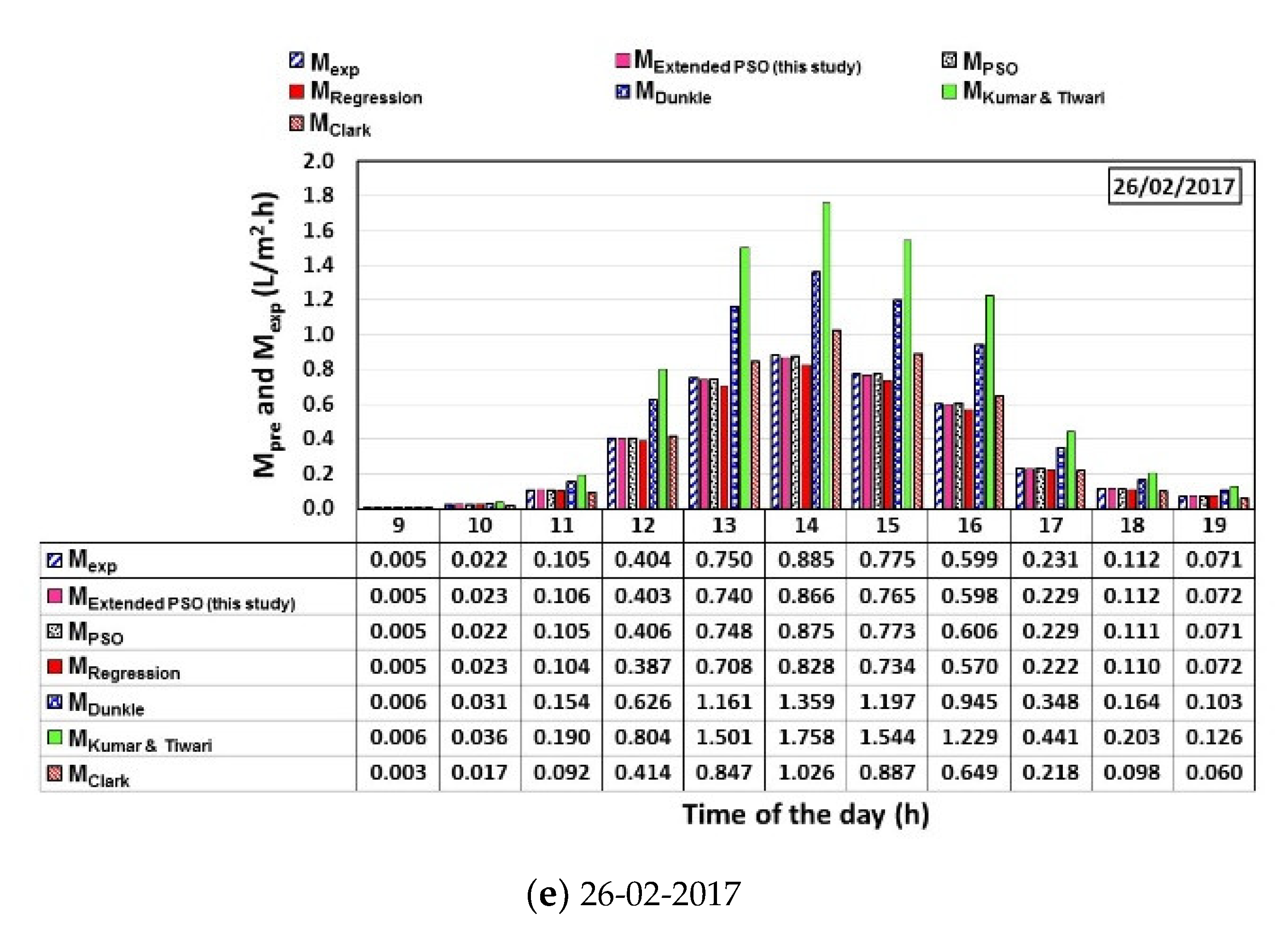
| 26/02/2017 | 9:00 | 0.005 | 0.005 | 0.005 | 0.006 | 0.005 | 0.006 | 0.003 | 0.96 | 0.90 | 1.16 | 1.03 | 1.26 | 0.61 |
| 10:00 | 0.022 | 0.023 | 0.022 | 0.031 | 0.023 | 0.036 | 0.017 | 1.04 | 1.01 | 1.40 | 1.06 | 1.63 | 0.77 | |
| 11:00 | 0.105 | 0.106 | 0.105 | 0.154 | 0.104 | 0.190 | 0.092 | 1.01 | 1.00 | 1.47 | 0.99 | 1.81 | 0.88 | |
| 12:00 | 0.404 | 0.403 | 0.406 | 0.626 | 0.387 | 0.804 | 0.414 | 1.00 | 1.01 | 1.55 | 0.96 | 1.99 | 1.03 | |
| 13:00 | 0.750 | 0.740 | 0.748 | 1.161 | 0.708 | 1.501 | 0.847 | 0.99 | 1.00 | 1.55 | 0.94 | 2.00 | 1.13 | |
| 14:00 | 0.885 | 0.866 | 0.875 | 1.359 | 0.828 | 1.758 | 1.026 | 0.98 | 0.99 | 1.54 | 0.94 | 1.99 | 1.16 | |
| 15:00 | 0.775 | 0.765 | 0.773 | 1.197 | 0.734 | 1.544 | 0.887 | 0.99 | 1.00 | 1.54 | 0.95 | 1.99 | 1.14 | |
| 16:00 | 0.599 | 0.598 | 0.606 | 0.945 | 0.570 | 1.229 | 0.649 | 1.00 | 1.01 | 1.58 | 0.95 | 2.05 | 1.08 | |
| 17:00 | 0.231 | 0.229 | 0.229 | 0.348 | 0.222 | 0.441 | 0.218 | 0.99 | 0.99 | 1.51 | 0.96 | 1.91 | 0.94 | |
| 18:00 | 0.112 | 0.112 | 0.111 | 0.164 | 0.110 | 0.203 | 0.098 | 1.00 | 0.99 | 1.46 | 0.98 | 1.81 | 0.87 | |
| 19:00 | 0.071 | 0.072 | 0.071 | 0.103 | 0.072 | 0.126 | 0.060 | 1.01 | 1.00 | 1.45 | 1.01 | 1.77 | 0.84 | |
| STD | 0.031 | 0.032 | 0.079 | 0.054 | 0.161 | 0.142 | ||||||||
| Mean | 0.994 | 1.013 | 1.519 | 0.993 | 1.906 | 0.992 | ||||||||
| CoV | 3.1% | 3.1% | 5.2% | 5.4% | 8.5% | 14.3% | ||||||||
| Model | Predicted Versus Experimental | ||
|---|---|---|---|
| R | PI | RRMSE (%) | |
| Regression | 0.9989 | 0.0308 | 6.15 |
| Kumar and Tiwari’s | 0.9980 | 0.7072 | 141.37 |
| Clark’s | 0.9956 | 0.0891 | 17.81 |
| Dunkle’s | 0.9988 | 0.3935 | 78.68 |
| PSO-HYSS | 0.9991 | 0.0173 | 3.46 |
| Developed PSO-HYSS (this study) | 0.9992 | 0.0141 | 2.81 |
| Item | Formulas | Conditions | Developed PSO–HYSS (Current Study) | PSO–HYSS | Regression | Dunkle’s | Kumar and Tiwari’s | Clark’s |
|---|---|---|---|---|---|---|---|---|
| 1 | R, Equation (30) | R more than 0.8 | 0.9992 | 0.9991 | 0.9989 | 0.9988 | 0.9980 | 0.9956 |
| 0.9830 | 1.0084 | 0.962 | 1.552 | 1.992 | 1.110 | |||
| 3 | 1.0170 | 0.9914 | 1.039 | 0.644 | 0.501 | 0.899 | ||
| 4 | Rm more than 0.5 | 0.9957 | 0.9727 | 0.944 | 0.413 | 0.178 | 0.843 | |
| 5 | 0.00000 | −0.00071 | 0.00288 | 0.81633 | 2.59689 | 0.02558 | ||
| 6 | −0.00001 | −0.00070 | 0.00300 | 0.34419 | 0.67563 | 0.02372 |
Publisher’s Note: MDPI stays neutral with regard to jurisdictional claims in published maps and institutional affiliations. |
© 2022 by the authors. Licensee MDPI, Basel, Switzerland. This article is an open access article distributed under the terms and conditions of the Creative Commons Attribution (CC BY) license (https://creativecommons.org/licenses/by/4.0/).
Share and Cite
Al-Sulttani, A.O.; Ahsan, A.; Al-Bakri, B.A.R.; Hason, M.M.; Daud, N.N.N.; Idrus, S.; Alawi, O.A.; Macioszek, E.; Yaseen, Z.M. Double-Slope Solar Still Productivity Based on the Number of Rubber Scraper Motions. Energies 2022, 15, 7881. https://0-doi-org.brum.beds.ac.uk/10.3390/en15217881
Al-Sulttani AO, Ahsan A, Al-Bakri BAR, Hason MM, Daud NNN, Idrus S, Alawi OA, Macioszek E, Yaseen ZM. Double-Slope Solar Still Productivity Based on the Number of Rubber Scraper Motions. Energies. 2022; 15(21):7881. https://0-doi-org.brum.beds.ac.uk/10.3390/en15217881
Chicago/Turabian StyleAl-Sulttani, Ali O., Amimul Ahsan, Basim A. R. Al-Bakri, Mahir Mahmod Hason, Nik Norsyahariati Nik Daud, S. Idrus, Omer A. Alawi, Elżbieta Macioszek, and Zaher Mundher Yaseen. 2022. "Double-Slope Solar Still Productivity Based on the Number of Rubber Scraper Motions" Energies 15, no. 21: 7881. https://0-doi-org.brum.beds.ac.uk/10.3390/en15217881