Monopolar Grounding Fault Location Method of DC Distribution Network Based on Improved ReliefF and Weighted Random Forest

Abstract

Compared with the pole-to-pole short circuit, the fault characteristics are not obvious when a monopolar grounding fault occurs in a DC distribution network, and it is difficult to locate the fault accurately. To solve this problem, this paper proposes a fault location method based on improved ReliefF and Weighted random forest (WRF). The 24 time and frequency-domain fault features of the postfault aerial mode current are calculated, and the most useful features are selected to form the optimal feature subset for input to the fault location estimator. In this paper, the ReliefF algorithm is utilized for automatic feature selection and obtaining the weights of features. In addition, the WRF algorithm is used to build the fault location estimator. Considering the fault location, fault resistance, noise and time window length, the Matlab/Simulink simulation platform is used to simulate the fault situation and compare it with other algorithms. The simulation results show that the average positioning error of the fault location method is less than 0.1%, which is not affected by the fault resistance and has strong robustness.

1. Introduction

With the rapid development of renewable energy, energy storage devices and various new flexible loads, flexible DC distribution networks have received extensive attention from experts and scholars due to their unique advantages [1,2,3,4]. The flexible DC distribution network is not limited by synchronization stability and has the advantages of large transmission capacity, high power quality and flexible control.

The DC line is generally composed of underground cables, so it is difficult to locate faults through the traditional manual method. The faults of DC cables are generally permanent rather than transient. The DC system has low inertia, and the fault transition is rapid, while the superimposed output of multiple converter stations after the fault makes the consequences of the fault more serious. From the perspective of power system safety and stability, the fault must be quickly located. The rapid and accurate fault location is one of the key points to ensure its reliable operation and rapid recovery [5].

However, due to the late beginning, the fault location technology of a flexible DC distribution network based on a voltage source converter (VSC) has not been fully studied, and there is no better plan, especially for DC monopolar grounding fault location. On the one hand, the potential risk of rapidly rising fault currents in low fault resistance in effectively grounded distribution networks leads to a significant limitation of available information and measurement time for fault location methods [6]. On the other hand, when a high fault resistance grounding fault occurs, the weak fault characteristic information will become a serious test of the fault ranging method. There is a lack of research on this issue [7]. At the same time, the distribution lines of the DC distribution network are short, and the network structure is complex. When applying some fault location methods of HVDC, such as the traveling wave method, the adaptability is greatly reduced due to problems such as the traveling wave head identification and extremely high sampling frequency requirements.

Existing research on fault location for flexible DC distribution networks based on voltage source converter (VSC) mainly focuses on short circuits between poles, and the topology is mainly radial connection or tree connection with a simple structure. The techniques for short-circuit fault location in DC distribution networks are mainly divided into three categories: fault analysis method, traveling wave method and artificial intelligence method. The fault analysis method performs fault location based on the functional relationship between the collected voltage, the current or its characteristic parameters and the fault distance. This method is simple in principle and low in sampling frequency and has high research and application value in medium and low voltage DC distribution networks. Considering the drawbacks of the mentioned single-terminal protections, the literature [8] proposes a current waveform curvature based on a protection scheme. To compensate for the shortcomings of the existing two-terminal fault location methods and to obtain accurate fault location information, a two-terminal fault ranging model based on the time-domain differential equations of RL lines was established in [9]. However, the defects of the RL model itself make the method not suitable for networks with complex topology. In [10], the scholar proposes to use the time difference between two consecutive reflected wave heads for fault location on DC transmission lines, named the traveling wave method for fault location. However, as the identification of traveling wave heads is difficult and requires high sampling frequency, the investment in related equipment is high, which limits the development of the traveling wave method in DC distribution systems [11,12,13]. As scholars pay more and more attention to machine learning, some fault location schemes based on intelligent algorithms have gradually become the focus of research. In [14], the authors carry out parameter identification of fault locations of DC distribution lines under different fault types based on genetic algorithms. The improved fault location method based on clustering and iterating algorithms is proposed in reference [15], which eliminates the negative influence of signal dimension fluctuation and false spectrum peak phenomenon of multiple signal classification significantly. Reference [16] uses a particle swarm algorithm for parameter identification and uses double-terminal power to obtain the fault location. The random forest algorithm has strong performance in processing high-dimensional input feature vectors. The authors in [17] propose an intelligent method for fault location in HVDC systems using single terminal post-fault voltage signals with a feature selection tool and a random forest estimator. This method has high practical value, but the redundancy of feature subsets is not considered, which may lead to unreliable fault location results.

The main contributions of this paper are listed as follows:

• When a monopolar grounding short-circuit occurs in DC distribution lines, we construct 24 time and frequency-domain fault characteristics using the aerial mode current at the single terminal of the line.
• In this paper, the limited coefficient q is introduced to solve the shortcomings of the ReliefF algorithm in application and combined with the Pearson correlation coefficient method to automatically screen the optimal feature subset. The optimal subset and feature weight are calculated by the improved ReliefF algorithm, and the average value of the weights is taken as the final weight value. The optimal feature subset containing the weight coefficient can be obtained. The weight coefficient can continue to be used to improve the performance and fault location accuracy of the WRF algorithm in subsequent steps.
• The weighted random forest algorithm proposed in this paper mainly improves the traditional random forest algorithm in two aspects. On the one hand, considering that the improved ReliefF can obtain the specific values of the feature weight, it can be combined with the RF algorithm to form a weighted random forest algorithm, which can improve the accuracy of the model in a targeted manner. On the other hand, using the loop statement to find the values of mtry and ntree with the best model fit makes the fault location scheme more accurate. Combining the improved ReliefF with the RF, the features are no longer selected randomly, but the optimal feature subset is selected for the dataset in advance. This improvement reduces the dimensionality of the features in its input RF and eliminates redundant features, thereby greatly reducing the computation time and improving the accuracy.
• The simulation validation shows that the improved WRF algorithm has high accuracy under various conditions when applied to fault location in a DC distribution network. It has strong anti-fault resistance and anti-noise capability within a certain time window and has strong adaptability. The principle of the method is simple; only local measurement is required, no need to send and synchronize information at both ends, which greatly reduces the management and investment costs of sampling equipment and has strong engineering practicability.

2. Multiple Fault Characteristics and Optimal Feature Selection Algorithm

2.1. Monopolar Grounding Fault in a DC Distribution Network

The topologies of DC distribution systems mainly include radial, hand-in-hand and ring. A ring DC network has multiple terminals, so the topology and fault protection strategies are relatively complex. Moreover, the new energy sources such as photovoltaic and wind power increase its diversity [4]. At the same time, the ring DC network not only has the advantages of short restoration time and high reliability of power supply, but also can be widely used in the new power system. Therefore, this paper develops a six-terminal ring DC distribution network model as shown in Figure 1, which can be used to study the proposed fault location method. Where A-F are the DC buses.

The equivalent circuit of the DC line when monopolar grounding occurs is shown in Figure 2.

The fault feature of the positive pole-to-ground and negative pole-to-ground are symmetrical, so this paper takes the former as an example to study the monopolar grounding fault location method in the DC distribution system.

Unlike the pole-to-pole, the short-circuit fault must be eliminated before the voltage of capacitance crosses the zero-point. The monopolar grounding fault eventually enters the voltage recovery phase. The DC voltage gradually returns to normal, and the nonfaulty pole undertakes the short-term unipolar operation of the DC system to gain time for fault elimination. However, because the fault characteristics are not obvious, it is more difficult to accurately locate the fault.

In the bipolar DC distribution system, due to the coupling of the positive and negative parameters, the currents are first converted into aerial mode current and zero mode current components according to the Karenbauer transformation [18]:

$$\left[\begin{array}{c}{i}_1\\ i_0\end{array}\right]{=S}^{-1}\left[\begin{array}{c}{i}_p\\ i_n\end{array}\right]=\frac{\sqrt{2}}{2}\left[\begin{array}{cc}1& -1\\ 1& 1\end{array}\right]\left[\begin{array}{c}{i}_p\\ i_n\end{array}\right]$$

(1)

where i_p and i_n represent the positive and negative current of the DC line, respectively, and i₁ and i₀ represent the aerial mode and zero mode current of the DC line, respectively. The positive direction of the aerial mode component is the same as the specified positive direction of the current, and the positive direction of the zero mode component is specified to flow from the DC bus to the DC line.

The Karenbauer transformation matrix is:

$$S=\frac{\sqrt{2}}{2}\left[\begin{array}{cc}1& 1\\ -1& 1\end{array}\right]$$

(2)

2.2. Multiple Fault Characteristics

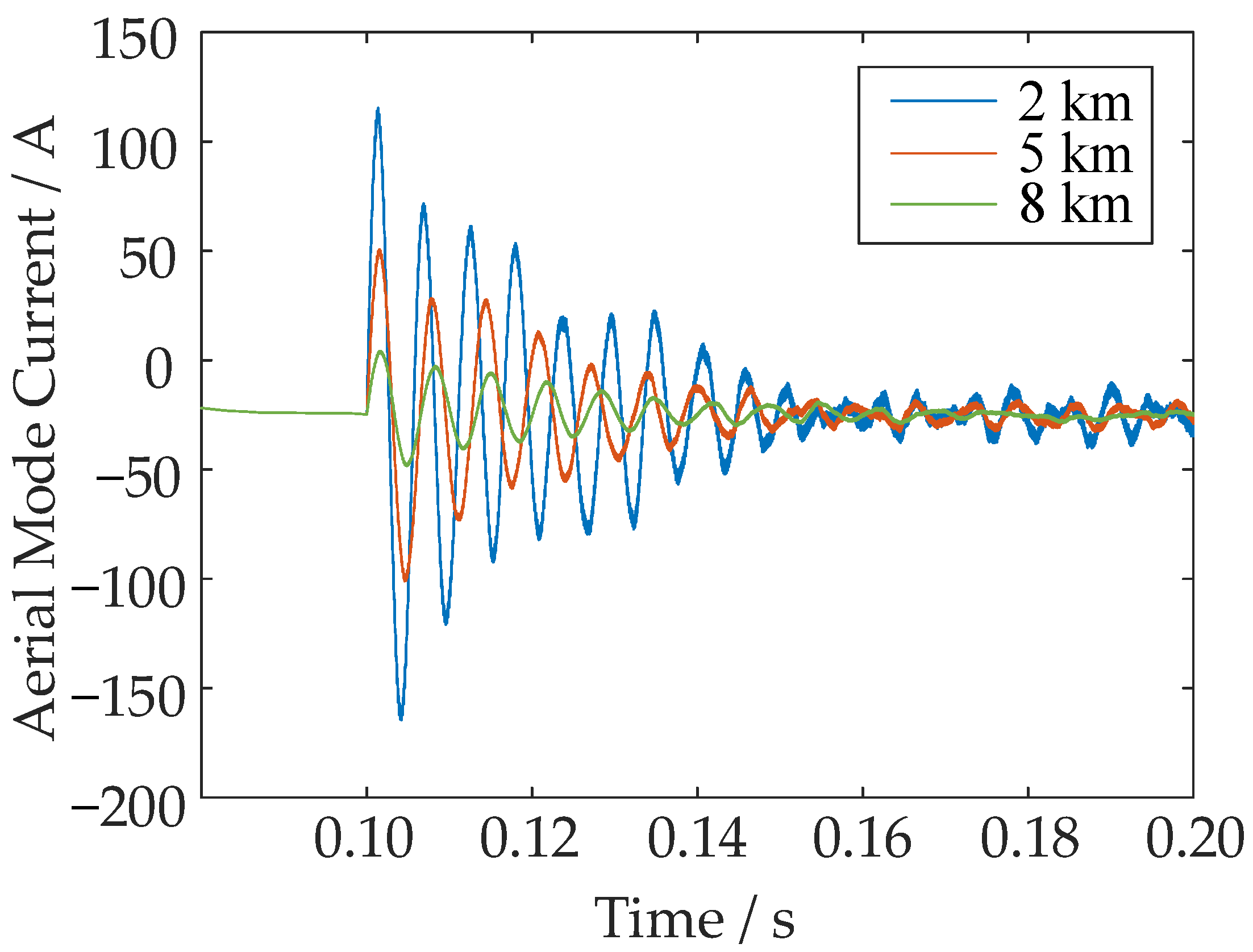
For Line 1 of the six-terminal DC distribution system shown in Figure 1, the positive pole-to-ground fault occurs at different positions from the left-end converter. The aerial mode current measured at bus A is shown in Figure 3.

When a fault occurs in a DC cable, the system gradually recovers to a stable state through a transient process. The fault transient signals are generated from the fault point to both terminals of the cable during the system transient. The normal operation of the system contains almost exclusively only the DC components, but the fault transient process contains signals of various frequencies. Moreover, the transient signal contains a lot of fault information, from which effective fault characteristics can be obtained [19].

It can be inferred from Figure 3 that the oscillation and frequency content of the aerial mode current will change with the fault location. There is a certain correspondence between them, which is difficult to express by a specific mathematical formula. From the theoretical research and simulation verification, it is known that the aerial mode current measured for a period of time after the fault occurs is a vibration signal. The original statistical characteristics of the vibration signal can be divided into two categories: time-domain statistical characteristics and frequency-domain statistical characteristics.

In order to ensure the rationality of the characteristics indicators and the credibility of the results, this manuscript extracts 11 time-domain features (T₁–T₁₁) and 13 frequency-domain features (T₁₂–T₂₄) of the aerial mode fault current, a total of 24 common indicators of vibration signal in statistics as the fault features as shown in

Table 1. Multi-domain feature parameters.

No.	Formula	No.	Formula	No.	Formula	No.	Formula
1	$T_1=\frac{{\displaystyle \sum _{n=1}^{N}x(n)}}{N}$	7	$T_7=\frac{{\displaystyle \sum _{n=1}^N{(x(n) - T_1)}^4}}{(N - 1)T_2^4}$	13	$T_{13}=\frac{{\displaystyle \sum _{k=1}^K{(s(k) - T_{12})}^2}}{K - 1}$	19	$T_{19}=\sqrt{\frac{{\displaystyle \sum _{k=1}^K{f}_k^{4}s(k)}}{{\displaystyle \sum _{k=1}^K{f}_k^{2}s(k)}}}$
2	$T_2=\sqrt{\frac{{\displaystyle \sum _{n=1}^N{(x(n) - T_1)}^2}}{N - 1}}$	8	$T_8=\frac{T_5}{T_4}$	14	$T_{14}=\frac{{\displaystyle \sum _{k=1}^K{(s(k) - T_{12})}^3}}{K{(\sqrt{T_{13}})}^3}$	20	$T_{20}=\frac{{\displaystyle \sum _{k=1}^K{f}_k^{2}s(k)}}{\sqrt{{\displaystyle \sum _{k=1}^{K}s(k){\displaystyle \sum _{k=1}^K{f}_k^{4}s(k)}}}}$
3	$T_3={(\frac{{\displaystyle \sum _{n=1}^N\sqrt{\left|x(n)\right|}}}{N})}^2$	9	$T_9=\frac{T_5}{T_3}$	15	$T_{15}=\frac{{\displaystyle \sum _{k=1}^K{(s(k) - T_{12})}^4}}{{\mathit{KT}}_{13}^2}$	21	$T_{21}=\frac{T_{17}}{T_{16}}$
4	$T_4=\sqrt{\frac{{\displaystyle \sum _{n=1}^{N}x{(n)}^2}}{N}}$	10	$T_{10}=\frac{T_4}{\frac{1}{N}{\displaystyle \sum _{n=1}^N\left|x(n)\right|}}$	16	$T_{16}=\frac{{\displaystyle \sum _{k=1}^K{f}_{k}s(k)}}{{\displaystyle \sum _{k=1}^{K}s(k)}}$	22	$T_{22}=\frac{{\displaystyle \sum _{k=1}^K{{(f}_k - T_{16})}^{3}s(k)}}{{\mathit{KT}}_{17}^3}$
5	$T_5=\mathit{max}\left|x(n)\right|$	11	$T_{11}=\frac{T_5}{\frac{1}{N}{\displaystyle \sum _{n=1}^N\left|x(n)\right|}}$	17	$T_{17}=\sqrt{\frac{{\displaystyle \sum _{k=1}^K{{(f}_k - T_{16})}^{2}s(k)}}{K}}$	23	$T_{23}=\frac{{\displaystyle \sum _{k=1}^K{(f_k - T_{16})}^{4}s(k)}}{{\mathit{KT}}_{17}^4}$
6	$T_6=\frac{{\displaystyle \sum _{n=1}^N{(x(n) - T_1)}^3}}{(N - 1)T_2^3}$	12	$T_{12}=\frac{{\displaystyle \sum _{k=1}^{K}s(k)}}{K}$	18	$T_{18}=\sqrt{\frac{{\displaystyle \sum _{k=1}^K{f}_k^{2}s(k)}}{{\displaystyle \sum _{k=1}^{K}s(k)}}}$	24	$T_{24}=\frac{{\displaystyle \sum _{k=1}^K(f_k - T_{16}{)}^{2}s(k)}}{K\sqrt[4]{T_{17}}}$

Where x(n) is the time-domain signal sequence, n = 1, 2, …, N; N is the number of sample points; s(k) is the spectrum obtained by discrete Fourier transform (DFT) of the time-domain signal x(n), k = 1, 2, …, K; K is the number of spectral lines; f_k is the frequency value of the kth spectral line.

.

The statistical significance of each feature quantity is as follows:

• Time-domain: T₁: average value; T₂: standard deviation; T₃: square root amplitude; T₄: root mean square; T₅: peak value; T₆: skewness; T₇: kurtosis; T₈: crest factor; T₉: clearance indicator; T₁₀: shape indicator; T₁₁: impulse indicator.
• Frequency-domain: T₁₂: central frequency; T₁₃: variance frequency; T₁₄: skewness frequency; T₁₅: peak value frequency; T₁₆: gravity frequency; T₁₇: standard deviation frequency; T₁₈: root mean square frequency; T₁₉: mean square frequency; T₂₀: waveform stability factor; T₂₁: coefficient of variation; T₂₂: skewness frequency; T₂₃: kurtosis frequency; T₂₄: square root ratio.

Through the comprehensive representation of these 24 features, the fault aerial mode current can be fully described. Thereby, subtle differences between different fault current vibration signals corresponding to different fault locations can be distinguished.

2.3. Optimal Feature Subset Selection

2.3.1. ReliefF Algorithm

In an intelligent algorithm, feature pre-selection is one of the preprocessing stages to improve the accuracy and performance of artificial intelligence. Relief is a classic filter feature selection algorithm, but it is limited to binary problems and cannot deal with noise and missing values in the data.

Kononeill proposed the ReliefF algorithm for multi-classification problems based on the Relief idea and expressed the importance of features by setting a “correlation statistic”. The essence of correlation statistics is to measure the ability of the feature to perform “intra-class aggregation and inter-class divergence”, and it is an important measure of the degree of feature importance [20]. According to the correlation of each feature and category, the features are assigned weights of different sizes, and the features are sorted according to the size of the weight. The larger the feature weight, the higher the correlation of the feature will be. During feature selection, features with smaller weights can be removed according to the set threshold to form the optimal feature subset.

The specific method for selecting multiple fault features in the time and frequency-domain of aerial mode current based on the ReliefF algorithm is as follows:

• Randomly select a sample R_i from the feature ensemble training set.
• Find the K nearest neighbor samples H_j and M_j (j = 1, 2, …, K) from the set of samples of both the same and different classes as sample R_i, respectively.
• Use the K-nearest neighbors (KNN) idea to iterate repeatedly on each feature dimension and update the weight W(T_p) of each feature T_p (p = 1, 2, …,24) according to Formula (3).

$$W(T_p)=W(T_p)-\frac{1}{\mathit{mK}}{\displaystyle \sum _{j=1}^{K}d}(T_p,X,H_j)+\frac{1}{\mathit{mK}}\frac{P(c)}{1-P(c)}{\displaystyle \sum _{j=1}^{K}d}(T_p,X,M_j)$$

(3)

where m is the number of algorithm iterations. P(c) is the probability of class c samples in the training set, d(T_p, X, H_j) presents the distance between sample X and sample H_j on multiple features T_p, and d(T_p, X, M_j) presents the distance between sample X and sample M_j on multiple features T_p, which is calculated by Formulas (4) and (5).

$$d(T_p,X,H_j)=\frac{\left|V(T_p,X)-V(T_p,H_j)\right|}{\max (T_p)-\min (T_p)}$$

(4)

$$d(T_p,X,M_j)=\frac{\left|V(T_p,X)-V(T_p,M_j)\right|}{\max (T_p)-\min (T_p)}$$

(5)

where V(T_p, A) denotes the value of the characteristic T_p of sample A. A denotes X, H_j or M_j.

4.

Repeat the above process m times, and calculate the average weight as the final assignment result of the feature.

5.

After the iterations are completed, the weights W(T_p) of the features are ranked from largest to smallest, and the top-ranked features are extracted according to the set weight threshold α to form the feature subset.

2.3.2. Deficiency and Improvement Strategy

The ReliefF algorithm has the advantages of high operational efficiency, no restriction on data types, strong anti-noise ability and suitability for multi-feature classification, but there are still the following shortcomings in practice:

• The random selection of samples may lead to the selection of edge samples or interference samples with wild values, which may cause errors when updating the feature weights. At the same time, random selection does not guarantee every small category sample is selected, and the number of samples selected is uneven. These factors will affect the stability and accuracy of feature selection.
• The algorithm is sensitive to the number of iterations m and the number of nearest neighbor samples K. Different combinations of parameters may lead to different assignment results. It is necessary to consider the actual classification situation and assign values determined by m and K.
• Only the contribution of different features to the classification can be calculated, and the subset of features formed does not exclude the possible redundant features.

To address the first two shortcomings, this paper adds a limiting coefficient q and proposes an improved ReliefF optimal feature subset selection method. On the premise that the total number of samplings remains unchanged, the number of repeated samplings of a single sample is limited by the limitation coefficient q. The value of q represents the maximum number of times a single sample can be selected, which needs to be decided according to the number of input features. If the value of q is too large, it may lead to the repeated sampling of a single sample, and the probability of small class samples being selected is low. If the value of q is too small, it may lead to insufficient iteration, the optimal solution is not obtained, and the result is unreliable. For the 24 time and frequency-domain multiple features constructed in Section 2.2, q = 3 is taken here. This measure can ensure the equality of each sample under the limited number of sampling times and improve the reliability of the results. The total sampling time m is determined by the product of q and the number of features.

For redundant features that may exist in feature subsets, the most common processing method at present is to pre-eliminate some features with high similarity by calculating the cosine similarity between features, and then select the optimal subset to calculate the weight. The cosine similarity calculation formula of the vectors X = (X₁, X₂, …, X_n) and Y = (Y₁, Y₂, …, Y_n) is given by (6).

$$\cos (X,Y)=\frac{{\displaystyle \sum _{i=1}^n{X}_i\cdot Y_i}}{\sqrt{{\displaystyle \sum _{i=1}^n{X}_i^2}}\cdot \sqrt{{\displaystyle \sum _{i=1}^n{Y}_i^2}}}$$

(6)

As can be seen in (6), the cosine similarity uses the cosine value of the angle between two vectors in the vector space to measure the difference between two vectors, so it only evaluates the spatial correlation, while ignoring the numerical correlation of features. In order to improve the reliability of correlation evaluation, this paper uses the Pearson correlation coefficient (PCC) to calculate the correlation between features. The Pearson correlation coefficient calculates the cosine similarity based on the centralized processing of the two groups of data, which can better measure the similarity of the details rather than the correlation of the symbols. The value range of PCC(X, Y) is (−1, 1), and the closer to 1, the higher the positive correlation between the two groups of data. The PCC between vectors X = (X₁, X₂, …, X_n) and Y = (Y₁, Y₂, …, Y_n) is given by (7).

$$\mathit{PCC}(X,Y)=\frac{{\displaystyle \sum _{i=1}^n{(X}_i-\overline{X})\cdot {(Y}_i-\overline{Y})}}{\sqrt{{\displaystyle \sum _{i=1}^n{(X}_i}-\overline{X}{)}^2}\cdot \sqrt{{\displaystyle \sum _{i=1}^n{(Y_i-\overline{Y})}^2}}}$$

(7)

where $\overline{X}$ and $\overline{Y}$ correspond to the average value of features X and Y, respectively. After calculating PCC(X, Y), the hypothesis test is used to judge whether the correlation between features is significant, and the result is presented as the p-value.

The p-value is a numerical standard to measure whether the correlation coefficient result is significant. If the p-value between two features is greater than a certain value, it means that the PCC result between them is not significant. Even if the PCC is close to 0, these two features may be redundant features of each other. If the p-value is less than a certain value, it means that the calculated correlation coefficient result is significant, and PCC can be used to characterize the degree of correlation between them.

2.3.3. Process of Improved ReliefF Algorithm

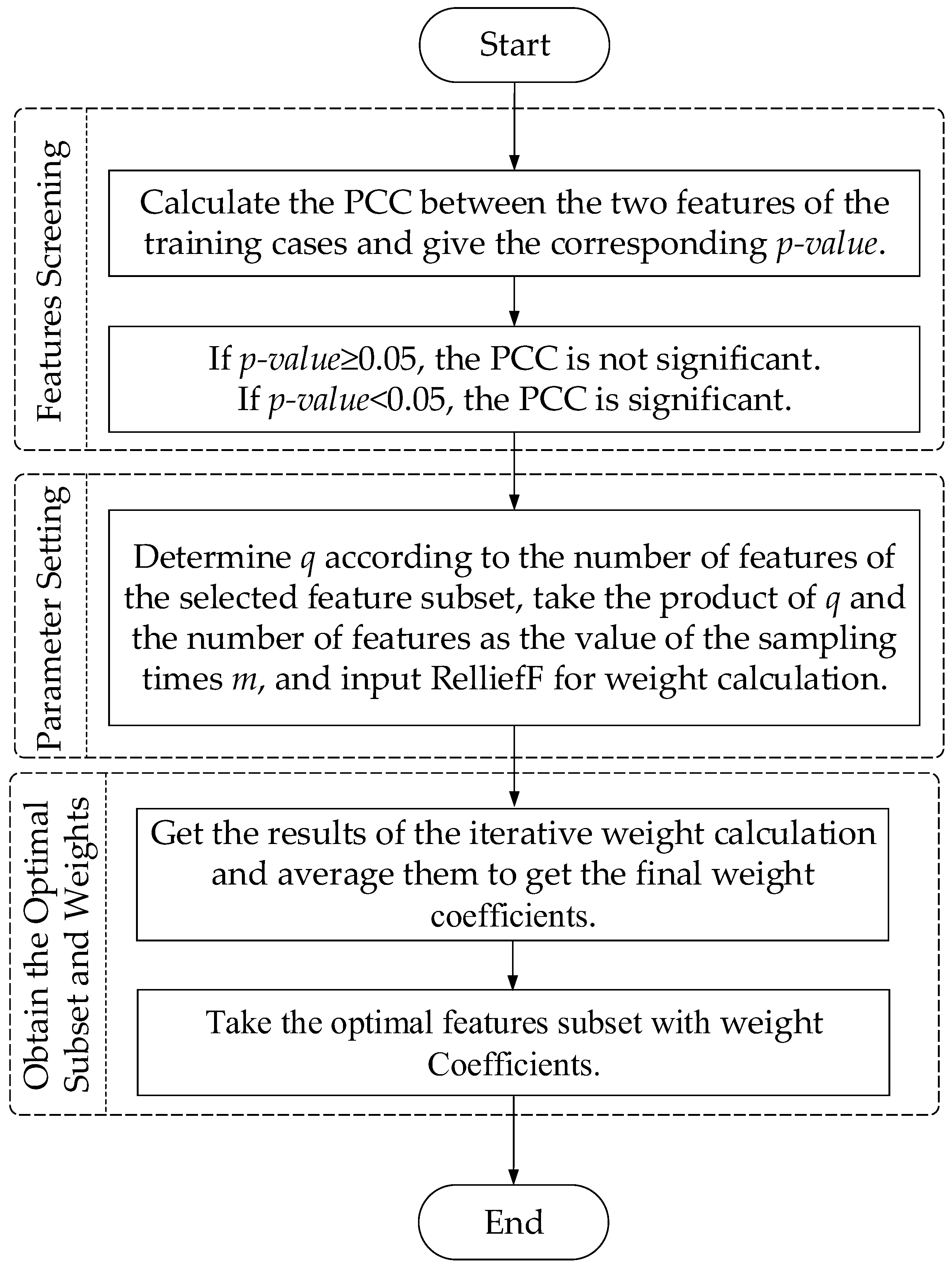
The steps of the improved ReliefF algorithm to select the optimal feature subset are shown in Figure 4.

• The process of feature subset selection mainly includes the following three steps: Calculate the PCC between each feature in the training set and select features based on whether the p-value is greater than 0.05. If the p-value ≥ 0.05, it means that there is no significant correlation between them, even if the PCC is close to 0, the two features cannot be selected together. Otherwise, if the p-value < 0.05, the calculated correlation coefficient result is significant.
• Determine the limit coefficient q according to the number of feature elements of the remaining feature subsets, and then use the product of q and the number of features as the sampling times. Then input it into the ReliefF model for feature weight calculation
• The average of the feature weights are taken as the final weight value, and the feature values in the feature subset are multiplied by the corresponding final weights to obtain the optimal feature subset containing the weight coefficients. The weight coefficient can continue to be used to improve the performance and fault location accuracy of the subsequent RF algorithm [21].

3. Weighted Random Forest

3.1. Random Forest Algorithm

Random forest (RF) is a classical ensemble learning algorithm. By combining multiple decision trees through bootstrap aggregating (bagging), this algorithm can effectively solve the problem of low accuracy of a single model in dealing with classification and regression problems and greatly improve the generalization ability of the model. It has been widely used in various fields.

RF is mainly divided into the following steps when dealing with classification and regression problems:

• Use bootstrap resampling to extract an equal number of samples with replacement from the training set and use them as the training set for a single decision tree.
• The decision tree starts to split from the top to the bottom of the node. When splitting, a portion of the features m (m is a positive integer less than M) from the M explanatory variables in the sample is extracted as a sub-feature. Then, select an optimal feature from the sub-feature m for node splitting.
• Each decision tree is repeatedly split according to step 2 until the node cannot be split.
• A total of N decision trees are generated through steps 2 and 3. Each decision tree is fitted with a weak learner, and the optimal fitting result is finally selected by voting and output as the result.

The RF algorithm uses bagging to integrate decision trees, which improves the accuracy and stability of decision tree classification and regression. However, the algorithm takes a long time to process high-latitude datasets, and the model may overfit. Therefore, the algorithm needs to be optimized accordingly.

3.2. Weighted Random Forest

The improved ReliefF algorithm proposed in Section 2 is used to replace the random selection of features in the RF algorithm, and the optimal feature subset is selected in advance. This improvement can eliminate redundant features and reduce the dimensionality of the features, thereby greatly reducing the computation time and improving the model accuracy.

The optimization and improvement of the RF algorithm in this paper mainly include two aspects. On the one hand, the improved ReliefF can obtain the specific weight of the features, which can be combined with the RF algorithm to form the WRF algorithm. The prediction accuracy of the model improved. On the other hand, the computational accuracy of the WRF depends to a large extent on two parameters: e and ntree. The former is the number of attributes pre-selected when the decision tree nodes are divided, and the latter is the total number of decision trees.

To determine the optimal model of WRF, loop statements were used to find the values of mtry and ntree with the best model fit, so that the fault location scheme has higher accuracy.

The process of the combined WRF algorithm is as follows:

• Use the improved ReliefF algorithm to filter out the optimal subset of features in the original training set and generate the corresponding weights for the features.
• Build the WRF fault location model, then find and set the optimal mtry and ntree values by using a loop statement.
• Multiply the calculated weights with the feature values and input them into the WRF model for fitting. Calculate the error rate of out of bag (OOB) data and evaluate the goodness of fit of the model.

The WRF combined with the improved ReliefF can effectively improve the fit accuracy of features and achieve higher computational efficiency.

4. Monopolar Grounding Fault Location Method Based on Improved ReliefF and WRF

Based on the above analysis, this paper proposes an improved ReliefF and WRF algorithm for a multi-feature fault location method for monopolar grounding in the DC distribution network. The overall process is shown in Figure 5, and the specific steps are as follows:

• Start to record the current and voltage data at the observation point for 100 ms when the relay protection device detects the monopolar grounding in the DC distribution line. The Karenbauer transform was performed on the recorded data to calculate the aerial mode currents.
• According to the aerial mode current, 11 time-domain features and 13 frequency-domain features are calculated to form the original multi-feature parameter table.
• The PPC is used to eliminate the redundant features in the original multi-feature parameter table.
• The de-redundant features are input into the improved ReliefF model for weight iterative calculation. We take the average value of the weight as the weight of the feature. ReliefF automatically selects the feature with the highest weight to form the optimal feature subset.
• Calculate the product of the weights and the value of the feature as the weight for the input WRF. Establish the fault location model based on WRF, where the optimal parameters of the algorithm are determined by loop statements.
• Use the WRF algorithm to solve for the location of monopolar grounding on a DC distribution line and output the fault location results. The WRF algorithm is used to solve the monopolar grounding fault location of the DC distribution network and output the fault location result.

5. Simulation and Discussions

This section analyzes the performance of the proposed monopolar grounding fault location method. The MATLAB/Simulink and the R Programming Language (R) are used to simulate a six-terminal DC distribution system as shown in Figure 1 and to implement the proposed new fault location method.

The converters are two-level voltage source converters. The VSC connected to terminal A uses double closed-loop control method, with voltage droop control for the outer loop and constant DC current control for the inner loop. The VSC connected to terminal B operates in the maximum power control mode, and in some cases, it needs to operate with reduced power. The battery module is in charging or discharging state. At the same time, to ensure the power balance and stable operation of the system, the battery unit plays the role of a balancing bus for the DC distribution network, and it should come into islanded operation mode if necessary. The photovoltaic module is connected to the DC distribution network through the DC–DC converter, with maximum power tracking control for the outer loop and constant DC voltage control for the inner loop. The wind power unit consists of permanent magnet wind turbines. Some of the key simulation parameters are shown in

Table 2. Partial parameters of six-terminal DC distribution network system.

Parameters	Value
DC bus voltage/V	500
DC capacitance/mF	20
Line resistance value per unit length/Ω·km−1	0.0139
Line inductance value per unit length/mH·km−1	0.159
Length/km	10
Sampling frequency/kHz	100
Rated wind speed/m·s−1	12
Wind power rated speed/r·min−1	75
VSC rated power/kW	20
Battery rated power/kW	20
Load unit rated power/kW	20

.

R is a GNU open-access software that has been widely used in research and analysis in a variety of disciplines. The “random forest” package in R can quickly realize the establishment and analysis of RF models and is easy to modify, which is conducive to algorithm improvement. The algorithm part of fault location in this paper is based on the R and MATLAB programming environment.

5.1. Model Construction and Simulation Analysis

Set a positive-to-ground fault point every 500 m on the 10 km DC distribution Line 1 of the six-terminal DC distribution network in Figure 1, and the data window is 100 ms after the fault.

Before feature selection, the feature values are linearly adjusted to [−1, 1], and PCC is calculated in pairs in each groups. The PCC calculation result is shown in Figure 6, where the dark blue indicates a strong positive correlation between the two, the yellow indicates a strong negative correlation between the two, both of which are redundant features that need to be eliminated. The dark green indicates that the correlation coefficient is around 0. Combine the PCC and the corresponding p-value of the features, take nine features to form the optimal feature subset T as:

$$T=\left\{T_1,T_7,T_8,T_{14},T_{15},T_{20},T_{21},T_{22},T_{23}\right\}$$

(8)

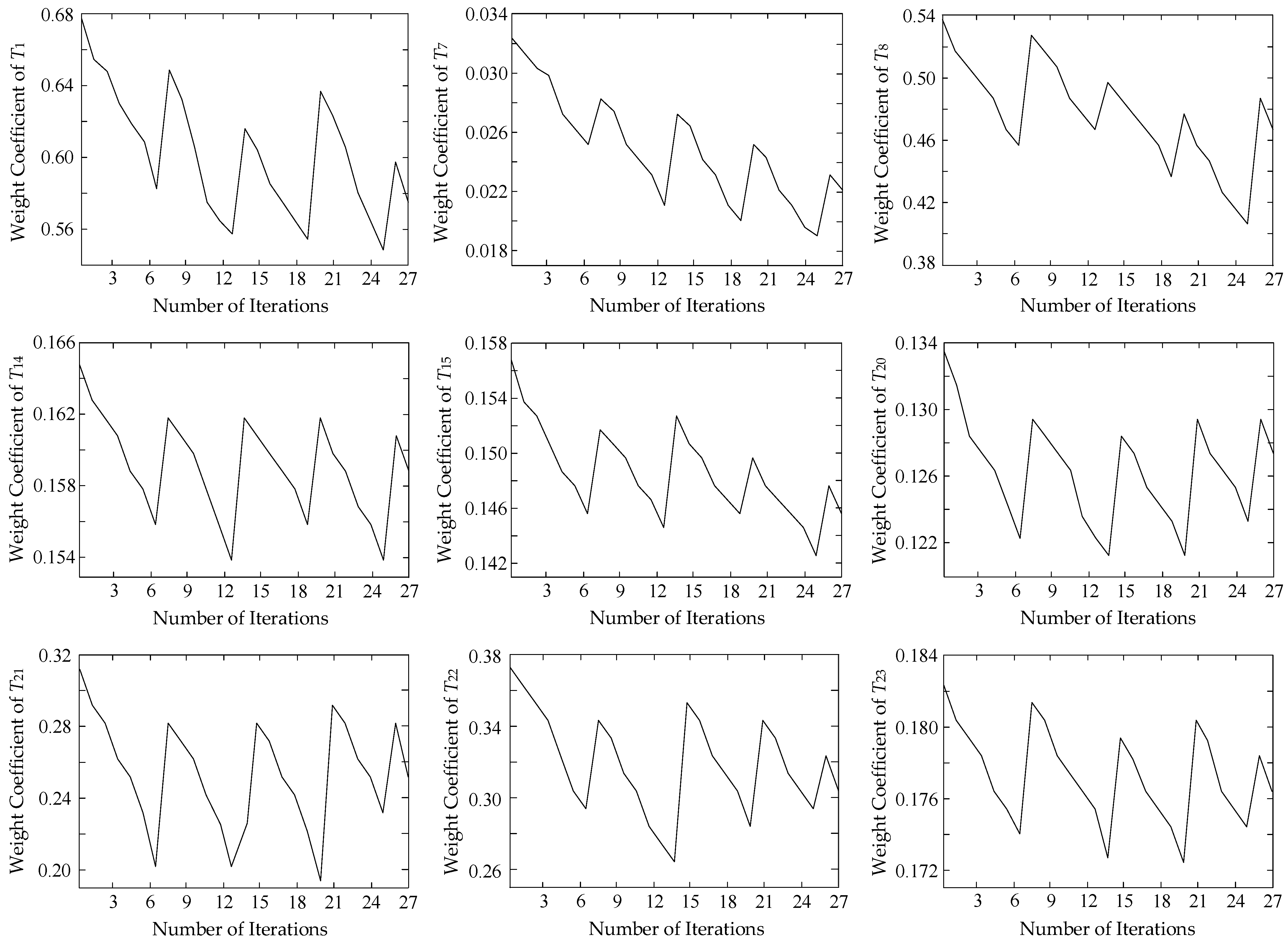
The improved ReliefF is used to calculate the feature weights of the remaining feature sets. Use the typical cross-validation theory to unify the training set and test set of each fault aerial mode current. The results of the feature optimal subset weight calculation are shown in Appendix A.

According to the data in Appendix A, take the average of the 27 calculation results of the weight of 9 kinds of features, and obtain the weight value as shown in

Table 3. Weight coefficient of the optimal features.

Optimal Features Tp	Weight Coefficient W(Tp)	Optimal Features Tp	Weight Coefficient W(Tp)
T1	0.621978	T20	0.126173
T7	0.029730	T21	0.258922
T8	0.592293	T22	0.321860
T14	0.147733	T23	0.177813
T15	0.131527	-	-

.

For the RF regression model, the fitting superiority of the model can be judged by R². The calculation formula of R² is:

$$R^2=1-\frac{{\displaystyle \sum _{i=1}^n{(y_i-{\hat{y}}_i)}^2}}{{\displaystyle \sum _{i=1}^n{(y_i-\overline{y})}^2}}$$

(9)

Use loop statements while building the RF model to find the optimal parameter that maximizes R². From the results of the multiple loops, R² was taken to the maximum value of 98.88 when mtry = 4 and ntree = 500. The traditional RF and improved WRF are used as fitters to evaluate the feature selection results. The corresponding OOB error rates are shown in Figure 7. After improving the feature preprocessing of the ReliefF algorithm, when the number of decision trees is large, the OOB error can be maintained at a low level of around 2.2%. However, the performance of this algorithm cannot meet some higher requirements and needs to be further processed.

As shown in Figure 7, after using the WRF to replace the traditional RF as the estimator, the accuracy and performance of the model are greatly improved. The OOB error can reach about 0.4%, the corresponding ntree when the iteration convergence is reduced, and the convergence speed is improved.

After establishing the fault location model, the cross-validation theory is cyclically used for simulation verification. Randomly assume 19 fault locations f_n (n = 1, 2, …, 19) on Line 1, and the results are shown in

Table 4. Fault location results and errors.

x(actual)/km	Random Forest		Weighted Random Forest
	x(measure)/km	Perror/%	x(measure)/km	Perror/%
0.3	0.2301	0.699	0.2957	0.043
0.8	0.8036	0.036	0.8027	0.027
1.0	1.0077	0.077	1.0055	0.055
1.5	1.5224	0.224	1.5030	0.030
2.0	2.0139	0.139	2.0017	0.017
2.7	2.7427	0.427	2.7029	0.029
3.0	3.0350	0.350	3.0084	0.084
3.1	3.1227	0.227	3.1027	0.027
4.0	4.0383	0.383	4.0073	0.073
4.4	4.4523	0.523	4.4083	0.083
5.0	5.0339	0.339	5.0009	0.009
5.6	5.5220	0.780	5.6014	0.014
6.0	6.0921	0.921	6.0113	0.113
7.0	7.0801	0.801	7.0101	0.101
7.3	7.3007	0.007	7.3007	0.007
8.0	8.0088	0.088	8.0068	0.068
8.8	8.8311	0.311	8.8086	0.086
9.0	9.0628	0.628	9.0091	0.091
9.8	9.8825	0.825	9.8095	0.095

. The formula of the absolute value of the locating error percentage P_error is:

$$P_{\mathit{error}}=\left|\frac{x_{\left(\mathit{measure}\right)}-x_{\left(\mathit{actual}\right)}}{L_{\mathit{line}}}\right|\times 100\%$$

(10)

where x_(measure) and x_(actual) are the distance between the fault location calculated by the algorithm and the actual fault location from bus A, respectively. L_line is the length of the DC line.

It can be seen from Table 4 that the fault location method of the DC distribution network proposed in this paper has a high accuracy. The absolute value of the error rate can basically be maintained below 0.1%, and the average value has dropped about 10 times to 0.055%.

Due to the randomness of intelligent algorithm fitting, the results of each simulation verification may be slightly different, but they can meet the requirements of accuracy and rapidity in general. Only when the parameters or the topology of the system change, does the algorithm model need to be re-established for the system. Under normal circumstances, we extract the aerial mode current of port A and input the constructed model to complete the monopolar grounding fault location of the system.

5.2. Effect of Fault Resistances

When the monopolar grounding fault occurs in the actual DC distribution network, the fault resistance is generally small. The maximum value of fault resistance does not exceed 100 Ω. In order to reflect the general validity of the algorithm, this paper simulates the monopolar grounding fault under R_f = 10 Ω and R_f = 100 Ω on the basis of Section 5.1.

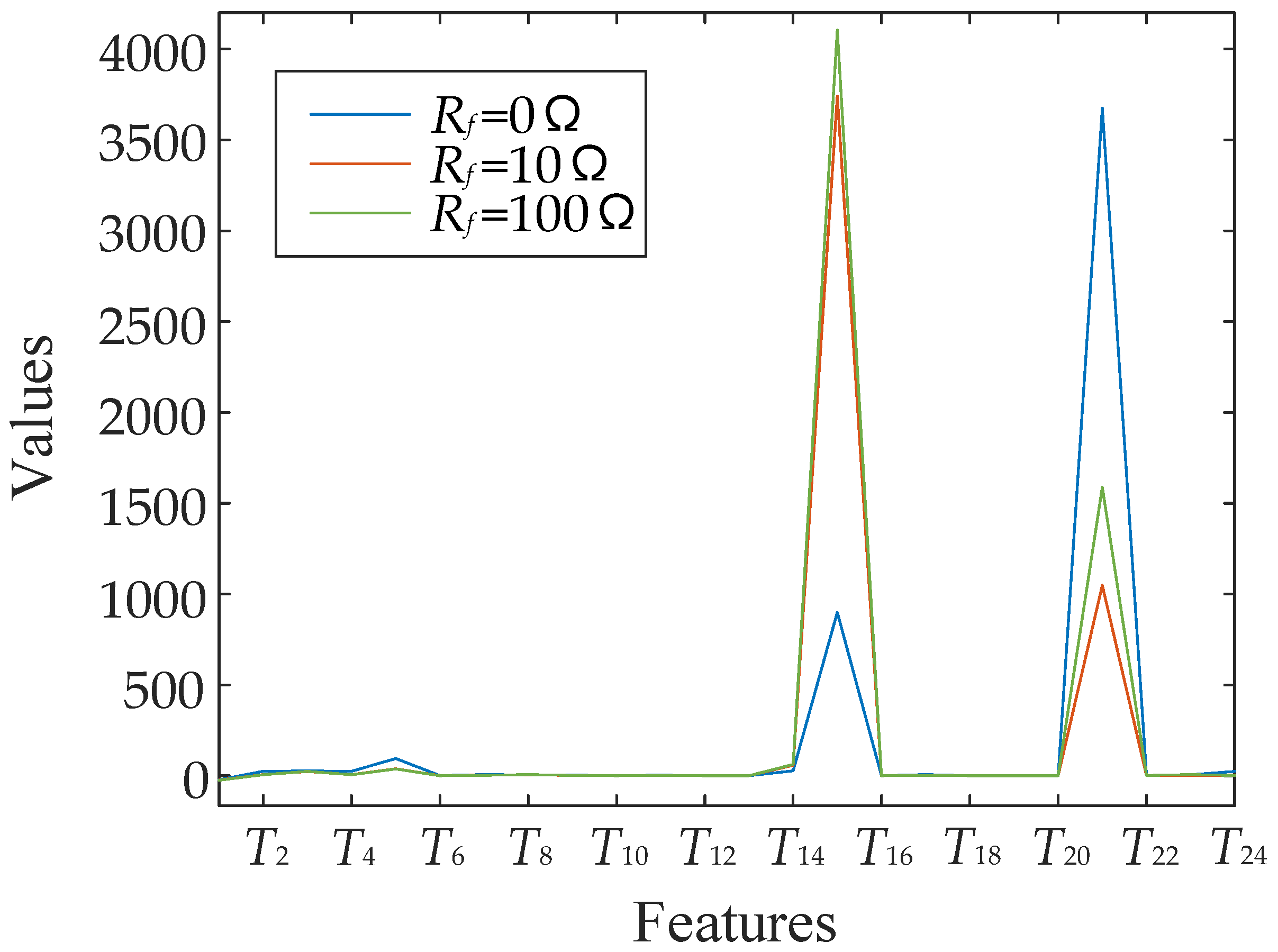
There are large quantities of fault current data under different fault resistances, which is difficult to be shown in total. Here, taking the fault of Line 1 at a distance of 5 km from the head of the line (midpoint of the line) as an example, the fault current and corresponding fault characteristics are shown with different fault resistance.

As can be seen from Figure 8, when the fault resistance increases, the amplitude of the aerial mode current will decrease, and the hazard will be reduced. However, the difficulty of fault location increases, and the conventional fault location method may cause the failure of the location accuracy to meet the requirements.

The 24 fault features and values under different fault resistances are shown in

Table 5. Fault features and values with fault resistance.

Fault Resistances	Fault Features and Values
Rf = 0 Ω	T1	T2	T3	T4	T5	T6	T7	T8
	−22.4555345	24.5180054	26.4290631	24.5192314	95.1385402	1.11573634	6.26347973	3.88015997
	T9	T10	T11	T12	T13	T14	T15	T16
	3.59976969	0.84705480	3.28670813	0.03603943	0.34007241	27.6020470	899.678554	0.00167930
	T17	T18	T19	T20	T21	T22	T23	T24
	6.17048228	0.03906557	0.03603943	0.00261003	3674.42539	2.13959375	5.89237887	24.1578590
Rf = 10 Ω	T1	T2	T3	T4	T5	T6	T7	T8
	−23.7409934	6.69391958	23.1461072	6.69425430	38.1291214	0.71045427	3.42611937	5.69579817
	T9	T10	T11	T12	T13	T14	T15	T16
	1.64732329	0.28197027	1.60604574	0.01798488	0.13035299	57.9065772	3739.96752	0.00208018
	T17	T18	T19	T20	T21	T22	T23	T24
	2.18045779	0.01394780	0.01798488	0.00584912	1048.20842	0.90658752	1.21975124	3.91253691
Rf = 100 Ω	T1	T2	T3	T4	T5	T6	T7	T8
	−24.4414665	5.61344182	24.0988859	5.61372252	37.5885683	0.12268724	2.56588102	6.69583653
	T9	T10	T11	T12	T13	T14	T15	T16
	1.55976373	0.22968027	1.53790151	0.01211139	0.13196106	61.8340625	4103.87198	0.00093823
	T17	T18	T19	T20	T21	T22	T23	T24
	1.49022602	0.00947254	0.01211139	0.00256927	1588.33645	1.98663941	6.17647147	2.00997774

, and as can be seen from Figure 8, when the fault resistance increases, the amplitude of the aerial mode current will decrease, and the hazard will be reduced. However, the difficulty of fault location increases, and the conventional fault location method may cause the failure of the location accuracy to meet the requirements.

The 24 fault features and values under different fault resistances are shown in Table 5 and Figure 9.

After the features selection and weight calculation, the features and weights are input into the WRF model for fault location estimation. The simulation results are shown in Figure 10 and Appendix B 

Table A1. Fault location results and errors with transition resistors.

x(actual)/km	Rf = 10 Ω		Rf = 100 Ω
	x(measure)/km	Perror/%	x(measure)/km	Perror/%
0.3	0.2870	0.130	0.2672	0.328
0.8	0.7997	0.003	0.7894	0.106
1.0	1.0320	0.320	1.0425	0.425
1.5	1.5009	0.009	1.5107	0.107
2.0	1.9963	0.037	1.9866	0.134
2.7	2.7222	0.222	2.7528	0.528
3.0	3.0323	0.323	3.0423	0.423
3.1	3.1043	0.043	3.1140	0.140
4.0	4.0072	0.072	4.0179	0.179
4.4	4.4024	0.024	4.4121	0.121
5.0	5.0097	0.097	5.0192	0.192
5.6	5.6299	0.299	5.6390	0.390
6.0	6.0390	0.390	6.0491	0.491
7.0	7.0014	0.014	7.0417	0.417
7.3	7.3001	0.001	7.3105	0.105
8.0	8.0029	0.029	8.0126	0.126
8.8	8.8189	0.189	8.8284	0.284
9.0	8.9877	0.123	8.9778	0.222
9.8	9.8318	0.318	9.8319	0.319

.

It is obvious that the transition resistance has little effect on the fault location accuracy, which is determined by the properties of the algorithm itself. Even if the fault resistance is 100 Ω, the locating error rate of the proposed method can still be kept within 0.85%, and the absolute value of the maximum positioning error rate is 0.8100%, which corresponds to only 0.081 km on a 10 km distribution line. It shows that the fault location method proposed in this paper has a certain ability to resist fault resistances and has strong robustness.

5.3. Effect of Noise

In order to test the anti-noise ability of the method proposed in this paper, Gaussian white noise with signal-to-noise ratios of 60 dB, 40 dB and 20 dB is added to the monopolar grounding fault model. The simulation results are shown in Figure 11 and Appendix B 

Table A2. Fault location results and errors with white noise.

x(actual)/km	SNR = 60 dB		SNR = 40 dB		SNR = 20 dB
	x(measure)/km	Perror/%	x(measure)/km	Perror/%	x(measure)/km	Perror/%
0.3	0.2670	0.330	0.2660	0.340	0.2654	0.346
0.8	0.7790	0.210	0.7784	0.216	0.7777	0.223
1.0	1.0354	0.354	1.0427	0.427	1.0508	0.508
1.5	1.5093	0.093	1.5170	0.170	1.5245	0.245
2.0	1.9878	0.122	1.9875	0.125	1.9876	0.124
2.7	2.7273	0.273	2.7317	0.317	2.7363	0.363
3.0	3.0256	0.256	3.0251	0.251	3.0241	0.241
3.1	3.1220	0.220	3.1250	0.250	3.1282	0.282
4.0	4.0041	0.041	4.0042	0.042	4.0034	0.034
4.4	4.4089	0.089	4.4171	0.171	4.4253	0.253
5.0	5.0096	0.096	5.0143	0.143	5.0195	0.195
5.6	5.6202	0.202	5.6307	0.307	5.6414	0.414
6.0	6.0291	0.291	6.0338	0.338	6.0386	0.386
7.0	7.0163	0.163	7.0174	0.174	7.0187	0.187
7.3	7.3121	0.121	7.3262	0.262	7.3400	0.400
8.0	8.0059	0.059	8.0151	0.151	8.0243	0.243
8.8	8.8148	0.148	8.8283	0.283	8.8411	0.411
9.0	8.9876	0.124	8.9727	0.273	8.9572	0.428
9.8	9.8302	0.302	9.8471	0.471	9.8638	0.638

.

It can be seen that the fault location method has a strong anti-noise ability. In the case of strong noise interference in the collected aerial mode current, it still has an excellent fault location capability.

5.4. Effect of Time Window Length

Compared with the pole-to-pole short-circuit of the DC line, the monopolar grounding does not have an impulse current, which provides the possibility to obtain fault information within a relatively long time window after the fault. Although the training of the model takes a certain amount of time, once the model is finished, the transient aerial mode current signal can be propagated and calculated to obtain the fault location within milliseconds. The method proposed in this paper can quickly achieve fault location.

In the proposed method, the complete period DFT is applied within the 100 ms time window of the fault aerial mode current. At a constant sampling frequency, the longer the data time window, the greater the frequency resolution and harmonic content and vice versa. All stages of algorithm construction and testing are repeated in a DC distribution system by setting different time window lengths. Figure 12 and Appendix B 

Table A3. Fault location results and errors with data window length.

x(actual)/km	80 ms Data Window Length		50 ms Data Window Length
	x(measure)/km	Perror/%	x(measure)/km	Perror/%
0.3	0.2741	0.259	0.2619	0.381
0.8	0.8673	0.673	0.8565	0.565
1.0	1.0455	0.455	1.0651	0.651
1.5	1.5789	0.789	1.5885	0.885
2.0	2.0407	0.407	2.0512	0.512
2.7	2.6699	0.301	2.6582	0.418
3.0	3.0409	0.409	3.0518	0.518
3.1	3.1014	0.014	3.1118	0.118
4.0	4.0103	0.103	4.0211	0.211
4.4	4.4116	0.116	4.4270	0.270
5.0	5.0476	0.476	5.0567	0.567
5.6	5.5516	0.484	5.6416	0.416
6.0	6.0141	0.141	6.0214	0.214
7.0	7.0761	0.761	7.0828	0.828
7.3	7.3052	0.052	7.3158	0.158
8.0	8.0052	0.052	8.0195	0.195
8.8	8.8271	0.271	8.8399	0.399
9.0	9.0712	0.712	9.0801	0.845
9.8	9.8473	0.473	9.8586	0.457

show the average fault location error rate for the test set with different time windows.

It can be seen from Figure 12 that changing the length of the time window has a certain impact on the accuracy of the fault location method, but the overall location deviation remains within the allowable range. This means that the accuracy of the improved WRF model no longer depends too much on the size of the sample data but more on the optimal features selected by pre-processing. Considering the cost and the actual requirements for location accuracy, the method proposed in this paper can shorten the data window to between 50 ms and 80 ms depending on the specific situation.

5.5. Comparison with Other Estimators and Intelligent Fault Location Methods

The WRF estimator is utilized in this fault location method. To compare and illustrate the superiority of the WRF estimator, the same fault location experiments were performed in the six-terminal DC distribution system of Figure 1 using the MLPNN and ε-SVR estimators. The proper structure of each MLPNN estimator was determined through a trial-and-error process. The best parameters values for the ε-SVR estimator were selected through a 10-fold cross-validation procedure.

The results of MLPNN, ε-SVR, RF and WRF estimators applied to fault location are shown in

Table 6. Comparison with other estimators.

Estimators	Positive Pole-to-Ground	Negative Pole-to-Ground
	Perror/%	Perror/%
MLPNN	0.2093	0.2188
Ε-SVR	0.8280	0.0791
RF	0.4097	0.4311
WRF	0.0554	0.0592

.

As shown in Table 6, the location accuracy of WRF is higher than the other three estimators. The accuracy of the MLPNN estimator in fault location is acceptable compared to the ε-SVR. However, the WRF estimator has easier parameter selection and better overall test performance when dealing with high-dimensional input feature vectors.

The weighted random forest algorithm proposed in this paper belongs to the category of machine-learning-based fault location methods. Therefore,

Table 7. Comparison with other intelligent fault location methods.

Fault Location Method	Required Current Data	Sampling Frequency	Perror/%
continuous wavelet transform and Pearson correlation coefficient based on pattern matching [22]	current data for multiple points across the line	5 kHz	0.2079
current frequency spectra based on MLPNN method [23]	two-terminal current data of the line	10 kHz	0.5370
Hilbert–Huang transform and bat algorithm based on SVR method [24]	one-terminal current data of the line	1000 kHz	0.3104
Improved ReliefF and WRF fault location method in this paper	one-terminal current data of the line	100 kHz	0.0554

compares the performance of this method with the existing intelligent fault location methods.

As can be seen from Table 7, the method proposed in this paper requires less information, lower sampling frequency, and has higher accuracy compared to other intelligent fault location methods. Although the method proposed in the literature [22] has high accuracy and requires lower sampling frequency, it requires many current sensors to be installed along the DC line to collect current data from multiple points, which may increase the complexity and cost. The method in the literature [23] requires the current data at both terminals of the line and has insufficient location accuracy. The method in the literature [24] requires a very high sampling frequency, and if the sampling rate is reduced to 250 kHz, its P_error may increase by about 12 times. This requirement would significantly increase the cost and reduce the practicality of fault location.

5.6. Application to Fault Line Identification

The fault location method proposed in this paper is realized by constructing a fault location model through a machine learning technique and fitting the specific fault location. This idea can also be applied to the identification of fault line in asymmetric ring DC distribution networks.

The cross-validation method was also used to set positive pole-to-ground short-circuit at multiple positions in Line 1~Line 6 in Figure 1. The method proposed in this paper was used to construct the improved ReliefF and WRF algorithm for simulation verification. The results show that the identification accuracy can reach 100%. That is to say, the method proposed in this paper can also be used to identify the fault line of the DC ring network. However, it should be noted that there may be problems such as a dead band near the bus of the DC line, and it is not suitable for a symmetrical ring network. It is necessary to combine other fault criteria to realize the fault line of the ring DC distribution system with high accuracy.

6. Conclusions

This paper proposes a fault location method based on improved ReliefF and weighted random forest. Combined with multiple time and frequency-domain features, the fault location of the DC distribution network was estimated. A six-terminal ring DC distribution system was established for simulation verification, considering various factors affecting the positioning results and comparing with existing works in many aspects. The result shows that the method proposed in this paper has high accuracy under various conditions, and the average error is within 0.1%. It has strong anti-transition resistance and anti-noise ability within a certain time window, and has strong adaptability. The method is simple in principle, only needs to be measured locally, and does not need to synchronize the information at both terminals, which greatly reduces the management and investment costs of sampling equipment. In view of the above advantages, the method proposed in this paper is beneficial to the reliable and stable operation of the DC distribution network and has certain engineering practicability.

References

- Han, B.; Li, Y. Simulation Test of a DC Fault Current Limiter for Fault Ride-Through Problem of Low-Voltage DC Distribution. Energies 2020, 13, 1753. [Google Scholar] [CrossRef] [Green Version]
- Cai, H.; Yuan, X.; Xiong, W.; Zheng, H.; Xu, Y.; Cai, Y.; Zhong, J. Flexible Interconnected Distribution Network with Embedded DC System and Its Dynamic Reconfiguration. Energies 2022, 15, 5589. [Google Scholar] [CrossRef]
- Jia, K.; Xuan, Z.; Feng, T.; Wang, C.; Bi, T.; Thomas, D.W.P. Transient High-Frequency Impedance Comparison-Based Protection for Flexible DC Distribution Systems. IEEE Trans. Smart Grid 2020, 11, 323–333. [Google Scholar] [CrossRef]
- Xu, Y.; Liu, J.; Jin, W.; Fu, Y.; Yang, H. Fault Location Method for DC Distribution Systems Based on Parameter Identification. Energies 2018, 11, 1983. [Google Scholar] [CrossRef] [Green Version]
- Li, M.; Jia, K.; Bi, T.; Yang, Q. Sixth harmonic-based fault location for VSC-DC distribution systems. IET Gener. Transm. Distrib. 2017, 11, 3485–3490. [Google Scholar] [CrossRef]
- Wang, S.; Fan, C.; Jiang, S. Fault protection scheme for DC distribution network based on ratio of transient voltage principle. Electr. Power Autom. Equip. 2020, 40, 196–205. [Google Scholar]
- Wang, X.; Gao, J.; Wu, L.; Song, G.; Wei, Y. A high impedance fault detection method for flexible DC distribution network. Trans. China Electrotech. Soc. 2019, 34, 2806–2819. [Google Scholar]
- Wang, C.; Jia, K.; Bi, T.; Xuan, Z.; Zhu, R. Transient current curvature based protection for multi-terminal flexible DC distribution systems. IET Gener. Transm. Distrib. 2019, 13, 3484–3492. [Google Scholar] [CrossRef]
- Wu, Y.; Ye, Y.; Ma, X.; Li, Z.; Wu, T.; Xu, H. Single pole-to-ground fault locating method with ability against synchronization error and high fault resistance for DC distribution network. Electr. Power Autom. Equip. 2022, 42, 1–8. [Google Scholar]
- Masaoki, A.; Schweitzer, E.; Baker, R. Development and field-data evaluation of single-end fault locator for two-terminal HVDC transmission lines-II:algorithm and evaluation. IEEE Trans. Power Appar. Syst. 1985, 104, 3531–3537. [Google Scholar]
- Cheng, J.; Guan, M.; Tang, L.; Huang, H.; Chen, X.; Xie, J. Paralleled multi-terminal DC transmission line fault locating method based on travelling wave. IET Gener. Transm. Distrib. 2014, 8, 2092–2101. [Google Scholar] [CrossRef]
- He, Z.; Liao, K.; Li, X.; Lin, S.; Yang, J.; Mai, R. Natural frequency-based Line fault location in HVDC Lines. IEEE Trans. Power Deliv. 2014, 29, 851–859. [Google Scholar] [CrossRef]
- Zhang, S.; Zou, G.; Huang, Q.; Gao, H. A traveling-wave-based fault location scheme for MMC-based multi-terminal DC grids. Energies 2018, 11, 401. [Google Scholar] [CrossRef] [Green Version]
- Xu, Y.; Liu, J.; Zhang, S. Fault Location Method Based on Genetic Algorithm for DC Distribution Network. Acta Energ. Sol. Sin. 2020, 41, 1–8. [Google Scholar]
- Ma, C.; Li, B.; He, J.; Li, Y.; Mao, Q.; Wang, S.; Li, G.; Hu, Z. The improved fault location method for flexible direct current grid based on clustering and iterating algorithm. IET Renew. Power Gener. 2021, 15, 3577–3587. [Google Scholar] [CrossRef]
- Yang, H.; Xu, Y.; Qin, B.; Wang, Q. Fault Location Method for DC Distribution Network Based on Particle Swarm Optimization. In Proceedings of the2019 IEEE 2nd International Conference on Electronics Technology (ICET), Chengdu, China, 10–13 May 2019. [Google Scholar]
- Mohammad, F. Locating Short-circuit Faults in HVDC Systems Using Automatically Selected Frequency-domain Features. Int. Trans. Trans. Electr. Energy Syst. 2019, 29, e2765. [Google Scholar]
- Su, W.; Yang, J.; Jia, Y.; Xiao, X.; Liu, R.; Si, X. Single-terminal traveling wave line selection in DC distribution system. In Proceedings of the 16th IET International Conference on AC and DC Power Transmission (ACDC 2020), Online Conference, 2–3 July 2020. [Google Scholar]
- Saber, A.; Zeineldin, H.H.; El-Fouly, T.H.M.; Al-Durra, A. Time-Domain Fault Location Algorithm for Double-Circuit Transmission Lines Connected to Large Scale Wind Farms. IEEE Access 2021, 9, 11393–11404. [Google Scholar] [CrossRef]
- Yang, J.; Wang, X.; Wang, D. An Unsupervised Feature Selection Method Based on Improved ReliefF and Bisecting K-means. In Proceedings of the International Conference on Network Infrastructure and Digital Content (IC-NIDC), Guiyang, China, 22–24 August 2018. [Google Scholar]
- Peker, M.; Arslan, A.; Şen, B.; Çelebi, F.V.; But, A. A novel hybrid method for determining the depth of anesthesia level: Combining ReliefF feature selection and random forest algorithm (ReliefF+RF). In Proceedings of the International Symposium on Innovations in Intelligent SysTems and Applications (INISTA), Madrid, Spain, 2–4 September 2015. [Google Scholar]
- Tzelepis, D.; Dyśko, A.; Fusiek, G.; Niewczas, P.; Mirsaeidi, S.; Booth, C.; Dong, X. Advanced fault location in MTDC networks utilising optically-multiplexed current measurements and machine learning approach. Int. J. Electr. Power Energy Syst. 2018, 97, 319–333. [Google Scholar] [CrossRef] [Green Version]
- Yang, Q.; Le, B.S.; Aggarwal, R.; Wang, Y.; Li, J. New ANN method for multi-terminal HVDC protection relaying. Electr. Power Syst. Res. 2017, 148 (Suppl. C), 192–201. [Google Scholar] [CrossRef] [Green Version]
- Hao, Y.; Wang, Q.; Li, Y.; Song, W. An intelligent algorithm for fault location on VSC-HVDC system. Int. J. Electr. Power Energy Syst. 2018, 94 (Suppl. C), 116–123. [Google Scholar] [CrossRef]
Figure 1.
Topology of a six-terminal DC distribution network.
Figure 2.
Equivalent circuit for monopolar grounding.
Figure 3.
Aerial mode current for monopolar grounding in different positions.
Figure 4.
Steps of improved ReliefF algorithm.
Figure 5.
Flowchart of the fault location method.
Figure 6.
PCC between features.
Figure 7.
OOB error of random forest algorithm.
Figure 8.
Aerial mode current with fault resistance.
Figure 9.
Fault features and values with fault resistance.
Figure 10.
Fault location results and errors with fault resistors.
Figure 11.
Fault location results and errors with white noise.
Figure 12.
Fault location results and errors with data window length.