
A Hybrid Model for Electricity Demand Forecast Using Improved Ensemble Empirical Mode Decomposition and Recurrent Neural Networks with ERA5 Climate Variables

Abstract
:1. Introduction
2. Materials
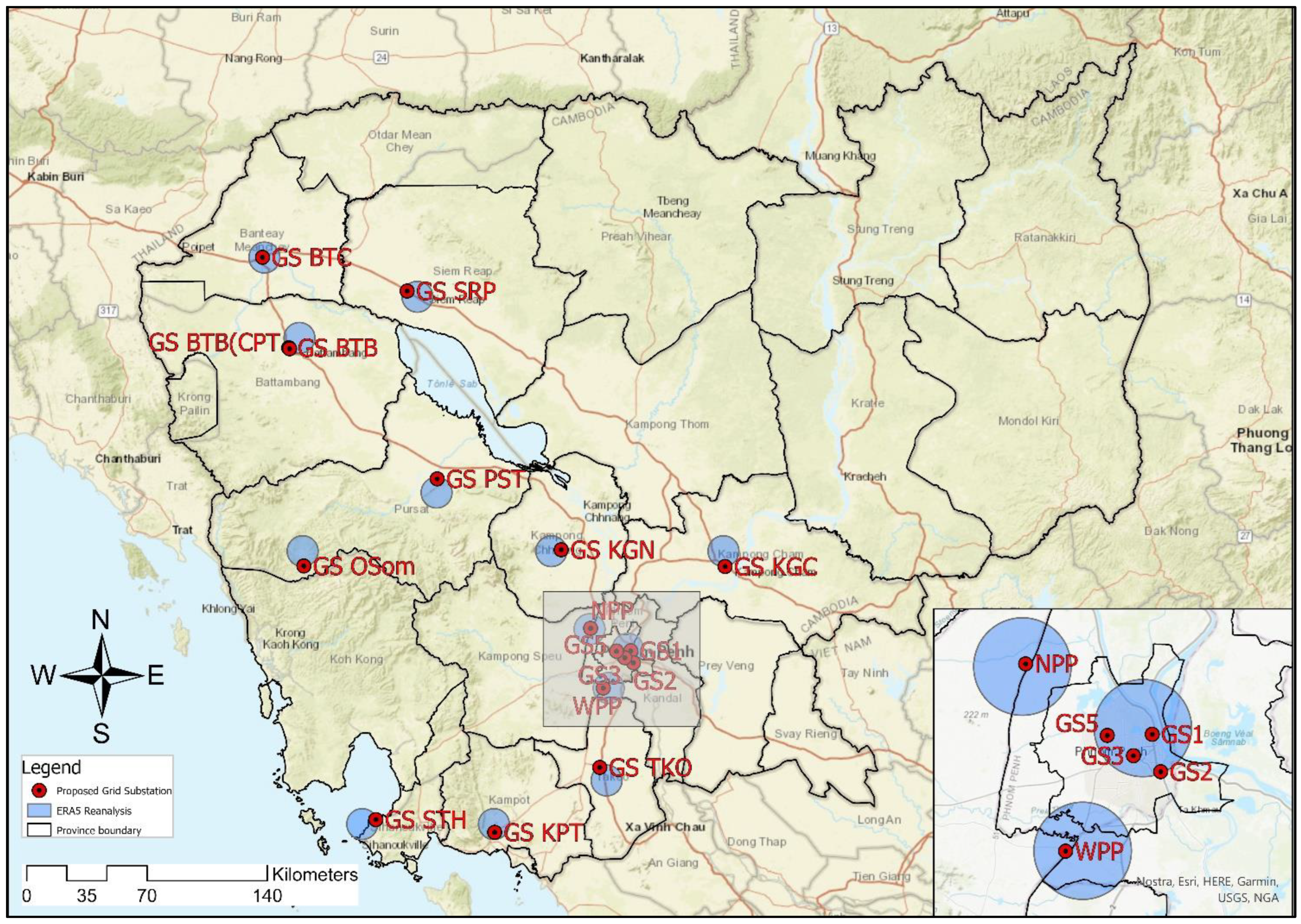
2.1. Study Area
2.2. Data
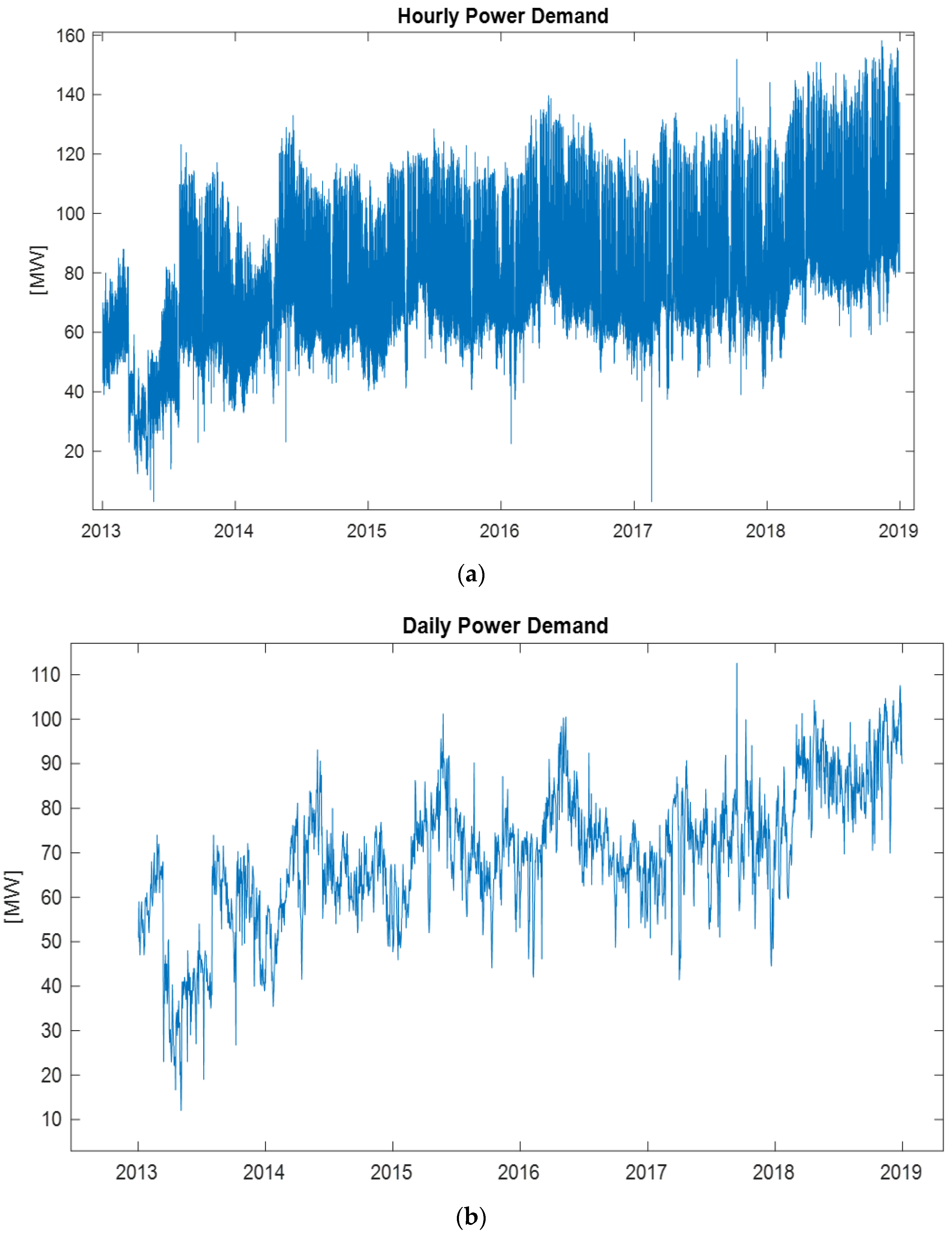
2.2.1. Electricity Demand
2.2.2. ERA5 Climate Reanalysis
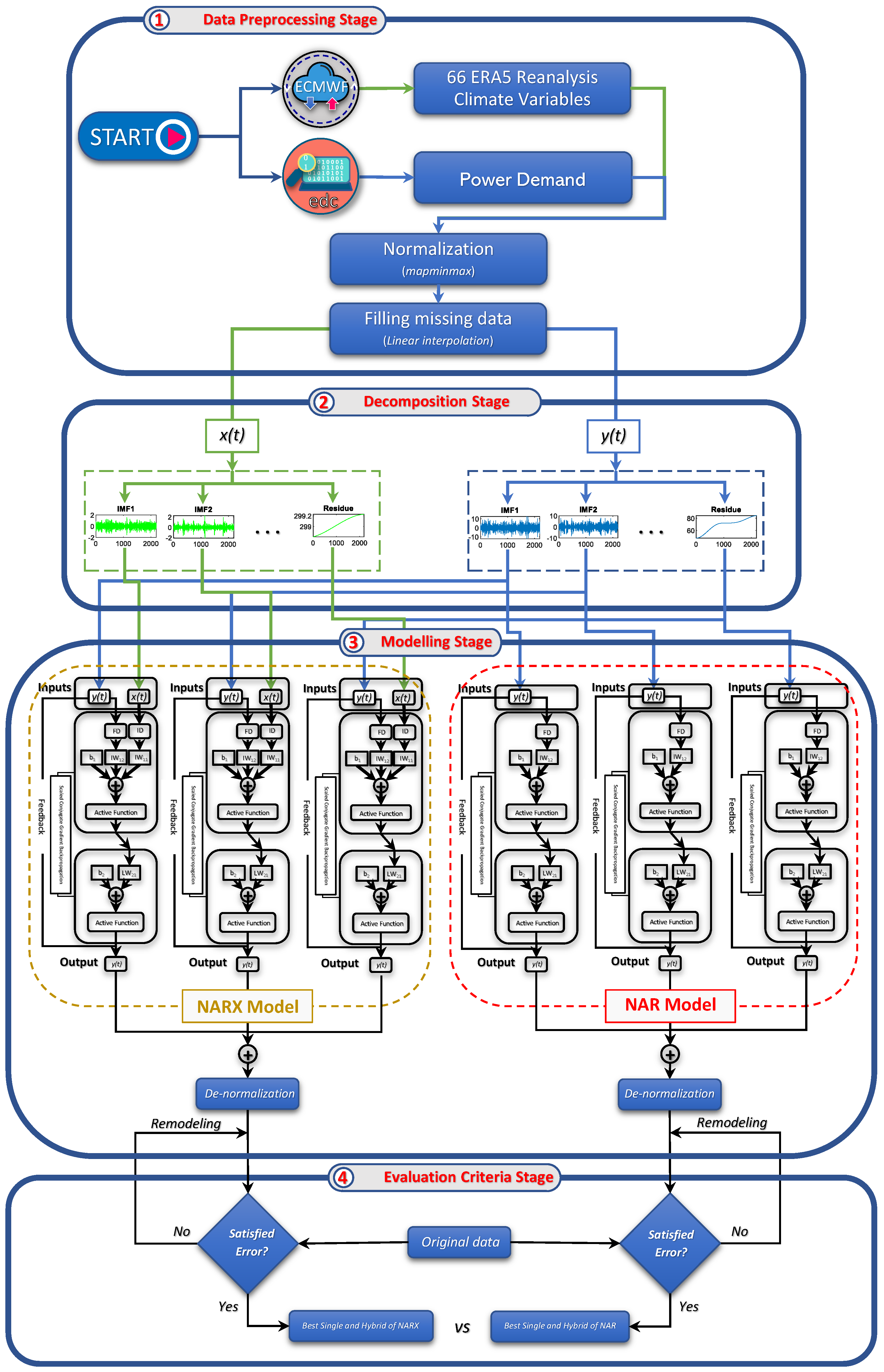
3. Methodology
3.1. Data Preprocessing
3.1.1. Imputation of Missing Values
3.1.2. Normalization of the Input Data
3.2. Decomposition Techniques
3.2.1. Empirical Mode Decomposition (EMD)
3.2.2. Ensemble Empirical Mode Decomposition (EEMD)
3.2.3. Complete EEMD with Adaptive Noise (CEEMDAN)
3.2.4. Improved CEEMDAN
3.3. RNN
3.3.1. NAR Architecture
- (1)
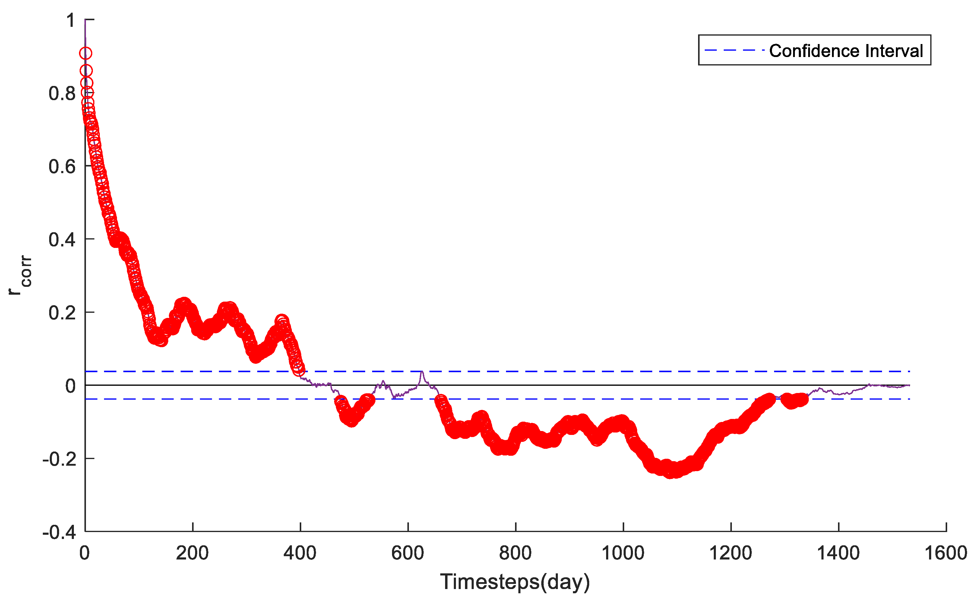
- Feedback delay (FD): The autocorrelation of the training dataset was utilized to identify the FDs, and all significant values were employed as FDs in the model. (Figure 3).
- (2)
- Hidden layers: The number of hidden layer neurons was defined individually each time, for example, 10 neurons [48] and 15 neurons [12], ranging between 3 and 10 [49] and between 1 and 20 [50]. Therefore, the trial-and-error procedure was applied to investigate the number of hidden layer neurons by ranging it from 1 to 20.
- (3)
- Transfer function: Since FDs were utilized in a variety of values, the training time performance is technically the model’s constraint. Therefore, to lessen the need for both memory and time during training, Kumar and Murugan [51] proposed using scaled conjugate gradient-based back-propagation (trainscg) for this model.
- (4)
- Activation function: Sarkar et al. [52] and Vogl et al. [53] stated that the hyperbolic tangent-sigmoidal (tansig) transfer function Equation (18) could provide better results based on an error evaluation during the training process, and this function was accordingly considered as the activation function for the hidden layer and linear function (purelin) (Equation (19)) in the output layer in this study.
- (5)
- Weights and bias: The trial-and-error method employed a double loop for each number of hidden layer neurons, leading to 200 tests with randomly determined beginning weights and biases ranging from 1 to 10.
3.3.2. NARX Architecture
- Step 1.
- Examine the input (climate variables) and target (power demand) from the extracted files, normalize or preprocess these raw data, and convert the data file from an hourly to daily dataset by extracting data at 10:00 a.m. (the peak hour) to represent the daily data.
- Step 2.
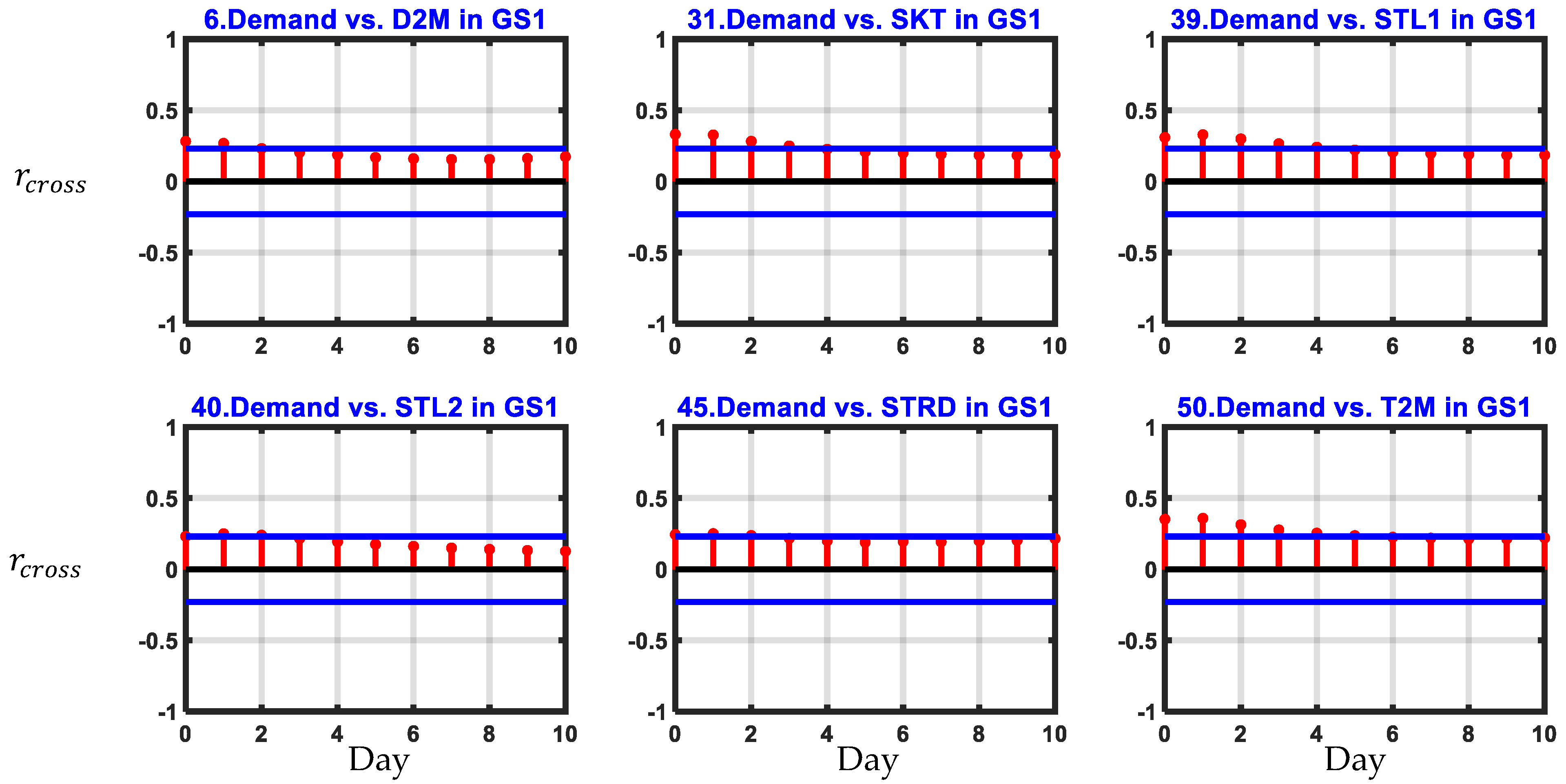
- Define the correlated climate variables using a cross-correlation function between the input (each climate variable) and the target (power demand). Set the bounds for eliminating the variables with low correlations and set the correlation coefficient of lag from 0 to 2 as the ID.
- Step 3.
- For random weight generation, use MAX_TRIAL and MAX_HIDDEN_NEURON to set the maximum number of trials and the maximum number of neurons, respectively, in the hidden layer.
- Step 4.
- Calculate the significant lags using the autocorrelation function and define the number of significant lags as the FD for the network.
- Step 5.
- For the first loop, starting from HIDDEN_NEURON = 1 to MAX_HIDDEN_NEURON = 20.
- Step 6.
- For the second loop, starting from TRIAL = 1 to MAX_TRIAL = 10.
- Step 7.
- Construct an NARX neural network algorithms; specify the input and target vectors, setting up number of hidden layers, training function (trainscg), and the transfer function used in the hidden (tansig) and output (purelin) layers.
- Step 8.
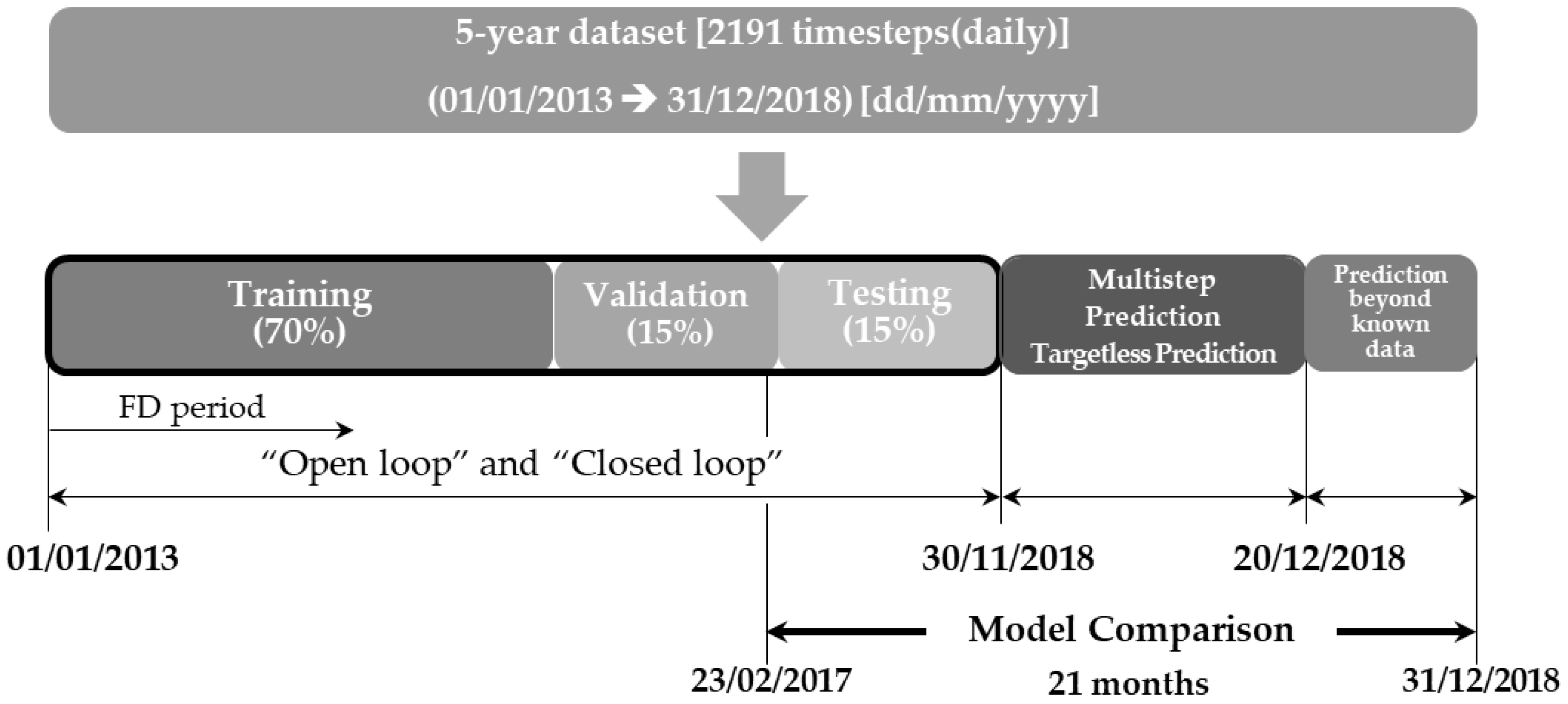
- Divide the dataset in half. First, there is a section for TRAINING, and then, there is a section for MULTISTEP TESTING. In the Section 1, the dataset is divided into training (75 percent), validation (15 percent), and testing (15 percent) datasets using the divideint function. The multistep testing period is utilized to validate the derived prediction in the Section 2.
- Step 9.
- Prepare the data using the preparet function with the input and target of the training period.
- Step 10.
- Train the open-loop neural network using the training function.
- Step 11.
- Simulate the closed-loop neural network using the closeloop function, then use the preparets function to prepare the closed-loop system with closed-loop parameters and execute it with the train function. By using the trained closed-loop network, multistep prediction is simulated with the second part of the dataset.
- Step 12.
- Denormalize or postprocess the simulated output data of the open-loop and closed-loop neural networks. Then, calculate the performance indices of the open-loop (normalized root mean square error (NMSE), , mean absolute error (MAEo), mean absolute percentage error (MAPEo), and root mean square error (RMSEo)), closed-loop (NMSEc, , MAEc, MAPEc, and RMSEc), and multistep prediction networks (NMSEp, , MAEp, MAPEp, and RMSEp).
- Step 13.
- Record the results of the open-loop, closed-loop, and multistep prediction neural networks (the neuron size, number of trials, and performance indices in step 12) if the calculated performance indices are lower than those in the previous iteration. Skip this step otherwise.
- Step 14.
- END\\TRIAL
- Step 15.
- END\\HIDDEN_NEURON
- Step 16.
- From step 13, select the optimum NARX model.
- Step 17.
- Use the optimized NARX model for prediction.
3.4. Hybrid Model
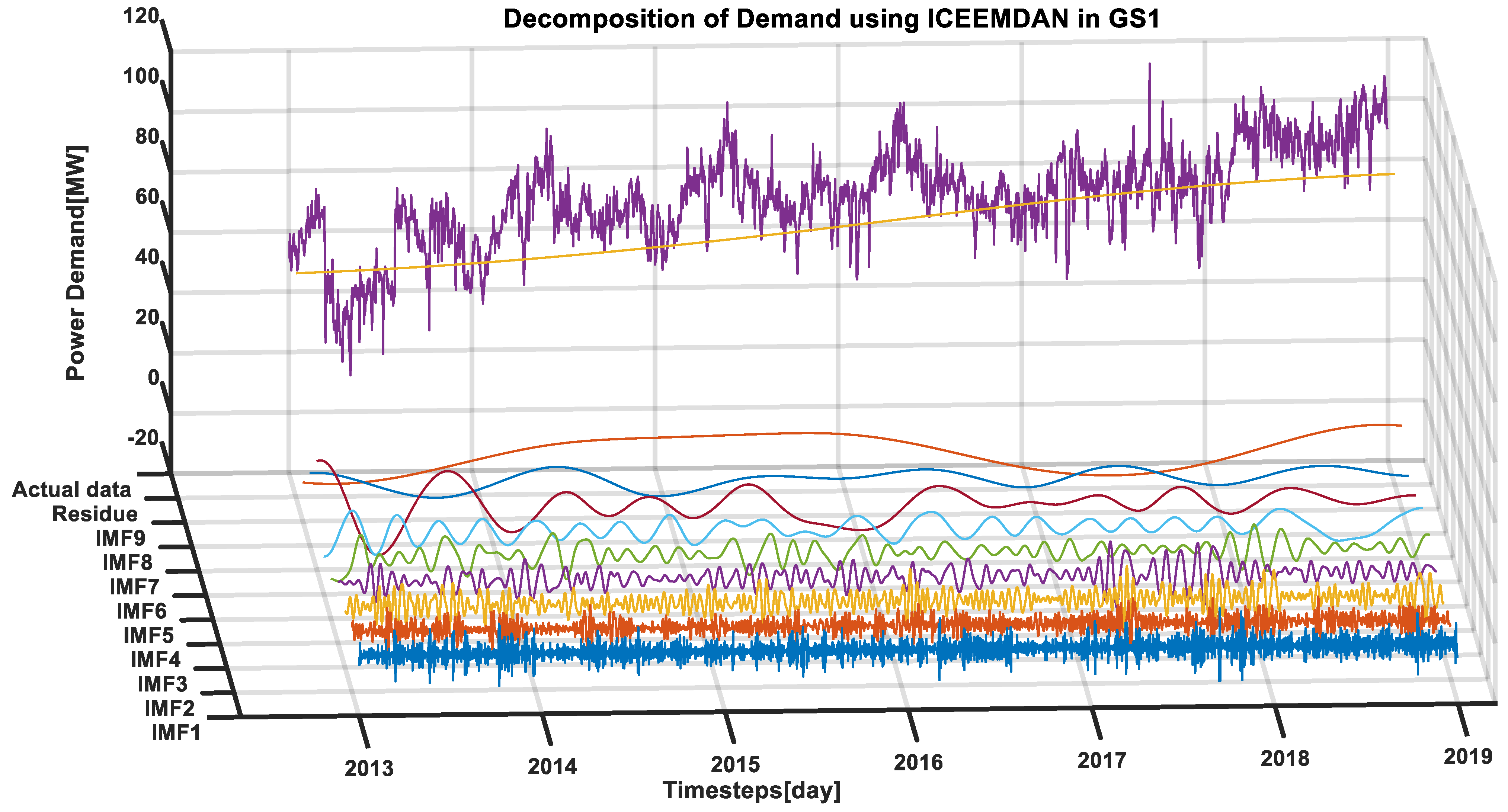
3.4.1. Data Decomposition
3.4.2. Experiments
3.5. Performance Evaluation
4. Results
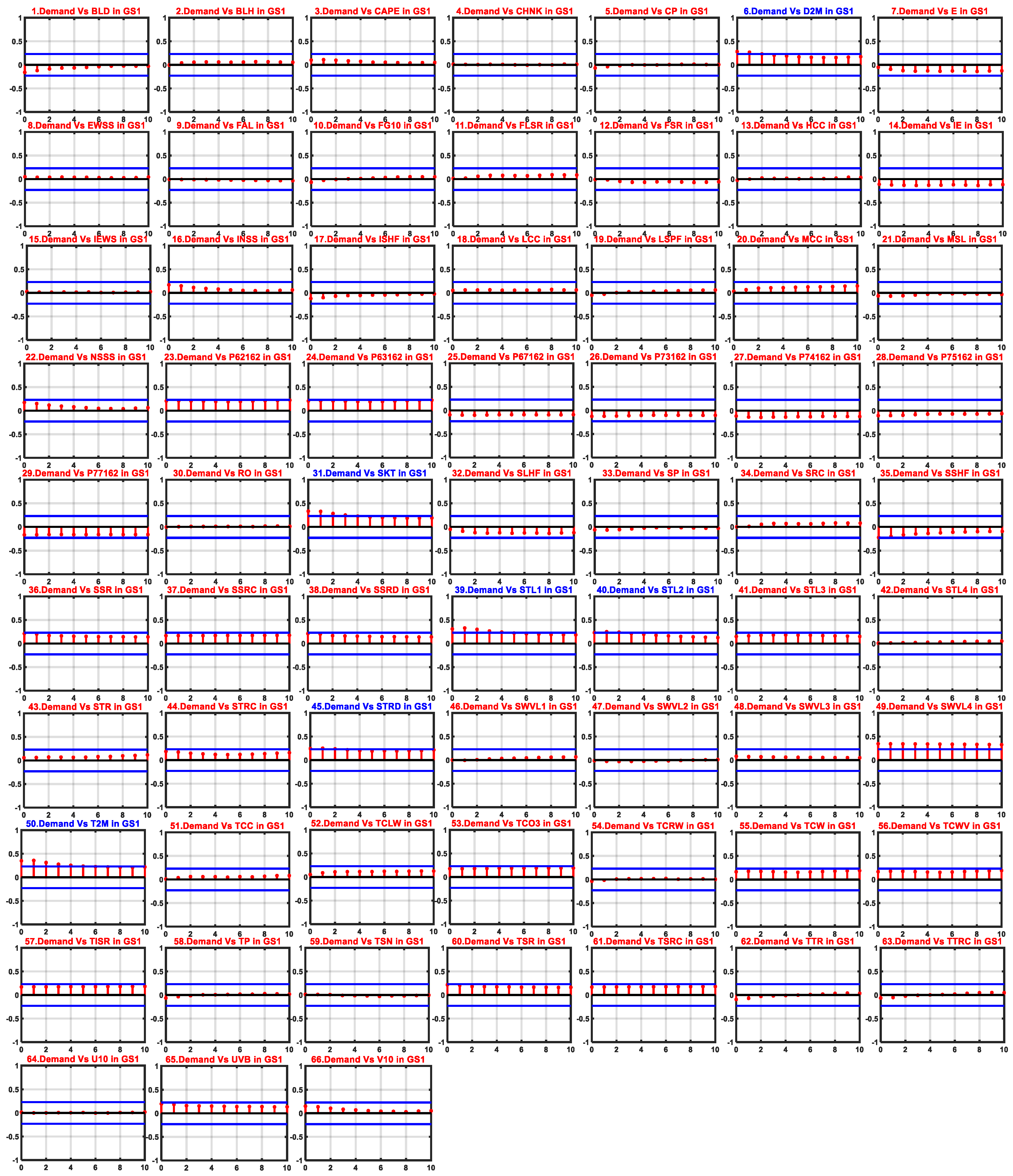
4.1. Climate Variables
4.2. Decomposition Result
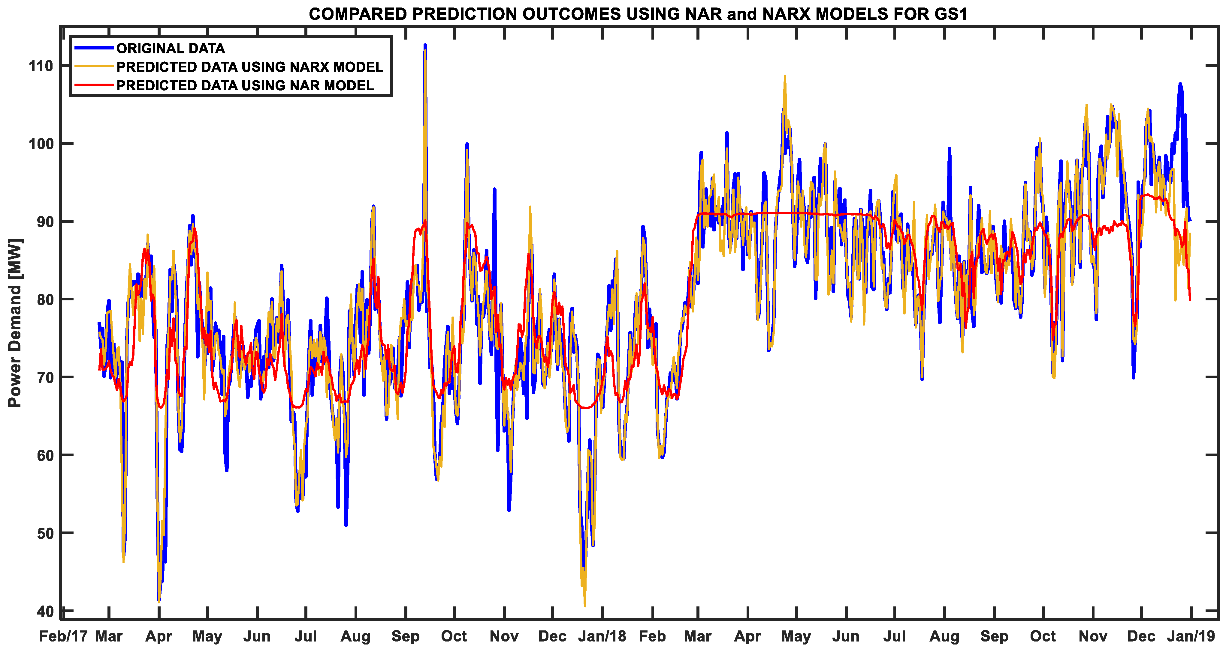
4.3. Stand-Alone Models
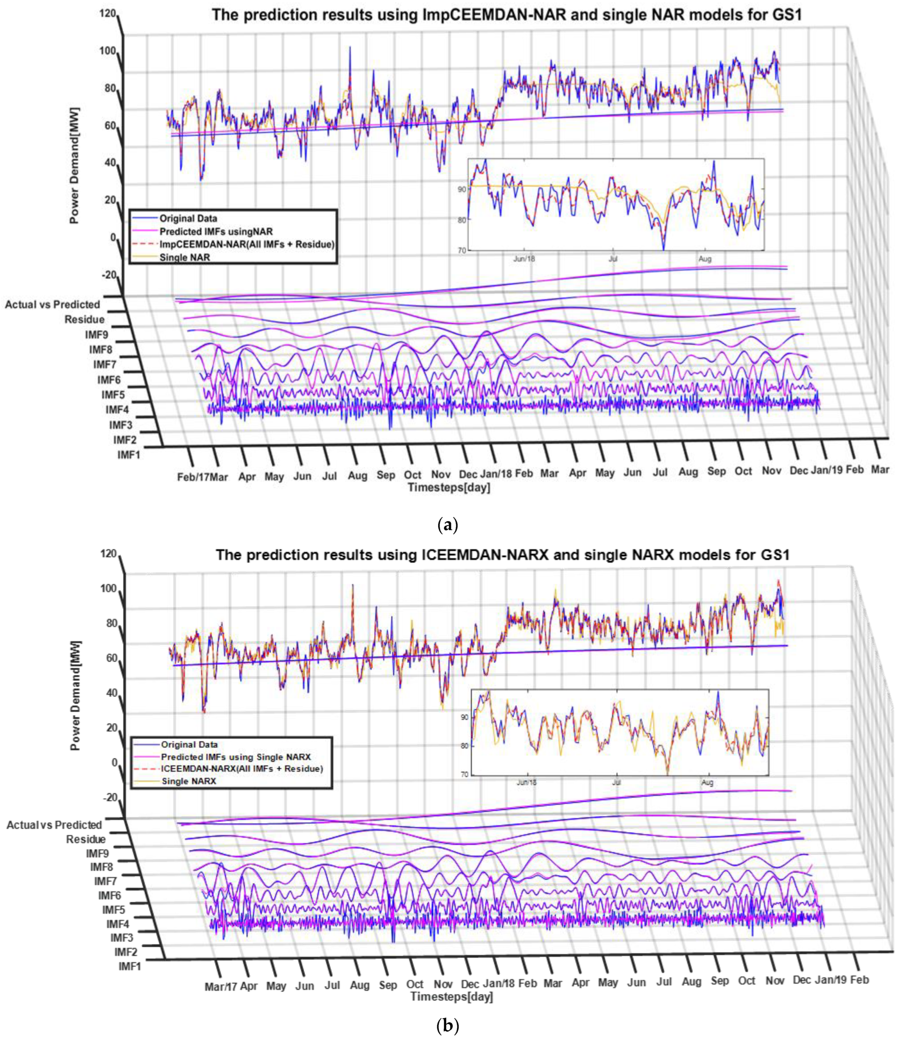
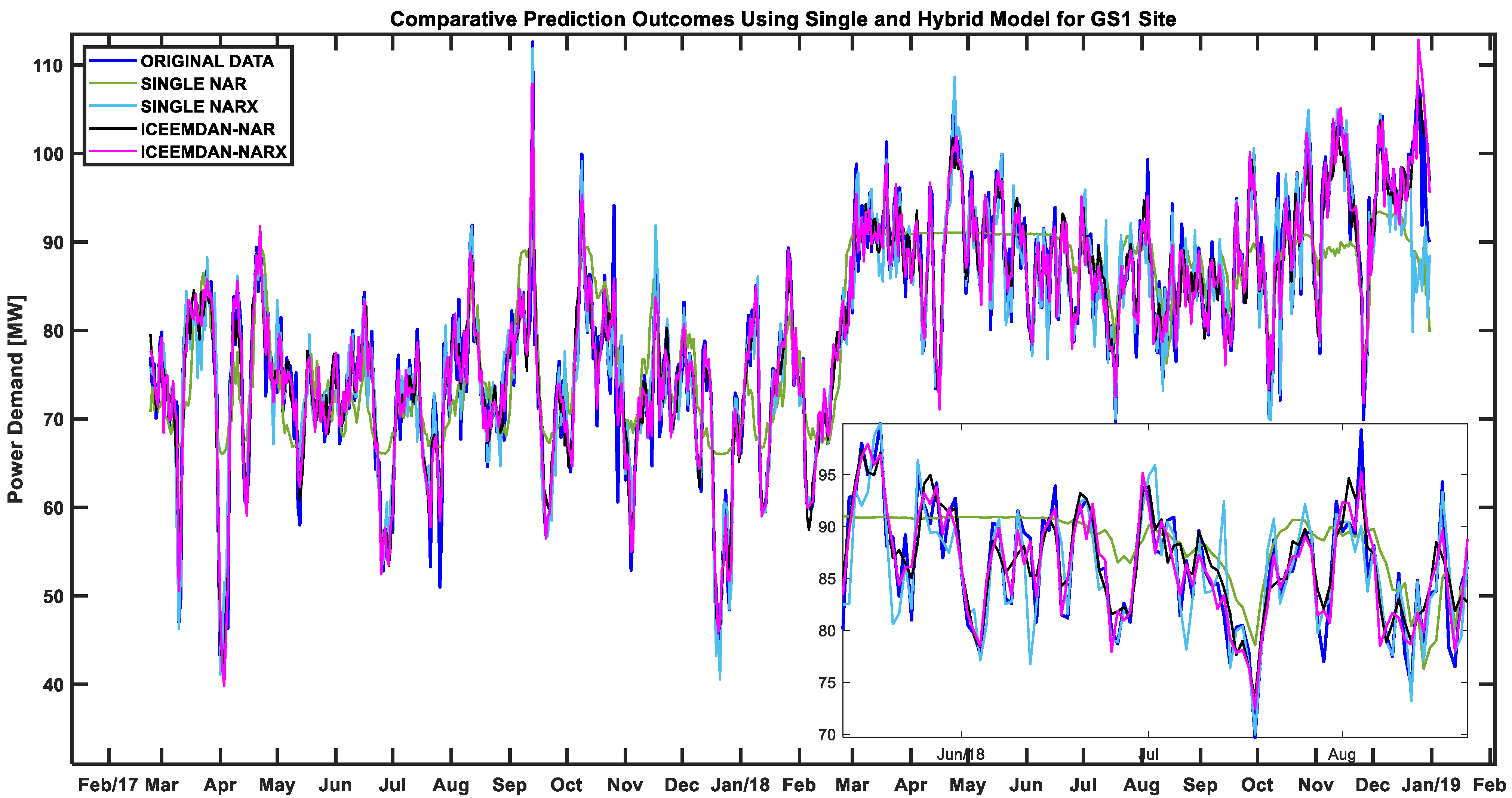
4.4. Hybrid Models
5. Discussion
5.1. Sensitivity to the Number of Climate Variables
5.2. Sensitivity to the Key Parameters in RNNs
6. Conclusions
Author Contributions
Funding
Data Availability Statement
Conflicts of Interest
Abbreviations
| AC | All correlated |
| ADB | Asian Development Bank |
| AFD | Adaptive Fourier decomposition |
| ANN | Artificial neural network |
| ARIMA | Autoregressive integrated moving average |
| BPNN | Back-propagation-based neural network |
| CEEMDAN | Complete ensemble empirical mode decomposition with adaptive noise |
| CNN | Convolution neural network |
| CO2 | Carbon dioxide |
| EAC | Electricity Authority of Cambodia |
| ECMWF | European Center for Medium-Range Weather Forecast |
| EDC | Electricité du Cambodge |
| EEMD | Ensemble empirical mode decomposition |
| EMD | Empirical mode decomposition |
| ExSS | Extended snapshot |
| FFNN | Feed-forward neural network |
| GDP | Gross domestic production |
| GS | Grid substation |
| HC | Highly correlated |
| HFO | Heavy fuel oil |
| HFT | Hidden transfer function |
| HHO | Harris hawks optimization |
| ICEEMDAN | Improved complete ensemble empirical mode decomposition with adaptive noise |
| IMF | Intrinsic mode function |
| LEAP | Long-range alternatives energy planning |
| LPG | Liquefied petroleum gas |
| LRF | Linear recurrent formula |
| LSSVM | Least-square-support vector machine |
| LSTM | Long–short-term memory network |
| MAE | Mean absolute error |
| MAPE | Mean absolute percentage error |
| MARS | Multivariate adaptive regression spline |
| ML | Machine learning |
| MLR | Multiple linear regression |
| NAR | Nonlinear autoregressive neural network |
| NARX | Nonlinear autoregressive neural network with exogenous inputs |
| NMSE | Normalized mean square error |
| OFT | Output transfer function |
| PDP | Power development plan |
| PSO | Particle swarm optimization |
| RMSE | Root-mean square error |
| RNN | Recurrent neural network |
| SCADA | Supervisory control and data acquisition |
| SDGs | Sustainable development goals |
| SSA | Singular spectrum analysis |
| SVR | Support vector regression |
| SWPT | Stationary wavelet packet transform decomposition |
| TCN | Temporal convolutional network |
| VMD | Variational mode decomposition |
| WAsP | Wind Atlas Analysis and Application Program |
| WPP | West Phnom Penh grid substation |
Appendix A. ERA5 Climate Variables


| Data Description | No. | Main Climate Variables | Acronym | Daily Dataset |
|---|---|---|---|---|
| Mean (1 January 2013) | ||||
| ERA5 climate reanalysis | 1 | Boundary layer dissipation | BLD | 4303.75 |
| 2 | Boundary layer height | BLH | 563.93 | |
| 3 | Convective available potential energy | CAPE | 0.04 | |
| 4 | CHNK | 0.02 | ||
| 5 | Convective precipitation | CP | 0.00 | |
| 6 | 2-metre dewpoint temperature | D | 292.15 | |
| 7 | Evaporation | E | 0.00 | |
| 8 | Eastward turbulent surface stress | EWSS | −109.38 | |
| 9 | Forecast albedo | FAL | 0.16 | |
| 10 | 10-metre wind gusts since previous postprocessing | FG10 | 6.12 | |
| 11 | Forecast logarithm of surface roughness for heat | FLSR | −3.84 | |
| 12 | Forecast surface roughness | FSR | 0.47 | |
| 13 | High cloud cover | HCC | 0.87 | |
| 14 | Instantaneous moisture flux | IE | 0.00 | |
| 15 | Instantaneous eastward turbulent surface stress | IEWS | −0.04 | |
| 16 | Instantaneous northward turbulent surface stress | INSS | −0.15 | |
| 17 | Instantaneous surface sensible heat flux | ISHF | −52.10 | |
| 18 | Low cloud cover | LCC | 0.17 | |
| 19 | Large-scale precipitation fraction | LSPF | 0.00 | |
| 20 | MCC | 0.06 | ||
| 21 | Mean sea level pressure | MSL | 101,139.75 | |
| 22 | Northward turbulent surface stress | NSSS | −528.31 | |
| 23 | Vertical integral of potential, internal, and latent energy | P62.162 | 2,780,152,438.89 | |
| 24 | Vertical integral of total energy | P63.162 | 2,780,456,503.09 | |
| 25 | Vertical integral of eastward kinetic energy flux | P67.162 | −1,832,177.66 | |
| 26 | Vertical integral of eastward geopotential flux | P73.162 | −2,982,667,364.29 | |
| 27 | Vertical integral of northward geopotential flux | P74.162 | 2,069,308,190.16 | |
| 28 | Vertical integral of eastward total energy flux | P75.162 | −14,986,239,992.45 | |
| 29 | Vertical integral of eastward ozone flux | P77.162 | 0.02 | |
| 30 | RO | 0.00 | ||
| 31 | Skin temperature | SKT | 300.50 | |
| 32 | Surface latent heat flux | SLHF | −286,915.24 | |
| 33 | SP | 100,833.20 | ||
| 34 | Skin reservoir content (m of water equivalent) | SRC | 0.00 | |
| 35 | Surface sensible heat flux | SSHF | −186,000.54 | |
| 36 | Surface net solar radiation | SSR | 692,607.54 | |
| 37 | Surface net solar radiation, clear sky | SSRC | 721,085.09 | |
| 38 | Surface net solar radiation, downwards | SSRD | 818,633.89 | |
| 39 | Soil temperature level 1 | STL1 | 301.93 | |
| 40 | Soil temperature level 2 | STL2 | 301.76 | |
| 41 | Soil temperature level 3 | STL3 | 302.18 | |
| 42 | Soil temperature level 4 | STL4 | 301.95 | |
| 43 | Surface net thermal radiation | STR | −222,398.82 | |
| 44 | Surface net thermal radiation, clear sky | STRC | −254,379.87 | |
| 45 | Surface thermal radiation, downwards | STRD | 1,435,890.80 | |
| 46 | Volumetric soil water layer 1 | SWVL1 | 0.21 | |
| 47 | Volumetric soil water layer 2 | SWVL2 | 0.22 | |
| 48 | Volumetric soil water layer 3 | SWVL3 | 0.29 | |
| 49 | Volumetric soil water layer 4 | SWVL4 | 0.29 | |
| 50 | T2 M | 300.33 | ||
| 51 | Total cloud cover | TCC | 0.88 | |
| 52 | Total column cloud liquid water | TCLW | 0.02 | |
| 53 | TCO3 | 0.00 | ||
| 54 | Total column cloud ice water | TCIW | 0.00 | |
| 55 | Total column water | TCW | 37.75 | |
| 56 | TCWV | 37.71 | ||
| 57 | TOA incident solar radiation | TISR | 1,260,279.10 | |
| 58 | Total precipitation | TP | 0.00 | |
| 59 | Temperature of snow layer | TSN | 273.05 | |
| 60 | Top net solar radiation | TSR | 1,009,476.83 | |
| 61 | Top net solar radiation, clear sky | TSRC | 1,043,013.34 | |
| 62 | Top net thermal radiation | TTR | −863,546.10 | |
| 63 | Top net thermal radiation, clear sky | TTRC | −1,037,561.45 | |
| 64 | 10-metre U wind component | U10 | −0.48 | |
| 65 | Downward U.V. radiation at the surface | UVB | 95,201.23 | |
| 66 | 10-metre V wind component | V10 | −2.65 |
References
- Thatcher, M.J. Modelling Changes to Electricity Demand Load Duration Curves as a Consequence of Predicted Climate Change for Australia. Energy 2007, 32, 1647–1659. [Google Scholar] [CrossRef]
- Wang, C.; Grozev, G.; Seo, S. Decomposition and Statistical Analysis for Regional Electricity Demand Forecasting. Energy 2012, 41, 313–325. [Google Scholar] [CrossRef]
- Abbas, F.; Feng, D.; Habib, S.; Rahman, U.; Rasool, A.; Yan, Z. Short Term Residential Load Forecasting: An Improved Optimal Nonlinear Auto Regressive (NARX) Method with Exponential Weight Decay Function. Electronics 2018, 7, 432. [Google Scholar] [CrossRef] [Green Version]
- Buitrago, J.; Asfour, S. Short-Term Forecasting of Electric Loads Using Nonlinear Autoregressive Artificial Neural Networks with Exogenous Vector Inputs. Energies 2017, 10, 40. [Google Scholar] [CrossRef] [Green Version]
- Netsanet, S.; Zhang, J.; Zheng, D. Short Term Load Forecasting Using Wavelet Augmented Non-Linear Autoregressive Neural Networks: A Single Customer Level Perspective. In Proceedings of the IEEE 3rd International Conference on Big Data Analysis (ICBDA), Shanghai, China, 9–12 March 2018; pp. 407–411. [Google Scholar] [CrossRef]
- Wunsch, A.; Liesch, T.; Broda, S. Forecasting Groundwater Levels Using Nonlinear Autoregressive Networks with Exogenous Input (NARX). J. Hydrol. 2018, 567, 743–758. [Google Scholar] [CrossRef]
- Zhou, Y.; Guo, S.; Xu, C.-Y.; Chang, F.-J.; Yin, J. Improving the Reliability of Probabilistic Multi-Step-Ahead Flood Forecasting by Fusing Unscented Kalman Filter with Recurrent Neural Network. Water 2020, 12, 578. [Google Scholar] [CrossRef] [Green Version]
- Cadenas, E.; Rivera, W.; Campos-Amezcua, R.; Cadenas, R. Wind Speed Forecasting Using the NARX Model, Case: La Mata, Oaxaca, México. Neural Comput. Applic. 2016, 27, 2417–2428. [Google Scholar] [CrossRef]
- Altan, A.; Karasu, S.; Zio, E. A New Hybrid Model for Wind Speed Forecasting Combining Long Short-Term Memory Neural Network, Decomposition Methods and Grey Wolf Optimizer. Appl. Soft Comput. 2021, 100, 106996. [Google Scholar] [CrossRef]
- Blanchard, T.; Samanta, B. Wind Speed Forecasting Using Neural Networks. Wind Eng. 2020, 44, 33–48. [Google Scholar] [CrossRef]
- Alzahrani, A.; Kimball, J.W.; Dagli, C. Predicting Solar Irradiance Using Time Series Neural Networks. Procedia Comput. Sci. 2014, 36, 623–628. [Google Scholar] [CrossRef] [Green Version]
- Boussaada, Z.; Curea, O.; Remaci, A.; Camblong, H.; Mrabet Bellaaj, N. A Nonlinear Autoregressive Exogenous (NARX) Neural Network Model for the Prediction of the Daily Direct Solar Radiation. Energies 2018, 11, 620. [Google Scholar] [CrossRef] [Green Version]
- Kazemzadeh, M.-R.; Amjadian, A.; Amraee, T. A Hybrid Data Mining Driven Algorithm for Long Term Electric Peak Load and Energy Demand Forecasting. Energy 2020, 204, 117948. [Google Scholar] [CrossRef]
- Ahmed, T.; Muttaqi, K.M.; Agalgaonkar, A.P. Climate Change Impacts on Electricity Demand in the State of New South Wales, Australia. Appl. Energy 2012, 98, 376–383. [Google Scholar] [CrossRef]
- Tayab, U.B.; Zia, A.; Yang, F.; Lu, J.; Kashif, M. Short-Term Load Forecasting for Microgrid Energy Management System Using Hybrid HHO-FNN Model with Best-Basis Stationary Wavelet Packet Transform. Energy 2020, 203, 117857. [Google Scholar] [CrossRef]
- AL-Musaylh, M.S.; Deo, R.C.; Adamowski, J.F.; Li, Y. Short-Term Electricity Demand Forecasting Using Machine Learning Methods Enriched with Ground-Based Climate and ECMWF Reanalysis Atmospheric Predictors in Southeast Queensland, Australia. Renew. Sustain. Energy Rev. 2019, 113, 109293. [Google Scholar] [CrossRef]
- Runge, J.; Zmeureanu, R.; Le Cam, M. Hybrid Short-Term Forecasting of the Electric Demand of Supply Fans Using Machine Learning. J. Build. Eng. 2020, 29, 101144. [Google Scholar] [CrossRef]
- Sulandari, W.; Subanar, S.S.; Lee, M.H.; Rodrigues, P.C. Indonesian Electricity Load Forecasting Using Singular Spectrum Analysis, Fuzzy Systems and Neural Networks. Energy 2020, 190, 116408. [Google Scholar] [CrossRef]
- Lee, H.-Y.; Jang, K.M.; Kim, Y. Energy Consumption Prediction in Vietnam with an Artificial Neural Network-Based Urban Growth Model. Energies 2020, 13, 4282. [Google Scholar] [CrossRef]
- Shen, Y.; Ma, Y.; Deng, S.; Huang, C.-J.; Kuo, P.-H. An Ensemble Model Based on Deep Learning and Data Preprocessing for Short-Term Electrical Load Forecasting. Sustainability 2021, 13, 1694. [Google Scholar] [CrossRef]
- Li, R.; Jiang, P.; Yang, H.; Li, C. A Novel Hybrid Forecasting Scheme for Electricity Demand Time Series. Sustain. Cities Soc. 2020, 55, 102036. [Google Scholar] [CrossRef]
- Bedi, J.; Toshniwal, D. Deep Learning Framework to Forecast Electricity Demand. Appl. Energy 2019, 238, 1312–1326. [Google Scholar] [CrossRef]
- Kandananond, K. Forecasting Electricity Demand in Thailand with an Artificial Neural Network Approach. Energies 2011, 4, 1246–1257. [Google Scholar] [CrossRef] [Green Version]
- Jaisumroum, N.; Teeravaraprug, J. Forecasting Uncertainty of Thailand’s Electricity Consumption Compare with Using Artificial Neural Network and Multiple Linear Regression Methods. In Proceedings of the 12th IEEE Conference on Industrial Electronics and Applications (ICIEA), Siem Reap, Cambodia, 18–20 June 2017; pp. 308–313. [Google Scholar] [CrossRef]
- Bantugon, M.J.T.; Gallano, R.J.C. Short- and Long-Term Electricity Load Forecasting Using Classical and Neural Network Based Approach: A Case Study for the Philippines. In Proceedings of the IEEE Region 10 Conference (TENCON), Singapore, 22–26 November 2016; pp. 3822–3825. [Google Scholar] [CrossRef]
- World Bank Group. Cambodia Economic Update. 2019. Available online: https://documents1.worldbank.org/curated/en/707971575947227090/pdf/Cambodia-Economic-Update-Upgrading-Cambodia-in-Global-Value-Chains.pdf (accessed on 23 May 2021).
- MME. Power Development Master Plan (PDP) (Power Development Master Plan in Kingdom of Cambodia); MME: Phnom Penh, Cambodia, 2015. [Google Scholar]
- ADB. Cambodia: Energy Sector Assessment, Strategy, and Road Map. 2018. Available online: http://0-search-ebscohost-com.brum.beds.ac.uk/login.aspx?direct=true&scope=site&db=nlebk&db=nlabk&AN=2029528 (accessed on 23 April 2021).
- EAC. Salient Feature of Power Development in the Kindom of Cambodia Until December 2019; EAC: Phnom Penh, Cambodia, 2019. [Google Scholar]
- Lyheang, C.; Limmeechokchai, B. The Role of Renewable Energy in CO2 Mitigation from Power Sector in Cambodia. Int. Energy J. 2018, 18. Available online: http://www.rericjournal.ait.ac.th/index.php/reric/article/view/1970 (accessed on 11 June 2021).
- San, V.; Sriv, T.; Spoann, V.; Var, S.; Seak, S. Economic and Environmental Costs of Rural Household Energy Consumption Structures in Sameakki Meanchey District, Kampong Chhnang Province, Cambodia. Energy 2012, 48, 484–491. [Google Scholar] [CrossRef]
- Hak, M.; Matsuoka, Y.; Gomi, K. A Qualitative and Quantitative Design of Low-Carbon Development in Cambodia: Energy Policy. Energy Policy 2017, 100, 237–251. [Google Scholar] [CrossRef]
- Promsen, W.; Janjai, S.; Tantalechon, T. An Analysis of Wind Energy Potential of Kampot Province, Southern Cambodia. Energy Procedia 2014, 52, 633–641. [Google Scholar] [CrossRef] [Green Version]
- EDC. Annual Report 2013; EDC: Phnom Penh, Cambodia, 2013; Available online: http://edc.com.kh/images/Annual%20Report%202013%20Publish.pdf (accessed on 23 February 2021).
- EDC. Annual Report 2017; EDC: Phnom Penh, Cambodia, 2017; Available online: http://edc.com.kh/images/Annual%20Report%202017%20(English)__pdf (accessed on 4 February 2021).
- EAC. Annual Report on Power Sector for Year 2019; EAC: Phnom Penh, Cambodia, 2019. Available online: https://eac.gov.kh/uploads/annual_report/english/Annual-Report-2019-en.pdf (accessed on 31 July 2020).
- Su, T.; Shi, Y.; Yu, J.; Yue, C.; Zhou, F. Nonlinear Compensation Algorithm for Multidimensional Temporal Data: A Missing Value Imputation for the Power Grid Applications. Knowl. -Based Syst. 2021, 215, 106743. [Google Scholar] [CrossRef]
- Li, M.; Yang, B.; Zhai, W.; Ma, X.; Xia, Y.; Lin, Y. Non-Mechanism Model for Superheater Pollution Diagnosis of Waste Incinerator Based on BP Neural Network. IOP Conf. Ser. Mater. Sci. Eng. 2019, 612, 052015. [Google Scholar] [CrossRef]
- Abidoye, L.K.; Mahdi, F.M.; Idris, M.O.; Alabi, O.O.; Wahab, A.A. ANN-Derived Equation and ITS Application in the Prediction of Dielectric Properties of Pure and Impure CO2. J. Clean. Prod. 2018, 175, 123–132. [Google Scholar] [CrossRef]
- Lee, H.S. Improvement of Decomposing Results of Empirical Mode Decomposition and Its Variations for Sea-Level Records Analysis. J. Coast. Res. 2018, 85, 526–530. [Google Scholar] [CrossRef]
- Huang, N.E.; Shen, Z.; Long, S.R.; Wu, M.C.; Shih, H.H.; Zheng, Q.; Yen, N.-C.; Tung, C.C.; Liu, H.H. The Empirical Mode Decomposition and the Hilbert Spectrum for Nonlinear and Non-Stationary Time Series Analysis. Proc. R. Soc. Lond. A 1998, 454, 903–995. [Google Scholar] [CrossRef]
- Wu, Z.; Huang, N.E. Ensemble Empirical Mode Decomposition: A Noise-Assisted Data Analysis Method. Adv. Adapt. Data Anal. 2009, 1, 1–41. [Google Scholar] [CrossRef]
- Colominas, M.A.; Schlotthauer, G.; Torres, M.E.; Flandrin, P. NOISE-ASSISTED EMD METHODS IN ACTION. Adv. Adapt. Data Anal. 2012, 4, 1250025. [Google Scholar] [CrossRef] [Green Version]
- Torres, M.E.; Colominas, M.A.; Schlotthauer, G.; Flandrin, P. A Complete Ensemble Empirical Mode Decomposition with Adaptive Noise. In Proceedings of the 2011 IEEE International Conference on Acoustics, Speech and Signal Processing (ICASSP), Prague, Czech Republic, 22–27 May 2011; IEEE: Prague, Czech Republic, 2011; pp. 4144–4147. [Google Scholar] [CrossRef]
- Colominas, M.A. Improved Complete Ensemble EMD: A Suitable Tool for Biomedical Signal Processing. Biomed. Signal Process. Control 2014, 14, 19–29. [Google Scholar] [CrossRef]
- Yang, S.; Yang, D.; Chen, J.; Zhao, B. Real-Time Reservoir Operation Using Recurrent Neural Networks and Inflow Forecast from a Distributed Hydrological Model. J. Hydrol. 2019, 579, 124229. [Google Scholar] [CrossRef]
- Zhang, G.; Zhou, H.; Wang, C.; Xue, H.; Wang, J.; Wan, H. Forecasting Time Series Albedo Using NARnet Based on EEMD Decomposition. IEEE Trans. Geosci. Remote Sens. 2020, 58, 3544–3557. [Google Scholar] [CrossRef]
- Khalid, A.; Sundararajan, A.; Sarwat, A.I. A Multi-Step Predictive Model to Estimate Li-Ion State of Charge for Higher C-Rates. In Proceedings of the IEEE International Conference on Environment and Electrical Engineering and 2019 IEEE Industrial and Commercial Power Systems Europe (EEEIC/I&CPS Europe), Genova, Italy, 11–14 June 2019; pp. 1–6. [Google Scholar] [CrossRef]
- Di Piazza, A.; Di Piazza, M.C.; La Tona, G.; Luna, M. An artificial neural network-based forecasting model of energy-related time series for electrical grid management. Math. Comput. Simul. 2021, 184, 294–305. [Google Scholar] [CrossRef]
- Ryu, J.-A.; Chang, S. Data Driven Heating Energy Load Forecast Modeling Enhanced by Nonlinear Autoregressive Exogenous Neural Networks. IJSCER 2019, 8, 246–252. [Google Scholar] [CrossRef]
- Kumar, D.A.; Murugan, S. Performance Analysis of NARX Neural Network Backpropagation Algorithm by Various Training Functions for Time Series Data. IJDS 2018, 3, 308. [Google Scholar] [CrossRef]
- Sarkar, R.; Julai, S.; Hossain, S.; Chong, W.T.; Rahman, M. A Comparative Study of Activation Functions of NAR and NARX Neural Network for Long-Term Wind Speed Forecasting in Malaysia. Math. Probl. Eng. 2019, 2019, 1–14. [Google Scholar] [CrossRef]
- Vogl, T.P.; Mangis, J.K.; Rigler, A.K.; Zink, W.T.; Alkon, D.L. Accelerating the Convergence of the Back-Propagation Method. Biol. Cybern. 1988, 59, 257–263. [Google Scholar] [CrossRef]
- Li, Q.; Liang, S.; Yang, J.; Li, B. Long Range Dependence Prognostics for Bearing Vibration Intensity Chaotic Time Series. Entropy 2016, 18, 23. [Google Scholar] [CrossRef] [Green Version]
- Hussainzada, W.; Lee, H.S.; Vinayak, B.; Khpalwak, G.F. Sensitivity of Snowmelt Runoff Modelling to the Level of Cloud Coverage for Snow Cover Extent from Daily MODIS Product Collection 6. J. Hydrol. Reg. Stud. 2021, 36, 100835. [Google Scholar] [CrossRef]
- Mohammadi, K.; Shamshirband, S.; Tong, C.W.; Arif, M.; Petković, D.; Ch, S. A New Hybrid Support Vector Machine–Wavelet Transform Approach for Estimation of Horizontal Global Solar Radiation. Energy Convers. Manag. 2015, 92, 162–171. [Google Scholar] [CrossRef]
- Prasad, R.; Deo, R.C.; Li, Y.; Maraseni, T. Input Selection and Performance Optimization of ANN-Based Streamflow Forecasts in the Drought-Prone Murray Darling Basin Region Using IIS and MODWT Algorithm. Atmos. Res. 2017, 197, 42–63. [Google Scholar] [CrossRef]
- Guiamel, I.A.; Lee, H.S. Watershed Modelling of the Mindanao River Basin in the Philippines Using the SWAT for Water Resource Management. Civ. Eng. J. 2020, 6, 626–648. [Google Scholar] [CrossRef]


| Substation Name | Power Demand | ERA5 Reanalysis | ||||||
|---|---|---|---|---|---|---|---|---|
| Latitude | Longitude | Peak | Mean | Latitude | Longitude | Temporal Resolution | Horizontal Resolution | |
| GS1 | 11.58989 | 104.91545 | 158.20 | 81.93 | 11.60 | 104.90 | Hourly | 0.1° × 0.1° Native resolution is 9 km |
| GS2 | 11.52899 | 104.92944 | 167.10 | 91.13 | 11.60 | 104.90 | ||
| GS3 | 11.55495 | 104.88438 | 145.20 | 76.25 | 11.60 | 104.90 | ||
| WPP | 11.39941 | 104.77168 | 199.00 | 51.94 | 11.40 | 104.80 | ||
| Rank | Description | Performance Ratting |
|---|---|---|
| 1 | R2 ≥ 0.80 | Excellent |
| 2 | 0.70 < R2 < 0.60 | Good |
| 3 | 0.60 < R2 < 0.50 | Satisfactory |
| 4 | R2 ≤ 0.50 | Not satisfactory |
| Model | NMSE | MAE (MW) | RMSE (MW) | MAPE (%) | |
|---|---|---|---|---|---|
| Stand-alone NAR | 14.65 | 0.678 | 5.192 | 6.745 | 0.435 |
| Stand-alone NARX | 1.343 | 0.902 | 2.288 | 3.713 | 0.432 |
| Model | NAR | NARX | ||||||||
|---|---|---|---|---|---|---|---|---|---|---|
| NMSE | MAE (MW) | RMSE (MW) | MAPE (%) | NMSE | MAE (MW) | RMSE (MW) | MAPE (%) | |||
| Stand-alone model | 14.65 | 0.678 | 5.192 | 6.745 | 0.435 | 1.343 | 0.902 | 2.288 | 3.713 | 0.432 |
| IMF1 | 7.238 | 0.122 | 2.225 | 2.868 | 85.850 | 3.904 | 0.359 | 1.869 | 2.464 | 63.230 |
| IMF2 | 0.173 | 0.838 | 0.787 | 1.030 | 15.330 | 0.007 | 0.969 | 0.184 | 0.466 | 0.158 |
| IMF3 | 0.026 | 0.952 | 0.421 | 0.733 | 2.898 | 0.0003 | 0.995 | 0.044 | 0.251 | 0.074 |
| IMF4 | 0.010 | 0.974 | 0.429 | 0.604 | 1.947 | 0.004 | 0.981 | 0.056 | 0.490 | 0.381 |
| IMF5 | 0.003 | 0.978 | 0.281 | 0.387 | 8.677 | 3.95 × 10−³ | 0.999 | 0.010 | 0.039 | 0.299 |
| IMF6 | 0.016 | 0.952 | 0.421 | 0.583 | 15.785 | 6.23 × 10⁻⁹ | 0.999 | 0.003 | 0.016 | 0.105 |
| IMF7 | 0.007 | 0.962 | 0.329 | 0.457 | 5.953 | 5.07 × 10⁻⁷ | 0.999 | 0.005 | 0.040 | 0.006 |
| IMF8 | 0.004 | 0.961 | 0.360 | 0.411 | 11.361 | 3.06 × 10⁻¹¹ | 0.999 | 0.001 | 0.004 | 0.004 |
| IMF9 | 0.052 | 0.952 | 1.024 | 1.144 | 20.868 | 2.68 × 10⁻¹¹ | 0.999 | 0.002 | 0.006 | 0.014 |
| Residue | 0.096 | 0.898 | 0.980 | 1.089 | 0.402 | 1.65 × 10⁻¹³ | 0.999 | 0.001 | 0.001 | 5.62 × 10⁻⁵ |
| Hybrid model | 0.074 | 0.926 | 2.519 | 3.240 | 0.214 | 0.048 | 0.952 | 1.923 | 2.605 | 0.032 |
| Model | ||||||||||
|---|---|---|---|---|---|---|---|---|---|---|
| NMSE | MAE (MW) | RMSE (MW) | MAPE (%) | NMSE | MAE (MW) | RMSE (MW) | MAPE (%) | |||
| Stand-alone model | 3.989 | 0.830 | 3.814 | 4.897 | 0.354 | 1.343 | 0.902 | 2.288 | 3.713 | 0.432 |
| IMF1 | 6.396 | 0.1737 | 2.092 | 2.783 | 81.16 | 3.904 | 0.359 | 1.869 | 2.464 | 63.230 |
| IMF2 | 0.020 | 0.944 | 0.390 | 0.5938 | 6.383 | 0.007 | 0.969 | 0.184 | 0.466 | 0.158 |
| IMF3 | 0.003 | 0.983 | 0.193 | 0.431 | 0.674 | 0.0003 | 0.995 | 0.044 | 0.251 | 0.074 |
| IMF4 | 9.58 × 10⁻⁷ | 0.999 | 0.039 | 0.061 | 0.011 | 0.004 | 0.981 | 0.056 | 0.490 | 0.381 |
| IMF5 | 1.05 × 10⁻⁷ | 0.999 | 0.011 | 0.029 | 0.128 | 3.95 × 10⁻⁷ | 0.999 | 0.010 | 0.039 | 0.299 |
| IMF6 | 1.27 × 10⁻¹⁰ | 0.999 | 0.002 | 0.005 | 0.026 | 6.23 × 10⁻⁹ | 0.999 | 0.003 | 0.016 | 0.105 |
| IMF7 | 9.99 × 10⁻⁵ | 0.996 | 0.115 | 0.1624 | 0.470 | 5.07 × 10⁻⁷ | 0.999 | 0.005 | 0.040 | 0.006 |
| IMF8 | 5.05 × 10⁻¹¹ | 0.999 | 0.003 | 0.004 | 0.004 | 3.06 × 10⁻¹¹ | 0.999 | 0.001 | 0.004 | 0.004 |
| IMF9 | 1.76 × 10⁻⁷ | 0.999 | 0.038 | 0.045 | 0.042 | 2.68 × 10⁻¹¹ | 0.999 | 0.002 | 0.006 | 0.014 |
| Residue | 9.13 × 10⁻¹³ | 0.999 | 0.001 | 0.002 | 2.4 × 10⁻⁴ | 1.65 × 10⁻¹³ | 0.999 | 0.001 | 0.001 | 5.62 × 10⁻⁵ |
| Hybrid model | 0.062 | 0.937 | 2.225 | 2.967 | 0.302 | 0.048 | 0.952 | 1.923 | 2.605 | 0.032 |
Publisher’s Note: MDPI stays neutral with regard to jurisdictional claims in published maps and institutional affiliations. |
© 2022 by the authors. Licensee MDPI, Basel, Switzerland. This article is an open access article distributed under the terms and conditions of the Creative Commons Attribution (CC BY) license (https://creativecommons.org/licenses/by/4.0/).
Share and Cite
Chreng, K.; Lee, H.S.; Tuy, S. A Hybrid Model for Electricity Demand Forecast Using Improved Ensemble Empirical Mode Decomposition and Recurrent Neural Networks with ERA5 Climate Variables. Energies 2022, 15, 7434. https://0-doi-org.brum.beds.ac.uk/10.3390/en15197434
Chreng K, Lee HS, Tuy S. A Hybrid Model for Electricity Demand Forecast Using Improved Ensemble Empirical Mode Decomposition and Recurrent Neural Networks with ERA5 Climate Variables. Energies. 2022; 15(19):7434. https://0-doi-org.brum.beds.ac.uk/10.3390/en15197434
Chicago/Turabian StyleChreng, Karodine, Han Soo Lee, and Soklin Tuy. 2022. "A Hybrid Model for Electricity Demand Forecast Using Improved Ensemble Empirical Mode Decomposition and Recurrent Neural Networks with ERA5 Climate Variables" Energies 15, no. 19: 7434. https://0-doi-org.brum.beds.ac.uk/10.3390/en15197434