Performance of Two Variable Machine Learning Models to Forecast Monthly Mean Diffuse Solar Radiation across India under Various Climate Zones

Abstract

For the various climatic zones of India, machine learning (ML) models are created in the current work to forecast monthly-average diffuse solar radiation (DSR). The long-term solar radiation data are taken from Indian Meteorological Department (IMD), Pune, provided for 21 cities that span all of India’s climatic zones. The diffusion coefficient and diffuse fraction are the two groups of ML models with dual input parameters (sunshine ratio and clearness index) that are built and compared (each category has seven models). To create ML models, two well-known ML techniques, random forest (RF) and k-nearest neighbours (KNN), are used. The proposed ML models are compared with well-known models that are found in the literature. The ML models are ranked according to their overall and within predictive power using the Global Performance Indicator (GPI). It is discovered that KNN models generally outperform RF models. The results reveal that in diffusion coefficient models perform well than diffuse fraction models. Moreover, functional form 2 is the best followed by form 6. The ML models created here can be effectively used to accurately forecast DSR in various climates.

1. Introduction

Proper exertion of energy resources is a major issue these days. It is essential to be concerned about which energy source must be applied and why. Cleanliness, cost, stability, efficiency and environmental effects are a few things that need to be considered. Moreover, many industries worldwide still depend on fossil fuels for the generation of electricity. Of course, these fuels are very effective as far as the power production quality is concerned, but it is not easy to depend on them for a long period. One day, fossil fuels will be depleted. Industries must rely on renewable resources to solve this problem. Additionally, fossil fuels pose a serious threat to the environment’s balance and have numerous ecological issues [1].

Solar energy is widely accessible and abundant all year in India. There are 2776 h of total daily sunshine in India, and the average annual global solar radiation (GSR) is 5.25 kWh/m²-day [2,3]. In some areas of North India, the greatest energy availability during the summer is 7.5 kWh/m²/day [4].

For performance estimation, planning and execution, solar thermal systems require precise data on the solar radiation potential [5,6,7,8,9,10]. A specific site’s solar radiation potential can be assessed using the radiation data, modelling and forecasting methods that are now available [11]. The only cities for which these data are available in a country such as India are the metro areas [12]. Although smaller cities have a significant solar energy potential as well, this information is typically unavailable due to the significant cost associated with establishing metrological facilities. Solar radiation models can be quite helpful in these circumstances. It is possible to model horizontal diffuse solar radiation using a variety of methods.

Diffuse solar radiation modelling was the subject of early ground-breaking efforts by Reindl et al. [13,14], Angström [15], Iqbal [16] and Liu and Jordan [17]. The researchers have provided various empirical models with clearness index as an input (linear, polynomial, exponential, log and power law). Models based on temperature, relative sunshine, relative humidity and climatic variables were also suggested by researchers [18,19]. Al-Mohamad [20], Noorian et al. [21], Diez-Mediavilla et al. [22], Tarhan and Sari [23], Aras et al. [24] and many more researchers also applied these techniques. According to studies by Boland et al. [25], El-Sebaii et al. [26], Haydar et al. [24], Iqbal [27] and Boland et al. [28], diffuse fraction and sunshine duration were related. Few researchers, according to Gopinathan [29], El-Sebaii and Trabea [30] and Jiang [31], select both the clearness index and the duration of sunshine.

Fourteen models were created and compared by Wattan and Janjai [32] at two different tropical locations. Eight models were proposed by Ulgen and Hepbasli [33] for the DSR forecast for Turkey. For Trabzon, Turkey, Kaygusuz [34] has found seven empirical relationships that can predict DSR. Bakirci [35] presented six models to forecast the monthly average DSR for Erzurum, Turkey, using a similar methodology. Eight models were created by Blaga [36] for the estimation of hourly DSR. In order to determine the solar energy potential in the Azores, Maggareiro et al. [37] evaluated the performance of various DSR models. New correlations were proposed by Li et al. [38] to anticipate China’s monthly mean daily DSR. For Kerman (Iran), Safaripour and Mehrabian [39] created models to predict horizontal DSR and GSR using linear regression analysis. In Rio de Janeiro, Filho et al. [40] classified solar radiation and created models to forecast GSR, DSR and BSR. Despotovic et al. [41] examined DSR models that were already in use from 267 sites around the globe that covered different climatic zones.

Many researchers, including Soares et al. [42], Ozan and Tuncay [43], Khatib et al. [44], Rehman and Mohanes [45], utilised the techniques of Artificial Neural Network (ANN) for calculating DSR. Machine Learning (ML) approaches have recently proved to predict solar radiation accurately by utilising different variables input that is accessible from weather stations [46]. Some input variables that can be used are daily global radiation, latitude, longitude, sunshine duration, temperature, wind velocity and wind direction [47]. Various ML algorithms can use different input variables to extract data from them. Support Vector Machines Regression [13,48,49], neural networks with different types [50,51], Gaussian processes [52], hybrid methodologies and a mix of these and alternative procedures [53,54,55,56,57,58] are a few of the ML techniques that researchers have reported. It has been noted in all instances that ML approaches produced excellent results in solar radiation prediction.

DSR modelling has been performed by several researchers in the Indian context. Modi and Sukhatme [59] showed that city-specific weather data, such as sunshine hours and precipitation, are the best predictors of day-to-day DSR. They asserted that as compared to daily DSR models, monthly average models provide better predictions. Muneer and Hawas [60] assessed the relationships between the monthly averaging values of GSR and DSR. Veeran and Kumar [61] observed a correlation between the daily mean DSR and monthly average clearness index. Parishad et al. [62] determine the constants necessary for the hourly GSR, BSR and DSR calculations in India. For various climatic zones in India, Jamil and Siddiqui [63] provided generalised models for DSR as a function of clearness index and associated sunshine duration. Jamil and Akhtar [64] conducted a comparison of hundred monthly average DSR models based on solar radiation measurements for the Indian city of Aligarh.

The literature review shows that most of the empirical correlations to estimate DSR are with a single input (clearness index or sunshine ratio). Though two-variable models have better estimation capability, only a few researchers have developed two-variable empirical models. Furthermore, the ML technique provides much better estimation in comparison to empirical models. Thus, in the present work, we want to combine the ML technique with two input predictors to obtain much better estimations of DSR. The different functional forms of the dual input (clearness index or sunshine ratio) are also compared. Development and comparison of ML models for the forecasting of monthly average DSR with two input predictors for various climate zones in India is the main goal of the current effort. In two categories, fourteen models with two input predictors are created (diffusion coefficient and diffuse fraction). Additionally, K-nearest neighbours (KNN) and Random Forest (RF), two ML approaches, are used in each category as suggested by Husain et al. [65]. Consequently, a total of 28 models are created. The data (obtained for IMD, Pune) are separated into training and validation sets, with training sets being used for model development and validating sets being used for model testing. Global Performance Index (GPI) is used to grade models for assessment accuracy within each group as well as within the group of 28 models.

2. Methodology and Data Description

2.1. Data for Solar Radiation

The current analysis covers all of India’s climatic zones. According to the Koppen classification [66], the six climatic regions of India are categorised as follows: montane, humid subtropical, tropical wet and dry, tropical wet, semi-arid and arid. We have chosen 21 cities, depicted on the map of India [66] in Figure 1 that covers all the climatic zones.

Table 1. Geographical coordinates of the designated cities.

S. No.	Location	Altitude (m)	Latitude	Longitude
1.	Srinagar	1587	34″08′	74″50′
2.	New Delhi	225	28″29′	77″08′
3.	Jaipur	431	26″49′	75″48′
4.	Jodhpur	231	26″18′	73″01′
5.	Patna	53	25″36′	85″10′
6.	Varanasi	81	25″18′	83″01′
7.	Ranchi	651	23″19′	85″19′
8.	Bhopal	500	23″17′	77″21′
9.	Gandhinagar	81	23″04′	72″38′
10.	Kolkata	14	22″39′	77″21′
11.	Bhavnagar	24	21″45′	72″11′
12.	Nagpur	310	21″06′	79″03′
13.	Mumbai	6	19″07′	72″51′
14.	Pune	560	18″32′	73″51′
15.	Vishakhapatnam	33	17″41′	83″81′
16.	Hyderabad	571	17″28′	78″28′
17.	Chennai	9	13″00′	80″11′
18.	Bangalore	911	12″58′	77″35′
19.	Port Blair	16	11″40′	92″43′
20.	Thiruvananthapuram	10	08″29′	76″57′
21.	Minicoy	2	08″18′	73″09′

displays the latitudes and longitudes of each place. The long-term solar radiation (1986–2000) data, which include monthly DSR, air temperature and sunshine hours, for these places, were obtained by IMD, Pune [67].

The following calculation is used to compute the average daily extra-terrestrial radiation (H₀) for each month:

$${\overline{H}}_0=\frac{24}{\pi }{H}_{sc}\left[1+0.033cos\left(\frac{360}{365}n\right)\right]\left[cos\varnothing cos\delta sin{\omega }_s+\frac{\pi }{180}sin\varnothing sin\delta \right]$$

(1)

where $H_{sc}$ is the solar constant, n is the day of the year that may be determined from Klien [68], $\varnothing$ is the latitude, ${\omega }_s$ is the angle at which the sun sets on a given day, $\delta$ is solar declination. The ensuing equations result in $\delta$ and ${\omega }_s$

$$\delta ={23.45}^{\mathrm{o}}sin\left[\frac{360(284+n}{365}\right]$$

(2)

$$cos{\omega }_s=-tan\varnothing tan\delta$$

(3)

2.2. Methodology

The modelling of the monthly average diffuse fraction (or diffusion coefficient) with monthly average clearness index and sunshine time as an input is necessary for DSR prediction [69].

The general equations for two categories of models are as follows:

$$\mathrm{Category}-1:\mathrm{Diffuse}\mathrm{fraction}{\overline{D}}_f=f\left(\overline{K_t},\overline{\theta }\right)$$

(4)

$$\mathrm{Category}-2:\mathrm{Diffusion}\mathrm{coefficient}{\overline{D}}_c=f\left(\overline{K_t},\overline{\theta }\right)$$

(5)

where ${\overline{D}}_f=\frac{\overline{H_d}}{\overline{H}}$ is diffuse fraction, ${\overline{D}}_c=\frac{\overline{H_d}}{\overline{H_0}}$ is diffusion coefficient, ${\overline{K}}_t=\frac{\overline{H}}{\overline{H_0}}$ is clearness index and $\overline{\theta }=\frac{\overline{S}}{\overline{S_0}}$ is sunshine ratio.$\overline{H},{\overline{H}}_0\mathrm{and}{\overline{H}}_d$ are, on a horizontal surface, monthly averages of GSR, ETSR and DSR, respectively. while $\overline{S}$ is actual sunshine hours and ${\overline{S}}_0$ is maximum possible sunshine hours can be obtained from:

$${\overline{S}}_o=\left(\raisebox{1ex}{$2$}\!\left/ \!\raisebox{-1ex}{$15$}\right.\right){\omega }_s$$

(6)

2.3. Statistical Indicators

A handful of the most widely used statistical measures were used to evaluate how well the developed ML models worked. They are the Uncertainty at 95% (U95), Mean Absolute Percentage Error (MAPE), Mean Bias Error (MBE), Root Mean Square Error (RMSE), Correlation Coefficient (R²) and Mean Bias Error (MBE). Details of the statistical indicators are provided in

Table 2. Mathematical equations of Statistical indicators employed in the current study.

S. No.	Statistical Indicator	Equation
1	Mean Bias Error (MBE)	$MBE=\frac{1}{n}{{\displaystyle \sum }}_{i=1}^n\left(E_i-M_i\right)$
2	Coefficient of Determination (R2)	$R^2=1-\frac{{{\displaystyle \sum }}_{i=1}^n{\left(M_i-E_i\right)}^2}{{{\displaystyle \sum }}_{i=1}^n\left(M_i-M_{avg}\right)}\times 100$
3	Root Mean Square Error (RMSE)	$RMSE=\sqrt{\frac{1}{n}{{\displaystyle \sum }}_{i=1}^n{\left(E_i-M_i\right)}^2}$
4	Mean Absolute Percentage error (MAPE)	$MAPE=\frac{100}{m}{{\displaystyle \sum }}_{i=1}^m\left|\frac{\left(E_i-M_i\right)}{M_i}\right|$
5	Uncertainty at 95% (U95)	$U_{95}=1.96{\left(S{D}^2+RMS{E}^2\right)}^{0.5}$

.

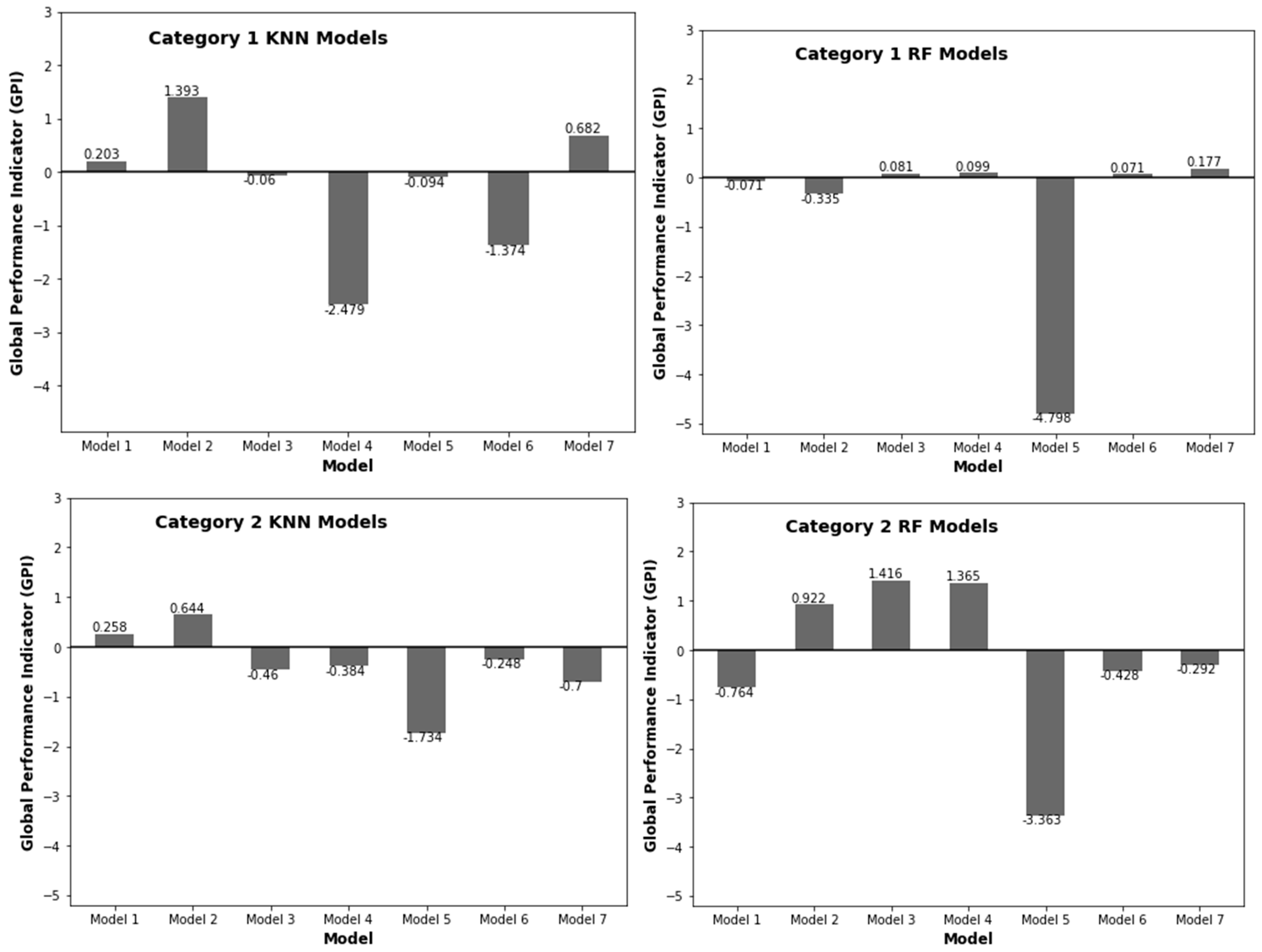
2.4. Global Performance Indicator (GPI)

Knowing which generated ML models outperform the others is pretty intriguing. To enhance our findings and eliminate any discrepancies that might have existed in the statistical analysis, we used GPI. Despotovic et al. [70] credited with initially introducing the innovative element known as GPI. It is an amazing method for combining the effects of many statistical pointers. All statistical pointers are scaled down between 0 and 1 during the process. The appropriate median value of all models is then subtracted from each scaled value of a statistical pointer. After that, the distinctions are combined with the proper weighting factors (−1 for R² and 1 for all other statistical pointers). The following is the equation for the kth model’s GPI:

$$GP{I}_k={{\displaystyle \sum }}_{i=i}^5{\alpha }_i\left({\tilde{y}}_i-{\tilde{y}}_{ki}\right)$$

(7)

where, ${\alpha }_i$ = weight factor. ${\tilde{y}}_i$ indicates the median for the scaled values of pointer i, the scaled value of pointer i for model k is shown by ${\tilde{y}}_{ki}$. The model with the highest GPI value is the one that is most accurate.

2.5. Machine Learning Models

In the current work, two ML regression techniques viz. K-nearest neighbours (KNN) [71] and Random Forest (RF) [72] are used.

K-Nearest Neighbours (KNN): One of the simpler ML algorithms is this one. Both classification and regression can be performed with it. When determining the mean value in comparison to the farthest neighbour, it operates under the premise that the closer neighbour contributes more. The weight of the neighbour will be 1/d if d is the distance between the node and the neighbour (Alfadda et al. [73]). The dataset’s distance to each test point $\widehat{x}$ and each training data point $x_i$ should be calculated as follows:

$$D_i\left(x,x_i\right)=\sqrt{{{\displaystyle \sum }}_j{\left(x_i^j-{\widehat{x}}^j\right)}^2}$$

(8)

For each test point $\widehat{x}$ the distance to all training points $x_i$ is computed, then the k nearest neighbour’s label values $y_i$ are averaged to predict the $\widehat{x}$ label value $\widehat{y}$.

Random Forest (RF): In an RF regression problem, we aggregate all of the high-variance trees so that the resulting variance is minimal, allowing each decision tree to be optimally trained on any sample data and, as a result, causing the output to depend on numerous trees rather than just one tree. In comparison, the average of all the outputs will be the ultimate result Breiman [74]. The entire description of RF is available in Feng, Cui, et al. [75].

For an ensemble of classifiers $h_1\left(x\right)$, $h_2\left(x\right) ,\dots ,h_k\left(x\right)$ and with the training dataset drawn at random from the distribution of the random vector $X$, $Y$, the margin function is expressed as:

$$mg\left(X,Y\right)=a{v}_{k}I\left(h_k\left(X\right)=Y\right)-ma{x}_{j\ne Y} a{v}_{k}I\left(h_k\left(X\right)=j\right)$$

(9)

3. Result and Discussion

Twenty-eight models in two categories were developed in the current study utilising two ML regression approaches. A few well-known models from the literature are selected for comparison with the newly constructed ML models proposed in the present work.

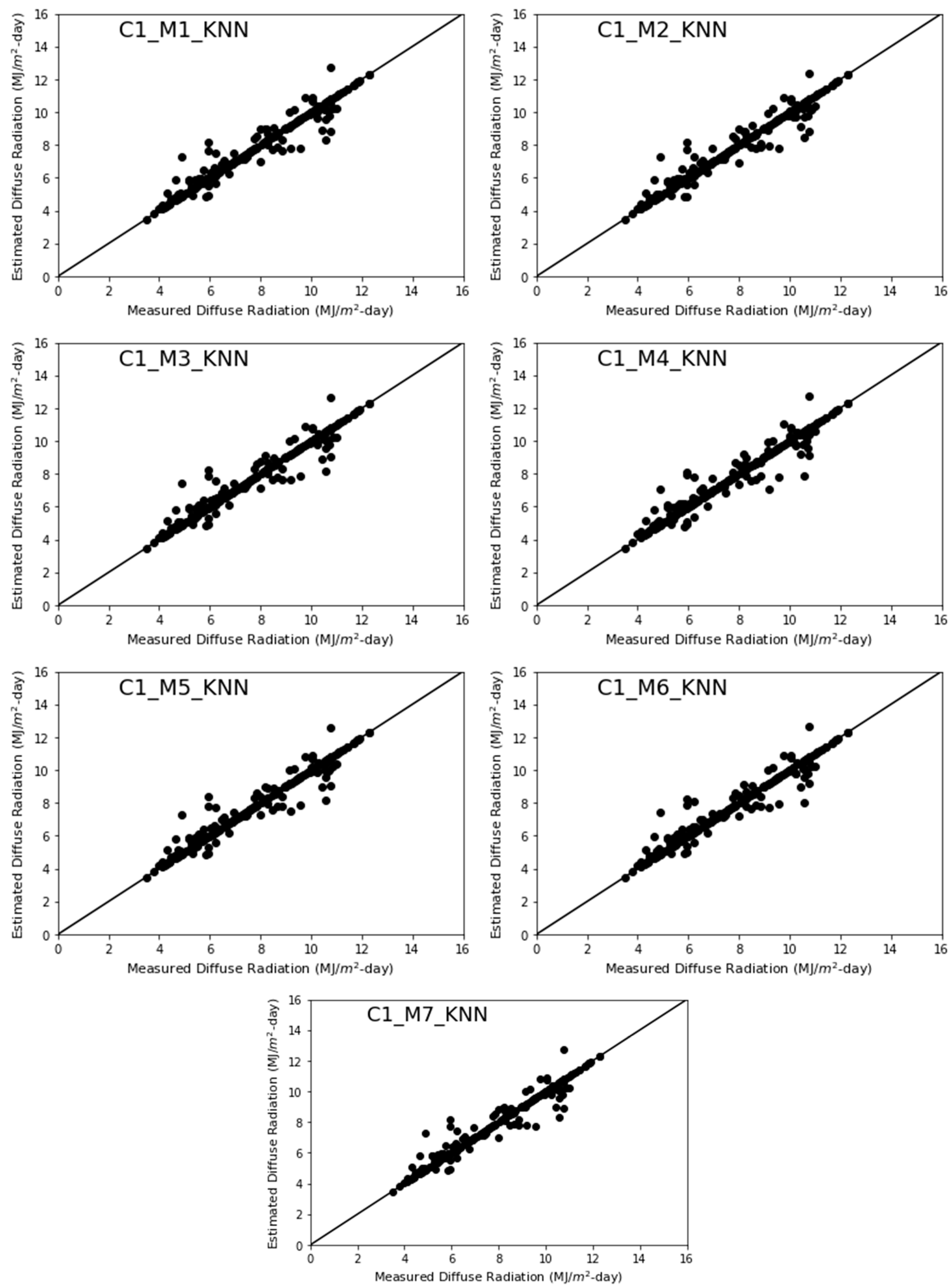
3.1. Category-1 Models (Diffuse Fraction)

In this, category seven models are proposed with two inputs having different function forms with a maximum order of two in each predictor. The various functional forms are as given below:

Form 1 ${\overline{D}}_f=f(\overline{K_t},\overline{\theta })$, Form 2 ${\overline{D}}_f=f(\overline{K_t},{\overline{K}}_t^2,\overline{\theta })$

Form 3 ${\overline{D}}_f=f(\overline{K_t},{\overline{K}}_t^2,\overline{\theta },{\overline{\theta }}_t^2)$, Form 4 ${\overline{D}}_f=f(\overline{K_t},\overline{\theta },{\overline{\theta }}_t^2)$

Form 5 ${\overline{D}}_f=f({\overline{K}}_t^2,{\overline{\theta }}_t^2)$, Form 6 ${\overline{D}}_f=f(\overline{K_t},{\overline{\theta }}_t^2)$, Form 7 ${\overline{D}}_f=f({\overline{K}}_t^2,\overline{\theta })$

Figure 2 and Figure 3 show the scatter plots of the estimated and measured DSR from category-1 models made with the KNN and RF ML techniques, respectively. The estimated DSR of all the developed models gives good correlations from the measured DSR. The coefficient of determination (R²) value lies in the range of 0.973–0.976 for KNN and 0.897–0.959 for RF.

In KNN models, the maximum value of R² is witnessed for Model 2, while the lowest R² is attained by Model 4, while in RF models, the maximum value of R² is witnessed for Model 3, while the lowest value of R² is for Model 5.

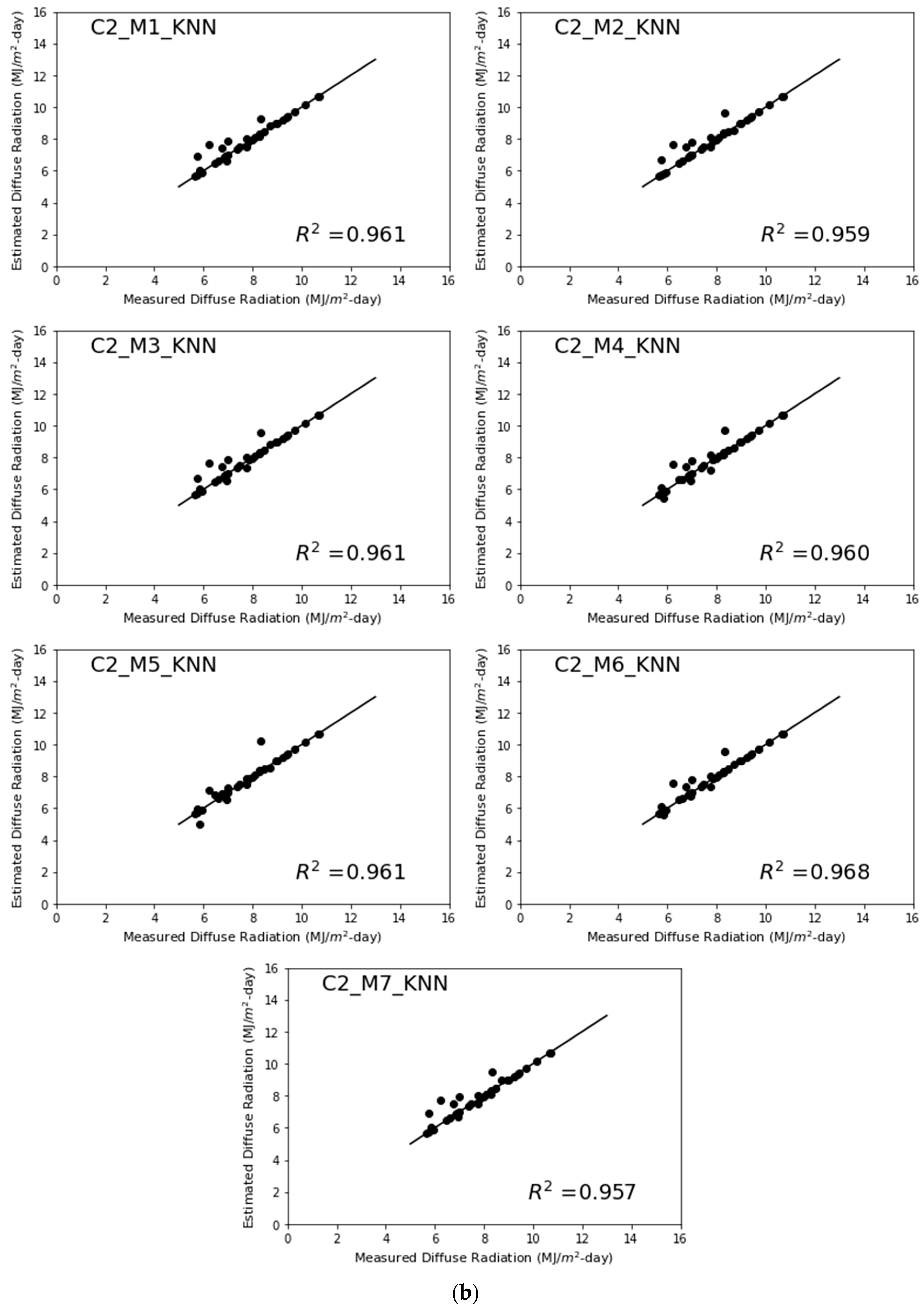
3.2. Category-2 Models (Diffusion Coefficient)

As a result of input predictors (such as sunlight ratio and clearness index), ML diffusion coefficient models are created. Seven further models are proposed in this category, all of which have comparable functional shapes to those in Category I.

Figure 4 and Figure 5 show the scatter diagrams of the predicted and measured DSR from category-2 models using KNN and RF ML techniques. All of the models that have been made show good correlations between the DSR they predict and the DSR they measure. The R² value for KNN is between 0.969 and 0.976, and the R² value for RF is between 0.935 and 0.958. In KNN models, Model 1 has the highest R² value and Model 5 has the lowest. In RF models, Model 3 has the highest R² value and Model 5 has the lowest.

3.3. Statistical Indicators

Table 3. Values of statistical indicators for the developed models.

Category 1 KNN
MODEL	MBE	RMS	MAPE	R2	U95
M1	0.0184	0.4829	2.8676	0.9751	4.2740
M2	0.0185	0.4710	2.8627	0.9763	4.2606
M3	0.0160	0.4888	2.8892	0.9744	4.2766
M4	0.0184	0.5018	3.0187	0.9731	4.2930
M5	0.0186	0.4850	2.9034	0.9748	4.2715
M6	0.0233	0.4935	2.9458	0.9740	4.2667
M7	0.0178	0.4798	2.8436	0.9754	4.2721
Category 1 RF
MODEL	MBE	RMS	MAPE	R2	U95
M1	0.0308	0.6356	5.9723	0.9568	4.1639
M2	0.0546	0.6411	6.0414	0.9561	4.1775
M3	0.0318	0.6199	5.9076	0.9592	4.1364
M4	0.0318	0.6210	5.9281	0.9591	4.1247
M5	0.1496	0.9825	9.6677	0.8977	4.5575
M6	0.0279	0.6334	6.0287	0.9575	4.1120
M7	0.0240	0.6241	5.8928	0.9587	4.1154
Category 2 KNN
MODEL	MBE	RMS	MAPE	R2	U95
M1	0.0287	0.4672	2.8298	0.9767	4.2701
M2	0.0263	0.4687	2.8714	0.9766	4.2605
M3	0.0291	0.4753	2.8856	0.9759	4.2832
M4	0.0324	0.4716	2.8664	0.9763	4.2704
M5	0.0249	0.5352	3.2885	0.9693	4.2474
M6	0.0333	0.4680	2.8668	0.9767	4.2644
M7	0.0297	0.4753	2.9052	0.9759	4.2884
Category 2 RF
MODEL	MBE	RMS	MAPE	R2	U95
M1	0.0577	0.6539	6.0563	0.9541	4.2479
M2	0.0427	0.6259	5.9015	0.9581	4.1959
M3	0.0366	0.6250	5.8853	0.9582	4.1768
M4	0.0350	0.6286	5.8954	0.9577	4.1827
M5	0.0542	0.7722	7.1921	0.9352	4.2726
M6	0.0469	0.6524	6.1011	0.9542	4.2592
M7	0.0535	0.6458	5.9996	0.9552	4.2343

displays the findings of statistical tests for both categories of models using the measures of Mean Bias Error (MBE), Root Mean Square Error (RMSE), Correlation coefficient (R²), Uncertainty at 95% (U95) and Mean Absolute Percentage Error (MAPE).

In Category 1 KNN models, Model 3 has a minimum value of 0.016 MJ/m²-day for MBE. The RMSE values lie in the range of 0.471–0.501 MJ/m²-day. The lowest value of RMSE is 0.471 MJ/m²-day for Model 2. The minimum value of MAPE is 2.862% for Model 2. The maximum value of R² is 0.976 for Model 2. The minimum value of U95 is 4.260 again for Model 2.

In Category 1 RF models, Model 7 has the lowest value of 0.024 MJ/m²-day for MBE. The lowest value of RMSE is 0.619 MJ/m²-day for Model 3. The MAPE values lie in the range of 5.892–9.667. The minimum value of MAPE is 5.892% for Model 7. The maximum value of R² is 0.959 for Model 3. The lowest value of U95 is 4.112 for Model 6.

In Category 2 KNN models, Model 5 has a minimum value of 0.024 MJ/m²-day for MBE. The RMSE values lie in the range of 0.468–0.535 MJ/m²-day. The minimum value of RMSE is 0.468 MJ/m²-day for Model 6. The lowest value of MAPE is 2.829% for Model 1. The maximum value of R² is 0.976 for Model 2. The minimum value of U-95 is 4.260 for Model 2.

Model 4 has the lowest value for MBE in Category 1 RF models, at 0.035 MJ/m²-day. The lowest value of RMSE for Model 3 is 0.625 MJ/m²-day. The MAPE values are between 5.887 and 7.192. Model 3 has a MAPE value of at least 5.885%. For Model 3, the most R² can be is 0.958. Model 6 has a U-95 value of 4.176, which is the lowest.

From the statistical parameters, it was observed that in general, KNN models performed well in comparison to RF models. Moreover, the effect of statistical indicators is not distinct and different statistical indicator values are in favour of different models; therefore, to remove this vagueness, the calculation of GPI is performed.

Figure 6 shows the GPI estimation of overall India consisting of different climatic zones. In category 1 KNN models, Model 2 ranked 1 (GPI = 1.393), followed by Model 7 (GPI = 0.682) and then Model 1. For category 1 RF models, Model 7 leads the 1st rank (GPI = 0.177), followed by Model 4 (0.099) and Model 3 (0.081). In category 2 KNN models, Model 2 is ranked 1st (GPI = 0.644), then Model 1 (GPI = 0.258) and then the rest of the models. In category 2 RF models, Model 3 is estimated 1^st rank, followed by Model 4 and then Model 2.

3.4. Comparison with Models Available in the Literature

The performance of the developed ML models is also compared with the models available in the literature to justify their development. Some well-established models are selected from the literature for the same according to their widespread application and similarity to the functional form of correlations. Here are the models that were chosen for both groups:

Jamil et al. Model 1 [59]

$${\overline{D}}_f=2.071-0.9142\overline{K_t}-2.6184\overline{\theta }+1.5116{\overline{\theta }}^2$$

El-Sebaii et al. Model [26]

$${\overline{D}}_f=4.609-6.318\overline{K_t}-0.0474\overline{\theta }$$

Jamil et al. Model 2 [64]

$${\overline{D}}_c=0.3960-0.9827\overline{K_t}-0.9510{\overline{K_t}}^2-0.9104\overline{\theta }+0.4658{\overline{\theta }}^2$$

Li et al. Model [38]

$${\overline{D}}_c=-0.0493+1.414\overline{K_t}-1.95{\overline{K_t}}^2-0.0306\overline{\theta }+0.1269{\overline{\theta }}^2$$

The scatter plots of the models suggested by earlier investigations are displayed in Figure 7. The scatter plots demonstrate that the generated ML models outperform the models found in the literature in terms of estimating DSR. The projected values are far from the measured data, and the coefficient of determination values are also significantly lower. This justifies the creation of ML models.

3.5. Application of Developed ML Models under Various Climatic Zones

The ML models developed in both categories have been employed to predict DSR for five climatic zones of India. As the performance of KNN models is better in comparison to RF Models, we used KNN models for application. The scatter diagrams of the predicted and measured values of DSR are shown in Figure 8, Figure 9, Figure 10, Figure 11 and Figure 12.

Category 1 and Category 2 models are presented in Figure 8, Figure 9, Figure 10, Figure 11 and Figure 12 for each climatic zone, along with values of the correlation coefficient on each graph. It can be seen that the ML model gives very good predictions with excellent correlation values for all the climatic zones. Further, it can be seen that within each category, the difference in R² values is almost negligible. That means any functional form can be used with great accuracy. Moreover, Category II type models provide better R² values in comparison to Category I models.

Table 4. Statistical indicator values for Category-1 ML models for different climatic zone.

Statistical Indicators	M1	M2	M3	M4	M5	M6	M7
Subtropical Humid Climate
MBE	0.0153	0.04958	0.04982	0.03421	0.11709	0.03594	0.01333
RMS	0.53641	0.47977	0.47536	0.4892	0.80273	0.48119	0.54086
MAPE	3.64847	3.25416	3.42663	3.14276	4.85124	3.15851	3.67562
R2	0.9643	0.97163	0.97233	0.97015	0.91944	0.97119	0.96349
U95	4.0609	4.0166	4.04438	3.97301	4.07976	3.98406	4.03424
Tropical Wet and Dry Climate
MBE	−0.0198	−0.0045	0.18863	−0.025	−0.1265	−0.0242	−0.0094
RMS	0.43637	0.3967	0.52074	0.5125	0.70671	0.53061	0.45662
MAPE	2.82463	2.69795	3.49768	3.47452	4.81819	3.52993	3.01713
R2	0.97825	0.98195	0.93676	0.97128	0.9501	0.96896	0.97605
U95	4.16592	4.11663	2.718	4.33419	4.5813	4.32611	4.14535
Tropical Wet Climate
MBE	0.18451	0.19367	0.18863	0.15124	0.0903	0.15119	0.19047
RMS	0.5119	0.54096	0.52074	0.49994	0.50535	0.47964	0.52481
MAPE	3.45867	3.69023	3.49768	3.33996	3.36727	3.12059	3.47919
R2	0.93887	0.93129	0.93676	0.93908	0.93349	0.94458	0.93577
U95	2.71396	2.72576	2.718	2.71985	2.70542	2.71585	2.71658
Semi-Arid Climate
MBE	−0.0165	0.01626	−0.0182	−0.0392	−0.0193	−0.0215	−0.0124
RMS	0.35813	0.38162	0.3685	0.37733	0.48067	0.38381	0.36875
MAPE	2.54478	2.83289	2.51074	2.50675	3.50534	2.67787	2.66804
R2	0.99007	0.98874	0.98949	0.98914	0.98232	0.98863	0.98945
U95	5.00651	4.94223	5.01482	5.04959	5.10824	5.02953	4.9945
Arid climate
MBE	−0.0984	−0.1125	−0.11	−0.1132	−0.026	−0.1045	−0.1106
RMS	0.5031	0.50485	0.53621	0.4898	0.81585	0.49569	0.54327
MAPE	3.40123	3.17594	3.32376	3.32639	4.55863	3.44428	3.4506
R2	0.98118	0.98129	0.9787	0.98243	0.94759	0.98182	0.97811
U95	4.96069	4.95572	4.95043	4.98537	5.01664	4.99313	4.95219

and

Table 5. Statistical indicator values for Category-2 ML models for different climatic zone.

Statistical Indicators	M1	M2	M3	M4	M5	M6	M7
Subtropical Humid Climate
MBE	0.08049	0.08425	0.09688	0.09908	0.12637	0.10152	0.08551
RMS	0.36514	0.35239	0.36849	0.38135	0.52135	0.39456	0.36629
MAPE	2.47727	2.37231	2.55948	2.52881	3.24061	2.70167	2.48456
R2	0.9842	0.98547	0.98431	0.98319	0.96787	0.98187	0.98421
U95	3.93184	3.90786	3.90678	3.89485	3.93957	3.95246	3.92453
Tropical Wet Climate
MBE	−0.0232	−0.0402	−0.0347	−0.0426	−0.1222	−0.0339	−0.0156
RMS	0.43388	0.38702	0.43687	0.45727	0.52158	0.47781	0.4500
MAPE	2.79622	2.49522	2.68675	3.04722	3.74846	3.14585	2.92803
R2	0.97845	0.98302	0.97829	0.97655	0.97092	0.9743	0.97674
U95	4.14146	4.09406	4.16652	4.22508	4.25516	4.23394	4.12539
Tropical Wet Climate
MBE	0.13974	0.14864	0.13456	0.09937	0.06695	0.10583	0.15494
RMS	0.40456	0.41659	0.40348	0.40308	0.40135	0.36299	0.43201
MAPE	2.63089	2.52613	2.61344	2.66005	2.25833	2.22035	2.80961
R2	0.9618	0.9598	0.96163	0.96037	0.9615	0.96833	0.95676
U95	2.70975	2.7432	2.74135	2.83408	2.93013	2.77822	2.74244
Semi-Arid Climate
MBE	0.00831	0.04793	−0.0039	−0.0209	−0.036	−0.0096	−0.015
RMS	0.36957	0.39005	0.37081	0.35845	0.39496	0.3526	0.35598
MAPE	2.74369	2.88485	2.72468	2.50349	3.04694	2.49646	2.60209
R2	0.98941	0.98842	0.98937	0.99018	0.98838	0.99044	0.99037
U95	5.01198	4.93082	5.03641	5.06411	5.12757	5.05057	5.08208
Arid climate
MBE	−0.0774	−0.0872	−0.0715	−0.0593	−0.034	−0.0598	−0.0868
RMS	0.45428	0.44603	0.45831	0.47786	0.55422	0.47479	0.44612
MAPE	2.84947	2.72332	2.83975	2.97329	3.21218	2.94535	2.75219
R2	0.98451	0.98521	0.98415	0.98259	0.97623	0.98282	0.9852
U95	5.02221	5.02634	5.01465	5.0002	4.98917	5.00052	5.02146

display the results of statistical indicator analysis for both category models for five climatic zones. From Table 4 and Table 5, overestimation is observed as MBE values are positive for subtropical humid climate and tropical wet climate, whereas an underestimation in the prediction of DSR values has been witnessed for tropical wet and dry climate, arid climate and semi-arid climate as the MBE values are negative. For semi-arid climate, in category 1 models, Model 1 and Model 2 show overestimation while the rest of the models show underestimation. The best models in category 1 with respect to MBE are Model 5, Model 2, Model 5, Model 7 and Model 5 for SHC, TWDC, TWC, SARC and ARC, respectively. In category 2, the best models with respect to MBE are Model 1, Model 7, Model 5, Model 3 and Model 5 for SHC, TWDC, TWC, SARC and ARC, respectively.

The RMSE values are witnessed to be considerably small for all the climatic zones representing good estimation. In category 1, the lowest RMSE values are witnessed as 0.481, 0.396, 0.479, 0.358 and 0.489 MJ/m²-day, respectively, for SHC (Model 6), TWDC (Model 2), TWC (Model 6), SARC (Model 1) and ARC (Model 4). The minimum value of RMSE in category 2 are 0.352, 0.387, 0.362, 0.352 and 0.446 MJ/m²-day for SHC (Model 2), TWDC (Model 2), TWC (Model 6), SARC (Model 6) and ARC (Model 2), respectively.

MAPE values are lowest for Model 4 (3.142), Model 2 (2.697), Model 6 (3.120), Model 4 (2.506) and Model 2 (3.175), respectively, for SHC, TWDC, TWC, SARC and ARC in category 1. In category 2, MAPE values are least for Model 2 (2.372), Model 2 (2.495), Model 6 (2.220), Model 6 (2.496) and Model 2 (2.723) for SHC, TWDC, TWC, SARC and ARC, respectively.

The top-performing models in terms of R² in category 1 are Model 3, Model 2, Model 6, Model 1 and Model 2, while in category 2 are Model 2, Model 2, Model 6, Model 6 and Model 2 for SHC, TWDC, TWC, SARC and ARC, respectively.

In category 1, the lowest values of U95 are observed as 3.973, 2.718, 2.705, 4.942 and 4.950 MJ/m²-day, respectively, for SHC (Model 4), TWDC (Model 3), TWC (Model 5), SARC (Model 4) and ARC (Model 3). The minimum values of U95 in category 2 are 3.906, 4.094, 2.709, 4.930 and 4.989 MJ/m²-day for SHC (Model 6), TWDC (Model 2), TWC (Model 1), SARC (Model 1) and ARC (Model 5), respectively. So, it is clear that the individual values of statistical indicators are not enough to choose the best model, since they support different models. So, GPI and the parallel ranking system need to be used to expand statistical analysis.

Figure 13 shows the GPI estimation of all the climatic zones. For subtropical humid climate, in category 1, Model 4 (GPI = 0.754) is best, while Model 2 (GPI = 0.912) ranked 1 in category 2. For the tropical wet and dry climatic region, Model 2 leads the 1st rank in both categories. Model 6 is the best model in both categories for tropical wet climate. For the semi-arid climatic region, in category 1, Model 4 is best, while Model 6 ranked 1 in category 2. For the arid climatic region, Model 2 is ranked 1 in category 1, while Model 7 is best for category 2.

Table 6. Overall ranking of ML models under different climatic zones.

Rank	SHC	TWD	TW	SAR	AR
1	M2C2	M2C2	M6C2	M2C1	M2C1
2	M1C2	M2C1	M1C2	M1 C1	M3C1
3	M7C2	M3C2	M3C2	M3C1	M7C1
4	M4C2	M1C2	M5C2	M6C2	M1 C1
5	M3C2	M1 C1	M2C2	M4C1	M4C1
6	M6C2	M7C2	M4C2	M4C2	M7C2
7	M4C1	M4C2	M7C2	M7C1	M6C1
8	M6C1	M7C1	M6C1	M7C2	M2C2
9	M2C1	M6C2	M5C1	M6C1	M3C2
10	M3C1	M5C2	M4C1	M3C2	M1C2
11	M7C1	M4C1	M1 C1	M1C2	M4C2
12	M1 C1	M6C1	M3C1	M2C2	M6C2
13	M5C2	M3C1	M7C1	M5C2	M5C2
14	M5C1	M5C1	M2C1	M5C1	M5C1

shows the overall ranking of all ML models proposed in both categories. Model 2 (Cat-2) for SHC, Model 2 (Cat-2) for TWDC, Model 6 (Cat-2) for TWC, Model 2 (Cat-1) for SARC and Model 2 (Cat-1) for ARC, all come to Rank first.

4. Conclusions

In the present work, ML techniques are used to predict DSR for Indian climatic zones with two input predictors having different functional forms with a maximum order of two in each predictor. The results show that the ML model gives better predictions for most of the climate zones in comparison to empirical models. It is concluded that the ML models perform splendidly for the five climatic zones for both categories. However, based on overall GPI, category 2 models overtake category 1 models. This work would be valuable for climatic regions within India as well as outside where the constraint of solar radiation apparatus curbs the prediction of DSR under different climatic zones.

In category 1 models, Model 4 performs for SHC with values statistical indicators (MBE, RMS, MAPE, R², U95) of 0.0342, 0.489, 3.142, 0.970 and 3.973, respectively. Model 2 shows top performance again with values of statistical indicators as −0.0045, 0.3967, 2.69795, 0.98195 and 4.11663, respectively, at TWDC. For TWC, Model 6 performs well with statistical indicator values of 0.15119, 0.47964, 3.12059, 0.94458 and 2.71585, respectively. Model 4 again performs well with values of statistical indicators of −0.0392, 0.37733, 2.50675, 0.98914 and 5.04959, respectively, at SARC. Model 2 again performs well for ARC with values of statistical indicators values as −0.1125, 0.50485, 3.17594, 0.98129 and 4.95572, respectively.

In category 2, Model 2 perform well for SHC and TWDC while Model 6 for TWC and SARC. For ARC, Model 7 shows top performance. Considering all the developed models together, the results indicate that Model 2 (C2) is best for SHC and TWDC, while Model 2 (C1) gives top performance for ARC and SARC and Model 6 (C2) is best for TWC.

5. Limitations of the Present Work

The accuracy of ML methods depends on the quality of the training data. So, if training data are not sufficient or incorrect then predictions using ML methods may be misleading. Another limitation is the proper selection of hyper parameters for training ML model. In a case where hyper parameters are not selected properly, inaccurate predictions may be obtained.

References

1. Voyant, C.; Notton, G.; Kalogirou, S.; Nivet, M.-L.; Paoli, C.; Motte, F.; Fouilloy, A. Machine learning methods for solar radiation forecasting: A review. Renew Energy 2017, 105, 569–582. [Google Scholar] [CrossRef]
2. Ramachandra, T.V.; Jain, R.; Krishnadas, G. Hotspots of solar potential in India. Renew. Sustain. Energy Rev. 2011, 15, 3178–3186. [Google Scholar] [CrossRef]
3. Kapoor, K.; Pandey, K.K.; Jain, A.; Nandan, A. Evolution of solar energy in India: A review. Renew. Sustain. Energy Rev. 2014, 40, 475–487. [Google Scholar] [CrossRef]
4. Pandey, S.; Singh, V.S.; Gangwar, N.P.; Vijayvergia, M.; Prakash, C.; Pandey, D.N. Determinants of success for promoting solar energy in Rajasthan, India. Renew. Sustain. Energy Rev. 2012, 16, 3593–3598. [Google Scholar] [CrossRef]
5. Salmi, M.; Chegaar, M.; Mialhe, P. A Collection of Models for the Estimation of Global Solar Radiation in Algeria. Energy Sources Part B Econ. Plan. Policy 2011, 6, 187–191. [Google Scholar] [CrossRef]
6. Rehman, S. Solar radiation over Saudi Arabia and comparisons with empirical models. Energy 1998, 23, 1077–1082. [Google Scholar] [CrossRef]
7. Rehman, S.; Ghori, S.G. Spatial estimation of global solar radiation using geostatistics. Renew. Energy 2000, 21, 583–605. [Google Scholar] [CrossRef]
8. Alqaed, S.; Mustafa, J.; Almehmadi, F.A. Design and energy requirements of a photovoltaic-thermal powered water de-salination plant for the middle east. Int. J. Environ. Res. Public Health 2021, 18, 1001. [Google Scholar] [CrossRef]
9. Mustafa, J.; Alqaed, S.; Almehmadi, F.A.; Jamil, B. Development and comparison of parametric models to predict global solar radiation: A case study for the southern region of Saudi Arabia. J. Therm. Anal. Calorim. 2022, 147, 9559–9589. [Google Scholar] [CrossRef]
10. Alqaed, S.; Mustafa, J.; Sharifpur, M.; Alharthi, M.A. Numerical simulation and artificial neural network modeling of exergy and energy of parabolic trough solar collectors equipped with innovative turbulators containing hybrid nanofluids. J. Therm. Anal. Calorim. 2022, 1–16. [Google Scholar] [CrossRef]
11. Jamil, B.; Akhtar, N. Statistical Analysis of Short-Term Solar Radiation Data over Aligarh (India). In Progress in Clean Energy; Volume 2: Novel Systems and Applications; Springer International Publishing: Cham, Switzerland, 2015; Volume 2, pp. 937–948. [Google Scholar] [CrossRef]
12. Rehman, S.; Mohandes, M. Artificial neural network estimation of global solar radiation using air temperature and relative humidity. Energy Policy 2008, 36, 571–576. [Google Scholar] [CrossRef] [Green Version]
13. Zeng, J.; Qiao, W. Short-term solar power prediction using a support vector machine. Renew. Energy 2013, 52, 118–127. [Google Scholar] [CrossRef]
14. McCormick, P.; Suehrcke, H. Diffuse fraction correlations. Sol. Energy 1991, 47, 311–312. [Google Scholar] [CrossRef]
15. Angstrom, A. Solar and terrestrial radiation. Report to the international commission for solar research on actinometric investigations of solar and atmospheric radiation. Q. J. R. Meteorol. Soc. 1924, 50, 121–126. [Google Scholar] [CrossRef]
16. Iqbal, M. Prediction of hourly diffuse solar radiation from measured hourly global radiation on a horizontal surface. Sol. Energy 1980, 24, 491–503. [Google Scholar] [CrossRef]
17. Liu, B.Y.H.; Jordan, R.C. The interrelationship and characteristic distribution of direct, diffuse and total solar radiation. Sol. Energy 1960, 4, 1–19. [Google Scholar] [CrossRef]
18. Karakoti, I.; Das, P.K.; Bandyopadhyay, B. Diffuse radiation models for Indian climatic conditions. Int. J. Ambient. Energy 2012, 33, 75–86. [Google Scholar] [CrossRef]
19. Jafari, S.; Javaran, E.J. An Optimum Slope Angle for Solar Collector Systems in Kerman Using a New Model for Diffuse Solar Radiation. Energy Sources, Part A: Recover. Util. Environ. Eff. 2012, 34, 799–809. [Google Scholar] [CrossRef]
20. Al-Mohamad, A. Global, direct and diffuse solar-radiation in Syria. Appl. Energy 2004, 79, 191–200. [Google Scholar] [CrossRef]
21. Noorian, A.M.; Moradi, I.; Kamali, G.A. Evaluation of 12 models to estimate hourly diffuse irradiation on inclined surfaces. Renew. Energy 2008, 33, 1406–1412. [Google Scholar] [CrossRef]
22. Diez-Mediavilla, M.; de Miguel, A.; Bilbao, J. Measurement and comparison of diffuse solar irradiance models on inclined surfaces in Valladolid (Spain). Energy Convers. Manag. 2005, 46, 2075–2092. [Google Scholar] [CrossRef]
23. Tarhan, S.; Sari, A. Model selection for global and diffuse radiation over the Central Black Sea (CBS) region of Turkey. Energy Convers. Manag. 2005, 46, 605–613. [Google Scholar] [CrossRef]
24. Aras, H.; Balli, O.; Hepbasli, A. Estimating the horizontal diffuse solar radiation over the Central Anatolia Region of Turkey. Energy Convers. Manag. 2006, 47, 2240–2249. [Google Scholar] [CrossRef]
25. Boland, J.; Scott, L.; Luther, M. Modelling the diffuse fraction of global solar radiation on a horizontal surface. Environmetrics 2001, 12, 103–116. [Google Scholar] [CrossRef]
26. El-Sebaii, A.; Al-Hazmi, F.; Al-Ghamdi, A.; Yaghmour, S. Global, direct and diffuse solar radiation on horizontal and tilted surfaces in Jeddah, Saudi Arabia. Appl. Energy 2010, 87, 568–576. [Google Scholar] [CrossRef]
27. Iqbal, M. A study of Canadian diffuse and total solar radiation data—II Monthly average hourly horizontal radiation. Sol. Energy 1979, 22, 87–90. [Google Scholar] [CrossRef]
28. Boland, J.; Ridley, B.; Brown, B. Models of diffuse solar radiation. Renew. Energy 2008, 33, 575–584. [Google Scholar] [CrossRef]
29. Gopinathan, K. Empirical correlations for diffuse solar irradiation. Sol. Energy 1988, 40, 369–370. [Google Scholar] [CrossRef]
30. El-Sebaii, A.; Trabea, A. Estimation of horizontal diffuse solar radiation in Egypt. Energy Convers. Manag. 2003, 44, 2471–2482. [Google Scholar] [CrossRef]
31. Jiang, Y. Estimation of monthly mean daily diffuse radiation in China. Appl. Energy 2009, 86, 1458–1464. [Google Scholar] [CrossRef]
32. Wattan, R.; Janjai, S. An investigation of the performance of 14 models for estimating hourly diffuse irradiation on inclined surfaces at tropical sites. Renew. Energy 2016, 93, 667–674. [Google Scholar] [CrossRef]
33. Ulgen, K.; Hepbasli, A. Diffuse solar radiation estimation models for Turkey’s big cities. Energy Convers. Manag. 2009, 50, 149–156. [Google Scholar] [CrossRef]
34. Kaygusuz, K. The Comparison of Measured and Calculated Solar Radiations in Trabzon, Turkey. Energy Sources 1999, 21, 347–353. [Google Scholar] [CrossRef]
35. Bakirci, K. The Calculation of Diffuse Radiation on a Horizontal Surface for Solar Energy Applications. Energy Sources Part A Recover. Util. Environ. Eff. 2012, 34, 887–898. [Google Scholar] [CrossRef]
36. Paulescu, E.; Blaga, R. Regression models for hourly diffuse solar radiation. Sol. Energy 2016, 125, 111–124. [Google Scholar] [CrossRef]
37. Magarreiro, C.; Brito, M.; Soares, P. Assessment of diffuse radiation models for cloudy atmospheric conditions in the Azores region. Sol. Energy 2014, 108, 538–547. [Google Scholar] [CrossRef]
38. Li, H.; Ma, W.; Wang, X.; Lian, Y. Estimating monthly average daily diffuse solar radiation with multiple predictors: A case study. Renew. Energy 2011, 36, 1944–1948. [Google Scholar] [CrossRef]
39. Safaripour, M.H.; Mehrabian, M.A. Predicting the direct, diffuse, and global solar radiation on a horizontal surface and comparing with real data. Heat Mass Transf. 2011, 47, 1537–1551. [Google Scholar] [CrossRef]
40. Filho, E.P.M.; Oliveira, A.P.; Vita, W.A.; Mesquita, F.L.; Codato, G.; Escobedo, J.F.; Cassol, M.; França, J.R.A. Global, diffuse and direct solar radiation at the surface in the city of Rio de Janeiro: Observational characterization and empirical modeling. Renew. Energy 2016, 91, 64–74. [Google Scholar] [CrossRef]
41. Despotovic, M.; Nedic, V.; Despotovic, D.; Cvetanovic, S. Evaluation of empirical models for predicting monthly mean horizontal diffuse solar radiation. Renew. Sustain. Energy Rev. 2016, 56, 246–260. [Google Scholar] [CrossRef]
42. Soares, J.; Oliveira, A.P.; Božnar, M.Z.; Mlakar, P.; Escobedo, J.F.; Machado, A.J. Modeling hourly diffuse solar-radiation in the city of São Paulo using a neural-network technique. Appl. Energy 2004, 79, 201–214. [Google Scholar] [CrossRef]
43. Şenkal, O.; Kuleli, T. Estimation of solar radiation over Turkey using artificial neural network and satellite data. Appl. Energy 2009, 86, 1222–1228. [Google Scholar] [CrossRef]
44. Khatib, T.; Mohamed, A.; Mahmoud, M.; Sopian, K. Modeling of Daily Solar Energy on a Horizontal Surface for Five Main Sites in Malaysia. Int. J. Green Energy 2011, 8, 795–819. [Google Scholar] [CrossRef]
45. Rehman, S.; Mohandes, M. Estimation of Diffuse Fraction of Global Solar Radiation Using Artificial Neural Networks. Energy Sources Part A Recover. Util. Environ. Eff. 2009, 31, 974–984. [Google Scholar] [CrossRef]
46. Mellit, A.; Kalogirou, S.A. Artificial intelligence techniques for photovoltaic applications: A review. Prog. Energy Combust. Sci. 2008, 34, 574–632. [Google Scholar] [CrossRef]
47. Mubiru, J. Predicting total solar irradiation values using artificial neural networks. Renew. Energy 2008, 33, 2329–2332. [Google Scholar] [CrossRef]
48. Salcedo-Sanz, S.; Casanova-Mateo, C.; Pastor-Sánchez, A.; Gallo-Marazuela, D.; Labajo-Salazar, A.; Portilla-Figueras, A. Direct Solar Radiation Prediction Based on Soft-Computing Algorithms Including Novel Predictive Atmospheric Variables. In Lecture Notes in Computer Science (Including Subseries Lecture Notes in Artificial Intelligence and Lecture Notes in Bioinformatics); Springer: Berlin, Germany, 2013; Volume 8206, pp. 318–325. [Google Scholar]
49. Belaid, S.; Mellit, A. Prediction of daily and mean monthly global solar radiation using support vector machine in an arid climate. Energy Convers. Manag. 2016, 118, 105–118. [Google Scholar] [CrossRef]
50. Benghanem, M.; Mellit, A. Radial Basis Function Network-based prediction of global solar radiation data: Application for sizing of a stand-alone photovoltaic system at Al-Madinah, Saudi Arabia. Energy 2010, 35, 3751–3762. [Google Scholar] [CrossRef]
51. Aybar-Ruiz, A.; Jiménez-Fernández, S.; Cornejo-Bueno, L.; Casanova-Mateo, C.; Sanz-Justo, J.; Salvador-González, P.; Salcedo-Sanz, S. A novel Grouping Genetic Algorithm–Extreme Learning Machine approach for global solar radiation prediction from numerical weather models inputs. Sol. Energy 2016, 132, 129–142. [Google Scholar] [CrossRef]
52. Salcedo-Sanz, S.; Casanova-Mateo, C.; Munoz-Mari, J.; Camps-Valls, G. Prediction of Daily Global Solar Irradiation Using Temporal Gaussian Processes. IEEE Geosci. Remote Sens. Lett. 2014, 11, 1936–1940. [Google Scholar] [CrossRef]
53. Dong, H.; Yang, L.; Zhang, S.; Li, Y. An Improved Prediction Approach on Solar Irradiance of Photovoltaic Power Station. TELKOMNIKA Indones. J. Electr. Eng. 2013, 12, 1720–1726. [Google Scholar] [CrossRef]
54. Ibrahim, I.A.; Khatib, T. A novel hybrid model for hourly global solar radiation prediction using random forests technique and firefly algorithm. Energy Convers. Manag. 2017, 138, 413–425. [Google Scholar] [CrossRef]
55. Salcedo-Sanz, S.; Casanova-Mateo, C.; Pastor-Sánchez, A.; Sánchez-Girón, M. Daily global solar radiation prediction based on a hybrid Coral Reefs Optimization–Extreme Learning Machine approach. Sol. Energy 2014, 105, 91–98. [Google Scholar] [CrossRef]
56. Mustafa, J.; Alqaed, S.; Aybar, H.; Husain, S. Investigation of the effect of twisted tape turbulators on thermal-hydraulic behavior of parabolic solar collector with polymer hybrid nanofluid and exergy analysis using numerical method and ANN. Eng. Anal. Bound. Elem. 2022, 144, 81–93. [Google Scholar] [CrossRef]
57. Mustafa, J.; Alqaed, S.; Sharifpur, M.; Alharthi, M.A. Combined simulation of molecular dynamics and computational fluid dynamics to predict the properties of a nanofluid flowing inside a micro-heatsink by modeling a radiator with holes on its fins. J. Mol. Liq. 2022, 362, 119727. [Google Scholar] [CrossRef]
58. Mustafa, J.; Alqaed, S.; Sharifpur, M. Numerical study on performance of double-fluid parabolic trough solar collector occupied with hybrid non-Newtonian nanofluids: Investigation of effects of helical absorber tube using deep learning. Eng. Anal. Bound. Elem. 2022, 140, 562–580. [Google Scholar] [CrossRef]
59. Modi, V.; Sukhatme, S. Estimation of daily total and diffuse insolation in India from weather data. Sol. Energy 1979, 22, 407–411. [Google Scholar] [CrossRef]
60. Hawas, M.; Muneer, T. Study of diffuse and global radiation characteristics in India. Energy Convers. Manag. 1984, 24, 143–149. [Google Scholar] [CrossRef]
61. Veeran, P.; Kumar, S. Diffuse radiation on a horizontal surfaces at Madras. Renew. Energy 1993, 3, 931–934. [Google Scholar] [CrossRef]
62. Parishwad, G.; Bhardwaj, R.; Nema, V. Estimation of hourly solar radiation for India. Renew. Energy 1997, 12, 303–313. [Google Scholar] [CrossRef]
63. Jamil, B.; Siddiqui, A.T. Generalized models for estimation of diffuse solar radiation based on clearness index and sunshine duration in India: Applicability under different climatic zones. J. Atmos. Sol.-Terr. Phys. 2017, 157–158, 16–34. [Google Scholar] [CrossRef]
64. Jamil, B.; Akhtar, N. Comparison of empirical models to estimate monthly mean diffuse solar radiation from measured data: Case study for humid-subtropical climatic region of India. Renew. Sustain. Energy Rev. 2017, 77, 1326–1342. [Google Scholar] [CrossRef]
65. Mustafa, J.; Husain, S.; Khan, U.A.; Akhtar, M. Prediction of diffuse solar radiation using machine learning models based on sunshine period and sky-clearness index for the humid-subtropical climate of India. Environ. Prog. Sustain. Energy 2022. [Google Scholar] [CrossRef]
66. Kottek, M.; Grieser, J.; Beck, C.; Rudolf, B.; Rubel, F. World map of the Köppen-Geiger climate classification updated. Meteorol. Z. 2006, 15, 259–263. [Google Scholar] [CrossRef]
67. Tyagi, A.P. Solar Radiant Energy Over India; India Meteorological Department Ministry of Earth Sciences: New Delhi, India, 2009. Available online: https://www.imdpune.gov.in/library/public/Solar%20Radiant%20Energy%20Over%20India.pdf (accessed on 10 September 2022).
68. Klein, S. Calculation of monthly average insolation on tilted surfaces. Sol. Energy 1977, 19, 325–329. [Google Scholar] [CrossRef] [Green Version]
69. Khorasanizadeh, H.; Mohammadi, K.; Goudarzi, N. Prediction of horizontal diffuse solar radiation using clearness index based empirical models; A case study. Int. J. Hydrogen Energy 2016, 41, 21888–21898. [Google Scholar] [CrossRef]
70. Pedro, H.T.; Coimbra, C.F. Nearest-neighbor methodology for prediction of intra-hour global horizontal and direct normal irradiances. Renew. Energy 2015, 80, 770–782. [Google Scholar] [CrossRef]
71. Huang, J.; Troccoli, A.; Coppin, P. An analytical comparison of four approaches to modelling the daily variability of solar irradiance using meteorological records. Renew. Energy 2014, 72, 195–202. [Google Scholar] [CrossRef]
72. Alfadda, A.; Rahman, S.; Pipattanasomporn, M. Solar irradiance forecast using aerosols measurements: A data driven approach. Sol. Energy 2018, 170, 924–939. [Google Scholar] [CrossRef]
73. Breiman, L. Random forests. Mach. Learn. 2001, 45, 5–32. [Google Scholar] [CrossRef] [Green Version]
74. Feng, Y.; Cui, N.; Zhang, Q.; Zhao, L.; Gong, D. Comparison of artificial intelligence and empirical models for estimation of daily diffuse solar radiation in North China Plain. Int. J. Hydrogen Energy 2017, 42, 14418–14428. [Google Scholar] [CrossRef]
75. Despotovic, M.; Nedic, V.; Despotovic, D.; Cvetanovic, S. Review and statistical analysis of different global solar radiation sunshine models. Renew. Sustain. Energy Rev. 2015, 52, 1869–1880. [Google Scholar] [CrossRef]
Figure 1. Indian meteorological stations, 21 of which are geographically located.
Energies 15 07851 g001
Figure 2. Plot depicting predicted and measured DSR from KNN ML models (Category 1).
Energies 15 07851 g002
Figure 3. Plot depicting predicted and measured DSR from RF ML models (Category 1).
Energies 15 07851 g003
Figure 4. Plot depicting predicted and measured DSR from KNN ML models (Category 2).
Energies 15 07851 g004aEnergies 15 07851 g004b
Figure 5. Plot depicting predicted and measured DSR from RF ML models (Category 2).
Energies 15 07851 g005aEnergies 15 07851 g005b
Figure 6. Global performance indicators of both groups of machine learning models for the Indian Climate.
Energies 15 07851 g006
Figure 7. Plot depicting predicted and measured DSR from models selected from the literature.
Energies 15 07851 g007
Figure 8. (a) Plot depicting predicted and measured DSR for subtropical humid climate (Category 1). (b) Plot depicting predicted and measured DSR for subtropical humid climate (Category 2).
Energies 15 07851 g008aEnergies 15 07851 g008b
Figure 9. (a) Plot depicting predicted and measured DSR tropical wet and dry climate (Category I). (b) Plot depicting predicted and measured DSR tropical wet and dry climate (Category 2).
Energies 15 07851 g009aEnergies 15 07851 g009b
Figure 10. (a) Plot depicting predicted and measured DSR tropical wet climate (Category I). (b) Plot depicting predicted and measured DSR tropical wet climate (Category 2).
Energies 15 07851 g010aEnergies 15 07851 g010b
Figure 11. (a) Plot depicting predicted and measured DSR Semi-arid climate (Category I). (b) Plot depicting predicted and measured DSR Semi-arid climate (Category 2).
Energies 15 07851 g011aEnergies 15 07851 g011b
Figure 12. (a) Plot depicting predicted and measured DSR Arid climate (Category I). (b) Plot depicting predicted and measured DSR Arid climate (Category I).
Energies 15 07851 g012aEnergies 15 07851 g012b
Figure 13. Global performance indicator of machine learning models at the five climatic zones of India from both categories.
Energies 15 07851 g013aEnergies 15 07851 g013b