1. Introduction
Current trends in energy research lean toward fuel consumption and carbon dioxide emission reduction [
1,
2]. These aims fall under broad titles in research such as renewable energy and energy management systems. Engineering systems and applications often include processes and components that require and consume significant energy; this makes energy management one of the primordial solutions to achieve a suitable setup in terms of performance, consumption, and emission [
3,
4]. The automotive domain is a prime example of a system that requires energy management, particularly due to the huge amounts of energy lost by heat through the exhaust and water-cooling systems [
5,
6]. Therefore, the optimization of vehicle cooling modules is directly related to energy consumption and carbon dioxide emission reduction goals. Moreover, with the optimization of the cooling system operation, acceptable magnitude orders of fuel consumption and carbon dioxide emission reductions can be obtained.
Cooling modules of vehicles are composed of minimum two heat exchangers: the radiator and the condenser [
7]. Heat exchangers (HX) are devices that allow for heat exchange between two fluid streams. Fields involved in energy production (power plants, solar systems, nuclear reactors, etc.), heating/cooling (residential applications, automotive industry, etc.), industrial processing (chemicals, pharmaceuticals, food, etc.), and others such as robotics and aerospace applications utilize heat exchangers [
8,
9,
10]. It is well known that the mode of interaction between cold and hot streams dictates the characteristics of heat exchangers.
Some popular heat exchanger types are shell-tube, tube-fin, micro-channels, and counter-flow channels heat exchangers [
11,
12,
13]. From these types, the fin and tube heat exchangers are commonly used in different industries, especially in automotive applications, primarily since fin and tube heat exchangers are characterized by their lightweight and compact design, in addition to being thermally efficient [
14,
15,
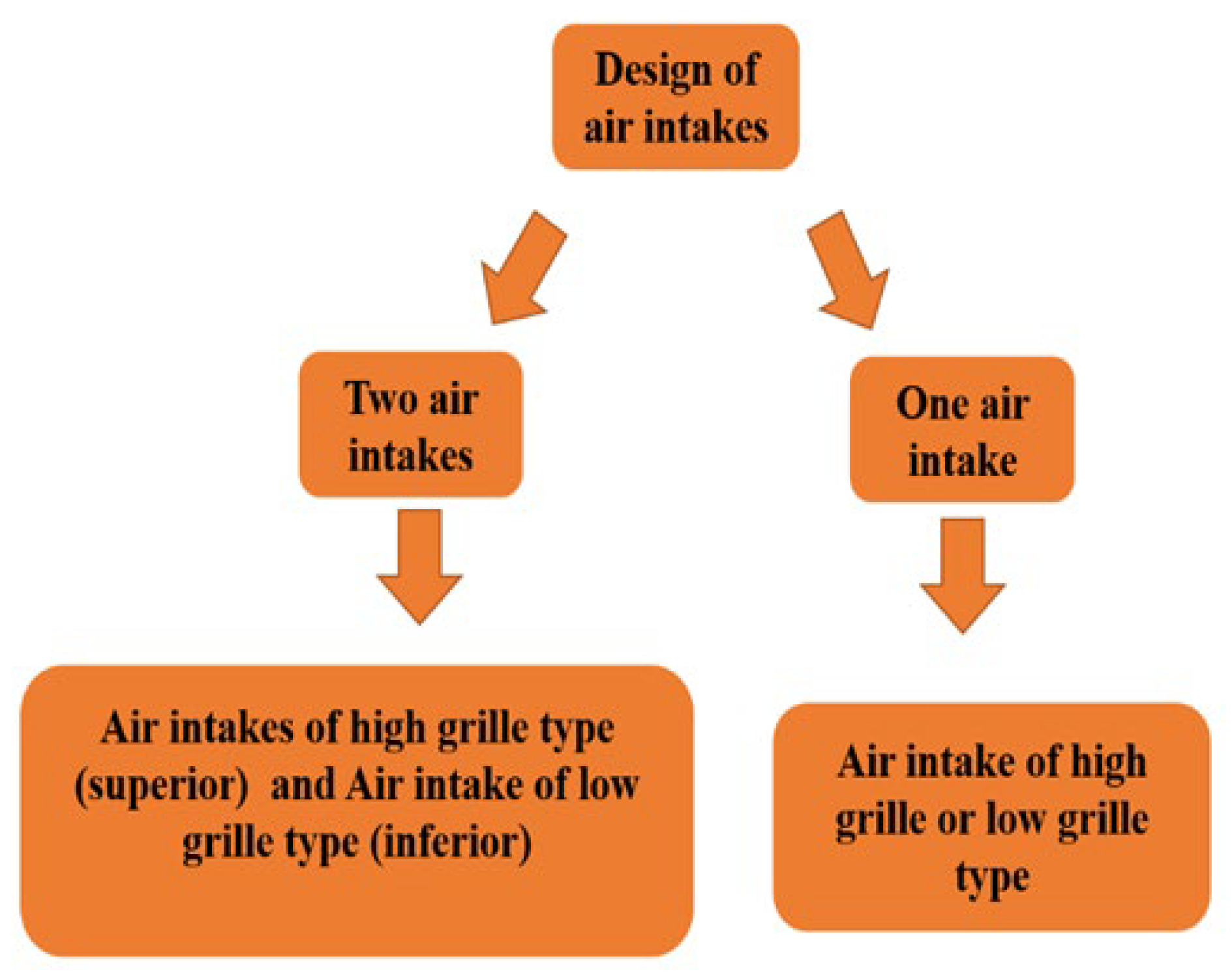
16]. Furthermore, the tube-and-fin is one of the best layouts that could be used for air-water heat exchangers. The water circulates in the tubes of elliptical cross-sections and the air flows between the fins. Generally, in the automotive industry, there exist two types of front-engine air intakes: the high lattice air intake and the low lattice air intake [
7]. Air intake designs can be classified as described in
Figure 1.
These designs are highly dependent on compromises that must take place between aerodynamic and thermal requirements so that components in the underhood function soundly. These front-end openings induce non-uniform upstream airflow velocity distribution over the first exchanger at their downstream (most commonly the condenser of the vehicle) where a part of its area will be cooled by a given velocity and the rest of the overall area will be cooled by small or negligible velocities.
Researchers have performed extensive studies and analyses on the non-uniformity of air velocity to predict how various types of air-liquid exchangers will thermally perform under these maldistributions, including ranges of industrial applications and functioning parameters. Beiler and Kroger [
17] reported that non-uniformity in the distribution of airflow leads to a decrease in the performance of heat exchangers. Nonetheless, these reductions could be neglected when using elegant air-cooled exchangers. In addition, simulation programs to calculate the influence of uniform liquid flow with non-uniform airflow have been developed by researchers. T’Joen et al. [
18] presented a computational tool that facilitates obtaining well-organized heat exchanger design configurations and showed that exchanger performance deteriorates due to airflow maldistribution.
Mueller [
19] showed that the performance of the heat exchanger depends on the type of airflow. For turbulent flow, the impact on the performance of the heat exchanger is minimal, whereas the impact is more significant for laminar flow. Mao et al. [
20] investigated the thermal aspects of the performance of a louvered fin-and-tube heat exchanger and its pressure drop when subjected to airflow maldistribution, obtaining 6% and 34% as the maximum reduction capacity and pressure drop increment, respectively. Chin and Raghayan [
21] adopted a statistical approach and found that the thermal performance of the fin-tube heat exchanger is influenced by the mean, skew, and standard deviation of a non-uniform airflow profile, but not its kurtosis.
Kaern et al. [
22] numerically investigated the performance of an evaporator under maldistributions in the feeder tube bend, inlet liquid/vapor phase, and airflow. It was demonstrated that the cooling capacity in addition to the coefficient of performance are reduced in case of misdistribution in airflow.
Fin-and-tube heat exchanger, which is the dominant HX type in automotive applications, was investigated by Khaled et al. [
23] to understand the impact of airflow velocity maldistribution on its performance. Results revealed a clear effect of non-uniformity on the HX’s performance, as a thermal performance reduction of up to 35% occured for maximum degrees of velocity maldistribution (represented by a ratio of 1 of the velocity distribution standard deviation to its mean).
Huang and Wang [
24] provided 3D U-type compact parallel flow HX designed to obtain a uniform tube flow. Chu et al. [
25] numerically simulated four novel designs through computational fluid dynamics to obtain a uniform inlet flow for a HX in high-temperature applications. A 52% non-uniformity reduction was obtained for a manifold with helical baffles which induced a 24% increase in the Nusselt number.
Yaici et al. [
26] investigated, through CFD-3D simulations, the effect of inlet airflow non-uniformity on thermo-hydraulic performance. An enhancement or deterioration of up to 50% in the Colburn
j-factor was observed in comparison to a HX with a maldistributed inlet air velocity profile.
The existence of airflow non-uniformities in compact heat exchangers was reviewed by Singh et al. [
27]. The review was performed in terms of temperature and flow and their effects on the performance of different energy transfer equipment. A decline of the thermal performance of many types of equipment due to the flow non-uniformity effect was reported.
Therefore, based on the aforementioned studies of heat exchanger thermal performance in relation to upstream airflow velocity maldistribution, the following two points can be made:
Performance deterioration due to airflow maldistribution is evident and well-proven in liquid-air heat exchangers;
Scarce are the studies that take advantage of controlling or acting on the airflow non-uniformity to improve HX performance (by reducing airflow non-uniformity).
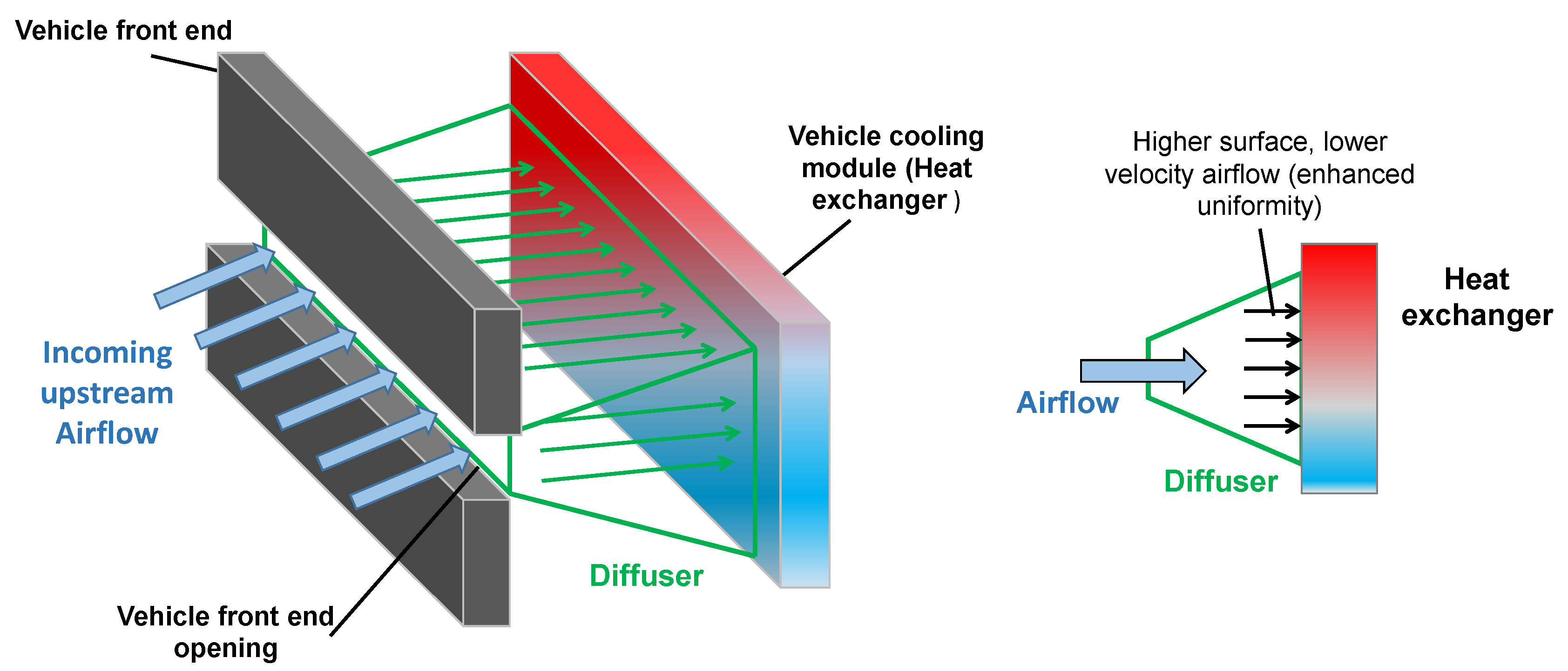
In this context and as depicted in
Figure 2, the present manuscript suggests a new concept of integrating a diffuser downstream of the vehicle’s front air intake and upstream of the first exchanger such that the non-uniformity in the airflow velocity distribution is reduced and the thermal performance of water-air heat exchangers is improved. Diffusers, in terms of physical parameters, are devices that decrease the velocity but increase the pressure. Diffusers are known for providing a more uniformly distributed flow which is evident in their use in heating, ventilating, and air conditioning systems [
28] to supply rooms with an evenly distributed conditioned airflow. Diffusers also serve the purpose of slowing the compressor airflow and increasing its uniformity before entering the combustion chamber in a jet engine [
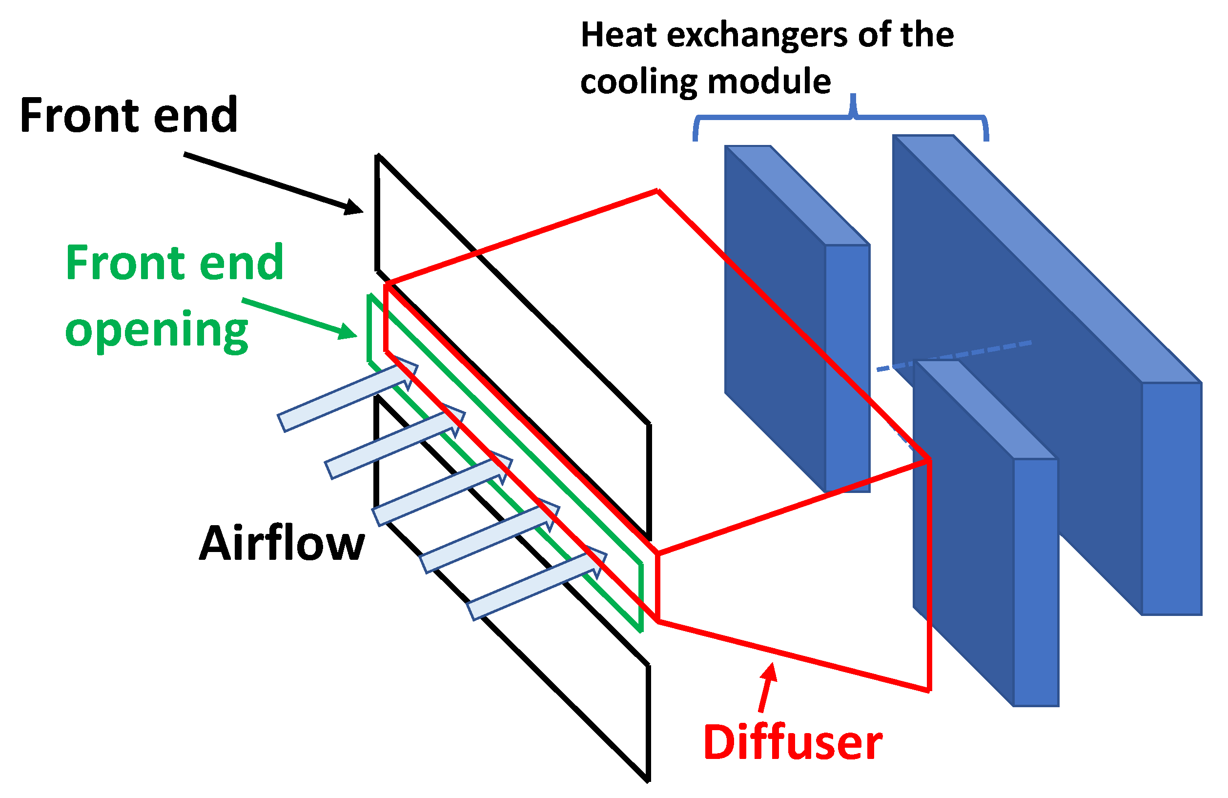
29], hence the motivation to utilize diffusers in a vehicle’s cooling module, as shown in the complete setup illustrated in
Figure 3.
It is obvious that the diffuser causes a reduction in the velocity magnitude of the flow supplied to the HX. Moreover, while the flow rate is the same at the air inlet opening and over the area of the exchanger such that the velocity distribution has the same mean velocity, the standard deviation is now lower, i.e., more uniform airflow velocity distribution. This decrease in air non-uniformity will increase thermal performance. Based on the above, parametric analyses that included the effect of various parameters was considered in
Section 4. The parameters considered are detailed below:
Area ratio of the inlet opening to that of the HX.
Diffuser length, i.e., the distance from the air inlet to the first HX.
Diffuser angle and the mass flowrates of water and air.
Calculations were done using an in-house computational code that is detailed in
Section 2.
Section 3 is then devoted to the experimental validation of the code.
Section 4 presents then the results and observations. Then,
Section 5 exposes details on energy consumption and carbon dioxide emission reductions. Finally,
Section 6 draws the main conclusions of the work.
2. In-House Computational Code
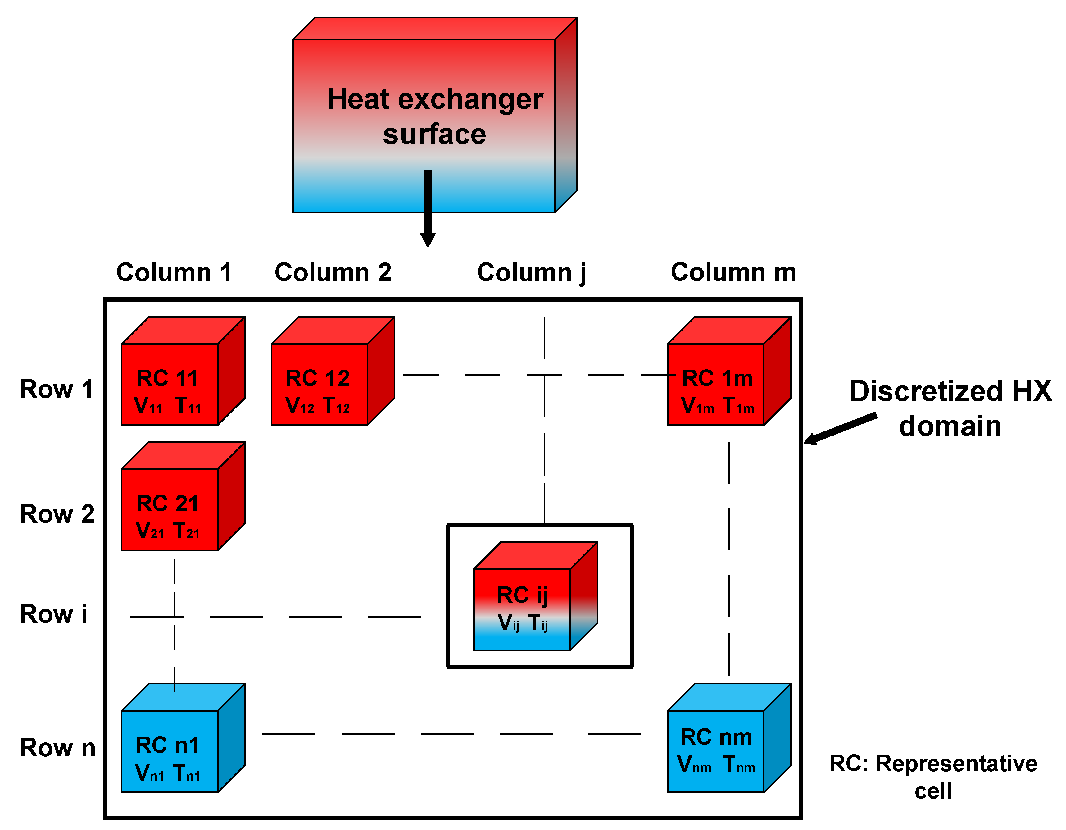
The in-house computational code is different from the standard finite element, difference, and volume techniques-based software platform. The main difference is that the standard software platforms draw the geometry of the considered element and consider the complex details of this geometry while the suggested in-house computational code considers the geometry of the heat exchanger as a black box and its effect is represented in the experimental determination of the overall heat transfer coefficient. Another important difference is that the in-house computational code relies on correlations obtained from preliminary experimental tests, mainly for the overall heat transfer coefficient. Finally, the main advantages of the in-house developed code are its low computational costs in terms of CPU time and memory space. When compared to a finite element or finite volume, the computational cost of the method is almost negligible. The method is motivated by the fact that the conditions that the heat exchanger may undergo are not necessarily uniform. In other terms, non-uniform conditions may occur in some applications such as non-uniform temperature field distribution or fluid velocity field distribution. The standard heat exchanger modeling approach that considers the heat exchanger domain as one unique patch becomes inaccurate. In other words, it becomes inevitable to adopt an approach that allows taking the non-uniform operational conditions into consideration.
The proposed method facilitates expressing the non-uniform conditions that may be experienced by the heat exchanger, this is achieved by dividing the HX into multiple elements denoted by “Representative Cells” (RC), as shown in
Figure 4.
Consequently, obtaining the outlet temperature of each RC, and finally, the overall HX outlet temperature (simultaneously HX thermal performance) is carried out by:
It should be noted that in the present study, the flow rate of water in each heat exchange tube is uniform.
The global heat exchanger problem is written in terms of overall heat-transfer coefficient
and thermal performance
according to the expression of Equation (1) [
30,
31]:
where
is the heat exchanger area, and
is the arithmetic difference of temperature given by:
where the inlet and outlet temperatures of the liquid through the HX are respectively
and
,
is the air temperature upstream of the exchanger, and
U the overall heat transfer coefficient of the HX calculated as a rational function of the heat exchanger liquid flow rate
and the cooling airflow rate
. By combining the equations of the rate of heat exchange between the two fluids at each cell and the energy balance on the exchanger liquid side between the entrance and the exit of a cell the outlet temperature can be written as follows:
where
a and
b are written in terms of the parameters of the fluids.
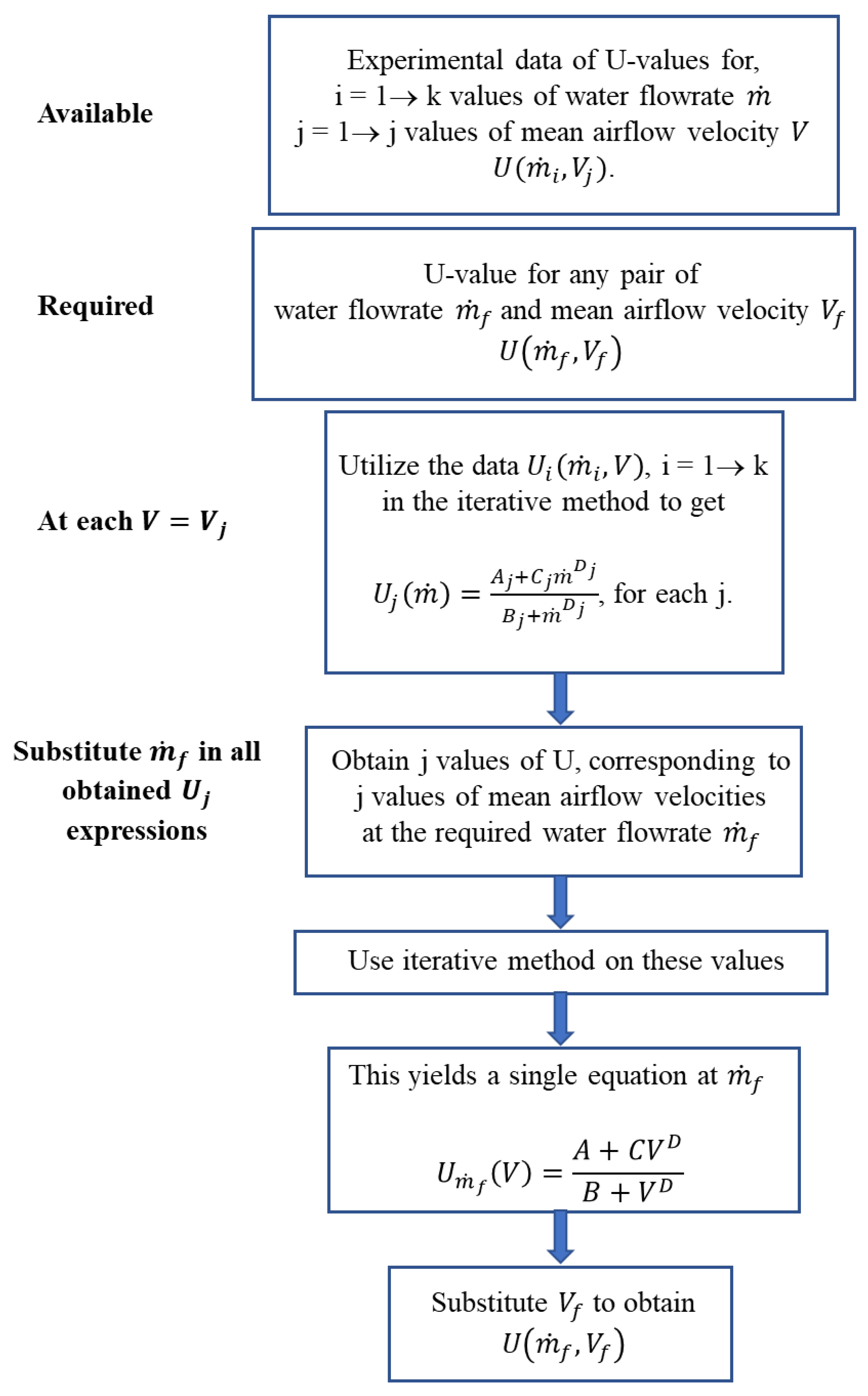
The method used to obtain the overall heat transfer coefficient of the heat exchanger is provided below.
Overall Heat Transfer Coefficient
Experimental data obtained by experiments done on the exchanger alone yield distinct
U values of the exchanger such that for every couple of fluid flow rates
and airflow mean velocity
, a value of
will be obtained, which is assigned at the representative cell level traversed by the aforementioned couple of liquid flowrate and airflow mean velocity. The extrapolation technique of the code permits then to develop a general expression that determines the overall
value of a representative cell of the exchanger traversed by any couple of liquid flowrate and mean airflow velocity. To proceed, the method is based on rational extrapolation functions [
30] of the general form:
with
,
,
, and
being constants to be determined. The idea of the extrapolation method is to obtain these constants by a set of experimental points
where
(
is the number of experimental points). The iterative procedure starts by assuming a
D value, yielding the algebraic system:
The solution of the system of Equation (5) by utilizing three points
of the experimental data provides the three constants
,
,
as follows:
Then, the value of
will be adjusted iteratively so that the error vector’s magnitude is minimized:
where
is the error vector,
is the vector of experimental data obtained for the overall heat transfer coefficient, and
is the vector of overall heat transfer values obtained using the rational function of Equation (5). The iterative method presented above is then followed to obtain the overall heat transfer coefficient
of an exchanger operating with a prescribed couple of liquid mass flowrate and mean airflow velocity
.
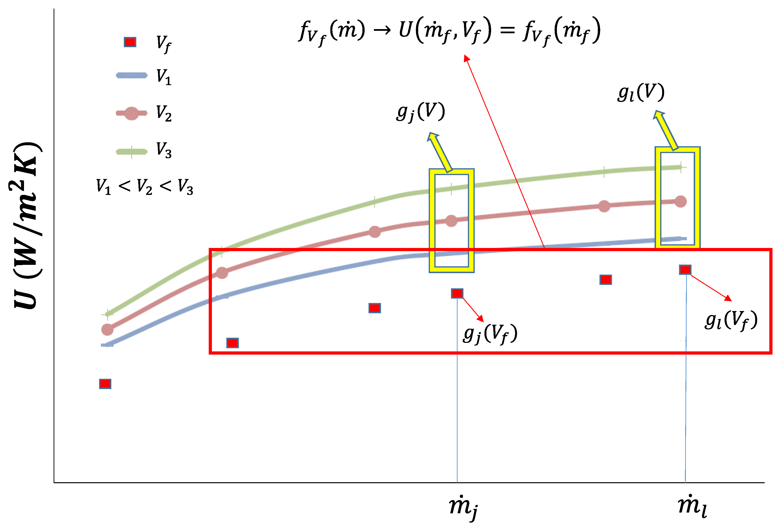
Figure 5 shows an illustration of the method used to obtain the overall heat transfer coefficient for a given couple
.
For each mean air velocity
(for
,
is the number of experimental data corresponding to
different configurations of mean air velocity), the functions
are obtained from
experimental values
(nodal values) using the iterative method presented above:
Thus, with the obtained
expressions
,
nodal values
are obtained from liquid mass flowrates
. From these values,
is also determined using the iteration method presented above:
Lastly, the exchanger’s overall heat transfer coefficient can be obtained using the following expression:
An illustration of the U-value estimation with the developed code is shown in
Figure 6.
3. Experimental Validation
In this section, numerical data are associated with their experimental equivalents. Comparisons are done for the overall heat transfer coefficient (
Section 3.2) and the thermal performance of the exchanger (
Section 3.3). The experimental setup used to obtain experimental data is presented in
Section 3.1.
3.1. Experimental Setup
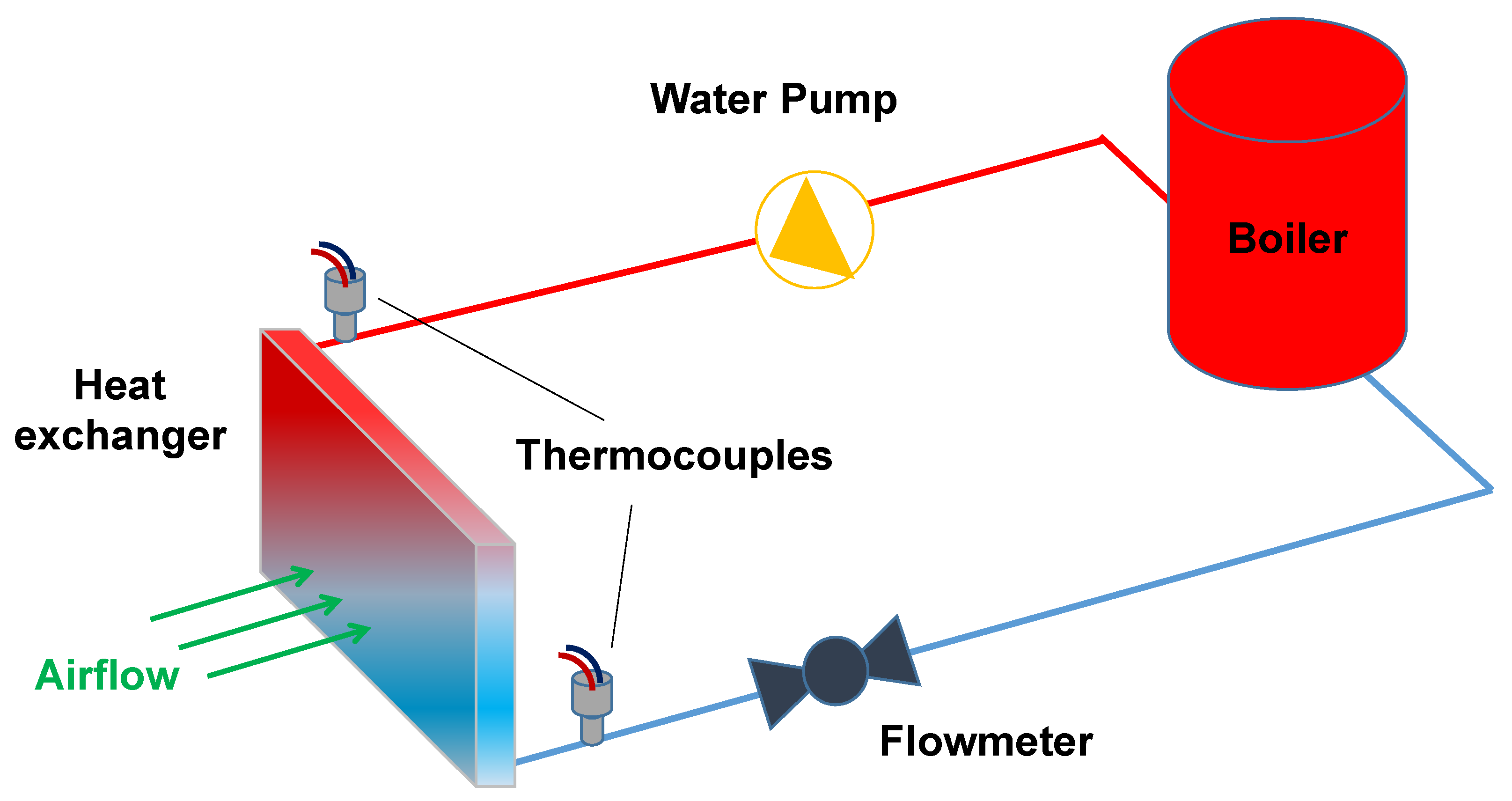
The objective of the experimental setup is to measure the heat exchanger’s performance for several configurations of airflow velocities and water flow rates. The schematic of the experimental setup is shown in
Figure 7.
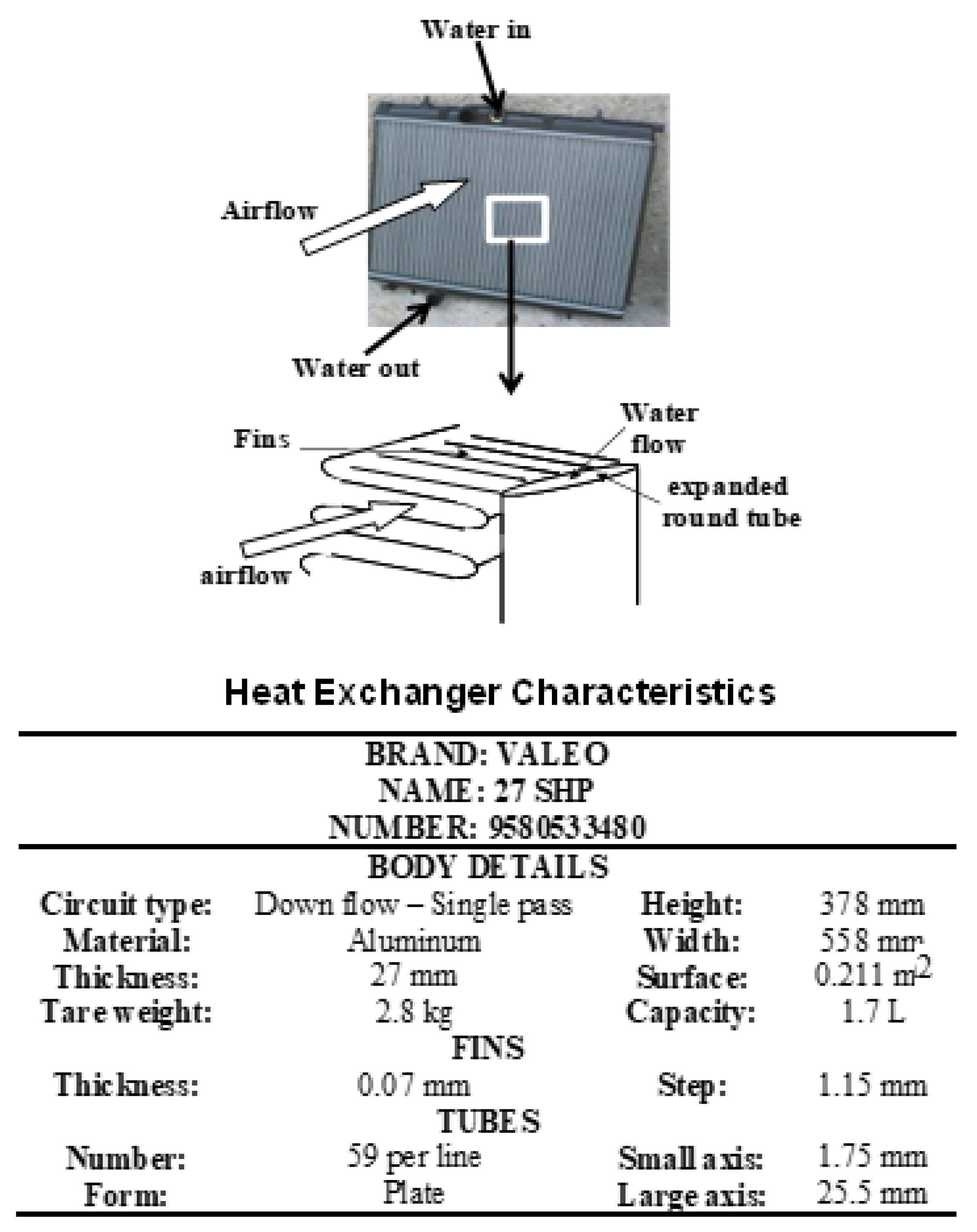
The heat exchanger used in the experimental setup is a tubes-and-fins type that has the structure and characteristics shown in
Figure 8.
Inlet hot water of any desired inlet temperature can be provided to the HX using the circuit shown.
The thermal circuit of the experimental setup essentially comprises a boiler of variable power, a radiator (fin-and-tube, air to water, airflow of different velocities provided by wind tunnel) of a real vehicle (Peugeot 207), the main water supply, a flowmeter, small taps, and traps.
The boiler has a built-in pump with several speeds and a temperature sensor that allows setting the hot temperature (the temperature at the radiator inlet) according to prescribed values. Three thermocouples are used to provide measurements of the water’s inlet and outlet temperatures as well as the upstream air temperature. Thermocouples used are type T thermocouples having ±1 °C or ±0.75% of accuracy.
Temperature recordings are taken for specified airflow velocity and water flow rate values. The obtained experimental data permit the estimation of the overall value using Equations (1) and (2). The air velocities tested are 0.5, 1, 2, 3, 4, 5, 6, 7, and 8 m/s and the water flowrates tested are 1500, 3000, 5000, 6000, 8000, and 9000 L/h; which corresponds to 60 configurations of a couple of water and airflow rates where the corresponding overall heat transfer coefficient is measured. Air velocities are measured using a pitot tube having an accuracy ranging from 0.5% to 5%. The flowmeter used has an accuracy of 0.10%.
3.2. Comparisons of Overall Heat Transfer Coefficient
In this part, the experimental validation of the method of estimation of the overall heat transfer coefficient (extrapolation method) of
Section 2 is presented.
To proceed, the rational function of the overall heat transfer coefficient is calculated based on the airflow velocity values varying from 0.5 to 7 m/s for each curve. Then, the overall heat transfer coefficient is determined for an airflow velocity of 8 m/s for multiple water flow rates by means of the rational function extrapolation method. The calculated overall values are then compared to the data obtained by the experimental setup.
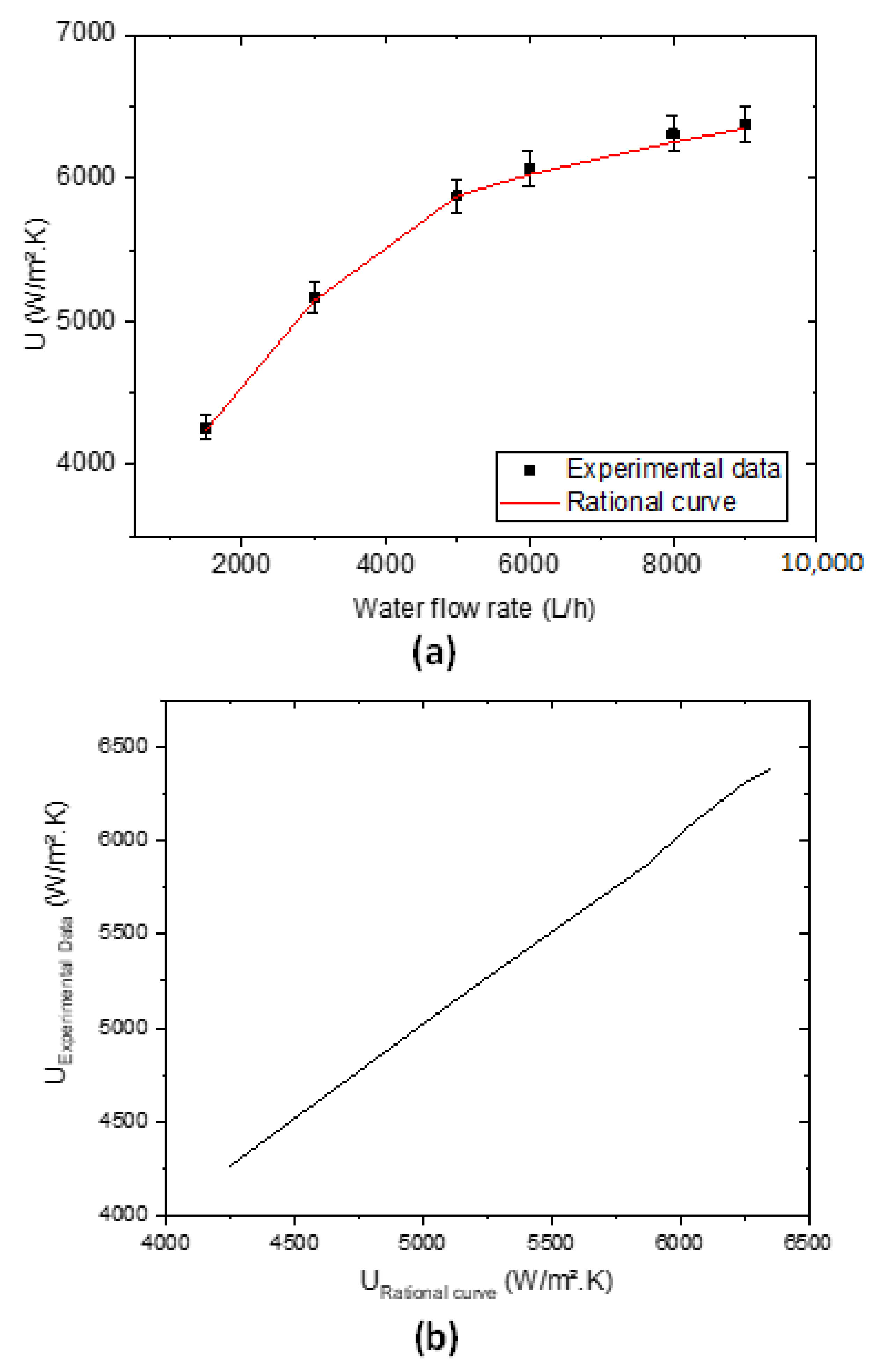
Figure 9 shows the overall
U value using the extrapolation rational method versus those obtained experimentally (
Figure 9a) as well as the relative error of determining the overall heat transfer coefficient with the rational function method (
Figure 9b).
As shown in
Figure 9a, the overall heat transfer coefficient variation obtained with the rational function method fits very well with the experimental behavior. To exemplify, at a water flow rate of 6000 L/h, the overall heat transfer coefficient conveys an experimental value of 6066 W/m
2 K while an estimation of 6024 W/m
2 K is found with the rational function.
In terms of relative error, it ranges from 0 to 0.9% as the water flow rate changes between 1500 and 9000 L/h. Therefore, the rational function method calculates the overall heat transfer coefficient with an average relative error of 0.47%. Similarly, the same procedure is followed for all air velocities and water flow rates, yielding results of the same order of magnitude. Therefore, the semi-analytical rational function method is valid for obtaining the overall heat transfer coefficients.
3.3. Comparisons of Thermal Performance
This section concerns the experimental validation of the whole scheme of the in-house computational code. For this purpose, one of the most important outputs of the code which is the exchanger’s thermal performance is selected. To proceed, an exchanger with a water flow rate of 6000 L/h is considered. Water is considered to enter the exchanger at 95 °C while the air upstream of the heat exchanger is considered to be at a temperature of 20 °C. Simulations with the code were performed for an air velocity ranging from 1 to 8 m/s.
Figure 10 presents the evolution of the exchanger’s performance as a function of airflow velocity using the in-house computational code and experimentally obtained data (
Figure 10a) as well as the relative error of determining the thermal performance with the in-house computational code (
Figure 10b).
From
Figure 10a, it is clear that the variation of the performance obtained with the computational code fits very well with the experimental behavior. To illustrate, at an airflow velocity of 6 m/s, with respect to the thermal performance of 74.9 kW obtained experimentally, the thermal performance determined with the computational code is 73.1 kW.
As for the relative error, it varies between 0.43% and 3.76% when the airflow velocity varies between 0.5 and 8 m/s. Therefore, the computational code calculates thermal performances with an average relative error of 1.86%. The above procedure was used for multiple ranges of air velocities and water flow rates, giving the same orders of magnitude.
Therefore, the computational code has sufficient accuracy and precision to calculate thermal performance and overall heat transfer coefficient. The next section will be devoted to the use of the in-house computational code to obtain results for the new design suggested (use of diffusers in cooling modules of vehicles).
4. Results, Observations, and Discussions
In this section, parametric analysis on the enhancement of the heat exchanger’s thermal performance, with the novel setup of introducing a diffuser ahead of the cooling module is presented by employing the above-mentioned code.
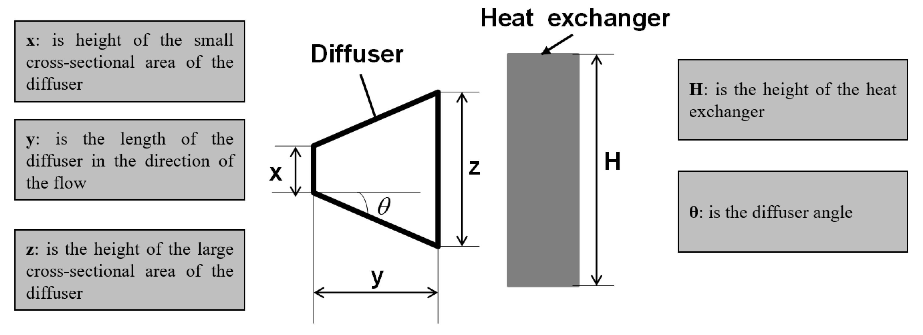
Figure 11 portrays an illustration of the proposed exchanger-diffuser setup along with the main parameters is presented.
The relation between the diffuser’s geometrical parameters is expressed by:
Normalization of the parameters
x,
y, and
z is done with respect to the heat exchanger’s length as shown in the following equations:
A maximum value of the diffuser’s large cross-sectional height is set to prevent it from exceeding the heat exchanger’s height. Moreover, a suitable spacing between the exchanger and the vehicle’s front opening must be chosen.
The first calculation set is performed for a 6000 L/h water flow rate and 7 m/s airflow velocity. The inlet temperature of water is set at 90 °C and that of air at 20 °C. The angle of the diffuser is fixed at 30°. Under these conditions, for multiple values of ratio
X (0.2, 0.3, 0.4, and 0.5), ratio
Y is varied from zero to the highest permitted value.
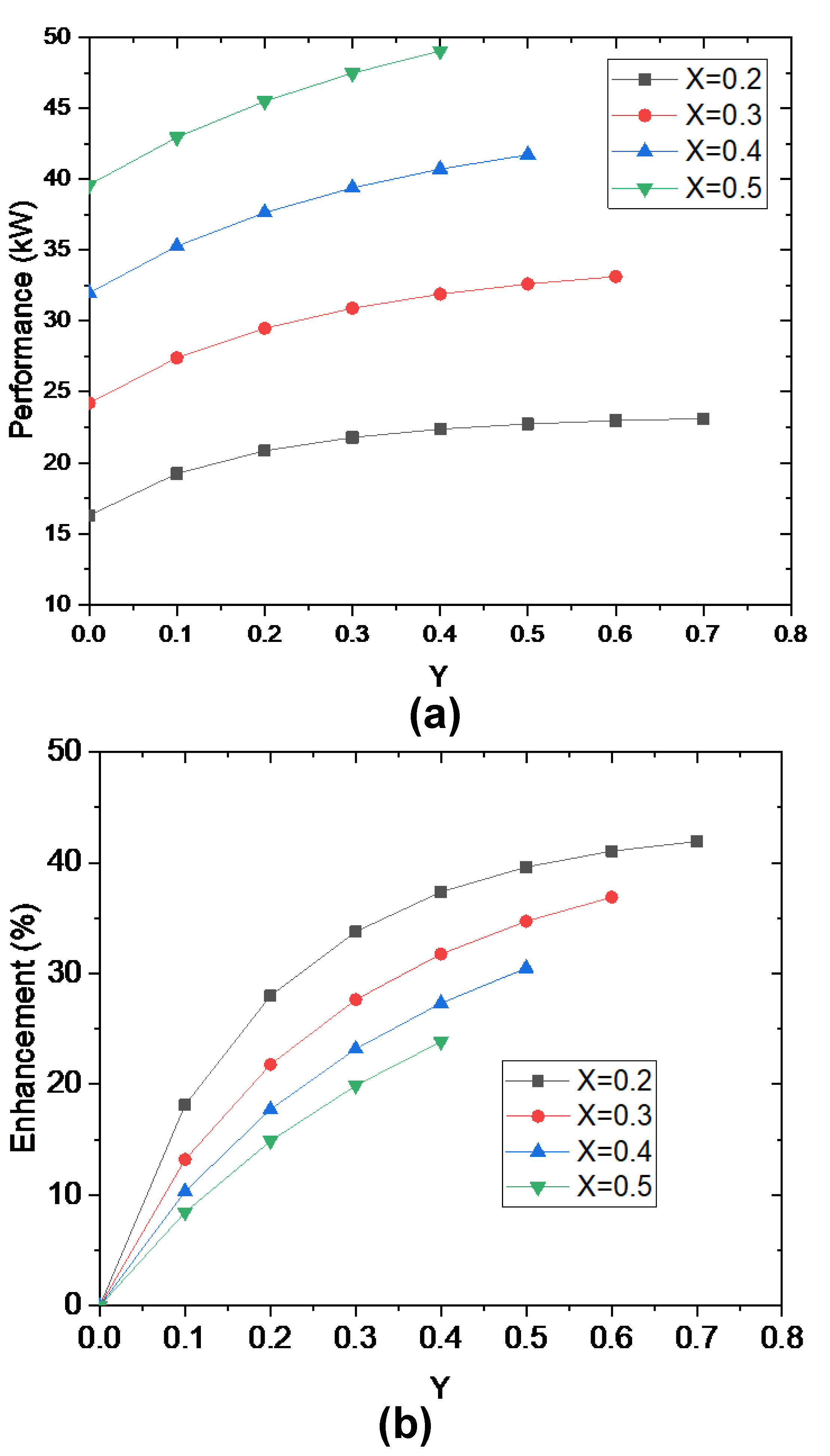
Figure 12a shows the variation of the heat exchanger’s thermal performance with a diffuser, and
Figure 12b represents the percentage of its enhancement evaluated in reference to the case without a diffuser (
Y = 0).
The performance enhancement percentage indicates the additional heat removal from the water stream with the inclusion of the diffuser relative to the basic case where no diffuser is added.
As shown in
Figure 12, as the ratios
X and
Y increase, the thermal performance increases. However, the enhancement of the performance decreases with the increase of
X. To elaborate, for a ratio of
X = 0.2 (i.e., an air inlet opening height of about 20% of that of the HX), when
Y increases from 0 to 0.7, an increase from 16.3 to 23.1 kW is observed in the thermal performance. To further illustrate, when
Y is increased from zero to its maximum value which becomes 0.4 at
X = 0.5, an increase from 39.6 to 49 kW is observed in the thermal performance. As for the performance enhancement (which increases with
Y and decreases with
X), it reaches a maximum of 41.9% for the
X = 0.2; while for
X = 0.5 a maximum enhancement of 23.8% is achieved. Therefore, to have the best improvement it is therefore necessary to provide a fairly long diffuser (large Y) and with a small height of the small cross-sectional area (X).
The second set of calculations is undergone with a 20 °C upstream air temperature and 90 °C water inlet temperature (same conditions as the first set). The ratio
X is taken to be equal to 0.3. The ratio
Y is fixed at 0.3 and the angle of the diffuser is fixed at 30°.
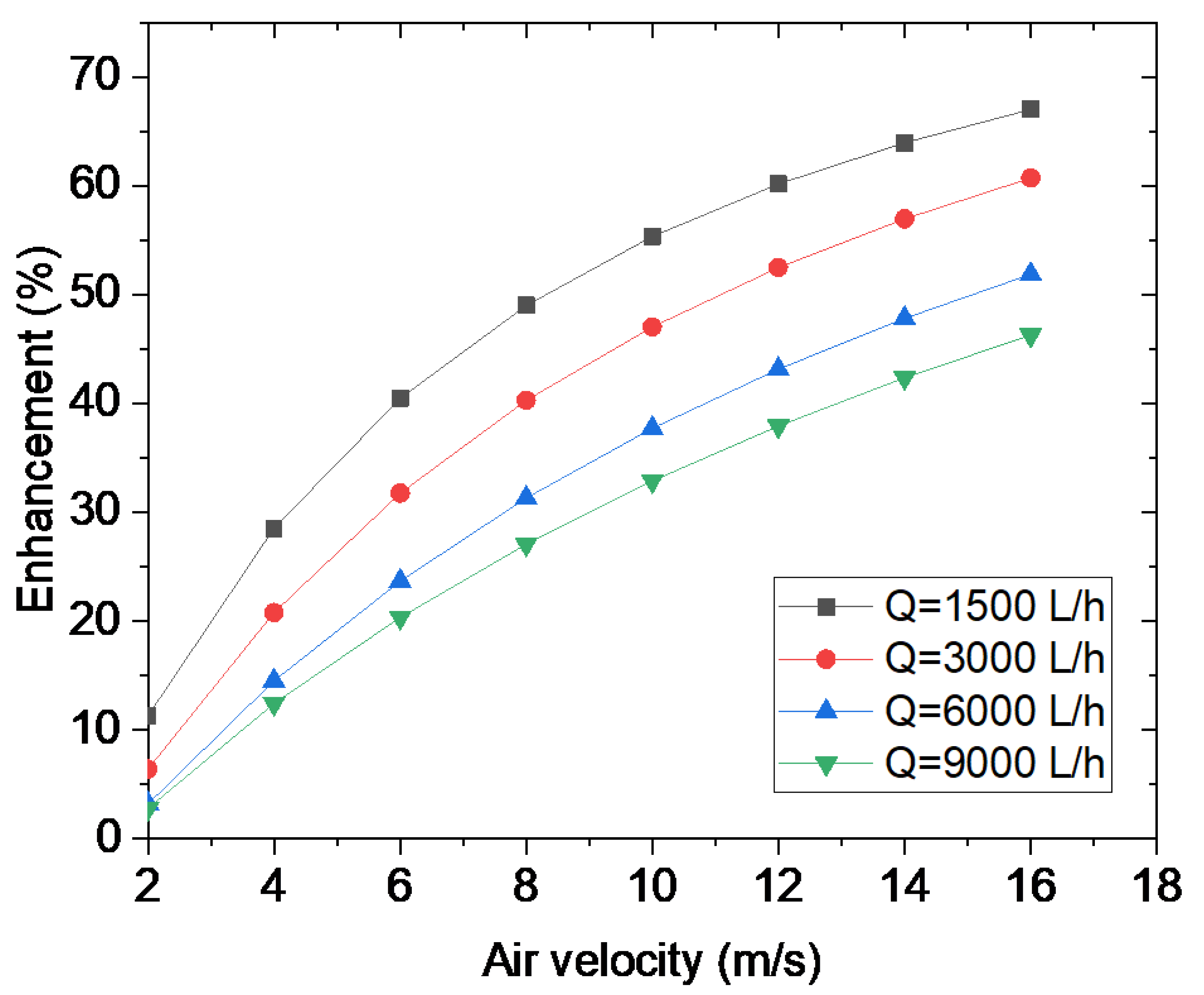
Figure 13 provides the outcomes of the heat exchanger performance enhancement that is obtained in reference to the case without a diffuser (for Y = 0) with respect to air velocity at the air inlet opening for different water flow rates.
It is observed in
Figure 13 that the percentage of thermal performance enhancement increases as air velocity increases. As illustrated, at 1500 L/h water flow rate, as the velocity is increased from 2 to 16 m/s, enhancement of the performance leaps from 11.3 to 67%. Moreover, with a 9000 L/h water flow rate and the same range of airflow velocity, the performance enhancement rises from 2.8 to 46.3%. Finally, the enhancement provided by the introduction of the diffuser is larger at high air velocities and low water flow rates.
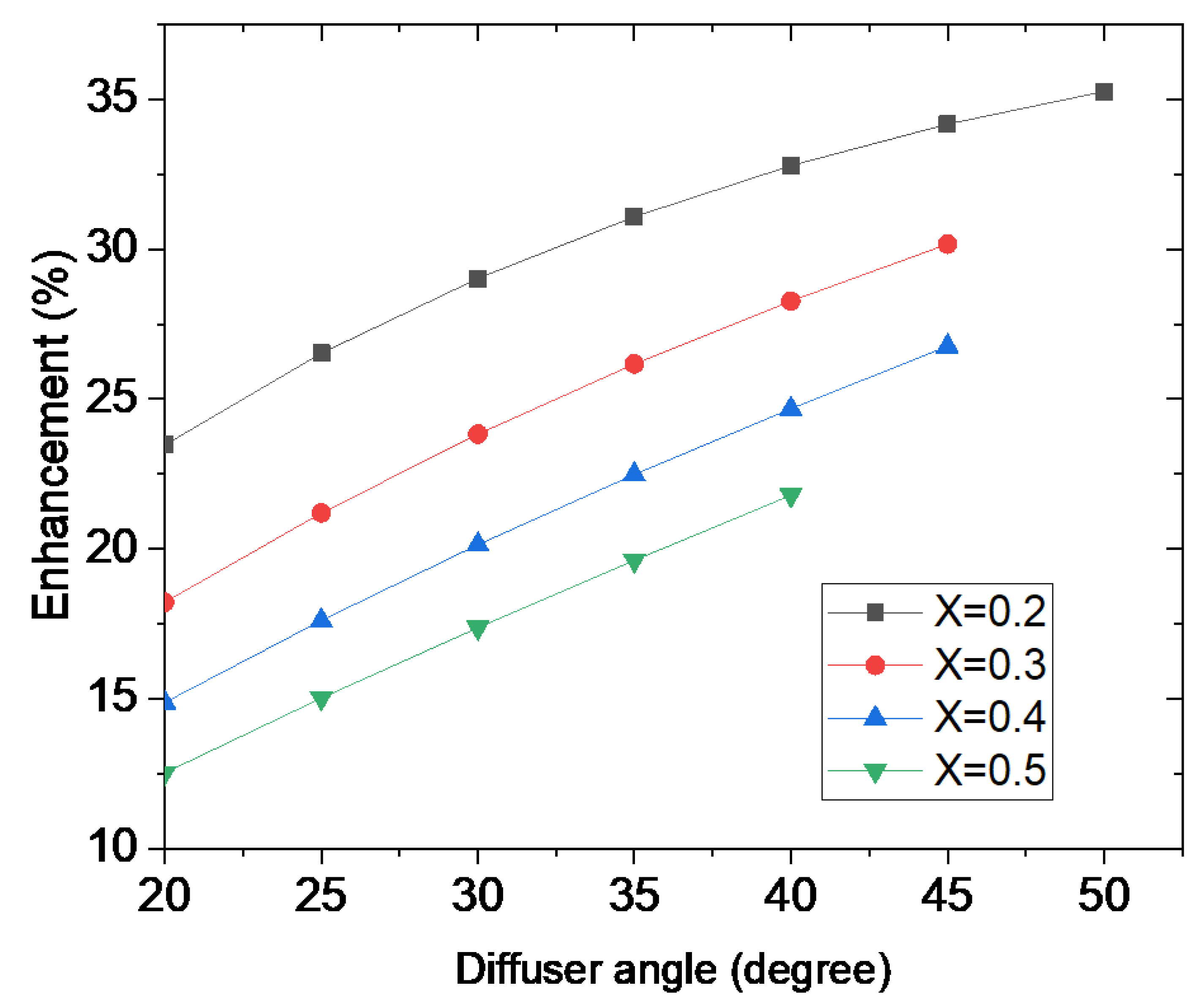
The third set of calculations is performed with an inlet water flow temperature of 90 °C and upstream air at 20 °C (same conditions as the first and second sets). Air velocity is set to 7 m/s, water flowrate of 9000 L/h is chosen and
Y is fixed at 0.3. The diffuser angle is varied for multiple values of ratio
X. Consequently,
Figure 14 shows the percentage of performance enhancement evaluated in reference to the case without a diffuser (Y = 0).
As mentioned previously, the inlet diffuse area is set to a certain value (
X = 0.2, 0.3, 0.4, or 0.5), while the distance between the HX and the inlet opening is constant throughout (
Y = 0.3). The trend of the curves clarifies that the thermal performance enhancement increases when the diffuse angle increases. To illustrate, with
X = 0.2, a 13% increase in performance enhancement is achieved when increasing the angle of the diffuser from 20 to 55°. It is interesting to note that this improvement is lesser at larger
X. For
X = 0.5, increasing the angle of the diffuser from 20 to 40° causes an increase in the performance enhancement of 12.5 to 21.8%. It must be observed in
Figure 14 that an upper limit exists for the diffuser angle depending on the value of
X else the diffuser’s outlet section would be greater than the exchanger’s area.
5. Energy and Environmental Calculations
Now, to quantify the percentages of energy consumption reduction that can be achieved with the suggested novel design, a condenser-radiator cooling module is considered downstream. For each exchanger, namely, the radiator and the condenser, the novel design is considered to result in an enhancement ratio
defined as:
where
is the exchanger’s performance with the new design implemented and
its thermal performance in the original design (i.e., without the new design implementation) and
is the enhancement presented in
Figure 12,
Figure 13 and
Figure 14.
Now, the enhancement of the exchanger’s thermal performance can be seen as a reduction of the flow rates of the radiator’s water and the condenser’s refrigerant by a factor
to have the same performance as the exchanger. These flow rate drops induce reductions of approximately
of the pump’s power requirement
; and
of the HVAC compressor’s power requirement
, where
COP is the HVAC system’s coefficient of performance. Then, the power consumption reduction
PCR is:
Then, Equations (19) and (20) express the input power consumption reduction
IPCR and the fuel consumption reduction
FCR, respectively:
where
is the efficiency of the engine and
the heat of combustion of the fuel. For vehicles with powertrains ranging from 100 kW to 200 kW, the maximum powers
and
needed to operate the water pump and the compressor are respectively about 10 kW and 4 kW [
7,
32]. Moreover, the
COP for most of the HVAC systems of vehicles is around 3 [
7]. A gasoline vehicle emits, per 1 kg of gasoline, 3.28 kg of carbon dioxide, it has an average efficiency of 0.35 and 47 MJ/kg heat of combustion [
32].
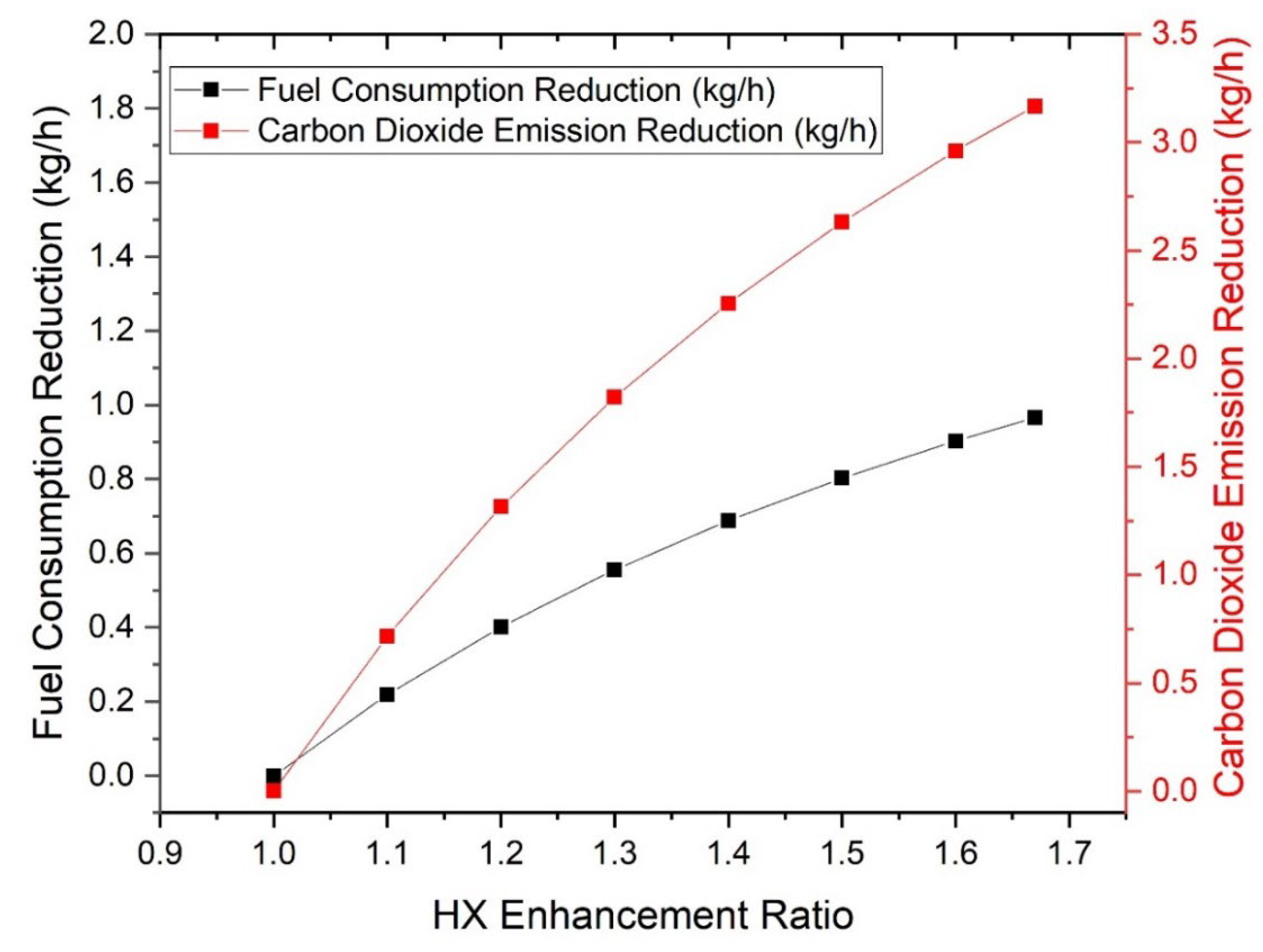
Figure 15 shows the variation of the fuel consumption reduction
FCR and carbon dioxide emission reduction
CDER (3.28 kg for each kg of gasoline burned) in function of the enhancement ratio
of the exchanger achieved with the implementation of the new design.
According to
Figure 15, it can be shown that around 0.22 kg/h of fuel consumption rate and 0.72 kg/h of carbon dioxide emission rate can be reduced if the diffuser is applied to a given configuration and increases the thermal performance of the exchanger by 10% (enhancement ratio of 1.1). These reductions can reach respectively 0.97 kg/h and 3.17 kg/h if the thermal enhancement is up to 67% (which corresponds to the maximum value obtained with the parametric analysis above). Lastly, for a vehicle that operates about three hours a day, up to 2.91 kg (3.89 L) of gasoline consumption and 9.51 kg of emitted carbon dioxide can be reduced per day.


 ,
, 


