1. Introduction
The mathematical modeling of transient processes in complicated dynamic systems is today a very important issue to both science and the national economy. An effective and highly adequate mathematical model allows for describing real physical processes in an object, as discussed in [
1,
2,
3,
4,
5,
6]. This is particularly important at the stages of design, production, and operation of complex electric power systems.
In the general case, an engineering object obviously consists of connections among subsystems of different types, very often the subject matter of various scientific domains such as power electric or mechanical engineering, hydraulics, thermodynamics, etc. Integrating these disciplines into a mathematical model may be a very complex problem. In addition, a team should have a very extensive knowledge of these disciplines to be able to develop an effective model of such a complicated object. Such an interdisciplinary research team is costly, time-consuming, and not always effective. The question is, therefore, can another method be found to combine a variety of scientific fields and thus simplify and limit the number of research team members to a necessary minimum? An affirmative answer is given in [
7,
8,
9].
The mathematical modeling of dynamic systems normally uses classic approaches, whose ideology is based on the law of energy conservation, with complex dynamic systems split into its subsystems. Each subsystem is then described with appropriate applied physics equations. The equations for these subsystems are finally combined into a sole system of dynamic state equations of an integrated object under analysis. This method suffers from two drawbacks. All implicit, latent motions cannot always be found and described, and it is hard to assemble an interdisciplinary research team that would combine all the complex phenomena to describe the dynamic system. These shortcomings are absent from variation methods, which presume interdisciplinary approaches [
7,
10,
11,
12,
13]. In these methods, the ideology of mathematical modeling of a complex object consists solely of an energetic approach. Such a system does not employ the decomposition of a sole dynamic system as the classic approaches do. A variation method determines the Lagrangian, part of the action functional as per the Hamilton principle [
8,
14,
15,
16,
17,
18]. The functional is then subjected to the minimization procedure, which enables the generation of an equation for the extremals of this functional. In effect, the Euler–Lagrange equation becomes part of the mathematical model of the dynamic system analyzed.
The ideology of variation approaches to modeling has been known for a long time [
8,
9,
12,
19]. In the general case of an ordinary interpretation, variation approaches are restricted by the conservative nature of dynamic systems. In the event, the Lagrangian is the difference between the kinetic and potential energies, which makes variation principles uncompetitive against classic principles in real conditions. To avoid this problem, the work [
7] expands the application of variation principles by extending the Lagrangian. The authors formally add the energy of dissipative forces to the kinetic energy and the energy of external non-conservative forces for the potential energy. They argue accordingly that the Hamilton principle can be applied to the extended Lagrangian.
The work [
7] is a classic in the theory of electromechanical energy conversion. It gave rise to [
8], which proposes a slightly different approach. The said additional components of the classic Lagrangian (the energy of dissipative forces and the work of external forces) are not introduced formally, but only determined mathematically, which once again validates the theory presented in [
8]. The book [
7] analyzes only lumped parameter systems. The systems of both lumped and distributed parameters are analyzed in [
8], on the other hand. Since the idea of expanding the application of the classic Hamilton principle to distributed parameter systems was developed by Mikhail Ostrogradsky, the method introduced in [
8] is defined as the Hamilton–Ostrogradsky principle. According to this principle, the development of the model of a complex object only consists of an energetic approach, and therefore an interdisciplinary method of mathematical modeling of dynamic objects is feasible at virtually any level of complexity.
A modified Hamilton–Ostrogradsky principle serves the development of a mathematical model of complicated dynamic objects of lumped and distributed parameters in this paper. We analyze a three-phase distributed parameter power supply line loaded with an RLC circuit. Three-phase power lines are commonly known as highly complicated electric power objects that feature implicit, latent motions, which we represent not only as electromagnetic phenomena. Switches are present on the line’s ends, where not only electric but also mechanical, thermodynamic, electrostatic, and other processes take place [
3,
20,
21]. The interdisciplinary approaches discussed above can be fully applied to such an electric power system.
This paper is limited to electric processes and employs field and circuit approaches. The impact of mechanical processes on similar systems is discussed in [
20]. The aim of this study is to use an interdisciplinary method of mathematical modeling, based on a modification to the Hamilton–Ostrogradsky principle, to construct a mathematical model of a three-phase power supply line loaded with an RLC circuit, and to analyze transient processes in the electric power system.
This study is not designed to compare the concepts of modeling from the viewpoint of variation and classic approaches. These concepts are well-known and, given the correct method, produce identical state equations [
20,
21]. We aimed to demonstrate that variation approaches are fully useful to the modeling of complex electric power facilities of distributed electromagnetic parameters, which has been substantiated in mathematical terms.
2. Mathematical Model
The electric power system is analyzed as a real distributed parameters system. Therefore, energetic functions, and their corresponding linear densities, are used in the modified Lagrangian [
8]. Thus, the extended Hamilton–Ostrogradsky action functional
S will be as follows [
8]:
where
S—Hamilton–Ostrogradsky action functional,
I—energetic functional,
L*,
Ll—modified Lagrangian and its linear density.
The extended Lagrangian becomes [
8]:
where
T*—kinetic energy,
P*—potential energy,
—the energy of generalized dissipative forces,
D*—energy of external non-conservative forces. The parameters subscripted as
l define the respective linear densities of energetic functions.
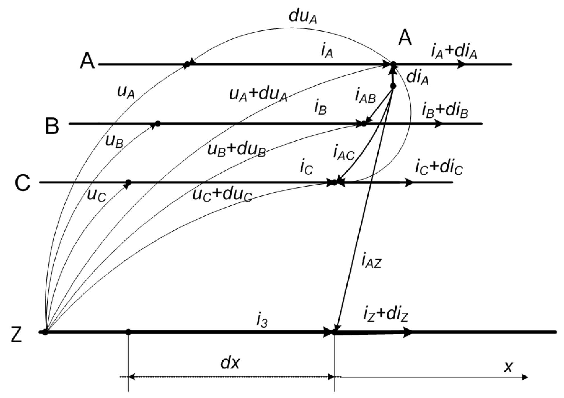
The calculation diagram shown in
Figure 1 is additionally used to prepare the model of electric power system.
The current coordinate
x along the transmission line and the length Δ
x of the line’s element are marked in
Figure 1.
The equation for scleronomic constraints in the steady state (Kirchhoff’s first law) for the transmission line element is expressed as:
where
—the current across phase A wire along the Δ
x; Δ
iAZ—the component of summary leakage current between the phase A wire and the zero (earth) wire; Δ
iAB—the component of summary leakage current between the phase A and B wires; Δ
iAC—the component of summary leakage current between the phase A and C wires.
Integrating (3) with respect to time also for phases B and C, where
under zero initial conditions, produces:
where
—the respective charges along the line length Δ
x for phase A (and phases B and C, respectively), cf. (3).
The charges in transmission line elements are expressed as [
22]
where
uij(
x,
t),
i ≠
j—line-to-line voltages;
Cij,
i ≠
j—the respective line-to-line distributed capacitances,
i,
j =
A,
B,
C,
C0—the line-to-ground distributed capacitance.
Equations (3)–(5) can be expressed for
as a matrix equation in the form of rectangular arrays:
where
On the basis of Faraday’s law of electromagnetic induction and Kirchhoff’s voltage law, the equations for the three-phase circuit shown in
Figure 1 were formulated. The equation for phase A is given as (8), wherein
, Δ
x → 0 so Δ
x → ∂
x, while the equations for phases B and C are analogous.
where Δ
uj,
j =
A,
B,
C—changes in phase voltages along Δ
x;
L0,
R0—the distributed inductance and resistance (per unit length) of the transmission line;
Mi,j;
i ≠
j—distributed mutual inductances between the respective line wires;
RZ—distributed earth resistance;
iZ = −
iA −
iB −
iC—current flowing in the earthing conductor.
Dividing the left and right sides of (8) by Δ
x, where Δ
x → 0, and taking into account analogous equations and transformations for phases B and C, and then using the matrix notation in the form of rectangular arrays, we obtain the following equation:
Equations (6) and (9) will now be written in the symbolic matrix notation:
where
Q =
Q(
x,
t)—the column vector of phase charges in the transmission line;
i =
i(
x,
t)—the column vector of phase currents;
u =
u(
x,
t)—the column vector of phase voltages;
C0,
R0,
L0—the matrices of transmission line parameters.
When the three-phase line is symmetrical, the following dependencies can be written [
23,
24,
25]:
The matrix parameters in (10) and (11) will be simplified as a result:
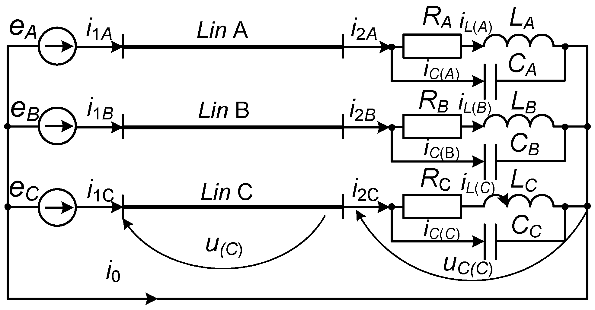
In the context of this paper, the symmetrical three-phase power line is loaded with an unbalanced RLC circuit. This operating variant will be treated as simplified.
Figure 2 illustrates a circuit diagram of the electric power system tested here.
The generalized coordinates for the energetic functions of the extended Lagrangian [
8] will be introduced to the system’s model:
—charges in the load’s branches and the space functions of the generalized coordinates:
—charges in the line phases of the distributed parameter system and generalized velocity functions are —currents across the load branches and —currents across the line wires, respectively.
The linear energy densities in the non-conservative Lagrangian are obtained using the known formulas for kinetic and potential energies in a transmission line, as well as the formulas for the linear densities of the external and internal electric energy dissipation [
8,
22].
The following equations will be written on the basis of (2):
where
—line-to-ground and line-to-line conductivity, respectively.
Not the sum total, but the difference in the two terms of the function elements is a crucial moment in determining Φ
l. This is related to the fact that the first term of (17) represents energy losses across the line wires and losses due to the current flow across the ground, whereas the second term represents another loss type, associated with leakage currents of the power line. When energized, the power line absorbs from the space the electromagnetic energy being generated by a source of electromagnetic energy, while the line wires merely indicate the direction of energy flow. Therefore, the minus appears in (17) [
22].
The following equation will be written on the basis of (10) and (13):
where
We assume again that the current does not flow across the line at the initial time and leakage currents are absent from the transmission line. In the circumstances, the external and internal electromagnetic energy dissipations are zero at the initial instant in time, that is, .
On considering (16), (20), and (21), the equations for potential energy become:
where
The dissipation energy will be calculated as follows:
where
In order to arrive at an equation of action functional’s extremals as per Hamilton–Ostrogradsky, the functional variation (1) must equal zero. This is equivalent to a simultaneous zeroing of the equation components (1):
The variation is derived and zeroed:
The Ostrogradsky–Gauss theorem, theorems on changing the sequence of differentiation and integration, and the law of integration by parts [
19] are used to compute the variation of two internal functionals. The assumptions presented in [
7] are used as well:
Finally, the following equations are obtained (additionally, see
Figure 2):
The equation of non-conservative external energies D* does not serve the minimization of the functional, since the electromotive force EMF is independent from the RLC load circuit, cf. (14). To address the input EMFs, boundary conditions need to be introduced to the transmission line’s equation. See (42).
Equation (30) finally produces:
or is expressed in the matrix–vector notation:
Equation (10) is differentiated with respect to the spatial coordinate and, considering (11), the equation for the scleronomic differential constraint for (34) is written:
Considering the time dependences among the functions of generalized coordinates and velocities will result in:
The equation of internal functional’s extremals, that is, the Euler (Euler–Poisson) equation, is defined by:
Transforming (37) produces:
where
The equations for the three-phase long transmission line, (38)–(40), are written in reference to the line charge. The transmission line Equation (38) is transformed into a current function by differentiating the left and right sides with respect to time. Equation (38) can also be transformed into a voltage function by differentiating the left and right sides with respect to the spatial coordinate and multiplying the left and right sides by the matrix
. This means the transmission line equation can be expressed in a unified matrix–vector notation:
An equation of three-phase power line is based on the action principle [
8]. It should be emphasized that the conductivity matrix
G0 for leakage currents was obtained only analytically.
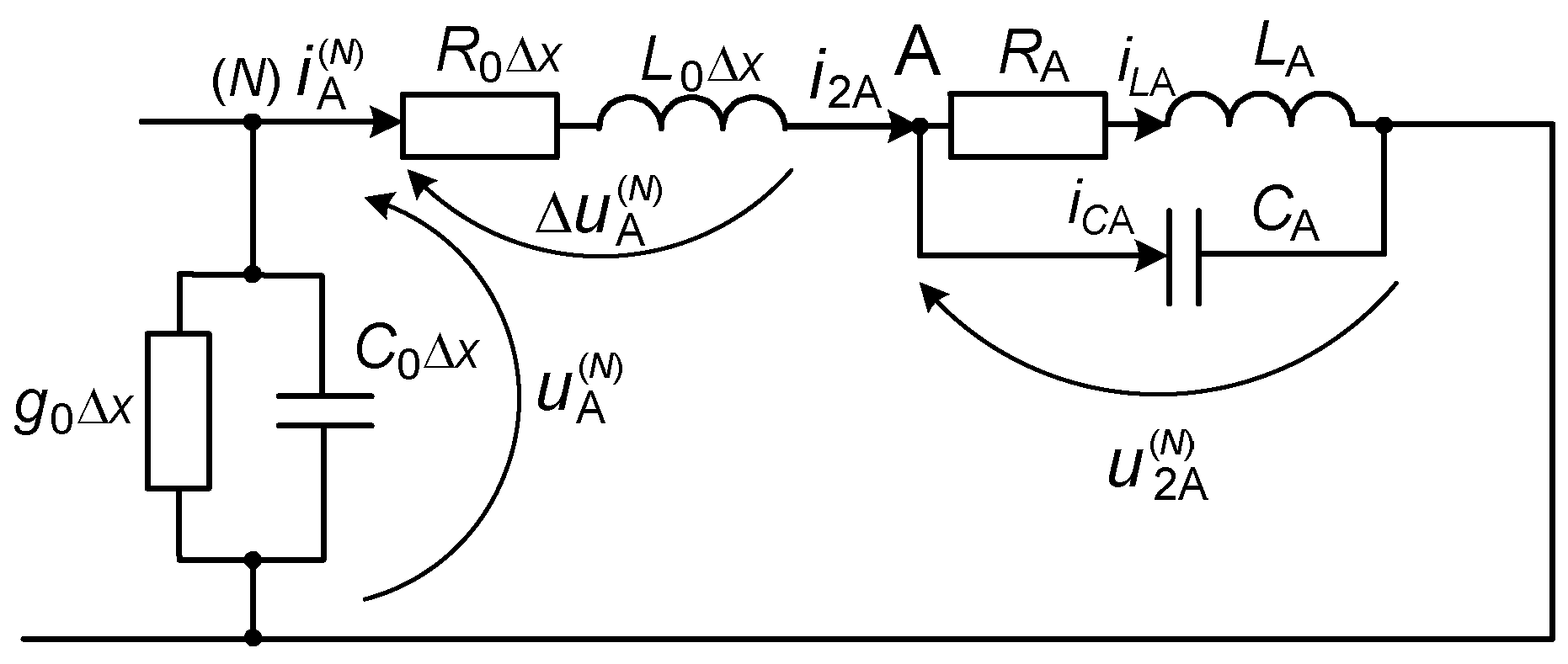
Experience shows that for solving problems of a similar type, it is recommended to use the transmission line equation, which is written as a function of the line voltage, i.e.,
λ ≡
u [
9,
26]. Let us present the phase A load for the transmission line (see
Figure 3).
Given
λ ≡
u, boundary conditions will be formulated for the transmission line Equation (41). The functions of the three-phase voltage system at the line’s beginning are specified. This means Dirichlet boundary conditions of the first type were used. The functions of the voltage system at the line’s end are unknown, on the other hand. Poincare boundary conditions of the third type will be applied in this case. Kirchhoff’s second law for distributed parameter systems will be written in the matrix–vector notation; see
Figure 1 and
Figure 2:
where
L—the length of the line.
Equation (41) for
λ ≡
u will be rewritten as a system of equations:
Equation (43) and the second expression in (42) will then be discretized using the straight-line method and considering the central derivative, as defined by:
where
n—the number of a discretization node in the integration space, that is, the line in this case. The following results are then:
where
n is the order of the discretization node,
N—the number of equation sampling units with respect to the spatial coordinate.
By analyzing Equations (45) and (46), it can be seen that when
n =
N, an unknown function
u(N+1) arises, which is the voltage at the blind (fictitious) sampling node. This voltage is commonly virtual and of merely mathematical significance. The basic idea for the continuing solution to the system of equations is now to find the voltage as the necessary stage of modeling the system in
Figure 2 and
Figure 3.
On the basis of the schematic diagram in
Figure 3, the following equations will be written in the matrix–vector notation:
Equating (46) and (48) and considering the first expression in (47) will produce:
Considering the second expression in (47), the equation for
uC will be written in line with the definition:
where, cf. (47):
where
The currents across the three-phase power supply line are sought by spatial sampling of the second equation in (42) using the straight-line method, but for this purpose only the right-side derivative of the function with respect to the spatial coordinate is used as defined below.
According to Kirchhoff’s second law, the equation for a distributed parameter power line will be written as:
The discrete form for the n-th circuit of the equivalent line, see (54), will be as follows:
where
i*(n)—currents in the line discretization units.
Equation (51) serves to compute i(N) in (50). This can give rise to the question of why these currents cannot be calculated based on (55) for n = N, cf. (56). The point is, (56) is a result of (55) by discretizing with the right-side derivative (see (54)), while (45) results from (46) by means of the central derivative, cf. (44). Therefore, integration in a sole system of discrete equations using different discretization types will be incorrect. The results of (56) are not employed in calculations and are of a purely informative nature.
Equations (45), (46), (50)–(52), and (56) are integrated jointly, considering (13), (40), (47), and (53).
3. Results
A computer simulation is undertaken to study transient electromagnetic processes in the power supply system. A simplified system diagram is shown in
Figure 3, where the power line is connected to an asymmetrical load. Once a steady state is reached, a single-phase short-circuit occurs at point A at the line’s end. The line is turned on considering the specific nature of controlled switching; in particular, the line is switched on at such a time instant that the instantaneous phase voltage is zero. Once the system becomes stabilized at t = 0.08 s at the line’s end in phase A, a single-phase short-circuit to the earth is simulated in point A.
The parameters of the calculation diagram in
Figure 3 correspond to those of a real 750 kV, 476 km-long power supply line between the West Ukrainian switch station (Ukraine) and Albertirsha (Hungary). These are the parameters of the long power line:
R0 = 1.9 × 10
−5 Ω/m,
L0 = 1.665 × 10
−6 H/m,
C0 = 1.0131 × 10
−11 F/m,
g0 = 3.25 × 10
−11 Sm/m,
C = 1.0122 × 10
−12 F/m,
g = 3.25 × 10
−13 Sm/m,
RZ = 5 × 10
−5 Ω/m,
M = 7.41 × 10
−7 H/m. Equivalent load parameters are assumed, so that the power factor when transmitting energy is 0.95:
RA = 420 Ω,
RB = 350 Ω,
RC = 310 Ω,
LA = 0.82 H,
LB = 0.75 H,
LC = 0.63 H,
CA = 0.000002 F,
CB = 0.0000018 F,
CC = 0.0000015 F. Computer simulation is conducted for the following voltages:
eA = 615 sin(
ωt) kV,
eB = 615 sin(
ωt − 120°) kV,
eC = 615 sin(
ωt + 120°) kV.
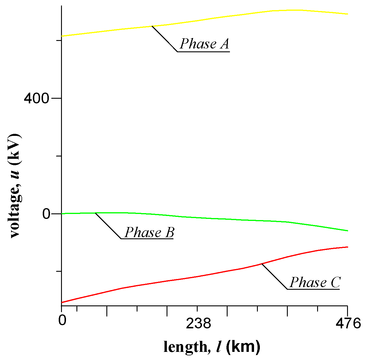
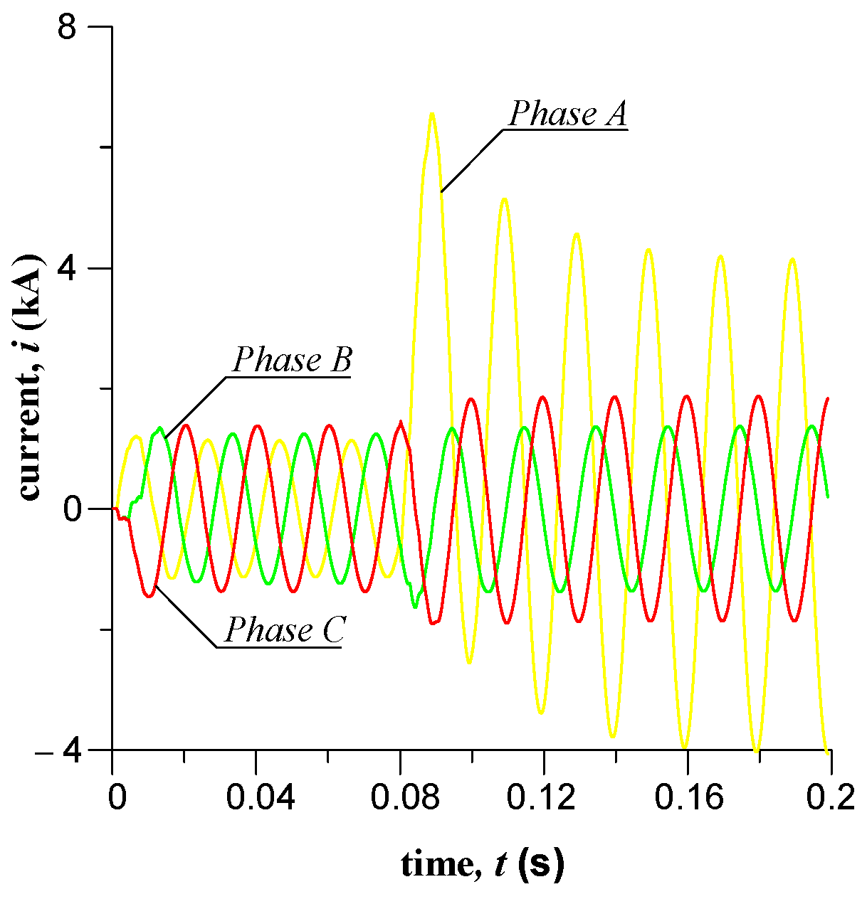
The voltage and current waveforms in the Figures are colored as follows: phase A—yellow, phase B—green, phase C—red.
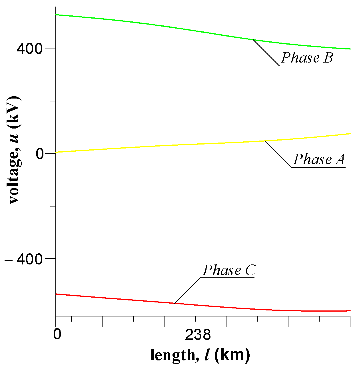
The phase voltage across the line as a function of distance at
t = 0.005 s from the time of the voltage turn-on is depicted in
Figure 4.
We can see that at t = 0.005 s, the phase A voltage at the line’s beginning is 600 kV, rising gradually along the line until reaching 640 kV. The phase B voltage at the line’s beginning is zero and rises gradually along the line until reaching −40 kV due to the presence of mutual inductances. The phase C voltage at the line’s beginning is −300 kV, to diminish gradually and reach approximately −100 kV at the end of the line.
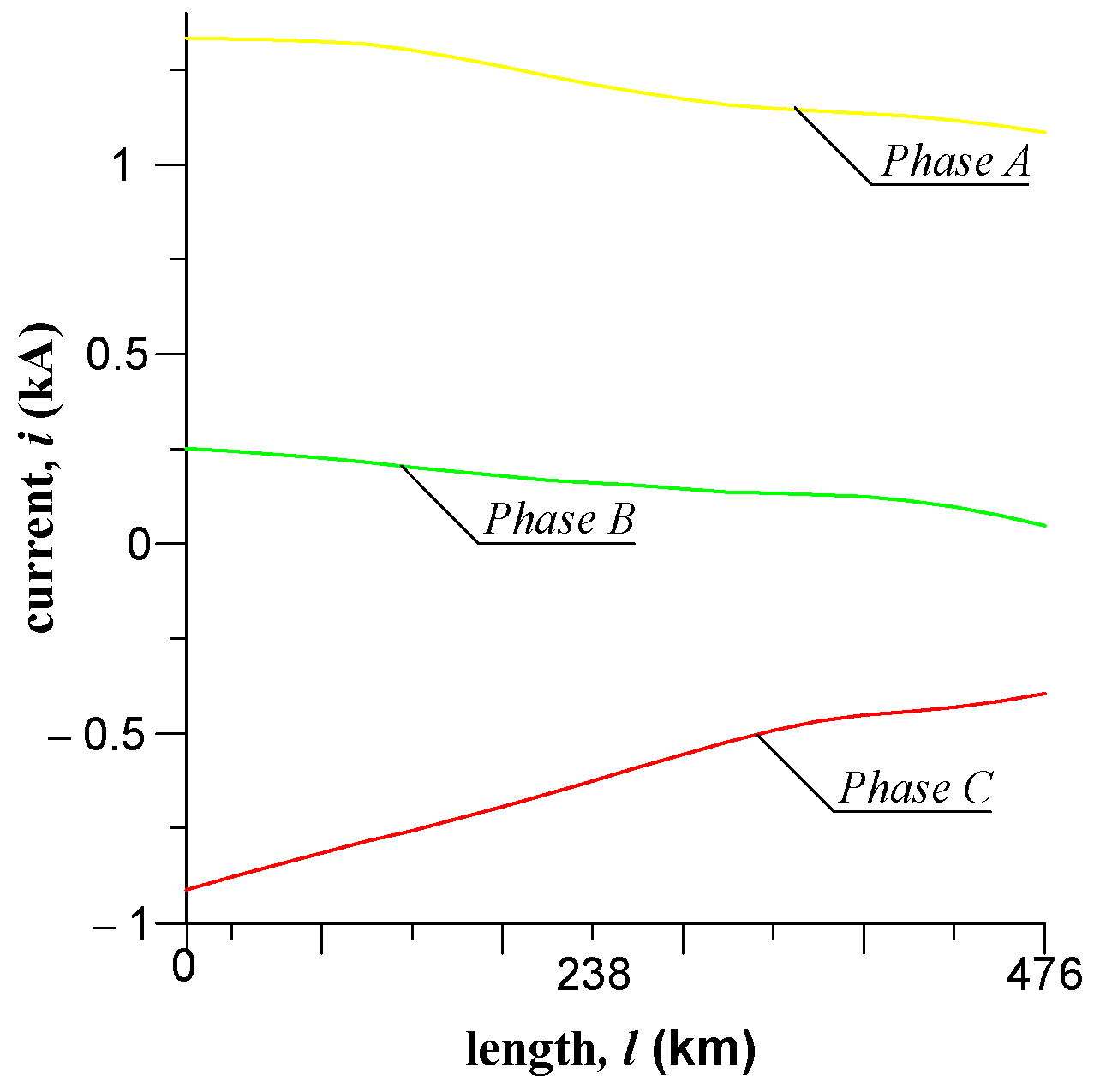
The phase current across the line as a function of distance at
t = 0.005 s from the time of the voltage turn-on is depicted in
Figure 5.
We can see that at t = 0.005 s, the phase A current at the line’s beginning is 1.7 kA, diminishing gradually along the line until reaching 1.2 kA at its end. Since phase B is not yet on at t = 0.005 s, the phase B current is induced from phases A and C and is nearly linear; it is up to 250 A at the line’s beginning and almost zero at its end. The phase C current at the line’s beginning is −800 A and −300 A at its end.
The phase voltage across the line as a function of distance at
t = 0.01 s from the time of the voltage turn-on is depicted in
Figure 6.
At
t = 0.01 s, the voltage (
Figure 6) and current (
Figure 7) vs. distance are nearly linear since, by then, electromagnetic waves were running repeatedly along the line to its end and back many times at identical parameters.
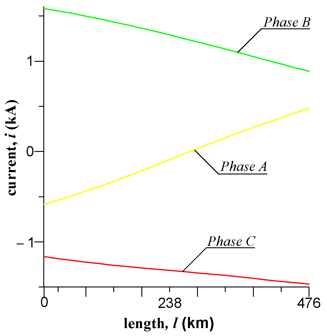
The phase current across the line as a function of distance at
t = 0.01 s from the time of the voltage turn-on is depicted in
Figure 7.
As in the case of the voltage, the phase current vs. distance at t = 0.01 s is close to linear since, by then, electromagnetic waves were running repeatedly along the line to its end and back many times at identical parameters.
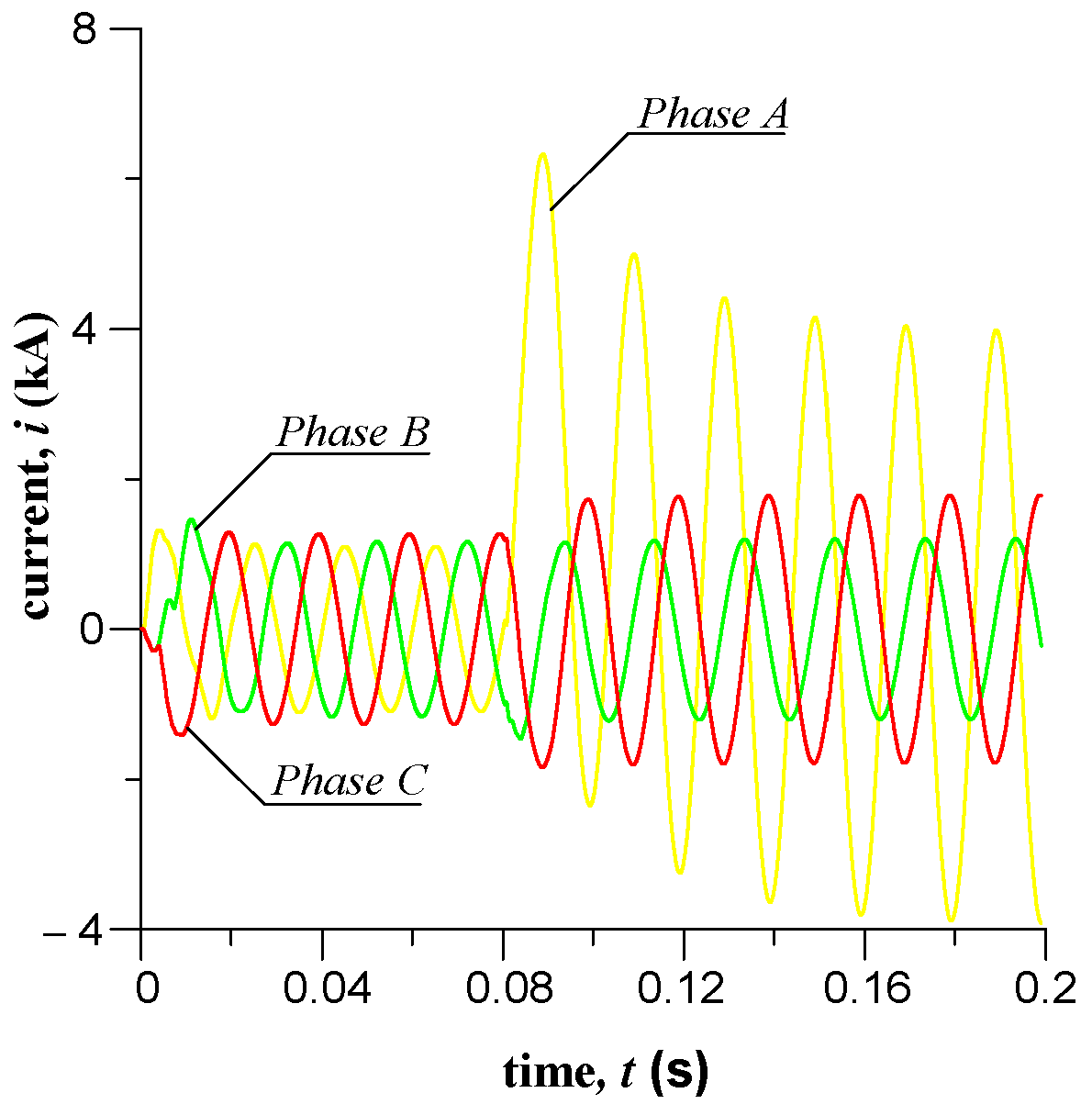
Figure 8 shows phase current waveforms when the line is on and then switches at
t = 0.08 s to a state of single-phase short-circuit fault at point A at the end of the line.
Since the load of the power supply line is unbalanced, the phase current amplitudes in the steady state have different values. For example, in the middle of the line, the current amplitude for phase A is 1 kA, for phase B it is 1.1 kA, and for phase C it is 1.3 kA. After a single-phase short circuit occurs at point A at the end of the line, at the time t = 0.08 s from the moment of switching on the voltage, the surge current of this phase in the middle part of the line reaches 6.25 kA, and the current amplitude in the steady state is 4 kA.
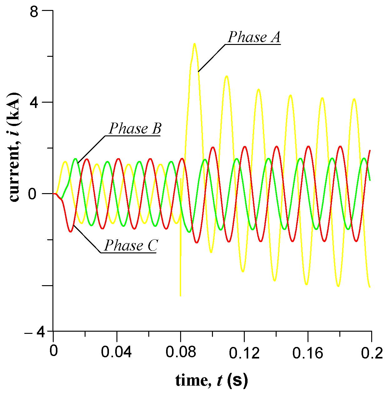
Figure 9 shows the waveforms of the phase currents at the end of the line when it is on and then switches at
t = 0.08 s to the single-phase short-circuit at the end of the line at point A.
Analyzing the current waveforms at the end of the line, we see that the steady-state amplitude of the C phase current during normal operation is 1.7 kA, while following a phase A short-circuit fault, the C phase current amplitude increases to 1.9 kA, and the B phase current amplitude practically does not change.
The current waveforms across the load branches are nearly the same as the current waveforms at the line’s end, cf.
Figure 9 and
Figure 10.
Controlled line switching is simulated in this study; therefore, surge currents are virtually absent as the line is turning on (see
Figure 8,
Figure 9 and
Figure 10).
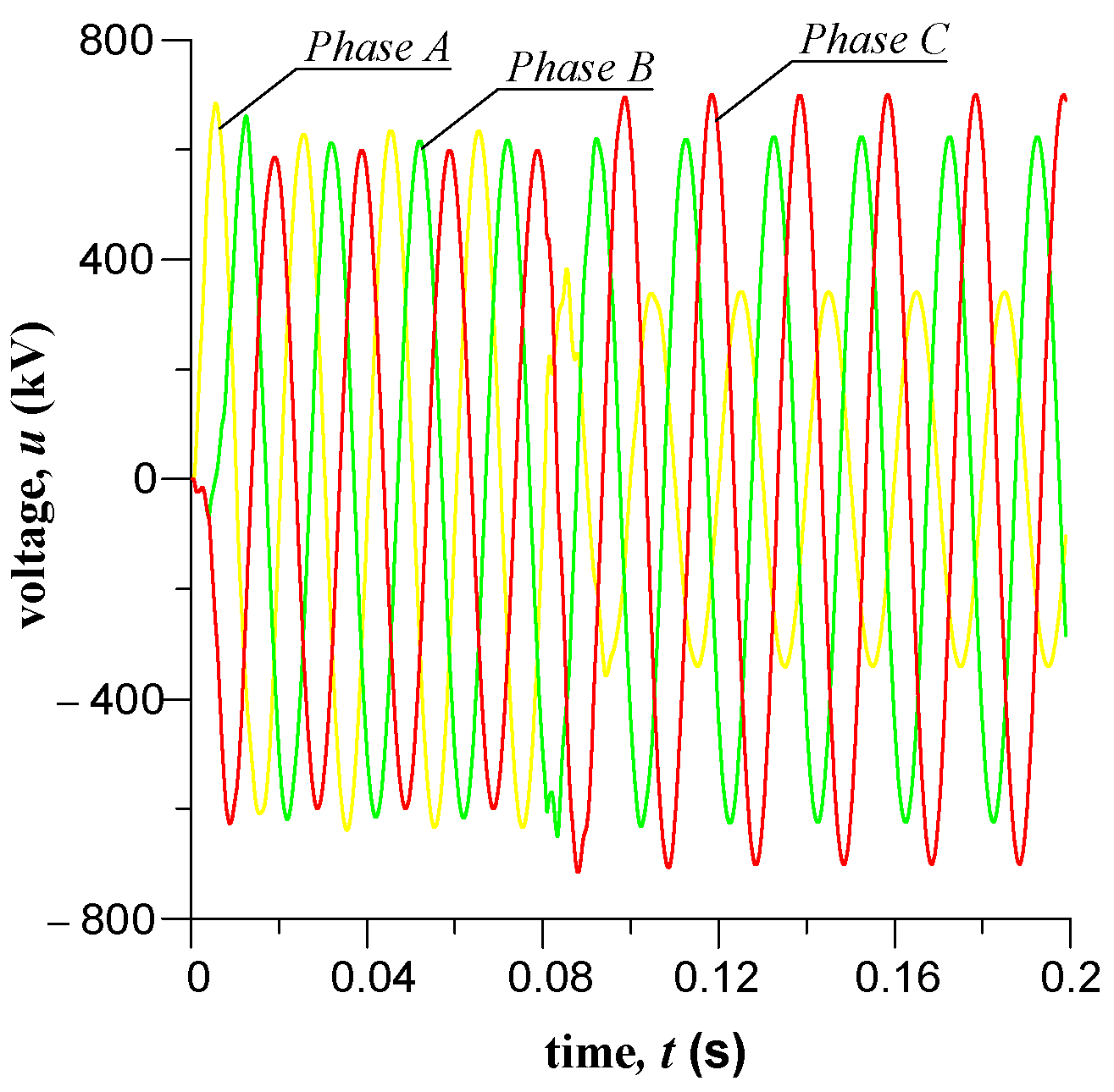
The phase voltage waveforms in the middle section of the line, presented in
Figure 11, show that the amplitudes of these voltages in the steady state of the system are as follows: A—620 kV, phase B—610 kV, phase C—600 kV.
The phase voltage amplitudes change following a short-circuit: for phase A, the voltage amplitude decreased to 330 kV, for phase B, it changed slightly, and for phase C, it increased to 700 kV.
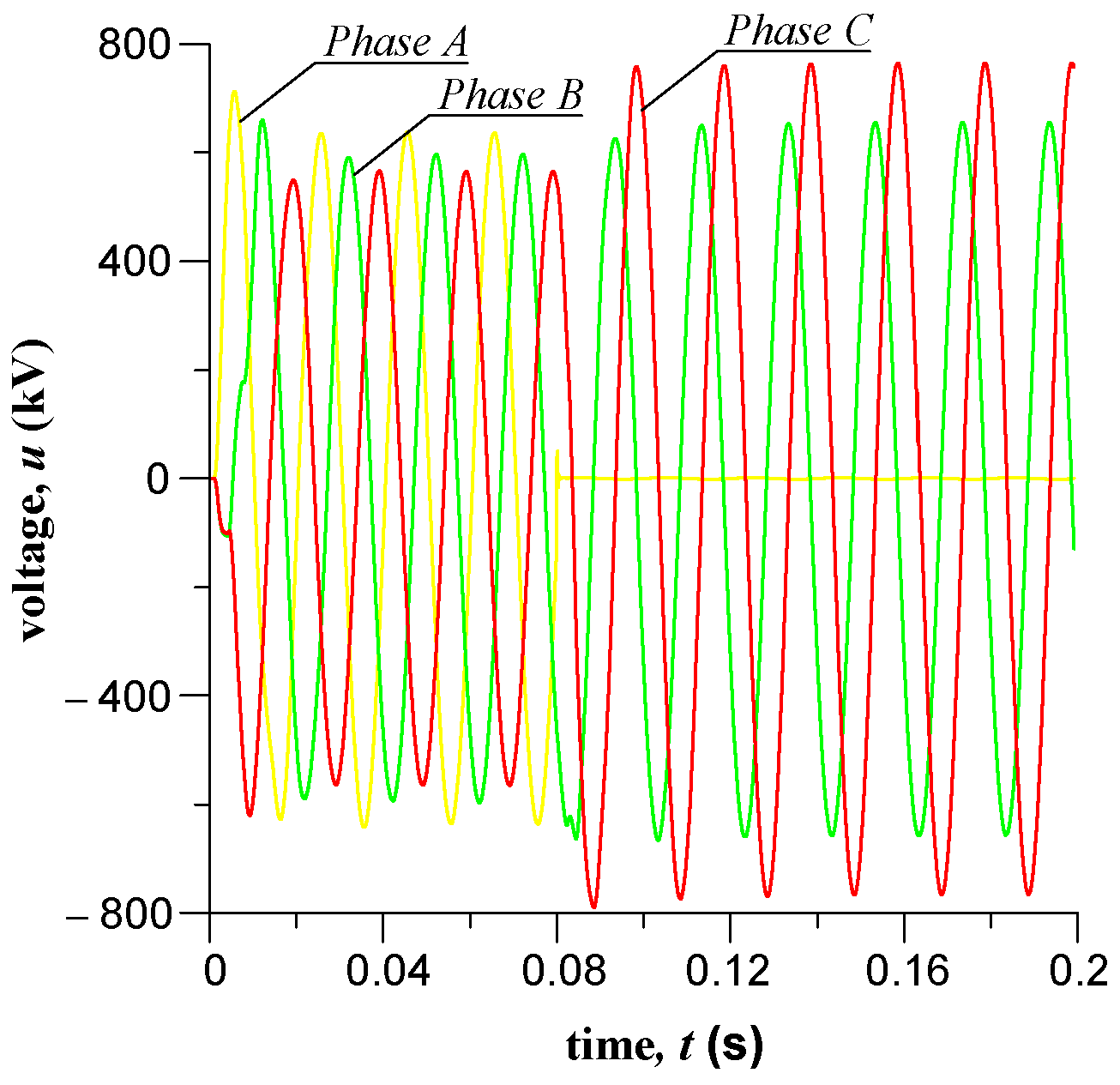
The values of phase voltages at the end of the line as presented in
Figure 12 suggest that under normal operating conditions, the voltages in all the phases are comparable.
However, as a result of the short circuit fault, the voltage amplitude of phase A decreased to zero, for phase B, it increased to 650 kV, and for phase C, it increased to 780 kV.
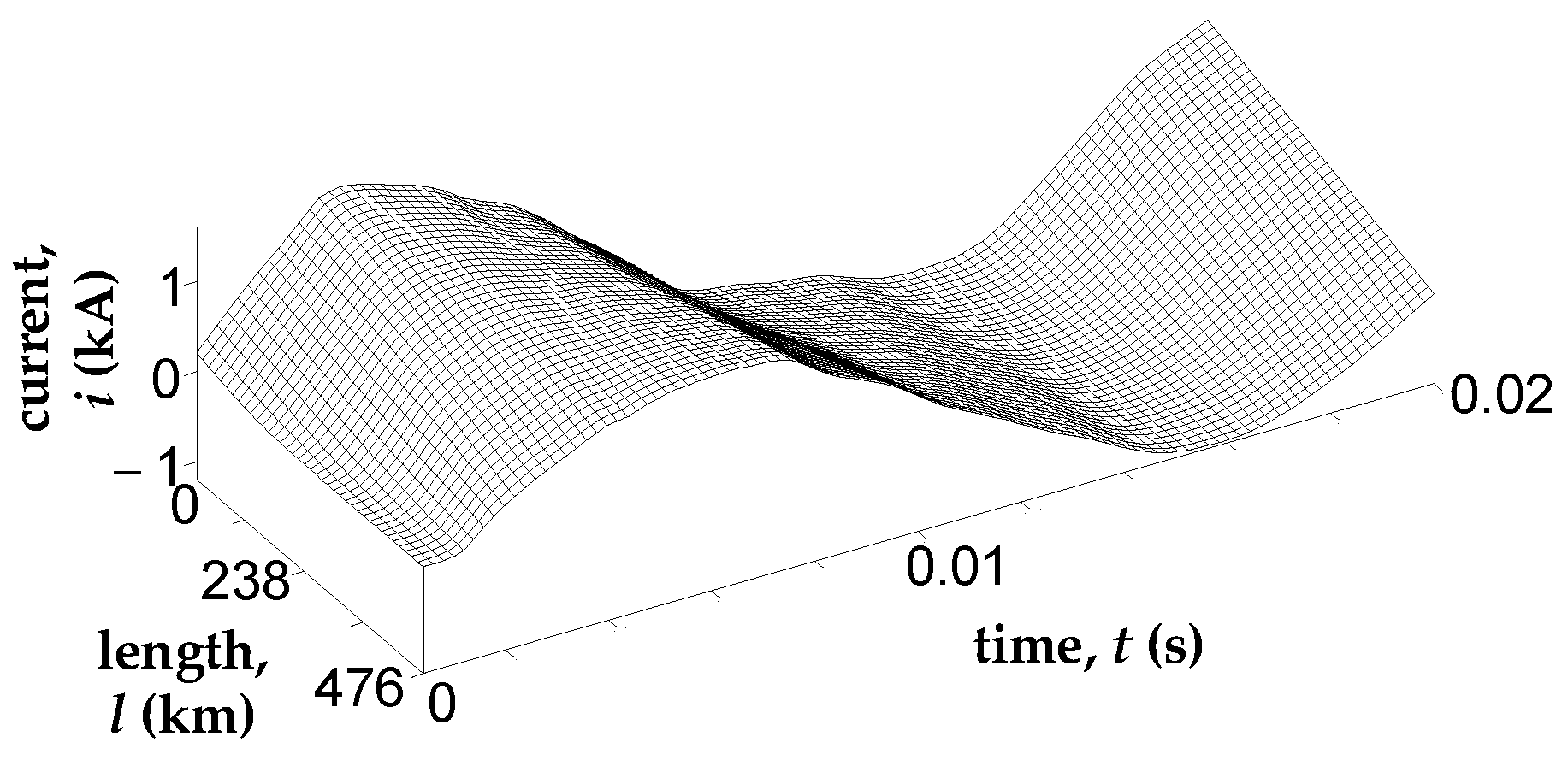
Figure 13 contains a temporal–spatial waveform of phase A current in the time range
t ∈ (0; 0.02) s.
Reasons for the shape of the current waveform can be found by analyzing the electromagnetic wave’s motion. Transient processes can be analyzed on the basis of the temporal–spatial current waveform from the perspective of the electromagnetic field.
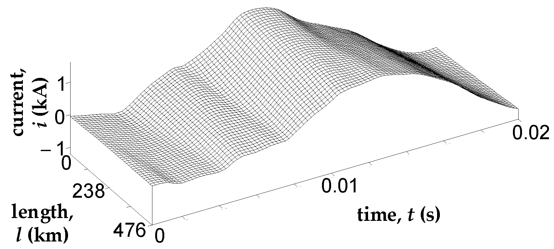
Figure 14 includes a temporal–spatial waveform of phase B current in the time range
t ∈ (0; 0.02) s.
Figure 14 indicates that phase B current, before energizing this phase, is very low, but above zero. This is related to the phenomenon of mutual induction.
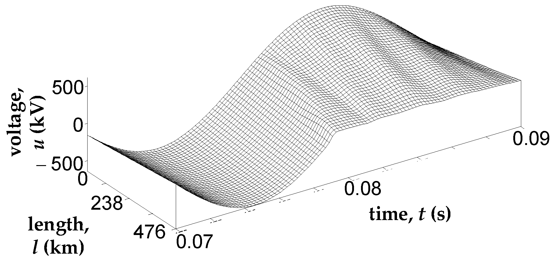
Figure 15 shows the temporal–spatial waveforms of phase A voltage in the time range
t ∈ (0.07; 0.09), which represents the short-circuit processes at
t = 0.08 s.
Since the end of the power line is short-circuited, the voltage (
Figure 15) is near zero, rising gradually towards the line’s start and adopting the values of the line supply voltage.
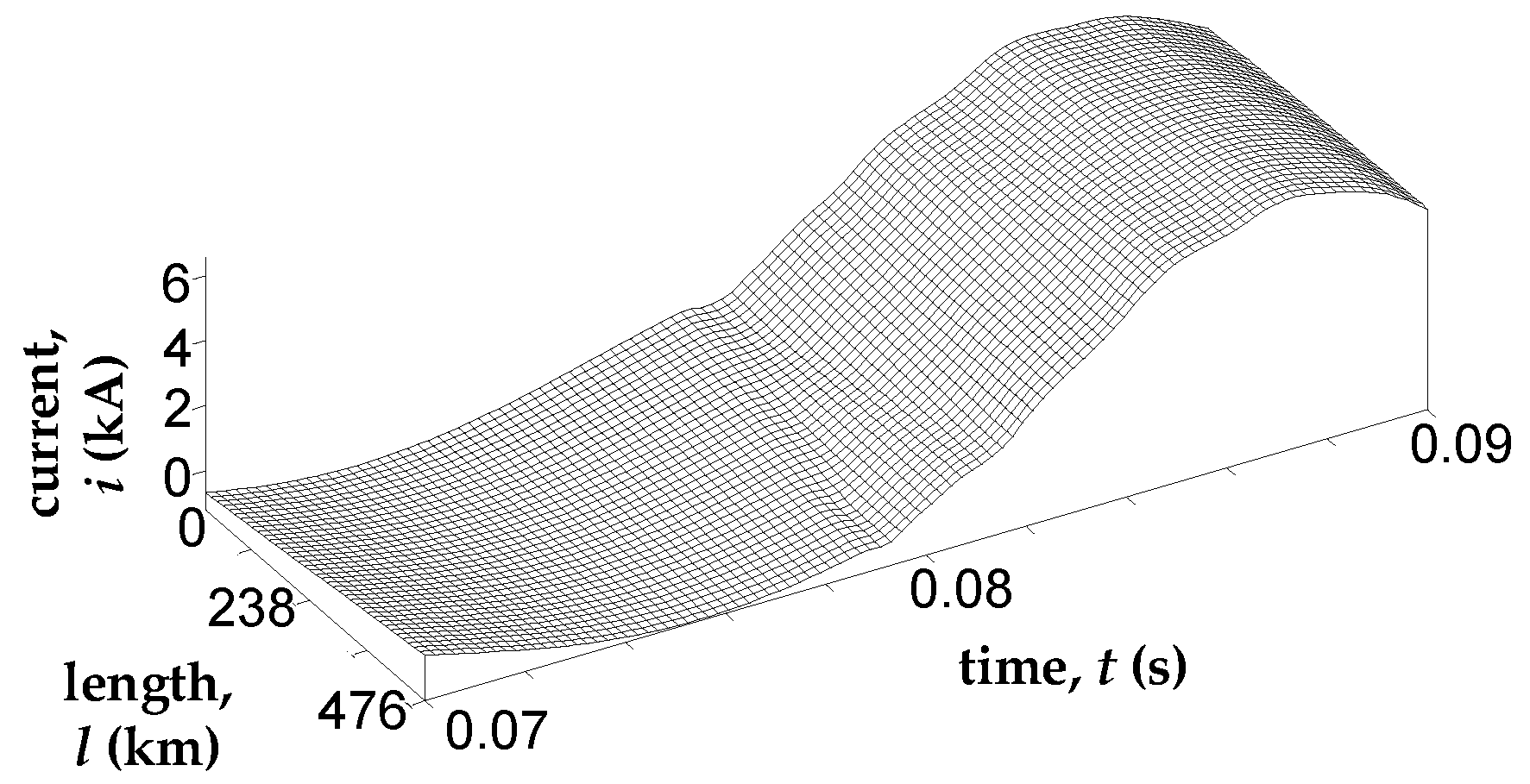
Figure 16 shows the temporal–spatial waveforms of phase A current in the time range
t ∈ (0.07; 0.09), which represents the short-circuit processes at
t = 0.08 s.
The situation is somewhat different in the case of phase A current (
Figure 16). It begins to rise from the line’s end and gradually changes all along the line. Then, its amplitude becomes nearly identical all along the line.
Based on the modified Hamilton–Ostrogradsky principle, a mathematical model is developed here of a three-phase power supply line with an unbalanced loading of an RLC circuit. Importantly, the equations of the three-phase line are fully consistent with the equations derived from field-based methods or classic approaches [
22,
27]. We stress that the concept of using variation approaches to produce a transmission line equation based on the Hamilton–Ostrogradsky principle has been long-known in the literature [
22]. The concept rests on the assumption, however, that there are no power losses across the line [
22]. By modifying the Hamilton–Ostrogradsky principle, we generate a real transmission line equation, fully consistent with the well-known equation of a three-phase line in its matrix–vectoral form derived from the classic approaches. What is crucial to the process of arriving at the line equation, the transverse loss matrix
G0, see (40), is determined purely analytically. This confirms the validity and competitiveness of variation approaches compared to classic approaches, made possible by modifying the Hamilton–Ostrogradsky principle. Starting from this, one can conclude that the ideology of expanding the Lagrange function for lumped parameter systems [
7] to the systems of distributed parameters [
10] is competitive in comparison with classic methods. Furthermore, the application of interdisciplinary variation approaches to some cases of modeling highly complex objects may be the only feasible solution.


