
Optimal Power Sharing in Microgrids Using the Artificial Bee Colony Algorithm


College of Electrical Engineering, Zhejiang University, Hangzhou 310027, China
*
Author to whom correspondence should be addressed.
Energies 2022, 15(3), 1067; https://0-doi-org.brum.beds.ac.uk/10.3390/en15031067
Submission received: 20 December 2021
/
Revised: 8 January 2022
/
Accepted: 19 January 2022
/
Published: 31 January 2022
(This article belongs to the Topic Optimisation, Optimal Control and Nonlinear Dynamics in Electrical Power, Energy Storage and Renewable Energy Systems)
Abstract
:In smart grids, a hybrid renewable energy system that combines multiple renewable energy sources (RESs) with storage and backup systems can provide the most cost-effective and stable energy supply. However, one of the most pressing issues addressed by recent research is how best to design the components of hybrid renewable energy systems to meet all load requirements at the lowest possible cost and with the best level of reliability. Due to the difficulty of optimizing hybrid renewable energy systems, it is critical to find an efficient optimization method that provides a reliable solution. Therefore, in this study, power transmission between microgrids is optimized to minimize the cost for the overall system and for each microgrid. For this purpose, artificial bee colony (ABC) is used as an optimization algorithm that aims to minimize the cost and power transmission from outside the microgrid. The ABC algorithm outperforms other population-based algorithms, with the added advantage of requiring fewer control parameters. The ABC algorithm also features good resilience, fast convergence, and great versatility. In this study, several experiments were conducted to show the productivity of the proposed ABC-based approach. The simulation results show that the proposed method is an effective optimization approach because it can achieve the global optimum in a very simple and computationally efficient way.
1. Introduction
Today, the world’s greatest challenges are the rapidly growing demand for electrical energy [1], rising electricity prices, the increasing use of non-renewable energy, the limits of conventional energy for power generation, global warming, global climate change, and related environmental problems [2]. All these challenges have resulted in the world being in a catastrophic economic and political crisis. Because of this, every government in the world is eager to expand renewable energy generation [3]. Renewable energy generation can help nations achieve their long-term development goal of providing safe, cheap, clean, environmentally friendly, and sustainable energy [4]. Despite the many advantages offered by renewable energy compared to conventional energy, they all have weaknesses in common, such as high weather vulnerability, low stability, and high unpredictability [5], all of which lead to low reliability and efficiency of energy generation [6]. Consequently, the hybrid renewable energy system can solve important problems and constraints in efficiency, reliability, and economy [7], which makes it an effective choice to meet the load requirements and support and improve the system [8]. The use of a central control unit to control the integrated power management of microgrids improves the efficiency, flexibility, and response time to fluctuations. The optimal power flow in the grid, the voltage level in each bus, and the transmission losses are all essential variables to be considered in efficient power systems [9]. The actual problem is an MILP problem, and the constraints on the optimal power flow are linear. For this purpose, a stochastic two-stage model of the interactions between the distribution system operator and many microgrids on the distribution line is used in [10].
The Stackelberg game concept is used in [11] for the interconnections between generators and microgrids. This model considers all electrical power flow constraints, voltage constraints, and line losses. The main objective of each is to maximize the profit.
MGs are classified in terms of power, control, mode, phase, and applications, as shown in Figure 1.
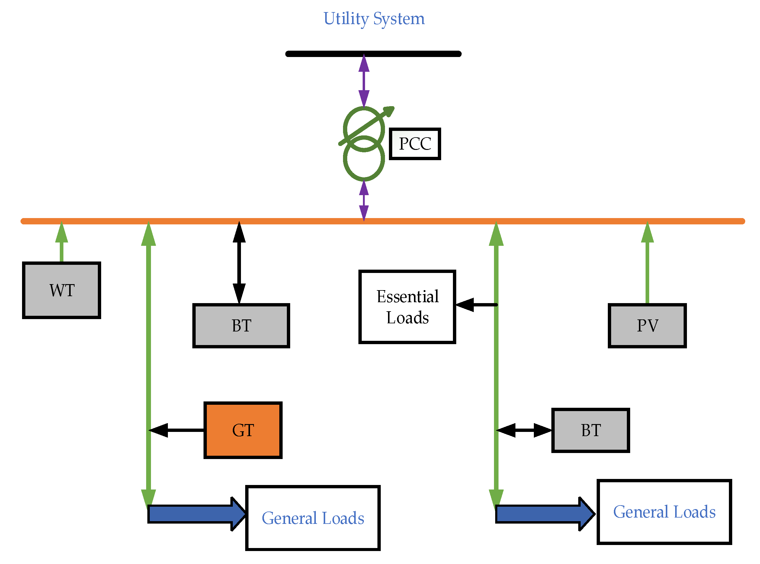
A microgrid (MG), as shown in Figure 2, consists of various distributed energy sources (DERs), responsive loads, and critical loads. A common connection point (PCC) connects the MG to the main grid [12]. Each DER is connected to the power electronic interface (PEI) in both grid-connected and islanded modes to perform control, measurement, protection, and plug-and-play functions. An MG in the grid-connected mode benefits from sharing power with the main grid. However, in the event of a fault or failure of the main grid, MG switches to the islanded mode to ensure system stability. In this mode, critical loads are continuously supplied with power by efficiently integrating DERs, demand response (DR), and load shedding (LS). The central microgrid controller (MGCC) and local controllers (LCs) manage and coordinate the entire MG operation [13]. Efficient DER management and coordination in MG lead to higher system performance and long-term development [14]. Due to increased environmental awareness, socioeconomic growth, and the need to reduce greenhouse gas emissions, MGs are mainly composed of sustainable energy systems, such as renewable energy sources and energy-efficient systems that use local heat waste [15]. Various energy storage technologies that have potential for high penetration and integration in microgrids are mentioned in [16]. Different energy trading systems are examined for interactive energy trading, multienergy management, and resilient operations in [17]. The DSM technique is used in [18] to reduce the operating cost of the grid-connected microgrid. An optimization-based energy management system is used to reduce the generation and curtailment costs [19]. In [20], an optimization controller is developed to control the energy management system for distributed energy sources in microgrids.
Table 1 shows a few examples of sustainable energy being used to run the energy management system from the literature review.
The microgrid EMS is a decision-making technique. For sustainable development, these techniques improve system efficiency, boost system reliability, decrease energy consumption, reduce DER operating costs, decrease system losses, and eliminate GHG emissions.
This paper presents a model for a hybrid renewable energy system integrated with a smart grid. The hybrid system includes wind turbines (WTs), photovoltaic (PV) systems, an electricity distribution company (Disco), gas turbines (GTs), and battery storage. Each component of the generation and load side is represented by a model. The hourly data of the wind speed and solar radiation on a daily basis are used as a case study in this paper. The proposed approach is used to optimize the power-sharing in the MGs to minimize the total cost of the system and the cost of each integrated microgrid. An artificial bee colony (ABC), as the optimization algorithm, is designed here to deal with the proposed model, with the objective of minimizing the cost and power imported from outside the MG. The idea of this paper is represented in Figure 3.
Figure 3 shows a microgrid (MG) connected to a distribution network. This MG contains multiple small MGs, which are connected with each other by electric lines. The electric line can be allowed to export and impart energy from small MGs. The small MG contains a mixture of components that consume and produce electricity (solar and wind plants) in addition to electricity storage units. The operational status of the small MG is divided into three sections: first, self-sufficiency in the event of equal production and consumption, so the MG will neither import nor export energy; second, import, which occurs when consumption is greater than production, as the MG needs energy; and third, export, which occurs when there is a surplus of energy within the MG and it needs to be exported.
Optimization is a mathematical problem that may be found in all engineering domains. This term’s literal definition is “best possible or desirable”. Because optimization problems are so broad and varied, it is a significant academic field.
Optimization algorithms are classified into two types: deterministic and stochastic. Previously, tackling optimization issues required tremendous computational effort, which frequently failed as the problem size grew larger. This is why bio-inspired stochastic optimization algorithms are being used as computationally efficient alternatives to deterministic approaches. Metaheuristics are based on the iterative improvement of either a population of solutions (evolutionary algorithms or swarm-based algorithms) or a single solution (Tabu Search) to solve a given optimization problem, and they primarily use randomization and local search.
The literature on bio-inspired algorithms (BIAs) for solving a wide variety of issues is vast, and various studies have reported on the usefulness of such tactics for handling difficult problems in the main disciplines of engineering in recent years. The two most prevalent and successful BIA classes or routes are evolutionary algorithms and swarm-based algorithms, both inspired by animals’ collective behavior and natural development. In order to obtain a broader view on the subject, the algorithms were divided into regions based on where the inspiration for them came from in nature.
Swarm intelligence is a novel and rising paradigm used for creating adaptive systems in bio-inspired computing. In this sense, evolutionary computation (EC) is an extension of this. Swarm intelligence is based on organisms’ collective social behaviors, whereas evolutionary algorithms are based on species’ genetic adaptability. Swarm intelligence, as defined in the literature, is the use of the collective intelligence of groups of simple organisms to solve problems, based on the behavior of actual insect swarms. The term “swarm” refers to the chaotic movement of particles in the affected region. Some important SI algorithms are particle swarm optimization (PSO), the ant colony optimization algorithm (ACO), the fish swarm algorithm (FSA), the firefly algorithm, and the artificial bee colony (ABC) methods, which have all been employed as optimization methodologies. In the foraging process, these algorithms, which were inspired by animals’ collective behavior, exhibit decentralized self-organized patterns. However, the artificial bee colony (ABC) approach was used in this article [32].
The ABC algorithm outperforms or is similar to other population-based algorithms, with the added advantage of requiring fewer control parameters. The ABC algorithm also features good resilience, fast convergence, and great versatility.
The ABC algorithm, developed by Karaboga and Basturk, replicates the intelligent foraging behavior of a honeybee swarm. The ABC algorithm’s artificial bee colony is made up of three categories of bees: hired bees, bystanders, and scouts. An employed bee is a spectator who does not participate in the dance but instead travels to the food source being frequented by the observer. The scout bee, on the other hand, performs random searches for fresh sources. The quality (or fitness) of a solution may be measured by comparing the location of a food source to the amount of nectar it generates. Beehives are built and then released into the two-dimensional search space. Bees build social relationships with one another while foraging for nectar. Intense bee–bee interactions are essential to the discovery of a solution.
2. Problem Formulation
2.1. ABC Algorithm
In 2005, Karaboga discovered the ABC algorithm, influenced by honey bee behavior. The algorithm of a honey bee colony has the ability to find the best quality food sources in nature with ease. Therefore, the concept of ABC was derived from the clever foraging behavior of honey bees to find suitable solutions to optimization problems. Generally, bee colonies are classified into three types according to their foraging ability: employed bees, onlooker bees, and scout bees. The employed bees are responsible for collecting nectar (food). They investigate the location of the food supply in advance and alert the scout bees about the quality of the food. Based on the information relayed by the employed bees, the scout bees wait in the swarm and decide whether to take advantage of a food source. The scout bees randomly search the environment for a new nectar supply, either from internal motivation or from likely external cues [33]. The quality (fitness) of the feasible solution to the optimization questions is related to the profitability of a nectar source. The presence of a nectar source indicates a feasible solution to the optimization issues. Each nectar source is visited by only one honey bee. In other words, the number of employed or onlooker bees is proportional to the number of nectar sources [34]. Employed bees maintain an excellent solution, onlooker bees accelerate convergence, and scout bees improve the ability to eliminate local optimums [35,36].
ABC Algorithm Iteration Steps
1. Initialization. Generate N random solutions (food sources) in a dimensional searching space D, where N represents the number of food sources, which is half the size of the colony is a D-dimensional solution vector. For the food source in the original population, and the number of optimization population parameters is denoted by D.
2. During the honey collection stage, each employed bee creates a new nectar source in the food source’s vicinity. When a new nectar source is compared to the previous one, the high probability will be memorized. Each onlooker bee assesses the attractiveness of nectar sources received from all employed bees and selects a food source with a high probability. Like the employed bees, she changes the source location in her memory and maintains a higher nectar supply. In these two phases, the following formula is employed to regenerate nectar sources:
where and is a random number that determines the generation range of neighborhoods. As the search comes closer to an optimal solution, the number of neighborhoods available will decrease.
3. Food source selection. In the next step, the onlooker bees compare the probability calculated by the fitness value to select a food source. Nectar sources with a high probability are chosen with a high degree of certainty. The chance of being chosen for food sources is computed using the equation below:
The fitness value of the solution may be determined using following equation:
If the quality of the new food source location is the same as or better than the previous one, the old one is updated with a new one, where is the value of the objective function for which is unique to the optimization problem. Otherwise, the old one will be kept the same as the stage of employed bees.
4. Population elimination. A solution is considered to have fallen into a local optimum solution if it has not improved significantly after a specified number of trials, known as “max iteration”, and the starting position is abandoned. As a consequence, the matching employed bees will become scout bees, and a new solution, which may be described as follows, will be generated at random in place of the discarded solution:
where and are the jth and ith individual maximum and lowest values, respectively, and and are the same (1).
3. Mathematical Modeling
The microgrid architecture studied in this paper is represented in Figure 5. It includes wind turbines (WTs), gas turbines (GTs), photovoltaic (PV), batteries (BT), additional storage components, general loads, and essential loads with different characteristics. The connection point, also known as the point of common coupling (PCC), is the interface between this architecture’s utility and microgrid systems. As a result, there are two types of modes.
When the MG is connected to the main grid via PCC, it is in the grid-connected mode, and when it does not connect with the main grid, it is in the islanded mode.
Renewable energy sources (RESs) can be connected via a DC, AC, or a hybrid DC/AC bus. For most generators and loads, the appropriate configuration is determined by the type of output power. Therefore, DC bus coupling is preferred when both loads and generators are DC [40]. When the loads and generators are AC, then AC bus coupling is preferred [41] when the generation and load are mixed, such as AC and DC hybrid renewable energy sources (HRESs). A hybrid AC, DC bus coupling system is used [42], as shown in Figure 6.
3.1. Hybrid Wind/PV/Battery Storage/Gas Turbine
The configuration shown in Figure 6 consists of wind energy, a PV energy system, battery storage, a gas turbine, and the main load. The response of this configuration is simple and easy to understand. Due to the bidirectional converter, the WT and the PV system are mainly responsible for supplying the main load. The excess power generated by wind and/or PV is stored in a battery storage system until the battery is fully charged to . Excess power generated above is supplied to dedicated loads, i.e., dummy loads, such as loads for cooling, home appliances and heating, and charging the batteries of emergency lights when the battery storage is full. When the load power exceeds the generated power, the batteries are used to make up the difference until they reach the minimum (). Suppose the battery is fully discharged by and the hybrid renewable energy sources cannot meet the microgrid’s load demand. In this case, it imports energy from another microgrid. Moreover, when it is unable to purchase energy from another microgrid, the microgrid purchases power from the main grid to balance the load demand [43].
3.1.1. Wind Energy System
Wind generation depends on both the wind speed and the height of the hub at a given location. The power–law equation [44] is used to calculate the wind speed at the hub height of WT using data collected at the anemometer height: and are the wind speeds at the hub height and the anemometer height , respectively, and is the roughness factor. The value changes from location to location and over time at the same location:
where and are the wind speeds at hub height and anemometer height . α is a roughness factor and varies from location to location and time to time.
The output power of WT from the typical WT curve is as follows [45]:
where is the output power of the wind turbine, is the rated output power of the wind turbine, is the cut in wind speed of WT, is the rated wind speed of WT, and is the cut off wind speed of the wind turbine.
3.1.2. PV Energy System
The solar radiation on a tilted surface can be calculated using solar insolation, the ambient temperature, data from the PV panel manufacturer, the PV panel slope, and the site latitude and longitude [46,47]. The following equation [48] is used to compute the PV system’s output power:
where is the PV system’s hourly generating efficiency, which may be calculated in terms of the cell temperature using Equation (8) [49]:
where is the temperature coefficient, and are the solar cell efficiency and temperature at maximum radiation solar flux , It is an hourly solar cell temperature at ambient temperature :
where (Ross coefficient) is a coefficient that represents how the temperature increases above ambient as solar flux increases. The overall output of the PV array is:
where is the PV array output power, is the irradiation of solar, is the solar irradiance under standard test conditions (). is the rated power of solar [49]. Table 2 represents the PV parameter values.
3.1.3. Battery Storage
The state of charge of a battery is determined based on the energy balance between the wind, PV energy systems, and the load as given by the following equations after a particular time (t):
where (11) is the battery charging mode equation:
where (12) is the battery discharging mode equation. is the energy of the battery bank, and is the charging and discharging efficiency of the battery storage system. It is considered to be 90% and 85%, respectively, in [50], where σ is the battery self-discharge rate and is assumed to be 0.2% per day for most batteries [51]. is the surplus power, and is the deficit power.
The battery bank should always follow the following limitations:
where and are the battery bank’s maximum and minimum storage capacity, respectively. The following equation can be used to calculate :
where is the battery nominal storage capacity, and DOD is the depth of discharge of a battery opposite to the SOC of a battery.
4. Mathematical Modeling of the Proposed Approach
The proposed approach of this article is to optimize the power transfer between microgrids to minimize the overall cost of the system and each microgrid. For this purpose, a mathematical model is designed for a net load for each microgrid first. The proposed idea is represented in Figure 3, and the proposed work is represented by the flowchart shown in Figure 7.
The proposed approach has two main tasks: storage; the other is energy sharing in the first part, which is energy storage. If the net load is greater than zero, storage is used to discharge energy to meet the load requirements. If the net load is less than zero, the extra system energy is either shared with other microgrids or stored in the storage system to reduce the total cost of electricity. Data about the load, PV, and wind in each MG is calculated. After obtaining data of the load, PV, and wind in each MG, the sharing parameters are initialized, such as the SOC of the battery, the size of the battery, and the minimum and maximum generation in each MG, the net load is calculated using the generation and load balance equations.
The proposed work shown in Figure 7 is about energy management in small MGs and is an attempt to reduce imports from energy distribution networks as much as possible, by linking several small microgrids together. These MGs contain different mixtures of energy production and consumption, which helps to increase the reliability of these small MGs and gradually dispense with power distribution networks. The novelty is that the difference in the energy mix between these small MGs and linking them together will help dispense with distribution networks, which will reduce energy losses and the price of electricity and provides the possibility for small consumers to benefit from the production and sale of energy.
Suppose a microgrid has a battery energy storage system. In this case, it will have two possibilities if the net load exceeds zero. The of a battery is checked to observe whether it is above 20%, and the battery will be discharged to meet the load requirements. Still, if the net load is not greater than zero, there is some extra energy in the system, which may be used to charge the battery if the of a battery is less than the maximum storage capacity.
In the second task of the proposed approach, whether the net load is greater than or less than zero is checked. If it is greater than zero, the microgrid will import energy from other microgrids or the main grid. If the net load is less than zero, the microgrid will export energy to other microgrids or the main grid.
The above process is iterated until optimal power-sharing among the microgrids is achieved.
4.1. Microgrids’ Net Load
The mathematical equation for Disco is:
where is the load of the distribution company (Disco) and is the conventional generation in Disco:
where is the load of , is the rated power of PV in , and is the 24 h PV profile:
where is the load of , , are the generation of conventional generators 1 and 2, is the wind turbine generation in , and is the wind profile of 24 h
is the load of , is the rated PV power, and is the PV profile for 24 h.
is the load of , is the wind turbine generation in , is the 24 h wind profile:
where is the load of , is the generation of a conventional generator, is the wind generation in , and is the 24 h wind profile.
The net load is the difference between the load and generation inside the MG itself. It is used to determine whether the microgrid has a shortage or excess of energy to import or export to other microgrids with a shortage of energy, store it in battery energy storage, or sell it to the main grid.
4.2. Energy Management Strategy
The proposed HRES management algorithm is described in the following strategy. If the amount of power generated by RES surpasses the amount needed to meet the load requirements, the excess power will be used to charge the batteries until they reach their maximum capacity, . The extra power in the batteries will be used to power the dummy load, . The reason behind this can be described as follows:
where is the power to the dummy load:
Equation (24) shows the charging process:
If the load demand requires more power than RES can provide, the battery will meet the demand until it is reduced to its minimal level. If there is still a power shortage, the DG will make up for the deficit load demand. The equations that describe this logic are as follows:
where is discharging power, and this is a discharging process:
All the above equations and details of the generation, load, and storage indicate how the energy management strategy is effectively working in this case. When the generation of HRES in the microgrid is higher than the load, the surplus energy is stored in the battery energy storage system. When the generation of the HRES is less than the load of the microgrid, then the shortage of energy is met by the battery storage system. If the generation of HRES is less than the load and the battery energy is less than the minimum level of stored energy, then the microgrid will import energy from another microgrid to meet the demand. In the above equations, is the state of the charge of the battery, is the power used to charge the battery, and is the discharging power of the battery. , is the battery charging and discharging efficiencies, respectively.
The power flow constraints of the HRES and battery are as follows:
4.3. Microgrid Energy Sharing Problem
The microgrid has an excess or shortage of energy. The microgrid with excess energy will export the energy to other microgrids, which need a power through-line between them The microgrid with a shortage of energy will import the energy from other microgrids, which have an excess power through-line between them . If all microgrids do not have enough energy to cover the shortage in the system, the system will import energy from the main grid. If we consider a sequence of , if sending end and receiving end , it means the line is connected from Disco to and so on.
5. Power Balance
The power balance in the generation and load is represented as:
Objective Function
The objective function is a cost reduction of the generated power, transfer power, and import and export power:
where is the total conventional generation cost, is the total transfer energy cost from Disco to , is the total transfer energy cost from , is the total energy cost from the battery, and is the penalty cost for the unsupplied energy.
Mathematically, all of the above costs are represented as:
where is conventional generation in Disco, is conventional generation in , is conventional generation in , is conventional generation in , and is the gas price:
where transfer power from Disco to , respectively, and is the energy cost of Disco:
where () is the power transfer from , and is the cost of energy from :
In Equation (38), is the energy of the battery in Disco, is the energy of the battery in , is the energy of the battery , is the energy of the battery in , and is the cost of energy from the battery:
where is the unsupplied energy and is the penalty price that is fixed [49].
6. Simulations and Results Analysis
As discussed above, in all the mathematical formulations regarding the objective functions and microgrid components, an ABC optimization technique reduces the system’s total cost and minimal sharing cost of all the microgrids. Microgrids consist of conventional generation and intermittent energy sources, such as PV, wind, and battery energy storage systems. Among all the sources, conventional generators produce 24 h electricity, and wind generation is wind speed dependent and PV dependent on solar irradiations. Conventional generation occurs in Disco, and . If their capacity fails to meet the desired load demands, they will import energy from the main grid if there is an unavailability of energy from other microgrids.
There are different power-through lines between Disco and microgrids and from microgrids to microgrids. The lines connecting Disco and microgrids are (), i.e., from . From the lines are (); from, the lines are (); from ; and the last connection between is . These lines from represent power transfer from Disco to and MGs to MGs. If the value of is negative, power is transferred from the receiving to the sending end and vice versa if it is positive.
A cost convergence curve is shown below in Figure 8, which shows how the best solution deals with each iteration. We can see the best solution decreases when the iteration increases until it reaches the best one. The maximum number of iterations considered in the proposed idea is 150, upon which it converges to an optimal value.
Regarding the MG with only PV generation source, Figure 9 shows that it can only generate power according to the solar irradiance data in the PVWT profile. For the rest of the hours, it imports energy from outside, and from 11 to 13 h, it sells energy as it exceeds the load demand. MG1 has only one PV generation source, and as per Equation (7), PV generation is dependent on thee tilted surface, PV array, and its efficiency. Maximum generation is achieved when maximum sunlight is available for the tilted surface, and it is generally from 7 to 19 h that power is generated. Moreover, the intensity of light is very high, from 11 to 13 h, during which the generated power reaches th maximum and is available to sell to other MGs or the main grid. In the absence of sunlight, MG1 will not generate electricity. Hence, it will purchase electricity from other MGs.
Microgrid 2 contains wind generation, battery storage, and 2 thermal units. The wind is almost always the available generation source, as shown in Figure 10. From 1–6 h, the load demand can easily be met by the wind generation source and thermal unit generation. During this time, extra power is used for charging the battery. From 7–8 h, EES is used to meet the load demand along with the wind and thermal generation sources. From 9–23 h, wind generation, thermal generation, and EES are not able to meet the load demand; hence, electricity is purchased from outside.
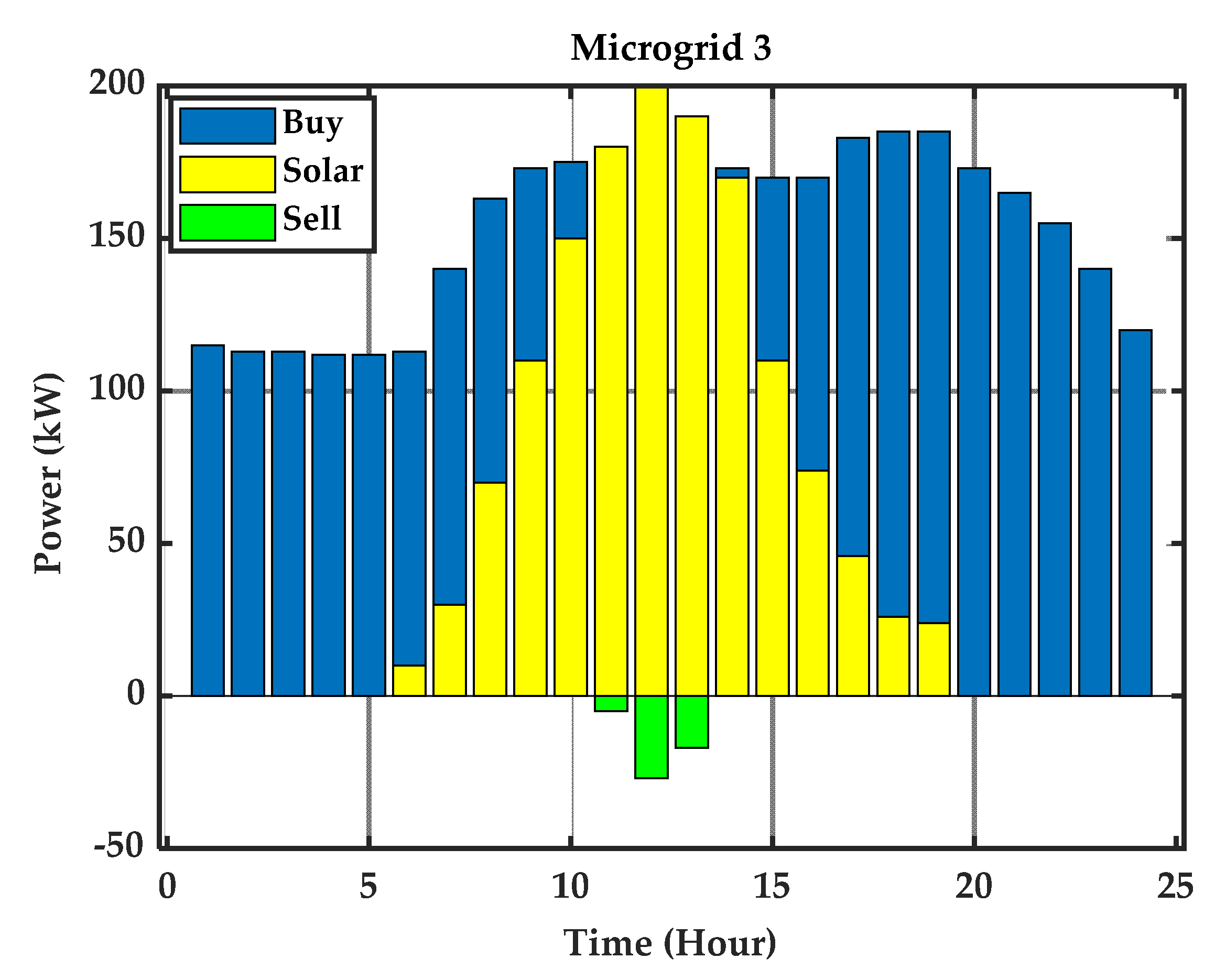
Microgrid 3 has one source of PV and load demand, as shown in Figure 11. To meet the load demand with just one PV source, it will purchase electricity from other microgrids in the absence of sunlight. When sunlight becomes available, it will gradually overcome the load demand and at high intensity, sunlight from 11–13 h MG3 will be able to meet the entire demand. The extra amount of electricity will be sold to other MGs.
MG4 contains wind generation and battery storage, and the load demand is shown in the Figure 12. The result in Figure 12 shows that from 1–6 h, wind generation is able to meet the required load demand and the extra amount of electricity will be used to charge the battery. Due to the intermittent nature of wind, it will purchase electricity if the wind generation is less than the load demand. As shown in Figure 12, from 7–10 h, the load demand exceeds wind generation; hence, EES is used to meet the load demand along with wind generation, and some energy is still required to meet the required demand, it will be purchased from other microgrids. From 11–24 h, wind generation cannot meet the required load demand; hence, the extra amount of electricity needed will be purchased from other microgrids.
MG5 contains wind generation, battery storage, and one thermal unit. The load demand is shown in Figure 13. Wind generation is available 24 h as shown in the figure. From 1–6 h, the load demand is met by wind and thermal generation and the extra amount of electricity is used to charge the battery. From 7–8 h, the load demand exceeds the wind and thermal generation; hence, EES is used to meet the required demand. From 9–24 h, as the load demand is higher than the inside generation, the extra energy required to meet the demand is purchased from other microgrids.
Disco contains battery storage and one thermal unit. The thermal generation is a constant source of generation as shown in Figure 14, and the load demand of Disco is shown in the figure. From 1–6 h, thermal generation alone cannot meet the load demand. Therefore, energy is purchased from other microgrids at the optimal rate and the battery is charged during this time. From 7–8 h, thermal generation and EES are both used, and the extra amount needed to meet the load demand is purchased from outside. From 9–24 h, thermal generation is used, but the generation is not sufficient to meet the required demand. Therefore, the extra amount is purchased from outside.
The cost optimization results of the microgrids and total systems are shown in Figure 15. It is clearly shown in the figure that the total cost of MG2, MG4, and MG5 is zero, which means that they do not import energy from other microgrids or the amount of electricity that is bought or sold is the same; hence, they compensate for their cost effects, which is why their cost is zero.
7. Conclusions and Future Work
The microgrid has emerged as a new paradigm shift for global energy systems to replace remote centralized power plants with more efficient, localized, and distributed generation systems, especially in various cities and towns around the globe. It provides more stable, flexible, and energy-efficient solutions for the power grid so that an increasing number of loads can be handled without new infrastructure needing to be built. This work provides a new iterative ABC optimization method that addresses HRESs, such as solar, wind, GT, and battery. In particular, this work optimizes the power transmission between different microgrids to minimize the cost of each microgrid and the whole system while maintaining the load requirements and stability. The optimization problem was solved by the new iterative method ABC. This study also conducted several experiments with historical data to test the proposed method for the HRES model. The simulation results show that the proposed method is efficient in finding the best solution and adjusting the optimization parameters and constraints. This method can also be applied to any site with meteorological data and any WT with technical information.
Future research will focus on the use of hybrid swarm intelligence systems, such as the particle swarm algorithm and the artificial bee colony algorithm or the differential evolution algorithm, for the economic dispatch of microgrids. In addition, flexible switching techniques for real-time scheduling in microgrids that consider more constraint situations is an interesting future research direction.
Author Contributions
Conceptualization, K.U. and Q.J.; methodology, software and validation, K.U. formal analysis, investigation and resources, R.A.K.; writing—original draft preparation, K.U.; writing—review and editing, G.G.; visualization, S.R.; supervision, Q.J. All authors have read and agreed to the published version of the manuscript.
Funding
This research received no external funding.
Institutional Review Board Statement
Not available.
Informed Consent Statement
Not applicable.
Data Availability Statement
The data that support the study’s findings, such as numerical simulation, model, or code generated or used during the study, are available upon request from the journal and the corresponding author.
Acknowledgments
Thanks to the China Scholarship Council, Zhejiang University, Hangzhou, China (www.zju.edu.cn, accessed on 18 January 2022) and the University of Science & Technology Bannu, Pakistan (www.ustb.edu.pk, accessed on 18 January 2022) for providing us great research environment during this work.
Conflicts of Interest
The corresponding author declares that there is no contradiction on behalf of all authors.
References
- Mohammed, O.H.; Amirat, Y.; Benbouzid, M.E.H.; Feld, G. Optimal Design and Energy Management of a Hybrid Power Generation System Based on Wind/Tidal/PV Sources: Case Study for the Ouessant French Island. In Smart Energy Grid Design for Island Countries: Challenges and Opportunities; Springer: Berlin/Heidelberg, Germany, 2017; ISBN 9783319501970. [Google Scholar]
- Child, M.; Bogdanov, D.; Breyer, C. The role of storage technologies for the transition to a 100% renewable energy system in Europe. Energy Procedia 2018, 155, 44–60. [Google Scholar] [CrossRef]
- Aslam, S.; Herodotou, H.; Mohsin, S.M.; Javaid, N.; Ashraf, N.; Aslam, S. A survey on deep learning methods for power load and renewable energy forecasting in smart microgrids. Renew. Sustain. Energy Rev. 2021, 144, 110992. [Google Scholar] [CrossRef]
- Zhang, D.; Mu, S.; Chan, C.C.; Zhou, G.Y. Optimization of renewable energy penetration in regional energy system. Energy Procedia 2018, 152, 922–927. [Google Scholar] [CrossRef]
- Stroe, D.I.; Zaharof, A.; Iov, F. Power and energy management with battery storage for a hybrid residential PV-wind system—A case study for Denmark. Energy Procedia 2018, 155, 464–477. [Google Scholar] [CrossRef]
- Zhou, Z.; Benbouzid, M.E.H.; Charpentier, J.F.; Scuiller, F. Hybrid Diesel/MCT/Battery Electricity Power Supply System for Power Management in Small Island. In Smart Energy Grid Design for Island Countries: Challenges and Opportunities; Springer: Berlin/Heidelberg, Germany, 2017; ISBN 9783319501970. [Google Scholar]
- Mohammed, O.H.; Amirat, Y.; Benbouzid, M.; Elbast, A. Optimal Design of a PV/Fuel Cell Hybrid Power System for the City of Brest in France. In Proceedings of the 2014 First International Conference on Green Energy ICGE 2014, Sfax, Tunisia, 25–27 March 2014. [Google Scholar]
- Zhang, J.; Huang, L.; Shu, J.; Wang, H.; Ding, J. Energy Management of PV-Diesel-Battery Hybrid Power System for Island Stand-Alone Micro-Grid. Energy Procedia 2017, 105, 2201–2206. [Google Scholar] [CrossRef]
- Khursheed, A.; Aslam, S.; Haider, S.I.; Mohsin, S.M.; ul Islam, S.; Khattak, H.A.; Shah, S. Energy forecasting using multiheaded convolutional neural networks in efficient renewable energy resources equipped with energy storage system. Trans. Emerg. Telecommun. Technol. 2019, e3837. [Google Scholar] [CrossRef]
- Toutounchi, A.N.; Seyedshenava, S.; Contreras, J.; Akbarimajd, A. A Stochastic Bilevel Model to Manage Active Distribution Networks with Multi-Microgrids. IEEE Syst. J. 2019, 13, 4190–4199. [Google Scholar] [CrossRef]
- Aboli, R.; Ramezani, M.; Falaghi, H. A hybrid robust distributed model for short-term operation of multi-microgrid distribution networks. Electr. Power Syst. Res. 2019, 177, 106011. [Google Scholar] [CrossRef]
- Lasseter, R.; Abbas, A.; Marnay, C.; Stevens, J.; Dagle, J.; Guttromson, R.; Meliopoulos, A.S.; Yinger, R.; Eto, J. Integration of Distributed Energy Resources: The CERTS Microgrid Concept. Consult. Rep. Prep. Calif. Energy Comm. 2003, 89. [Google Scholar]
- LI, Y.; Nejabatkhah, F. Overview of control, integration and energy management of microgrids. J. Mod. Power Syst. Clean Energy 2014, 2, 212–222. [Google Scholar] [CrossRef] [Green Version]
- Hatziargyriou, N.; Jenkins, N.; Strbac, G.; Pecas Lopes, J.A.; Ruela, J.; Engler, A.; Oyarzabal, J.; Kariniotakis, G.; Amorim, A. Microgrids—Large scale integration of microgeneration to low voltage grids. In Proceedings of the 41st International Conference on Large High Voltage Electric Systems 2006, CIGRE 2006, Paris, France, 27 August–1 September 2006. [Google Scholar]
- Li, M.; Zhang, X.; Li, G.; Jiang, C. A feasibility study of microgrids for reducing energy use and GHG emissions in an industrial application. Appl. Energy 2016, 176, 138–148. [Google Scholar] [CrossRef]
- Chaudhary, G.; Lamb, J.J.; Burheim, O.S.; Austbø, B. Review of energy storage and energy management system control strategies in microgrids. Energies 2021, 14, 4929. [Google Scholar] [CrossRef]
- Zhou, B.; Zou, J.; Chung, C.Y.; Wang, H.; Liu, N.; Voropai, N.; Xu, D. Multi-Microgrid Energy Management Systems: Architecture, Communication, and Scheduling Strategies. J. Mod. Power Syst. Clean Energy 2021, 9, 463–476. [Google Scholar] [CrossRef]
- Raghav, L.P.; Rangu, S.K.; Dhenuvakonda, K.R.; Singh, A.R. Optimal energy management of microgrids-integrated nonconvex distributed generating units with load dynamics. Int. J. Energy Res. 2021, 45, 18919–18934. [Google Scholar] [CrossRef]
- Restrepo, M.; Cañizares, C.A.; Simpson-Porco, J.W.; Su, P.; Taruc, J. Optimization- and Rule-Based Energy Management Systems at the Canadian Renewable Energy Laboratory Microgrid Facility. Appl. Energy 2021, 290, 116760. [Google Scholar] [CrossRef]
- Roslan, M.F.; Hannan, M.A.; Jern Ker, P.; Begum, R.A.; Indra Mahlia, T.M.; Dong, Z.Y. Scheduling controller for microgrids energy management system using optimization algorithm in achieving cost saving and emission reduction. Appl. Energy 2021, 292, 116883. [Google Scholar] [CrossRef]
- Li, F.F.; Qiu, J. Multi-objective optimization for integrated hydro-photovoltaic power system. Appl. Energy 2016, 167, 377–384. [Google Scholar] [CrossRef]
- Askarzadeh, A. A Memory-Based Genetic Algorithm for Optimization of Power Generation in a Microgrid. IEEE Trans. Sustain. Energy 2018, 9, 1081–1089. [Google Scholar] [CrossRef]
- Obara, S.; Kawai, M.; Kawae, O.; Morizane, Y. Operational planning of an independent microgrid containing tidal power generators, SOFCs, and photovoltaics. Appl. Energy 2013, 102, 1343–1357. [Google Scholar] [CrossRef]
- De Lannoy, G.J.M.; Reichle, R.H.; Peng, J.; Kerr, Y.; Castro, R.; Kim, E.J.; Liu, Q. Converting between SMOS and SMAP Level-1 Brightness Temperature Observations over Nonfrozen Land. IEEE Geosci. Remote Sens. Lett. 2015, 12, 1908–1912. [Google Scholar] [CrossRef] [Green Version]
- Samuel, O.; Javaid, N.; Khalid, A.; Khan, W.Z.; Aalsalem, M.Y.; Afzal, M.K.; Kim, B.S. Towards Real-Time Energy Management of Multi-Microgrid Using a Deep Convolution Neural Network and Cooperative Game Approach. IEEE Access 2020, 8, 161377–161395. [Google Scholar] [CrossRef]
- Sedighizadeh, M.; Fazlhashemi, S.S.; Javadi, H.; Taghvaei, M. Multi-objective day-ahead energy management of a microgrid considering responsive loads and uncertainty of the electric vehicles. J. Clean. Prod. 2020, 267, 121562. [Google Scholar] [CrossRef]
- Arefifar, S.A.; Ordonez, M.; Mohamed, Y.A.R.I. Energy Management in Multi-Microgrid Systems—Development and Assessment. IEEE Trans. Power Syst. 2017, 32, 910–922. [Google Scholar] [CrossRef]
- Baboli, P.T.; Shahparasti, M.; Moghaddam, M.P.; Haghifam, M.R.; Mohamadian, M. Energy management and operation modelling of hybrid AC-DC microgrid. IET Gener. Transm. Distrib. 2014, 8, 1700–1711. [Google Scholar] [CrossRef]
- Hasankhani, A.; Hakimi, S.M. Stochastic energy management of smart microgrid with intermittent renewable energy resources in electricity market. Energy 2021, 219, 119668. [Google Scholar] [CrossRef]
- Querini, P.L.; Chiotti, O.; Fernádez, E. Cooperative energy management system for networked microgrids. Sustain. Energy Grids Netw. 2020, 23, 100371. [Google Scholar] [CrossRef]
- Lan, T.; Jermsittiparsert, K.; Alrashood, S.T.; Rezaei, M.; Al-Ghussain, L.; Mohamed, M.A. An advanced machine learning based energy management of renewable microgrids considering hybrid electric vehicles’ charging demand. Energies 2021, 14, 569. [Google Scholar] [CrossRef]
- Ghavifekr, A.A. Application of heuristic techniques and evolutionary algorithms in microgrids optimization problems. In Microgrids; Power Systems; Springer International Publishing: Cham, Switzerland, 2021. [Google Scholar]
- Chen, S.M.; Sarosh, A.; Dong, Y.F. Simulated annealing based artificial bee colony algorithm for global numerical optimization. Appl. Math. Comput. 2012, 219, 3575–3589. [Google Scholar] [CrossRef]
- Zhang, C.; Zheng, J.; Zhou, Y. Two modified Artificial Bee Colony algorithms inspired by Grenade Explosion Method. Neurocomputing 2015, 151, 1198–1207. [Google Scholar] [CrossRef]
- Mernik, M.; Liu, S.H.; Karaboga, D.; Črepinšek, M. On clarifying misconceptions when comparing variants of the Artificial Bee Colony Algorithm by offering a new implementation. Inf. Sci. 2015, 291, 115–127. [Google Scholar] [CrossRef]
- Li, L.; Yao, F.; Tan, L.; Niu, B.; Xu, J. A novel DE-ABC-based hybrid algorithm for global optimization. In Proceedings of the Lecture Notes in Computer Science (Including Subseries Lecture Notes in Artificial Intelligence and Lecture Notes in Bioinformatics), Zhengzhou, China, 11–14 August 2011; Volume 6840. [Google Scholar]
- Mao, W.; Lan, H.Y.; Li, H.R. A New Modified Artificial Bee Colony Algorithm with Exponential Function Adaptive Steps. Comput. Intell. Neurosci. 2016, 2016, 9820294. [Google Scholar] [CrossRef] [PubMed] [Green Version]
- Satapathy, S.C.; Naik, A. Modified Teaching-Learning-Based Optimization algorithm for global numerical optimization—A comparative study. Swarm Evol. Comput. 2014, 16, 28–37. [Google Scholar] [CrossRef]
- Xiang, Y.; Peng, Y.; Zhong, Y.; Chen, Z.; Lu, X.; Zhong, X. A particle swarm inspired multi-elitist artificial bee colony algorithm for real-parameter optimization. Comput. Optim. Appl. 2014, 57, 493–516. [Google Scholar] [CrossRef]
- Setiawan, A.A.; Zhao, Y.; Nayar, C.V. Design, economic analysis and environmental considerations of mini-grid hybrid power system with reverse osmosis desalination plant for remote areas. Renew. Energy 2009, 34, 374–383. [Google Scholar] [CrossRef]
- Wang, C.; Nehrir, M.H. Power management of a stand-alone wind/photovoltaic/fuel cell energy system. IEEE Trans. Energy Convers. 2008, 23, 957–967. [Google Scholar] [CrossRef]
- Eltamaly, A.M.; Mohamed, M.A. A novel design and optimization software for autonomous PV/wind/battery hybrid power systems. Math. Probl. Eng. 2014, 2014, 637174. [Google Scholar] [CrossRef]
- Bernal-Agustín, J.L.; Dufo-López, R. Simulation and optimization of stand-alone hybrid renewable energy systems. Renew. Sustain. Energy Rev. 2009, 13, 2111–2118. [Google Scholar] [CrossRef]
- Eltamaly, A.M.; Addoweesh, K.E.; Bawah, U.; Mohamed, M.A. New software for hybrid renewable energy assessment for ten locations in Saudi Arabia. J. Renew. Sustain. Energy 2013, 5, 033126. [Google Scholar] [CrossRef]
- Sreeraj, E.S.; Chatterjee, K.; Bandyopadhyay, S. Design of isolated renewable hybrid power systems. Sol. Energy 2010, 84, 1124–1136. [Google Scholar] [CrossRef]
- Mohamed, M.A.; Eltamaly, A.M.; Alolah, A.I. Sizing and techno-economic analysis of stand-alone hybrid photovoltaic/wind/diesel/battery power generation systems. J. Renew. Sustain. Energy 2015, 7, 063128. [Google Scholar] [CrossRef]
- Eltamaly, A.M.; Mohamed, M.A. A novel software for design and optimization of hybrid power systems. J. Braz. Soc. Mech. Sci. Eng. 2016, 38, 1299–1315. [Google Scholar] [CrossRef]
- Habib, M.A.; Said, S.A.M.; El-Hadidy, M.A.; Al-Zaharna, I. Optimization procedure of a hybrid photovoltaic wind energy system. Energy 1999, 24, 919–929. [Google Scholar] [CrossRef]
- Javanmard, B.; Tabrizian, M.; Ansarian, M.; Ahmarinejad, A. Energy management of multi-microgrids based on game theory approach in the presence of demand response programs, energy storage systems and renewable energy resources. J. Energy Storage 2021, 42, 102971. [Google Scholar] [CrossRef]
- Mohamed, M.A.; Eltamaly, A.M.; Alolah, A.I. Swarm intelligence-based optimization of grid-dependent hybrid renewable energy systems. Renew. Sustain. Energy Rev. 2017, 77, 515–524. [Google Scholar] [CrossRef]
- Yang, H.; Zhou, W.; Lu, L.; Fang, Z. Optimal sizing method for stand-alone hybrid solar-wind system with LPSP technology by using genetic algorithm. Sol. Energy 2008, 82, 354–367. [Google Scholar] [CrossRef]
Figure 1.
Classification of microgrids.

Figure 2.
Microgrid setup.

Figure 3.
The proposed idea.

Figure 4.
ABC flow chart.

Figure 5.
Typical architecture of the microgrid system.

Figure 6.
Schematic diagram of hybrid wind/PV/GT/battery storage.

Figure 7.
Flowchart of the proposed idea.

Figure 8.
Cost convergence graph.

Figure 9.
Microgrid 1.

Figure 10.
Microgrid 2 response.

Figure 11.
Microgrid 3 response.

Figure 12.
Load profile of MG4.

Figure 13.
Load profile of MG5.

Figure 14.
Load profile of Disco.

Figure 15.
Cost optimization results.


Table 1.
Sustainable energy (SE) system in microgrids.
| References | Solar | WT | FC | CHP | EES | Biomass | Hydro | Tidal |
|---|---|---|---|---|---|---|---|---|
| [21] | ✓ | ✓ | ||||||
| [22] | ✓ | ✓ | ✓ | |||||
| [23] | ✓ | ✓ | ✓ | |||||
| [24] | ✓ | |||||||
| [25] | ✓ | |||||||
| [26] | ✓ | |||||||
| [27] | ✓ | ✓ | ✓ | |||||
| [28] | ✓ | ✓ | ✓ | ✓ | ||||
| [29,30,31] | ✓ |
Table 2.
PV panel parameters. Reproduced from [49], the (Journal of Energy storage): 2021.
Table 2.
PV panel parameters. Reproduced from [49], the (Journal of Energy storage): 2021.
| Parameters | Values | Unit |
|---|---|---|
| Go | 1000 | W/m2 |
| µ | 20 | % |
| TM,O | 25 | °C |
| NOCT | 44 | °C |
| ΠPV | 0 | Cent/kWh |
Table 3.
Cost data. Reproduced from [49], the (Journal of Energy Storage): 2021.
Table 3.
Cost data. Reproduced from [49], the (Journal of Energy Storage): 2021.
| Parameters | Values | Unit |
|---|---|---|
| Pgas | 5 | Cent/kWh |
| PMG | 15.75 | Cent/kWh |
| PDis | 15.3 | Cent/kWh |
| PB | 3 | Cent/kWh |
| Pp | 40 | Cent/kWh |
Publisher’s Note: MDPI stays neutral with regard to jurisdictional claims in published maps and institutional affiliations. |
© 2022 by the authors. Licensee MDPI, Basel, Switzerland. This article is an open access article distributed under the terms and conditions of the Creative Commons Attribution (CC BY) license (https://creativecommons.org/licenses/by/4.0/).
Share and Cite
MDPI and ACS Style
Ullah, K.; Jiang, Q.; Geng, G.; Rahim, S.; Khan, R.A. Optimal Power Sharing in Microgrids Using the Artificial Bee Colony Algorithm. Energies 2022, 15, 1067. https://0-doi-org.brum.beds.ac.uk/10.3390/en15031067
AMA Style
Ullah K, Jiang Q, Geng G, Rahim S, Khan RA. Optimal Power Sharing in Microgrids Using the Artificial Bee Colony Algorithm. Energies. 2022; 15(3):1067. https://0-doi-org.brum.beds.ac.uk/10.3390/en15031067
Chicago/Turabian StyleUllah, Kalim, Quanyuan Jiang, Guangchao Geng, Sahar Rahim, and Rehan Ali Khan. 2022. "Optimal Power Sharing in Microgrids Using the Artificial Bee Colony Algorithm" Energies 15, no. 3: 1067. https://0-doi-org.brum.beds.ac.uk/10.3390/en15031067
Note that from the first issue of 2016, this journal uses article numbers instead of page numbers. See further details here.