
Modeling Subsurface Performance of a Geothermal Reservoir Using Machine Learning
by
 ,
,
Dmitry Duplyakin
1,* ,
,
Koenraad F. Beckers
1,
Drew L. Siler
2,
Michael J. Martin
1 and
Henry E. Johnston
1 1
National Renewable Energy Laboratory, Golden, CO 80401, USA
2
U.S. Geological Survey, Moffett Field, CA 94035, USA
*
Author to whom correspondence should be addressed.
Energies 2022, 15(3), 967; https://0-doi-org.brum.beds.ac.uk/10.3390/en15030967
Submission received: 30 December 2021
/
Revised: 27 January 2022
/
Accepted: 27 January 2022
/
Published: 28 January 2022
(This article belongs to the Special Issue Machine Learning Applications in Petroleum Industries and Geothermal Systems)
Abstract
:Geothermal power plants typically show decreasing heat and power production rates over time. Mitigation strategies include optimizing the management of existing wells—increasing or decreasing the fluid flow rates across the wells—and drilling new wells at appropriate locations. The latter is expensive, time-consuming, and subject to many engineering constraints, but the former is a viable mechanism for periodic adjustment of the available fluid allocations. In this study, we describe a new approach combining reservoir modeling and machine learning to produce models that enable such a strategy. Our computational approach allows us, first, to translate sets of potential flow rates for the active wells into reservoir-wide estimates of produced energy, and second, to find optimal flow allocations among the studied sets. In our computational experiments, we utilize collections of simulations for a specific reservoir (which capture subsurface characterization and realize history matching) along with machine learning models that predict temperature and pressure timeseries for production wells. We evaluate this approach using an “open-source” reservoir we have constructed that captures many of the characteristics of Brady Hot Springs, a commercially operational geothermal field in Nevada, USA. Selected results from a reservoir model of Brady Hot Springs itself are presented to show successful application to an existing system. In both cases, energy predictions prove to be highly accurate: all observed prediction errors do not exceed 3.68% for temperatures and 4.75% for pressures. In a cumulative energy estimation, we observe prediction errors that are less than 4.04%. A typical reservoir simulation for Brady Hot Springs completes in approximately 4 h, whereas our machine learning models yield accurate 20-year predictions for temperatures, pressures, and produced energy in 0.9 s. This paper aims to demonstrate how the models and techniques from our study can be applied to achieve rapid exploration of controlled parameters and optimization of other geothermal reservoirs.
1. Introduction
Geothermal energy technology is continuing to evolve to provide heat and electricity for both industrial and residential applications [1,2,3]. The need to provide low-carbon electricity and heat has increased interest in geothermal energy as a significant contributor to the low-carbon energy mix [4]. Geothermal energy is projected to contribute around 2–3% of global electricity generation by 2050 [5] and produce approximately 5% of global heat load [6]. However, significant environmental, economic, and social challenges remain [7,8].
Application of machine learning (ML) and artificial intelligence (AI) methods has the potential to improve the economic competitiveness of geothermal energy while reducing the environmental impact. ML has already been successfully applied to the identification of lithologies [9], extraction of hidden yet important features in hydrological data [10], generation of geothermal potential maps based on geological and geophysical data [11], identification of key production-associated geologic factors [12,13], and creation of digital twins of geothermal power plants [14].
ML can also be used to optimize the management of geothermal reservoirs, allowing for maximum power production while minimizing the removal of water from the system. However, geothermal reservoirs are low-data systems; field data is difficult, if not impossible, to obtain in large enough quantities to provide a training set for ML. However, an alternate approach, based on reservoir simulation, is available. Reservoir engineers have decades of experience in using a combination of geologic measurements and reservoir outputs to create physics-based numerical simulations of reservoirs. These reservoir simulations can then be used to predict the performance of a geothermal reservoir over time under various operating conditions. As large ensembles of simulations can be performed over a range of operating conditions, these physics-based reservoir simulations can be used to create data sets that enable ML in ways field data alone would not be able to. One potential application is to create reduced-order models that allow the rapid prediction and optimization of system performance. This is the approach that we are taking in the current work. Its key steps are shown in Figure 1.
Our analysis is focused on Brady Hot Springs (BHS), a geothermal field in northern Nevada, USA, near the town of Fernley. Initial geothermal exploration in the late 1950s and early 1960s led to the construction of a food processing facility in the late 1970s that used geothermal hot water for onion dehydration. A geothermal flash power plant was built in the 1990s, and an additional binary cycle power plant was built in the 2000s. The current combined nameplate capacity is 26 MWe (Megawatts electric) [15]. The geothermal power plants are owned and operated by Ormat Technologies Inc. (Reno, NV, USA).
The hydrothermal system at BHS is controlled by a north-northeast-striking, west-dipping basin-and-range-type fault system. Geologic mapping [16] and paleoseismic studies [17] indicate that the fault system has been active in the last ~15,500 years. Fluid advection is controlled locally by a ~1-km-wide left step in the fault system, where fracture permeability in the fault system is maximized [18,19,20,21]. There is a three-dimensional geologic map [22] of BHS.
We study BHS through a large number of subsurface simulations, run using the reservoir simulators STARS by the Computer Modelling Group Ltd. (CMG, Alberta, Canada) and TETRAD. These simulations provide the data used for ML to inform Ormat, the reservoir operator. To avoid the publication of competition-sensitive data in the scientific literature, we created a second reservoir model by modifying the subsurface characteristics of BHS. These modifications include changing well locations and modifying temperature and permeability characteristics. The modified system, with the generated synthetic, yet realistic, data, will be referred to as the open-source reservoir (OSR). For the OSR, we present all relevant data and analysis artifacts. In contrast, for BHS, we only publish and discuss scaled, sufficiently anonymized results and results that characterize the quality of the applied ML algorithms rather than the reservoir itself.
In our previous work [23,24], we relied solely on ML for timeseries prediction [25] and used neural network (NN) architectures such as multilayer perceptron (MLP), long short-term memory (LSTM), and convolutional neural networks (CNN). While these approaches showed satisfying results, we continued searching for ways to increase the efficiency of the model training and, specifically, to avoid using single-step prediction schemes recursively (which potentially leads to an accumulation of errors). As a result, we have developed a technique that includes different processing of the simulation data followed by direct mapping of the selected well flows to the sets of coefficients that define the curves for the timeseries being modeled. We call this approach curve prediction and discuss it further in the Methodology section of this paper.
The key contributions of the current study are the following:
- We show the validity of the proposed ML-based modeling by applying it to two geothermal reservoirs (BHS and OSR), one real and one artificially constructed (synthetic but upholding realistic constraints and properties).
- We document all computational activities—from the preprocessing of training data to the analysis of prediction accuracy and the estimation of reservoir-wide energy characteristics—and release the developed code artifacts.
- We demonstrate how ML models can be used in the search for optimal well flow rates, resulting in increased energy production, and quantify the possible gains.
- For both BHS and OSR, we perform sensitivity analysis, which allows us to reason about the reliability of our predictions and describe our findings.
The remainder of the paper is organized as follows. Section 2 introduces the data that are generated and used in this study. In Section 3, we describe the design and implementation of our computational pipeline for modeling geothermal reservoirs. Section 4 and Section 5 focus on the results of our analysis for OSR and BHS, respectively. In Section 6, we share several high-level perspectives about our work. We conclude in Section 7.
2. Data Set Creation
The term “model” has different meanings to the reservoir engineering and ML communities. In reservoir engineering, the term “model” is frequently used to describe an estimate of the subsurface conditions in the reservoir. In ML, the term “model” is frequently used to describe the process of estimating the outputs of a system from the known inputs. To avoid confusion, the term “geologic modeling” or “reservoir modeling” will be used to describe estimates of subsurface conditions based on reservoir engineering, while the term “model” will be used to refer to ML-based predictions.
2.1. Role of Simulation in Data Set Creation
The role of subsurface models in generating the data sets for this study is shown in Figure 2. The simulation takes three sets of inputs: (1) a geologic model of the reservoir, such as the structure of fractures and the permeability and porosity at each location; (2) the location and depth of the injection and production wells; and (3) the flow rate and fluid temperature of each injection. The simulation, which can be performed using commercial reservoir engineering packages such as TETRAD [26] or CMG STARS [27], then solves mass, momentum, and conservation equations for the system to provide the output flow rates, temperatures, and pressures for each of the production wells. These simulations are grouped together in the “Traditional Reservoir Engineering” portion of Figure 1, and they provide the data for the ML steps from Figure 1, which take place after completion of the numerical simulations illustrated in Figure 2.
2.2. Subsurface Characterization and History Matching
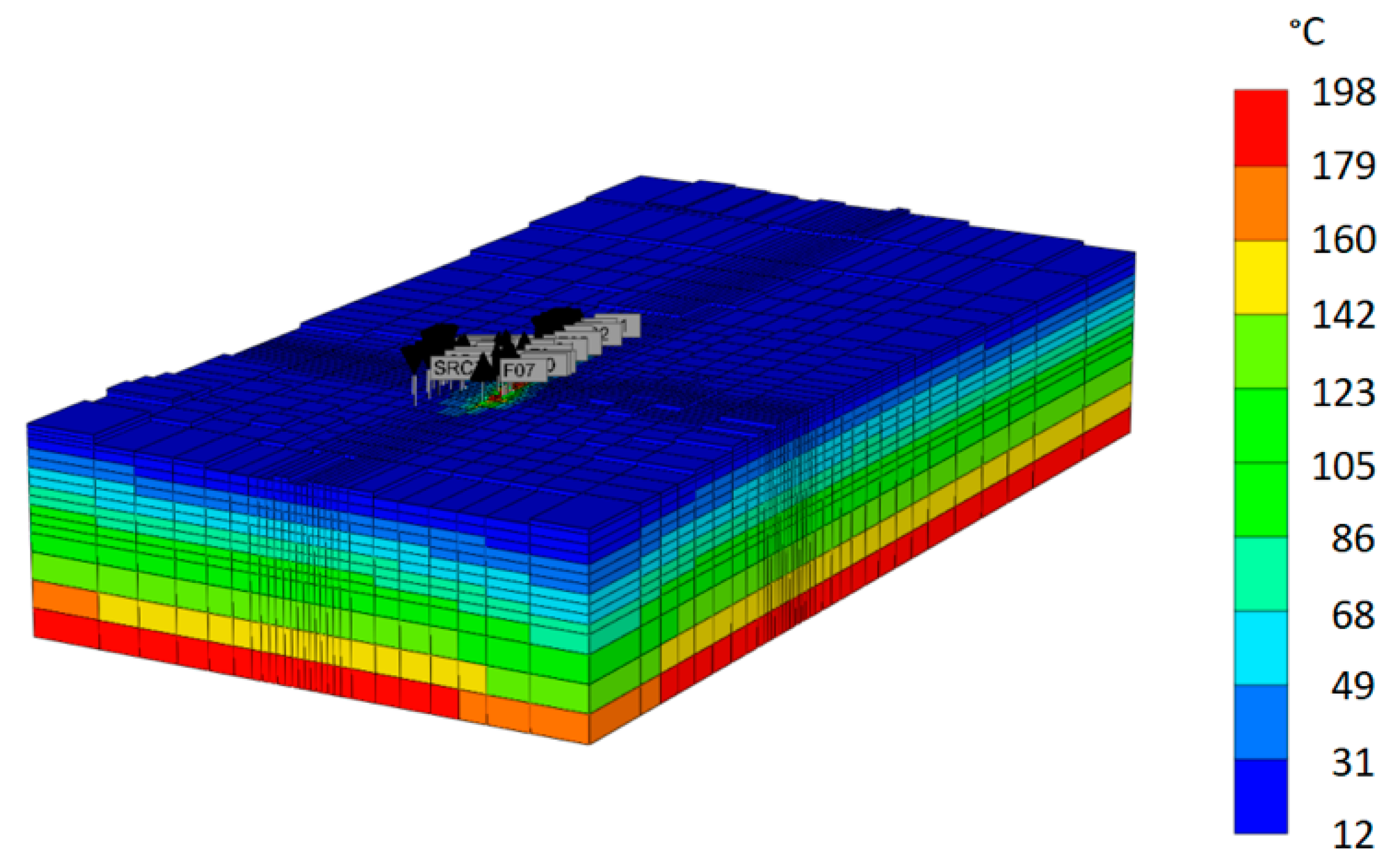
As part of this project, we upgraded Ormat’s existing BHS static geothermal reservoir model and used it to generate ML training data. The system has four injection wells and six production wells. We modified reservoir fracture flow paths, permeabilities, and porosities and ran 86 simulations using the TETRAD model to improve history matching from 1979 through 2020. The best-performing model obtained a mean absolute error (MAE) of 6 °C for production temperatures across all production wells. The model performed well in matching the tracer results from the tracer test conducted in 2019, where multiple conservative tracers were injected in four injection wells and their response was monitored in several production wells. The updated reservoir model also closely matches the early 2021 temperature survey (on average within +/− 3 °C) in a 4000-ft-deep observation well that was conducted as part of this study. We refer to this set of simulations as BHS data. A second reservoir model, in which the well locations, temperature, and permeability characteristics were arbitrarily changed, is referred to as the OSR. The OSR numerical model in CMG, color-coded by initial temperature, is shown in Figure 3. The domain dimensions are 19 km × 10 km × 3.5 km. A “hot spot” is visible near the center of the domain, where labels indicate locations of wells and boundary conditions (fumaroles at the surface and sources at the bottom).
2.3. Data Set Generation
To generate the data needed for this study, we ran 80 simulations for BHS and completed 101 simulations for OSR, all covering the 20-year period from 2020 to 2040. We chose to run 80 and 101 simulations with the idea of having two slightly different data points for the size of the training data for ML rather than studying a single size. At the same time, these numbers are large enough to represent a wide variety of scenarios, but not too large to become computationally intractable, considering the time required to run each simulation. The flow constraints were imposed upon individual wells, and the flow rates varied within the specific ranges, as shown in Table 1. The injection temperature was about 70 °C, and the injection pressure varied with the flow rate.
A representative time history for the OSR model is shown in Figure 4. The shown temperature profiles visualize one example from the simulated cases we have released as part of the OSR dataset, as detailed under the Data Availability Statement near the end of the paper.
In our work we assume no change in external conditions. Any change in the above-ground temperature and precipitation patterns is considered to have a minor impact on subsurface physics and geothermal energy production comparing to the injection well flow allocations being studied. Potential impacts of climate change, with variations in surface temperatures and precipitation, are not explicitly considered in this work.
3. Design and Implementation of Computational Pipeline
In this section, we detail our ML-based approach—from model training to inference—and discuss the nuances of all required data processing steps. We also describe the technologies that we leveraged when we turned the proposed ideas into code.
We trained our ML models to capture relationships in the reservoir data sets—more specifically, in the timeseries produced by the simulations with the aforementioned subsurface models. Thus, after the necessary training, these models are capable of reproducing those relationships and producing estimates of the quantities of interest (e.g., pressure and temperature values and then, after additional postprocessing, energy estimates), even for the scenarios that were not part of the training data sets. To be clear, these new scenarios should be similar to the ones in the training data, in the sense that the same key physical phenomena are in effect for the modeled system; otherwise, the predictions may become inaccurate. For instance, if new scenarios allow previously inactive wells to become active, the models cannot adequately predict the outcomes without a sufficient amount of representative training data. At the same time, for a fixed number of active wells, it should be possible to vary the allocation and get accurate model predictions—this is exactly the hypothesis that we are validating through this study.
It is worth highlighting the ways in which our current ML work differs from our previous efforts [23,24]. Previously, we started modeling BHS by leveraging ML techniques. Currently, we use an approach based on a fully interconnected NN with two hidden layers (of varying sizes), which are trained to predict coefficients of the curves that approximate the timeseries of interest. This approximation conveniently serves the function of data reduction, and the goal of the NN becomes more computationally tractable. Thus, multi-headed NNs (i.e., networks with multiple neurons in the output layers) can predict all required coefficients in a single pass. In contrast, our previous work was focused on the evaluation of MLP, LSTM, and CNN network architectures in the context of timeseries prediction, with numerous single-step predictions. In Appendix B, we further compare and contrast these approaches and share information about the parameters of the corresponding NNs. We further note that the timeseries prediction from our previous work was similar to the ML methods applied to oil production modeling [28].
In the current formulation, the ML models’ goal is to find an accurate and reliable mapping between 10 flow levels (for four injection wells and six production wells—these numbers are the same for BHS and OSR) and D + 1 coefficients of the curves for the polynomial approximation of degree D. If we were to consider each of these coefficients separately, we could model them individually using regression techniques (ML-based or even simpler fitting techniques). However, for modeling entire combinations of these coefficients, we choose to leverage multi-headed NN.
Learning and Inference
We perform model training on the simulation data and create multiple ML models, one for each quantity we want to predict. This includes models for temperature and pressure timeseries for each of the production wells. In Figure 5, we depict this workflow, listing all preprocessing and model handling steps.
Next, we discuss each of these steps in further detail.
- Renaming: Since TETRAD and CMG STARS produce data in the form of tables that have different column names, there is a need for input standardization. We map names like “Flow PXX (kkg/h)” onto names like “pm1” (i.e., mass flow for production #1). This mapping can be undone at the end of the pipeline to present the results in the original terms.
- Time conversion: We map individual dates in the studied timeseries, which represent the time intervals between 2020 and 2040, onto points in the [0, 1] range. Similar to the previous step, original dates can be obtained at the end by inverting this linear transformation. We use this time conversion step to make sure that the following ML process remains general enough, supporting time periods of arbitrary lengths.
- Scaling: For each input variable, we scale the values to the [0, 1] range, using global minimum and maximum values for all values of the corresponding type: temperature, pressure, or mass flow. In other words, all temperature timeseries are scaled using the same minimum and maximum values found in the arrays of historic and simulated data; the same is true for the pressure and mass flow scaling. This type-specific scaling allows us to preserve data relationships that would otherwise be lost if each timeseries was scaled irrespective of the rest of the data.
- Input consolidation: Although each flow rate can change over time in an arbitrarily complex way, we consider a simpler case: a step function according to which the historic flow rate changes to the new, studied value at the beginning of the simulated period. Obviously, a sequence of flow adjustments can be represented by a series of such steps. Using this consolidation, we create the input data set for ML training, which takes the shape of N values for N wells for which the flow can be controlled. These N values represent the individual flows for the active injection and production wells and together constitute the new flow allocation. We refer to the individual unique allocations as the studied scenarios. For C scenarios in the training data, we end up with a C * N matrix, which becomes the input for ML training (typically referred to as matrix X in ML terms).
- Polynomial approximation for output: Similar to input consolidation, we are looking for a way to represent a lengthy timeseries of interest with only a handful of numbers that represent an approximation for a given timeseries with pressure or temperature values for each well. Counting on the fact that we can decide how many such numbers are going to be involved in this approximation in each specific case, we propose obtaining these numbers from the values in the output layers of the NNs we are going to train. A polynomial approximation meets the needs of this step for the following reasons: (1) obtaining coefficients for a given timeseries’ approximation is a computationally inexpensive task (typically performed using the method of least squares); (2) reconstructing the timeseries using a set of polynomial coefficients is also straightforward and fast; and (3) based on the timeseries for temperatures and pressures obtained in the simulations we have inspected in this work, we conclude that their smooth shapes can be approximated using polynomials very accurately. Appendix A includes the figures that illustrate these shapes and characterize the errors of the curve fitting. In summary, using a polynomial of degree D will result in D + 1 coefficients, and, if used consistently across C scenarios, it will produce the C * (D + 1) matrix that will be used in training (referred to as matrix Y in ML terms). For each of the considered scenarios, a scaled approximated output value (temperature or pressure), represented by and corresponding to the (scaled) moment of time would be calculated as:where are coefficients of the approximating polynomial.
- Model training: This refers to the optimization process that minimizes the specified loss function. We use the MAE loss and rely on the code provided by TensorFlow [29], a commonly used open-source platform for ML, in driving this optimization. Model training takes place in both the cross-validation process, as explained below, and also in training of the “production” models, i.e., the ones that are ready for final evaluation and application in decision making.
- Model evaluation and selection of models with smallest prediction errors: Each of the trained models is evaluated on the data that was not used in the training using the mean absolute percentage error (MAPE). This analysis of the models’ predictive ability allows us to choose the best parameters of the models (e.g., the size of the NNs being trained) and their training (e.g., the number of iterations in the training algorithm), which is the main goal of the cross-validation process. When the values of those parameters are identified, we can proceed to train the production models.
In the inference phase, we use the trained production models, as shown in Figure 6. We select a particular flow allocation to be studied, scale the flow values to make them consistent with the training data, and then use them as input for the pressure and temperature models. The models produce predictions of the curve coefficients, which we then convert into timeseries. At the end, those predicted timeseries are comparable to the timeseries in the simulation data, i.e., they represent the same 2020–2040 period and have unscaled values. The inference is repeated for as many cases as we need to study and can be run in parallel (e.g., on several compute nodes on a supercomputer) for time efficiency.
After we obtain pressure and temperature predictions for individual wells, as described above, we can estimate reservoir-wide characteristics, such as the amounts of energy produced. Specifically, we calculate the total amount of produced energy (in units of W, later converted to MW) by summing up contributions from the active production wells. One production well’s contribution is estimated as the difference between produced enthalpy, in J/kg, and injected enthalpy, in J/kg (the latter is kept constant for all wells) multiplied by the flow rate for the well, in kg/s:
In these calculations, we assume the dead-state condition to be at 20 °C and 1 bar. In the presented equation, the enthalpy for each production well is a function of the produced temperature and pressure, and we calculate them by using the thermo-physical property tables for pure water, also known as the steam tables [30]. We integrate the calculated power estimates over time to estimate the amount of cumulative thermal energy (in MWh) produced between 2020 and 2040.
4. Studying the Open-Source Reservoir
We begin our OSR analysis with cross-validation for ML, as outlined in the previous section. As demonstrated in Appendix C, we use the k-fold cross-validation technique [31] to select the best model and training parameters for the studied data. Over 8000 “trial” models were fit using a computing allocation on Eagle [32], NREL’s supercomputer, with the goal of finding the model configurations that would allow the models to generalize, i.e., perform well on the unseen data. Although an evaluation of this kind may be computationally intractable for models of larger sizes and larger data sets, we were able to perform a grid-search-style optimization and assess 72 combinations of parameters that characterize the models and the training process for 12 quantities of interest using just a fraction of the Eagle’s allocation dedicated to this project. Thus, this cross-validation was completed after 39 h of model fitting and evaluation on one of Eagle’s compute nodes.
After cross-validation, we trained the models on the entire training set, with only the test subset (a randomly selected 10%) being held out for final model evaluation. We followed the process depicted in Figure 6 to obtain pressure and temperature curves, which we then compared with the simulation data in the test data set. In each case, we calculated the MAPE, capturing the magnitude of relative difference. The distributions of these error measures are shown in Figure 7. In the same figure, we show a visualization of one predicted curve and how it closely follows the simulation data, which, for the purposes of this evaluation, are treated as “ground truth.” To summarize, the errors in pressure predictions are in the range between 0.13% and 3.68%, with an average of 0.57%; similarly, for the errors in temperature predictions, the range is between 0.17% and 4.75%, and the average is 1.34%.
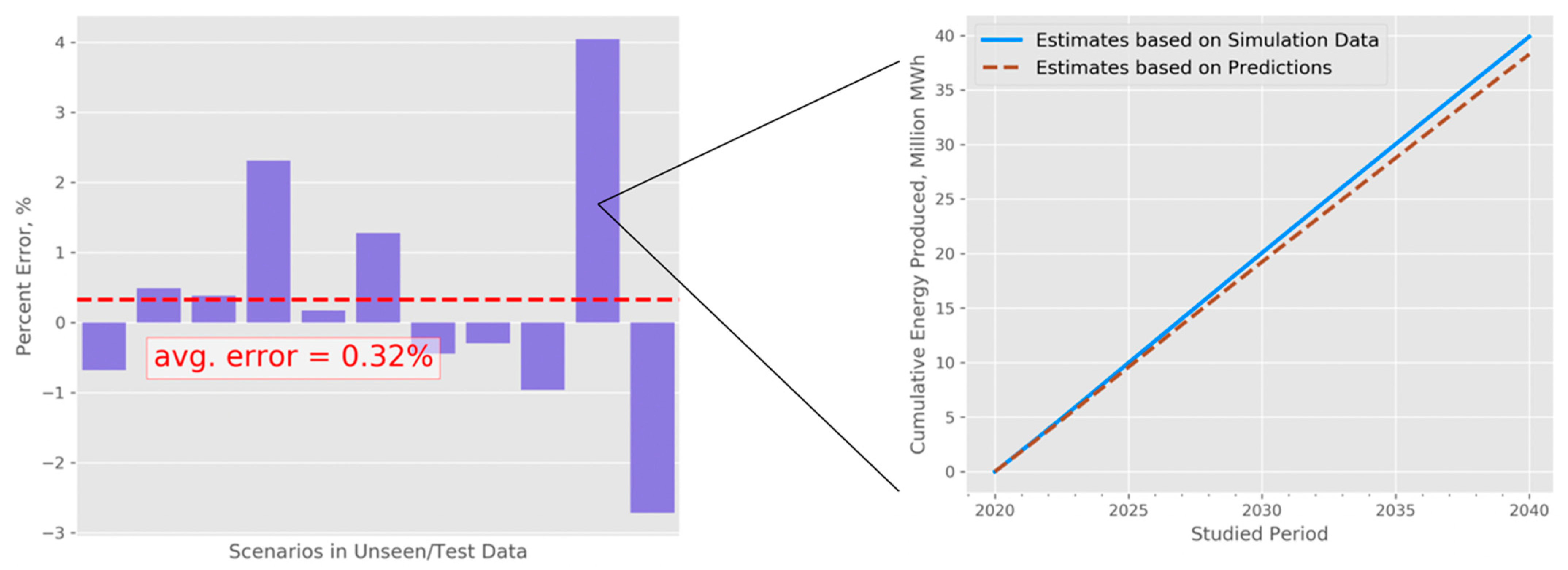
Using the selected trained models, we obtained energy estimates, as described in Section 3. We then calculated the total cumulative energy produced by the end of year 2040 using both the simulation data and our predictions, and we compared the two results. We show our results for the 11 test cases in Figure 8. In the same figure, we also visualize one specific test case and how it develops over time, in the interval from 2020–2040. These results, where the average percent error is as low as 0.32% and the worst-case error is 4.04%, indicate that the models fit the data very accurately. It is worth noting that in this analysis we averaged the real prediction errors—positive and negative (as opposed to absolute values)—obtained for the test cases, and the average of 0.32% indicates that the bias in our predications is small.
The error summaries shown in Figure 7 and Figure 8 indicate that the trained NN produced models accurately predict characteristics of OSR and generalize to the unseen data. It is also evident that the amount of used training data (i.e., 101 simulated scenarios) is sufficient for obtaining satisfying prediction accuracy.
We further characterized the robustness of the trained models by performing sensitivity analysis. The idea here is that, for good models, relatively small changes in the input should not lead to disproportionally high variability in the predicted metrics. Furthermore, by varying inputs one at a time, we can detect where the prediction sensitivity is the highest in relative terms, which would be informative to anyone who is interested in using this type of model. To proceed with such analysis, we leveraged a formulation for the “classical one-at-a-time” sensitivity index [33], defined as a partial derivative of the function R, which takes the input S, and is evaluated at a particular point in the input space :
where is the change applied to the input, and in the numerator denotes the absolute value. We adapted this formulation to our energy estimation as follows:
where is the ML-based estimate of the cumulative amount of energy produced by the end of the year 2040, F is one of the flow combinations from the training set, and is the change applied to one of the flows in the studied combination. The resulting index characterizes the cumulative amount of thermal energy and has the unit of MWh per kg/day, because MWh and kg/day are the units used for energy values and flow rates in this work, respectively. In Figure 9, we show the distributions of the sensitivity index values, , we obtained in evaluating this index on all 101 cases in the OSR data set. For all these cases, this index is between 0.12 and 0.87 MWh per kg/day, and the sensitivity is the highest (based on average ) for production well 6, production well 5, and production well 1 (P6, P5, and P1 in the figure, respectively). Among the injection wells, are more alike, although the average is slightly higher for injection well 2 (I2).
As an illustrative example, we can consider (an index value on the higher end), which was observed for P6. This particular value refers to the instance in which P6′s flow is varied by +/− 5%, and varies in response, going from to MWh, which is, in relative terms, only a 1.86% change. For a single-well change in the input, this appears to be a reasonable and modest response in a metric such as the aggregate estimate. We do not have reference numbers with which this result can be compared, and we believe more work is needed to thoroughly study sensitivity measures and, for instance, track how such measures change as the amount of training data increases. Our initial assessment of the observed values leads us to believe that there is currently no problematic variability in the model outputs. This sensitivity analysis is also an initial step toward bridging the gap of model interpretability, one of the common shortcomings in ML work, and the effort can be further expanded through the use of techniques such as individual conditional expectations and partial dependence plots [34]. Furthermore, shapely additive explanations [35] can help with interpretability and reveal more insights into relative feature importance.
5. Application to a Real-World Reservoir
Similar to our OSR analysis, we perform error analysis for the predictions obtained using the models trained on the BHS data. Through cross-validation, we confirm that the NN architecture and the chosen amount of training provide the best results among the studied configurations. Results for the production models are shown in Figure 10. Prediction errors can be summarized as follows. Predictions for pressure values show errors between 0.03% and 0.52%, with an average of 0.25%, and the temperature prediction errors are between 0.11% and 3.54%, with an average of 0.83%. For the cumulative energy estimates, we observe errors between 0.59% and 2.20%, with an average of 0.95% (we averaged positive and negative error estimates to characterize bias). We notice that these models show similar level of accuracy to the models we trained for OSR (see the results presented in the previous section). Minor differences are likely originating from the fact that one out of the 10 wells studied at BHS had zero flow (the model was developed for a ten-well reservoir, but the data from the operator suggested that one specific well was no longer considered active); thus, the BHS models focused on learning the relationships in the data for a nine-well system, as opposed to the full 10-well system represented by the OSR data. For these two reservoirs, we used the same hyperparameters (i.e., degree of approximating polynomial, sizes of NN layers, and amount of model training), but the actual training (selection of model weights) was performed for each reservoir and each well independently from the rest. There might be additional insights coming from a thorough statistical comparison of the two reservoirs’ models, yet for the purposes of this study, we find it sufficient to demonstrate that all prediction errors we have observed for two reservoirs are relatively small (under 4.75%). Moreover, we could have made BHS and OSR match exactly in terms of the numbers of simulations and active wells, but instead we chose in favor of studying two slightly different datasets and summarizing a wider range of analysis results.
We continue our model evaluation with a sensitivity analysis, in the same way we performed it for OSR. We use our ML models for BHS and the code for the cumulative thermal energy estimation, to calculate the sensitivity index, . The distributions of the observed index values for different wells (nine wells with nonzero flows) are shown in Figure 11. The largest index value, MWh per kg/day, which is smaller than the index values we estimated for OSR, indicates that a small change in the model input (5%) results in a relatively small output change, confirming the model’s high stability. Similar to the OSR results, model sensitivity to the change in the injection wells’ flows is lower than the sensitivity to the change in the production wells’ flows. Considering all our results for BHS and OSR, we conclude that the selected ML approach is indeed reliable and has potential for accurately predicting characteristics of other geothermal reservoirs given a similar amount of training simulation data. On the computing side, the results shown in Figure 11 were obtained using the trained NNs relatively quickly, but, in contrast, running all 1440 additional simulations needed for such per-quantity sensitivity summary would potentially require as much as 240 days of computing time, at 4 h per simulation.
Our final analysis step involves optimization. In this step, we selected the cases with the highest predicted cumulative energy values, . For this optimization specifically, we generated a large number () of potential flow allocations to be evaluated using the same script that we used to generate the input for the TETRAD simulations. This allowed us to study the allocations quickly, through the predictions obtained using our trained models, and choose the best-performing cases. In Figure 12, we show three distributions of energy estimates: (1) for 80 training cases, on which the models were trained (in red), (2) for G generated cases (in light blue), and (3) 5% of results from the latter (in dark blue). While we cannot release the specific estimates for BHS, we can highlight the following in relative terms:
- The 250 flow allocations selected as part of the top 5% have an average that approaches the maximum for the training set. At the same time, the maximum for the top 5% is approximately 6.5% higher than the maximum for the entire training set. This relative difference can potentially translate into a substantial energy gain, considering that the absolute values for are measured in millions of MWh. It is also worth pointing out that the maximum for the training set may refer to the flow allocation, demonstrating an additional nontrivial gain with respect to the current allocation at BHS. It is important to treat this summary as a statement about the potential optimization enabled by the proposed computational approach, rather than a commentary on the efficiency of the current reservoir operation.
- These 250 best-performing flow allocations provide enough data to further study the flows for individual wells, and, specifically, to look for noticeable differences between flow values in the training cases and in the best allocations. Such differences can indicate the directions in which the respective flows need to change in order to achieve energy gains. For BHS, we compared the current flows, the distributions of flows in the training data, and the distributions of flows in these 250 cases to arrive at well-specific recommendations. These recommendations can be used to inform operational decisions or, at minimum, can serve as the basis for additional investigation through simulations using TETRAD or CMG STARS.
Over the course of this optimization, we collected prediction runtimes, capturing how much computing time (in seconds) is needed to produce all predictions—pressures, temperatures, and energy estimates—for a given case. Our results indicate that, on average, the inference takes only 0.9 s (the runtimes were measured on a single Eagle’s compute node, with dual Intel Xeon Gold Skylake 6154 (3.0 GHz, 18-core) processor and 96 GB of RAM). This is several orders of magnitude faster than running simulations with TETRAD. 3D reservoir modeling with TETRAD or another simulator which takes hours to run, because it simulates changes in rock and fluid properties associated with thermal and hydraulic processes across the reservoir, which is a much more computationally intensive process (if done at sufficient temporal and spatial resolutions) compared to using the weights of the trained NNs for translating given inputs into outputs, even for large NNs.
6. Discussion
In our work, we have proposed and evaluated a computational approach that combines geologic reservoir modeling with ML. We show how existing methods in geothermal reservoir engineering can be leveraged to produce data for training surrogate models implemented using NNs. In this section, we share several high-level perspectives on the current work and what it can enable in future work.
We can summarize our ML work through the lens of the ML-focused recommendations shared in a recent editorial by Physical Review Fluids [36]. We found the editorial to be useful and informative, and we applied its recommendations to our work as follows:
- Physical mechanisms and their interpretation: Our ML approach is based on training a set of models to predict pressures and temperatures for individual wells. We used those model predictions in a closed-form expression to obtain reservoir-wide energy estimates, as discussed in Section 3. By obtaining multiple well-specific predictions instead of training a single model for energy produced reservoir-wide, we created a more interpretable solution where we could reason about the possible causes of high or low energy estimates; we could investigate our predictions for the wells and find the pressure or temperature timeseries that were influencing the outcomes more than the rest of the predictions.
- Reproducibility: We plan to publish all relevant data for OSR and the code we have developed to make it possible for others to reproduce our findings.
- Validation, verification, and uncertainty quantification: We believe that our error analysis, sensitivity analysis, and the energy optimization process provide enough empirical evidence about the models to consider their results trustworthy. The great similarity between the results for BHS and OSR is another piece of supporting evidence. Further validation of BHS models and predictions can take place next time Ormat changes the flow allocation (and the models will need to be retrained using the newest data), but that work is outside the scope of our current investigation.
We envision that our ML efforts will pave the way for reinforcement learning (RL) [37] in future research. RL can introduce mechanisms for further coupling of ML models and simulators. For instance, the top 5% of cases described in Section 5 can form the “second round” of TETRAD or CMG STARS simulations, which would then create even more data for model training. Then, the retrained models would help find new best-case candidates again. This iterative optimization process can be repeated as many times as we see a noticeable increase in the energy estimates. At each iteration, model validation can be performed to further inform the decisions about continuing or stopping the RL process. The training of predictive models described in this study is an important prerequisite for applying RL and potentially discovering additional energy gains.
Finally, we note that open access to high-quality data is a major prerequisite to conducting research using modern, data-centric techniques. Data availability can actually stimulate the rapid advancement of an entire field. In geothermal reservoir engineering, this is a concern of particular importance, as the availability of real-world data sets—both simulation results and real reservoir data—is relatively limited. We are not aware of any other published subsurface characterization data sets, analogous to the ones we trained the models on in our work, that we could have used. Our aim was to bridge this gap when creating OSR and running an ensemble of simulations for the reservoir. Now that the relevant OSR data is published, the research community can take advantage of it in a variety of ways. For example, other researchers can take the data and evaluate a broader set of ML predictive models, searching for further optimizations and using the results from this paper as a reference point. In a different line of research, researchers can compare the published data with the simulation data from other geothermal reservoirs, the reservoirs to which they have access, and reason about the potential of ML-based optimization for those fields.
7. Conclusions
In this study, we demonstrate how geologic reservoir modeling can be used in combination with machine learning. In fact, the latter does not replace the former in this application, but rather complements it. The combination of the two computational approaches allows us to train accurate prediction models on simulation data that capture physical subsurface phenomena. We develop this novel method with the goal of enabling optimization of the energy produced at a geothermal reservoir. We tested the method on the data for Brady Hot Springs in Nevada, USA, as well as a synthetic 10-well geothermal system with realistic characteristics. In each case, we followed the proposed process—from using simulators like TETRAD and CMG STARS to model training and evaluation—and documented the details of each computational step. Our results indicate that a high level of prediction accuracy can be achieved for these systems even with medium-sized data sets (80–101 simulations). The relative error of 4.75% was the largest error we observed among all studied predictions of pressure, temperature, and energy. For Brady Hot Springs, we showed how the trained models can be used in the optimization process, i.e., in the search for optimal flow allocations and increased energy production. Among the most significant practical benefits enabled by our work is computational efficiency: whereas a typical reservoir simulation for Brady Hot Springs completes in approximately 4 h, our trained ML models yield accurate 20-year predictions for temperatures, pressures, and the amount of produced thermal energy for the entire reservoir in only 0.9 s. This computational efficiency allows the rapid exploration of many candidate flow allocations, and, based on our findings, we expect this method to be applicable to studying other geothermal reservoirs.
Author Contributions
D.D. is the lead author who worked on data curation, formal analysis, investigation, methodology, software, validation, visualization, and all stages of writing. K.F.B. contributed to investigation, validation, visualization, and writing. D.L.S. provided valuable guidance in the areas of conceptualization, funding acquisition, and resource management, as well as helping to review and edit the manuscript. M.J.M.’s involvement includes conceptualization, funding acquisition, resource management, and writing. H.E.J. is a principal investigator on this project who coordinated activities and advised the team through conceptualization, funding acquisition, data curation, formal analysis, investigation, methodology, project administration, resource management, and writing. All authors have read and agreed to the published version of the manuscript.
Funding
We acknowledge the U.S. Department of Energy’s Office of Energy Efficiency and Renewable Energy Geothermal Technologies Office for providing funding under award number DE-FOA-0001956-1551 to the National Renewable Energy Laboratory (NREL) and the U.S. Geological Survey Geothermal Resources Investigation Project. Partial funding was also provided by the U.S. Geological Survey Mendenhall and Energy and Minerals Program. Additional material support was provided by Ormat, CMG, and Quantum Reservoir Impact LLC (QRI). This work was authored in part by the National Renewable Energy Laboratory, operated by the Alliance for Sustainable Energy, LLC, for the U.S. Department of Energy (DOE) under Contract No. DE-AC36-08GO28308. The views expressed in the article do not necessarily represent the views of the Department of Energy. The U.S. Government retains and the publisher, by accepting the article for publication, acknowledges that the U.S. Government retains a non-exclusive, paid-up, irrevocable, worldwide license to publish or reproduce the published form of this work, or allow others to do so, for U.S. Government purposes. Any use of trade, firm, or product names is for descriptive purposes only and does not imply endorsement by the U.S. Government.
Data Availability Statement
The repository with the data for Open-Source Reservoir, along with the ML code we have developed, can be found at: https://github.com/NREL/geothermal_osr (accessed on 27 January 2022).
Acknowledgments
We would like to thank John Akerley and John Murphy (Ormat Technologies Inc.) for their continued collaboration and important contributions to this study. We thank the Computer Modelling Group for donating the software licenses necessary to enable these simulations. Computational experiments were performed using Eagle, the supercomputer sponsored by the Department of Energy’s Office of Energy Efficiency and Renewable Energy and located at NREL. The authors would like to also thank Caleb Phillips and Kristi Potter of NREL, and David Castineira of QRI for useful discussions.
Conflicts of Interest
The authors declare no conflict of interest.
Abbreviations
| AI | artificial intelligence |
| BHS | Brady Hot Springs, a geothermal field in northern Nevada, USA |
| CNN | convolutional neural networks |
| Eagle | NREL’s supercomputer |
| LSTM | long short-term memory |
| MAE | mean absolute error |
| MAPE | mean absolute percentage error |
| ML | machine learning |
| MLP | multilayer perceptron |
| NN | neural network |
| OSR | open-source reservoir, a contrived geothermal reservoir that resembles BHS at a high level but has a number of sufficiently modified characteristics |
| RL | reinforcement learning |
| RMSE | root mean square error |
Appendix A
In determining what type of approximation to use for the studied data, we based our decision on the shapes of the functions being approximated, their smoothness, and complexity. As shown in Figure A1, the temperature and pressure curves are quite smooth, and they can be approximated using polynomial functions. To support this claim by the numbers, we calculate the root mean square error (RMSE) values for the individual instances of this approximation (37 scenarios 6 production wells). It appears that the errors coming from the temperature approximation tend to be smaller than the errors of pressure approximation, but, more importantly, all observed approximation errors are small, with RMSE < 0.015 for all cases.
Figure A1.
Scaled temperature (left) and pressure (right) timeseries for one of the production wells at BHS. The timeseries represent 37 CMG STARS simulations for different flow allocations.
Figure A1.
Scaled temperature (left) and pressure (right) timeseries for one of the production wells at BHS. The timeseries represent 37 CMG STARS simulations for different flow allocations.

Appendix B
In Table A1, we summarize two ML approaches: the one used in our previous work, based on point prediction, and the one used in this study, curve prediction. We report several key pros and cons for each approach. We also briefly discuss the structure of the corresponding NNs in terms of the numbers of neurons that form different layers.

Table A1.
Comparison of ML approaches for prediction of reservoir characteristics.
| Point Prediction (Used in Previous Work [23,24])  | Curve Prediction (Used in Current Study)  |
|---|---|
| Pro: Many examples in the literature, with a variety of NN architectures being used (Brownlee, 2018). | Pro: This approach is more expressive and concise, making it straightforward to go from curve parameters to timeseries. |
| Pro: Allows learning and prediction of arbitrarily complex temporal patterns. | Pro: Prediction errors for moments in the distant future are not necessarily worse than prediction errors for the near future. |
| Con: Accumulation of error is likely to occur if this single-step prediction scheme is used recursively (to obtain prediction for a whole period of time). | Con: Requires specific structure of input data. We rely on the flows being set to specific values at the beginning of the time period being studied and remaining constant throughout that period. |
| Parameters of the NN: input layer: number of neurons is set to the number of consecutive time steps used in prediction (in previous work, we used L = 12 for 12 monthly steps) plus the number of additional “channels”—other factors being considered (flows in our particular problem). hidden layer(s): arbitrary number of neurons in one or more layers. output layer: single neuron for single-step predictions. | Parameters of the NN: input layer: number of neurons is set to the number of values (flows) that define each studied scenario. hidden layer(s): arbitrary number of neurons in one or more layers. output layer: number of neurons is set to the number of coefficients that define the curves within the selected type of approximating functions; for polynomials of degree D, D+1 neurons are used. |
Appendix C
Using OSR data, we trained 8640 individual models for 12 timeseries (pressure and temperature values for six production wells). Simultaneously, we studied the effects of three parameters—the degree of the approximating polynomials, the number of neurons in the NN’s hidden layers, and the amount of model training—on the accuracy of predictions. We performed this analysis using a common approach called k-fold cross-validation (with k = 10) [31], where the training data set was repeatedly shuffled and split into k subsets, out of which k − 1 were used for model training and the remaining one was used for validation. This process is designed to prevent overfitting in the course of hyperparameter selection. In each iteration of the validation process, we obtained MAPE estimates to compare the simulation data and the model predictions.
In Figure A2, we show our cross-validation results, with the 20 best-performing model configurations depicted for one pressure and one temperature timeseries. Through this cross-validation, we learned the following:
- Curve approximation should use polynomials of degree four: They consistently produce models with lower errors than for degrees five and six on the given data.
- The best models are trained with the number of epochs set to 1000: An epoch refers to one complete pass over the data set made by an ML algorithm, and our results indicate that 1000 such passes result in better models than the lower tested values, 250 and 500, with the control for overfitting enabled by k-fold cross-validation. Epochs higher than 1000 were not considered in our study because the results we obtained for 1000 epochs with our datasets showed sufficiently high accuracy.
- With the aforementioned selections, the hidden layer sizes of the NNs should be 12 and 6: This combination consistently results in the best-performing models, as we can see in Figure A2 (there, it is the second-best configuration), as well as resulting in the best models created for all six production wells. These particular sizes of the hidden layers result in the models with 245 weights being fitted to the data, sufficiently capturing complex relationships between the model inputs and outputs.
Figure A2.
Analysis of ML models trained with k-fold cross-validation (k = 10). The figures show error summaries for pressure (left) and temperature (right) predictions for one of the production wells. Each plot shows 20 model/training configurations (out of 72 evaluated) with the lowest average MAPE estimates, depicted in ascending order.

Overall, it is worth noting that the magnitudes of the observed MAPE values, where the averages and the medians are below 2% and the rare, worst-case values are around 7%, indicate that the models with these identified parameters are highly accurate.
References
- Robins, J.C.R.; Kolker, A.; Flores-Espino, K.; Pettitt, W.; Schmidt, K.; Beckers, K.; Pauling, H.; Anderson, B. 2021 U.S. Geothermal Power Production and District Heating Market Report. 2021. Available online: https://www.nrel.gov/docs/fy21osti/78291.pdf (accessed on 1 August 2021).
- Ball, P.J. A Review of Geothermal Technologies and Their Role in Reducing Greenhouse Gas Emissions in the USA. J. Energy Resour. Technol. 2020, 143, 010903. [Google Scholar] [CrossRef]
- DOE. GeoVision: Harnessing the Heat Beneath Our Feet—Analysis Inputs and Results. Geothermal Technologies Office, US Department of Energy, 2019. Available online: https://www.osti.gov/dataexplorer/biblio/dataset/1572361 (accessed on 21 November 2021).
- Ball, P.J. Macro Energy Trends and the Future of Geothermal Within the Low-Carbon Energy Portfolio. J. Energy Resour. Technol. 2020, 143, 010904. [Google Scholar] [CrossRef]
- van der Zwaan, B.; Longa, F.D. Integrated Assessment Projections for Global Geothermal Energy Use. Geothermics 2019, 82, 203–211. [Google Scholar] [CrossRef]
- Edenhofer, O.; Pichs-Madruga, R.; Sokona, Y.; Seyboth, K.; Kadner, S.; Zwickel, T.; Eickemeier, P.; Hansen, G.; Schlomer, S.; von Stechow, C. Renewable Energy Sources and Climate Change Mitigation: Special Report of the Intergovernmental Panel on Climate Change (IPCC); Cambridge University Press: Cambridge, UK, 2011. [Google Scholar]
- Pan, S.-Y.; Gao, M.; Shah, K.J.; Zheng, J.; Pei, S.-L.; Chiang, P.-C. Establishment of Enhanced Geothermal Energy Utilization Plans: Barriers and Strategies. Renew. Energy 2019, 132, 19–32. [Google Scholar] [CrossRef]
- Soltani, M.; Kashkooli, F.M.; Souri, M.; Rafiei, B.; Jabarifar, M.; Gharali, K.; Nathwani, J.S. Environmental, Economic, and Social Impacts of Geothermal Energy Systems. Renew. Sustain. Energy Rev. 2021, 140, 110750. [Google Scholar] [CrossRef]
- Matzel, E.; Magana-Zook, S.; Mellors, R.J.; Pullimmanappallil, S.; Gasperikova, E. Looking for Permeability on Combined 3D Seismic and Magnetotelluric Datasets With Machine Learning. In Proceedings of the 46th Workshop on Geothermal Reservoir Engineering, Stanford, CA, USA, 16–18 February 2021. [Google Scholar]
- Ahmmed, B.; Lautze, N.C.; Vesselinov, V.V.; Dores, D.E.; Mudunuru, M.K. Unsupervised Machine Learning to Extract Dominant Geothermal Attributes in Hawaii Island Play Fairway Data. In Proceedings of the Geothermal Resources Council’s Annual Meeting & Expo, Reno, NV, USA, 18–21 October 2020. [Google Scholar]
- Smith, C.M.; Faulds, J.E.; Brown, S.; Coolbaugh, M.; Lindsey, C.; Treitel, S.; Ayling, B.; Fehler, M.; Gu, C.; Mlawsky, E. Characterizing Signatures of Geothermal Exploration Data with Machine Learning Techniques: An Application to the Nevada Play Fairway Analysis. In Proceedings of the 46th Workshop on Geothermal Reservoir Engineering, Stanford, CA, USA, 16–18 February 2021. [Google Scholar]
- Siler, D.L.; Pepin, J.D.; Vesselinov, V.V.; Mudunuru, M.K.; Ahmmed, B. Machine Learning To Identify Geologic Factors Associated With Production in Geothermal Fields: A Case-Study Using 3D Geologic Data, Brady Geothermal Field, Nevada. Geother. Energy 2021, 9, 1–17. [Google Scholar] [CrossRef]
- Siler, D.L.; Pepin, J.D. 3-D Geologic Controls of Hydrothermal Fluid Flow at Brady Geothermal Field, Nevada, USA. Geothermics 2021, 94, 102112. [Google Scholar] [CrossRef]
- Buster, G.; Siratovich, P.; Taverna, N.; Rossol, M.; Weers, J.; Blair, A.; Huggins, J.; Siega, C.; Mannington, W.; Urgel, A.; et al. A New Modeling Framework for Geothermal Operational Optimization with Machine Learning (GOOML). Energies 2021, 14, 6852. [Google Scholar] [CrossRef]
- U.S. Securities and Exchange Commission, Ormat Technologies, Inc. (Commission File Number: 001-32347). Available online: https://d18rn0p25nwr6d.cloudfront.net/CIK-0001296445/d7111d58-b48a-49a1-aa60-7c72223b25ba.html (accessed on 21 December 2021).
- Faulds, J.; Ramelli, A.; Coolbaugh, M.; Hinz, N.; Garside, L.; Queen, J. Preliminary Geologic Map of the Bradys Geothermal Area, Churchill County, Nevada; Open-File Report; Nevada Bureau of Mines and Geology: Reno, NV, USA, 2017. [Google Scholar]
- Wesnousky, S.G.; Barron, A.D.; Briggs, R.W.; Caskey, S.J.; Kumar, S.; Owen, L. Paleoseismic Transect Across the Northern Great Basin. J. Geophys. Res. Solid Earth 2005, 110. Available online: https://webcentral.uc.edu/eProf/media/attachment/eprofmediafile_371.pdf (accessed on 21 November 2021). [CrossRef] [Green Version]
- Faulds, J.E.; Garside, L.J.; Oppliger, G.L. Structural Analysis of the Desert Peak-Brady Geothermal Field, Northwestern Nevada: Implications for Understanding Linkages between Northeast-Trending Structures and Geothermal Reservoirs in the Humboldt Structural Zone; Transactions-Geothermal Resources Council: Davis, CA, USA, 2003. [Google Scholar]
- Faulds, J.; Moeck, I.; Drakos, P.; Zemach, E. Structural Assessment and 3D Geological Modeling of the Brady’s Geothermal Area, Churchill County (Nevada, USA): A Preliminary Report. In Proceedings of the 35th Workshop on Geothermal Reservoir Engineering, Stanford, CA, USA, 1–3 February 2010; Stanford University: Stanford, CA, USA, 2010. [Google Scholar]
- Jolie, E.; Moeck, I.; Faulds, J.E. Quantitative Structural—Geological Exploration of Fault-Controlled Geothermal Systems—A Case Study From the Basin-And-Range Province, Nevada (USA). Geometrics 2015, 54, 54–67. [Google Scholar] [CrossRef] [Green Version]
- Siler, D.L.; Hinz, N.H.; Faulds, J.E. Stress Concentrations at Structural Discontinuities in Active Fault Zones in the Western United States: Implications for Permeability and Fluid Flow in Geothermal Fields. Bulletin 2018, 130, 1273–1288. [Google Scholar] [CrossRef]
- Siler, D.L.; Faulds, J.E.; Hinz, N.H.; Queen, J.H. Three-Dimensional Geologic Map of the Brady Geothermal Area, Nevada. 2021. Available online: https://pubs.er.usgs.gov/publication/sim3469 (accessed on 2 December 2021).
- Beckers, K.F.; Duplyakin, D.; Martin, M.J.; Johnston, H.E.; Siler, D.L. Subsurface Characterization and Machine Learning Predictions at Brady Hot Springs. In Proceedings of the 46th Workshop on Geothermal Reservoir Engineering, Stanford, CA, USA, 15–17 February 2021. [Google Scholar]
- Duplyakin, D.; Siler, D.L.; Johnston, H.; Beckers, K.; Martin, M. Using Machine Learning To Predict Future Temperature Outputs in Geothermal Systems. In GRC 2020 Virtual Annual Meeting & Expo; National Renewable Energy Lab: Reno, NV, USA, 2020. [Google Scholar]
- Brownlee, J. Deep Learning for Time Series Forecasting: Predict the Future with MLPs, CNNs and LSTMs in Python; Machine Learning Mastery: San Juan, PR, USA, 2018. [Google Scholar]
- Shook, G.M.; Faulder, D.D. Validation of a Geothermal Simulator; DOEEEGTP (USDOE Office of Energy Efficiency and Renewable Energy Geothermal Tech Pgm): Idaho Falls, ID, USA, 1991. [Google Scholar]
- CMG LTD. STARS Thermal & Advanced Processes Simulator. 2021. Available online: https://www.cmgl.ca/stars. (accessed on 21 November 2021).
- Nwachukwu, C. Machine Learning Solutions for Reservoir Characterization, Management, and Optimization. Ph.D. Thesis, University of Texas at Austin, Austin, TX, USA, 2018. Available online: https://repositories.lib.utexas.edu/handle/2152/74252. (accessed on 22 April 2020).
- Abadi, M.; Agarwal, A.; Barham, P.; Brevdo, E.; Chen, Z.; Citro, C.; Corrado, G.S.; Davis, A.; Dean, J.; Devin, M.; et al. TensorFlow: Large-Scale Machine Learning on Heterogeneous Systems. arXiv 2015, arXiv:1603.04467. Available online: https://www.tensorflow.org/2015 (accessed on 27 January 2022).
- Wagner, W.; Kruse, A. Properties of Water and Steam: The Industrial Standard IAPWS-IF97 for the Thermodynamic Properties and Supplementary Equations for Other Properties: Tables Based on These Equations; Springer: Berlin/Heidelberg, Germany, 1998. [Google Scholar]
- scikit-learn.org, 3.1. Cross-Validation: Evaluating Estimator Performance. 2021. Available online: https://scikit-learn.org/stable/modules/cross_validation.html (accessed on 22 November 2021).
- NREL, Eagle Computing System. 2021. Available online: https://www.nrel.gov/hpc/eagle-system.html (accessed on 22 November 2011).
- Tunkiel, A.T.; Sui, D.; Wiktorski, T. Data-Driven Sensitivity Analysis of Complex Machine Learning Models: A Case Study of Directional Drilling. J. Petrol. Sci. Eng. 2020, 195, 107630. [Google Scholar] [CrossRef]
- Molnar, C.; Konig, G.; Herbinger, J.; Freiesleben, T.; Dandl, S.; Scholbeck, C.A.; Casalicchio, G.; Grosse-Wentrup, M.; Bischl, B. General Pitfalls of Model-Agnostic Interpretation Methods for Machine Learning Models. arXiv 2020, arXiv:2007.04131. [Google Scholar]
- Lundberg, S.; Lee, S. A Unified Approach to Interpreting Model Predictions. 2017. Available online: https://arxiv.org/abs/1705.07874 (accessed on 5 January 2022).
- American Physical Society. Machine Learning and Physical Review Fluids: An Editorial Perspective. 2021. Available online: https://journals.aps.org/prfluids/edannounce/10.1103/PhysRevFluids.6.070001 (accessed on 4 December 2021).
- Arulkumaran, K.; Deisenroth, M.P.; Brundage, M.; Bharath, A.A. Deep Reinforcement Learning: A Brief Survey. IEEE 2017, 34, 26–38. [Google Scholar] [CrossRef] [Green Version]
Figure 1.
The process that combines reservoir simulations and machine learning.

Figure 2.
Inputs and outputs for high-fidelity reservoir models.

Figure 3.
CMG reservoir domain of OSR. The colors represent initial temperatures (in °C). Gray labels above the field point at the existing wells. The shown domain is 19 km × 10 km × 3.5 km.
Figure 3.
CMG reservoir domain of OSR. The colors represent initial temperatures (in °C). Gray labels above the field point at the existing wells. The shown domain is 19 km × 10 km × 3.5 km.

Figure 4.
Production temperature profiles for the six OSR production wells, P1 through P6, simulated for 2020–2040 (simulated years are shown along the x-axes). Simulations were conducted using CMG STARS.
Figure 4.
Production temperature profiles for the six OSR production wells, P1 through P6, simulated for 2020–2040 (simulated years are shown along the x-axes). Simulations were conducted using CMG STARS.

Figure 5.
Computational tasks involved in creation of ML models.

Figure 6.
The inference process and creation of timeseries predictions. “Q” could be a quantity such as temperature or pressure for one of the production wells. Specific numbers are shown in the diagram for illustrative purposes only.
Figure 6.
The inference process and creation of timeseries predictions. “Q” could be a quantity such as temperature or pressure for one of the production wells. Specific numbers are shown in the diagram for illustrative purposes only.

Figure 7.
(left) Summary of the models trained for OSR and evaluated on the unseen data (11 test cases that were set aside before model training) and (right) one illustrative example of the curve predicted for a selected test case.
Figure 7.
(left) Summary of the models trained for OSR and evaluated on the unseen data (11 test cases that were set aside before model training) and (right) one illustrative example of the curve predicted for a selected test case.

Figure 8.
(left) Relative errors in predictions for total cumulative energy (for the year 2040) and (right) one illustrative example (observed case with the largest relative error) of cumulative thermal energy produced as a function of time.
Figure 8.
(left) Relative errors in predictions for total cumulative energy (for the year 2040) and (right) one illustrative example (observed case with the largest relative error) of cumulative thermal energy produced as a function of time.

Figure 9.
Sensitivity index distributions for OSR. I1–I4 refer to the injection wells, and P1–P6 refer to the production wells. In the histograms, y-axis values characterize the number of occurrences of the corresponding x-axis values ().
Figure 9.
Sensitivity index distributions for OSR. I1–I4 refer to the injection wells, and P1–P6 refer to the production wells. In the histograms, y-axis values characterize the number of occurrences of the corresponding x-axis values ().

Figure 10.
Error analysis for BHS predictions. (left) MAPE for pressure and temperature predictions. (right) Percent errors are shown for . All results represent predictions for the subset of the data not used in the training.
Figure 10.
Error analysis for BHS predictions. (left) MAPE for pressure and temperature predictions. (right) Percent errors are shown for . All results represent predictions for the subset of the data not used in the training.

Figure 11.
Sensitivity index distributions for BHS. For anonymity, we refer to the injection wells as I1–I4 and the production wells as P1–P6. P2 has zero flow in all simulations and was skipped in the sensitivity analysis. In the histograms, y-axis values characterize the number of occurrences of the corresponding x-axis values ().

Figure 12.
Histogram of cumulative energy estimates, . The values on the x-axis are omitted to avoid releasing sensitive information.
Figure 12.
Histogram of cumulative energy estimates, . The values on the x-axis are omitted to avoid releasing sensitive information.

Table 1.
Ranges of the well flows used in OSR simulations.
| Well | Type | Simulated Flow Rate (kg/day) | |
|---|---|---|---|
| Min | Max | ||
| I1 | Injection | 3,409,880 | 10,229,650 |
| I2 | Injection | 5,056,776 | 15,170,330 |
| I3 | Injection | 10,982,070 | 32,946,200 |
| I4 | Injection | 5,389,298 | 16,167,890 |
| P1 | Production | 7,522,530 | 22,567,590 |
| P2 | Production | 3,641,546 | 10,924,640 |
| P3 | Production | 3,926,900 | 11,780,710 |
| P4 | Production | 3,906,016 | 11,718,050 |
| P5 | Production | 7,680,623 | 23,041,870 |
| P6 | Production | 3,555,400 | 10,666,210 |
Publisher’s Note: MDPI stays neutral with regard to jurisdictional claims in published maps and institutional affiliations. |
© 2022 by the authors. Licensee MDPI, Basel, Switzerland. This article is an open access article distributed under the terms and conditions of the Creative Commons Attribution (CC BY) license (https://creativecommons.org/licenses/by/4.0/).
Share and Cite
MDPI and ACS Style
Duplyakin, D.; Beckers, K.F.; Siler, D.L.; Martin, M.J.; Johnston, H.E. Modeling Subsurface Performance of a Geothermal Reservoir Using Machine Learning. Energies 2022, 15, 967. https://0-doi-org.brum.beds.ac.uk/10.3390/en15030967
AMA Style
Duplyakin D, Beckers KF, Siler DL, Martin MJ, Johnston HE. Modeling Subsurface Performance of a Geothermal Reservoir Using Machine Learning. Energies. 2022; 15(3):967. https://0-doi-org.brum.beds.ac.uk/10.3390/en15030967
Chicago/Turabian StyleDuplyakin, Dmitry, Koenraad F. Beckers, Drew L. Siler, Michael J. Martin, and Henry E. Johnston. 2022. "Modeling Subsurface Performance of a Geothermal Reservoir Using Machine Learning" Energies 15, no. 3: 967. https://0-doi-org.brum.beds.ac.uk/10.3390/en15030967
Note that from the first issue of 2016, this journal uses article numbers instead of page numbers. See further details here.