
Fault Diagnosis Technology for Ship Electrical Power System


1
School of Electronic Information, Jiangsu University of Science and Technology, Zhenjiang 212003, China
2
Electrical Design Department, Zhenjiang Hongye Science & Technology Co., Ltd., Zhenjiang 212000, China
3
Mechanical Design Department, Zhenjiang Hongye Science & Technology Co., Ltd., Zhenjiang 212000, China
*
Author to whom correspondence should be addressed.
Energies 2022, 15(4), 1287; https://0-doi-org.brum.beds.ac.uk/10.3390/en15041287
Submission received: 26 December 2021
/
Revised: 3 February 2022
/
Accepted: 4 February 2022
/
Published: 10 February 2022
(This article belongs to the Special Issue Management of Energy and Manufacturing System)
Abstract
:This paper proposes a fault diagnosis method for ship electrical power systems on the basis of an improved convolutional neural network (CNN) to support normal ship operation. First, according to the mathematical model of the ship electrical power system, the simulation model of the ship electrical power system is built using the MATLAB/Simulink simulation software platform in order to understand the normal working state and fault state of the generator and load in the power system. Then, the model is simulated to generate the fault response curve, and the picture dataset of the network model is obtained. Second, a CNN fault diagnosis model is designed using TensorFlow, an open-source tool for deep learning. Finally, network model training is performed, and the optimal diagnosis results of the ship electrical power system are obtained to realize structural parameter optimization and diagnosis. The diagnosis results show that the established simulation model and improved CNN can provide support for fault diagnosis of the ship electrical power system, improve the operation stability and safety of the ship electrical power system, and ensure safety of the crew.
1. Introduction
With the continuous development of modern technology, ship electrical power systems that can realize overall coordination of the energy of the entire ship are expected to constitute the development trend of ships in the future [1,2]. Ship electrical power systems are significantly different from land power systems [3]. In particular, they are strongly independent. Because ship electrical power systems have a smaller capacity than onshore power systems, bus voltage fluctuation may occur under the application or removal of a large load, which can easily cause serious faults. Any equipment fault in the system can affect the entire power grid. If potential safety hazards occur during operation, they will threaten the safety of the entire ship. Ship electrical power systems are regarded as the core of the entire ship. They are independent and have high requirements in terms of safe operation and fault diagnosis. They need faster and more accurate fault diagnosis than land power systems in case of system faults [4]. Therefore, fault diagnosis technologies are necessary to study ship electrical power systems [5].
Fault diagnosis of a ship electrical power system entails modeling and simulation of the system. Early modeling methods mainly involved physical modeling, i.e., a physical model was established using the similarity principle. At present, the mathematical modeling method is mainly used. This method can abstract the internal characteristics of the system into mathematical formulas, deduce the internal characteristics of the actual system, and diagnose faults through changes in the relationship between the independent variables and the dependent variables of the mathematical formulas. Research on modeling and simulation of ship electrical power systems is based on the power system model and involves a series of studies on how to maintain system stability. The ship electrical power system model is integrated with the modules of each basic unit. First, a mathematical model is established for each basic unit of the power system according to the structure and basic principles of the ship electrical power system. Then, a simulation model is built to form a complete ship electrical power system model [6]. The research process should include modeling and simulation technologies, automatic control, and other theoretical methods. In particular, the generator and its excitation are related to the voltage stability of the power system. The linear single variable control method, which was first used in excitation control, has been subsequently modified into the nonlinear multivariable control method. The development of the excitation control method has undergone several stages [7], from the earliest classical proportional integral and differential (PID) control method to the multivariable control method based on modern theory. At present, it is applied as an intelligent control method. In [8], the authors proposed a T-S fuzzy-weighting-based excitation switching control method for a tidal generator set, which can overcome the dynamic and static performance defects in the excitation control of the tidal generator set and improve its performance. In [9], feedback control was adopted for the field currents of the two-phase brushless exciter, and speed reference control was adopted for the excitation frequency and phase sequence; this method achieves a constant field current for the main generator. In [10], the authors presented a nonlinear coordinated excitation and static VAR compensator (SVC) control for regulating the output voltage and improving the transient stability of a synchronous generator infinite bus (SGIB) power system. In terms of the mathematical development of fault diagnosis methods for ship electrical power systems, the author in [11] developed a higher-order mathematical model of the generator to describe the generator state in greater detail. In [12], the authors proposed three different mathematical models for the mathematical modeling of a synchronous generator, used the models under different working conditions, and conducted a detailed comparative analysis of the models to improve the simulation accuracy.
In general, fault diagnosis methods are currently categorized into three main types [13], namely fault diagnosis based on analytical modeling, fault diagnosis based on signal processing, and fault diagnosis based on artificial intelligence. Analytical modeling includes state and parameter estimation as well as consistency testing. It has the characteristics of real-time diagnosis and the essence of deep human systems. However, it also has some defects, such as a large modeling error and significant noise interference. Signal processing includes spectrum analysis and wavelet transformation. It has the advantages of simple application and good real-time performance. However, it cannot deal with potential faults. Artificial intelligence [14] includes neural networks, fuzzy theory, genetic algorithms, rough sets, artificial immune systems and fuzzy cluster analysis algorithms, fault trees, and support vector machines, which have strong learning and reasoning abilities. To overcome key faults such as a broken rotor bar or electrical phase fault, a fault diagnosis method for the electric drive of an electric ship has been proposed [15]; however, the number of fault diagnosis objects is insufficient. In [4], the proposed load monitoring and fault detection method outlines a data-clustering-based approach to extract unique feature vectors from short-time Fourier transform analysis for any pulsed load; however, this method is not suitable for any general load curve integrated solution. In [16], the location and severity of a stator winding fault of a permanent magnet synchronous motor were modeled and detected, and a mathematical model that can describe both the health state and the fault state was established; however, the mathematical model is not suitable for other ship electrical power system equipment. In [17], a remote system was introduced for online condition monitoring and fault diagnosis of a gas turbine on an offshore oil well drilling platform on the basis of a kernelized information entropy model. In [18], a multi-class multi-core correlation vector machine fault diagnosis method based on manifold learning and swarm intelligence optimization was proposed to improve the predictive maintenance activities of diesel engines.
This paper proposes an improved network fault diagnosis model based on a convolutional neural network (CNN). This method can directly input the original image without feature decomposition and extraction. It has significant advantages, such as simple ap-plication, high operation speed, automatic parameter updates, and stable, convergent, and accurate results. These advantages enable the method to overcome existing drawbacks in the fault diagnosis of ship electrical power systems. First, based on the MATLAB/Simulink (The MathWorks Inc., Natick, MA, USA) simulation software platform, the ship electrical power system simulation model is established to understand the normal working state and fault state of the generator and load. Then, the fault response curve is generated and the picture dataset of the network model is obtained. Second, the CNN fault diagnosis model is designed using TensorFlow, an open source tool for deep learning. Finally, network model training is performed, and optimal diagnosis results are obtained to realize structural parameter optimization and diagnosis.
2. Ship Electrical Power System
2.1. Model of Excitation Control System
At present, most ships use AC electric propulsion systems. Because the electrical equipment of the ship mainly comprises inductive loads, the load current will cause demagnetization of the synchronous generator, and the load change will alter the power grid voltage of the ship [19]. To ensure stable operation of the power system, the excitation system will adjust the excitation current supplied to the generator according to the load change, make the generator terminal voltage return to the given value, and realize stability of the generator terminal voltage.
Currently, the most common excitation mode of generators in ship electrical power systems is phase compound excitation of brushless excitation systems. The combination of brushless excitation and automatic voltage regulation (AVR) can effectively enhance the forced excitation capacity and reaction speed of the excitation system. The principle of the excitation system is that the rotating exciter rotates at the same speed as the magnetic field of the main generator, and the auxiliary exciter rotates with the rotating exciter.
AVR plays an important role in phase compound excitation systems [20]. The power supply unit in AVR converts the output voltage of the generator into the voltage required by the system through voltage transformation, rectification and other links, and then transmits the results to the PID control unit and phase control unit. The synchronous control unit controls and adjusts the phase change of the excitation current output through the exciter to maintain the same change as the phase change of the applied thyristor excitation voltage. The voltage difference detection unit monitors the error signal between the reference voltage and the actual voltage in the system. The PID control unit amplifies the voltage error signal. The phase control unit mainly amplifies the signal. The main thyristor rectifier unit mainly rectifies the armature current of the static exciter.
Based on the above-mentioned principles and by referring to the excitation system model recommended by IEEE [21], the mathematical model of the excitation system can be obtained as follows:
- (1)
- Mathematical model of phase compound excitation device is represented by d and q components as follows:
- (2)
- Mathematical model of voltage difference
The model of voltage difference is an adder model, which compares the effective voltage signal input of other elements and obtains a voltage difference signal as a control signal. The difference between the output terminal voltage and the set voltage satisfies Equation (3):
where is phase compound excitation voltage signal, is the time constant of the filter, is the reference voltage of the automatic voltage regulating device, is the voltage difference between the output terminal voltage and the set voltage, is the initial excitation voltage, is the effective gain of the exciter, is the grounding voltage of power system (0), and is the feedback output voltage.
- (3)
- Amplifier mathematical modelThe mathematical equation that the amplifier satisfies is:
- (4)
- Mathematical model of lead–lag compensatorThe mathematical equation that the lead–lag compensator satisfies is:
- (5)
- Mathematical model of proportional saturation elementThe mathematical equation of proportional saturation element is:
- (6)
- Simplified exciter mathematical modelExciter is usually represented by one-order inertia element, as shown in Equation (7):
- (7)
- The mathematical equation that the feedback stabilization element satisfies is:
2.2. Simulation Model of Diesel-Driven Synchronous Generator and Its Excitation System
According to the above-mentioned mathematical model, the simulation model of the excitation control system [22] is established using simulation software as follows:
As shown in Figure 1, the main regulator and lead–lag compensator, as the main controller and damping feedback link, constitute a closed-loop PID control loop. Input vref is the set value of the synchronous generator terminal voltage, vd and vq are the voltage values on the d-axis and q-axis of the generator, respectively, and vstab is the synchronous generator ground zero voltage. The output terminal Vf of the excitation control system is the excitation voltage. In addition to the corresponding parameters of each link shown in Figure 1, the initial excitation voltage Vf0 is set to 1, and the upper and lower limits of the proportional saturation link for the limiting amplitude are 5 and 0, respectively.
The power unit of the power system of the ship adopts diesel fuel combination for combined power. The main power unit is the synchronous generator driven by diesel, while the auxiliary power unit is the asynchronous generator driven by a gas turbine. The synchronous generator is the synchronous generator simulation model in the MATLAB/Simulink/SimPowerSystems module library, and its parameters are listed in Table 1. To ensure stability and correctness of the simulation graphics, it is also necessary to use the built-in function of the powergui module in Simulink in order to initialize the generator.
2.3. Simulation Model of Gas-Turbine-Driven Asynchronous Generator
The auxiliary power unit gas turbine has a complex structure. To better simulate the operation, the turbine part of the of gas turbine is used to replace the entire gas turbine [23], as shown in Figure 2.
The turbine uses a two-dimensional look-up table to calculate the turbine torque output (TM) as a function of the gas speed (w speed) and turbine speed (w turbo) of the gas turbine.
The asynchronous generator is the asynchronous generator simulation model in the MATLAB/Simulink/SimPowerSystems module library. Its parameters are listed in Table 2.
2.4. Discrete Frequency Regulator
Figure 3 shows the simulation model of the discrete frequency regulator [24]. The frequency is controlled by the discrete frequency regulator module. The controller uses a standard three-phase phase locked loop (PLL) system to measure the system frequency. The measured frequency is compared with the reference frequency (60 Hz) to obtain the frequency error. The error is then integrated to obtain the phase error. Further, the proportional differential (PD) controller uses the phase error to generate an output signal representing the required secondary load power. The signal is converted into an 8 bit digital signal to control the switching of eight three-phase secondary loads. To minimize voltage interference, switching occurs when the voltage crosses zero.
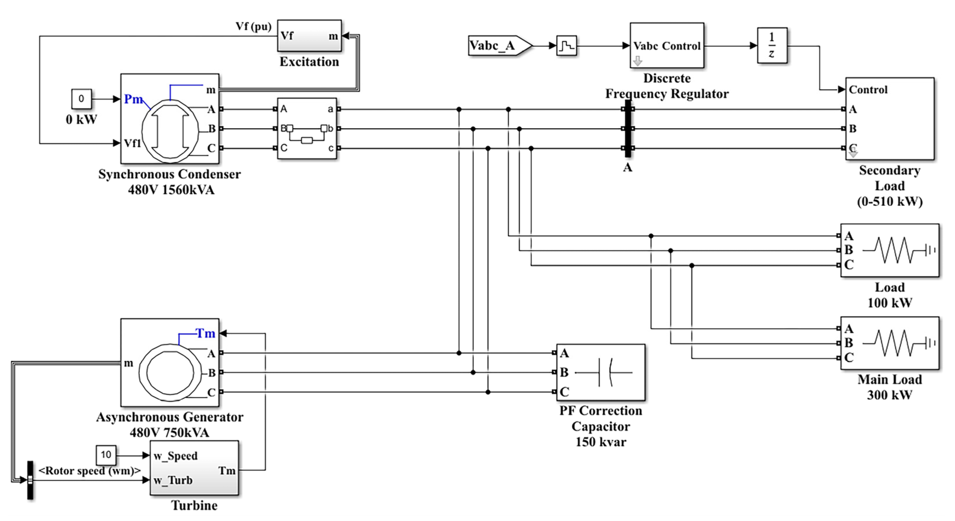
2.5. Ship Electrical Power System Simulation Model
The ship electrical power system model consists of the diesel-driven main generator set module, gas-turbine-driven auxiliary generator set module, and power load. The main load is 300 kW [25]. The secondary load block consists of eight groups of three-phase resistors connected in series with the GTO thyristor switch. The nominal power of each unit follows a binary series; thus, the load can be varied from 0 to 510 kW in steps of 2 kW. The GTO is simulated by an ideal switch. In summary, the simulation model of the ship electrical power system can be obtained as shown in Figure 4. A, B and C are phase lines.
2.6. Typical Fault Simulation of Ship Electrical Power System
Ship electrical power systems are different from land power systems. In particular, ship electrical power systems are strongly independent. A component fault in the ship power grid may affect the entire power grid. Short-circuit faults and open-phase faults are typical faults that pose serious threats. Such faults affect not only individual equipment but also the power grid of the entire ship. In severe cases, they may lead to paralysis of the ship power grid. As shown in Table 3 short-circuit faults include single-phase short-circuit grounding, two-phase short circuit, two-phase short-circuit grounding, and three-phase short circuit, while open-phase faults include single-phase disconnection and two-phase disconnection. It is necessary to simulate and diagnose the state of short-circuit and open-phase faults as typical faults in ship electrical power systems.
There are many reasons for short-circuit faults [26], such as line aging, component damage, corrosion and ring breaking in the working environment of the ship, and component insulation. Short-circuit faults pose serious threats, as they may burn important equipment, interfere with nearby communication, endanger life, and even lead to power grid collapse and loss of power supply for the entire ship. For ship electrical power systems, any type of short-circuit fault can not only threaten the safety of the entire ship power grid but also produce various problems such as electromagnetic interference. Open-phase faults, similar to short-circuit failure, will also has devastating effects.
Based on the simulation model of the ship electrical power system, the “three-phase fault” fault module of Simulink is added at the synchronous generator, asynchronous generator, main load, and secondary load ends to set the time of fault occurrence and simulate typical single-phase short-circuit grounding faults, two-phase short-circuit faults, two-phase short-circuit grounding faults, and three-phase short-circuit faults [27]. A “three-phase breaker” is used to set the occurrence time of open-phase faults and simulate typical single-phase disconnection and two-phase disconnection.
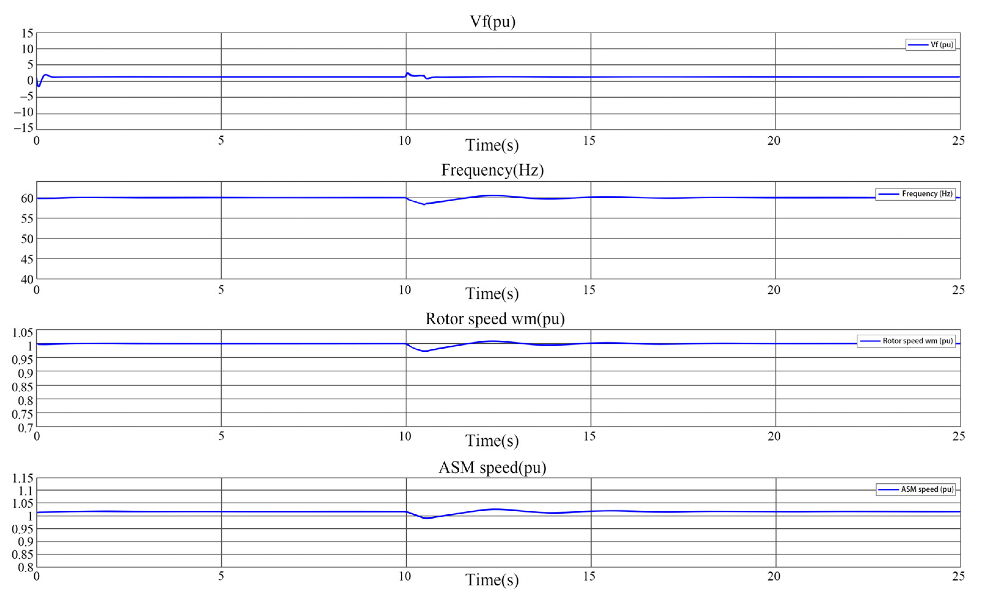
This section describes single-phase short-circuit grounding faults at the synchronous generator end. During normal operation, the three phases are symmetrical; hence, regardless of which phase of ABC is grounded, the changes in the short-circuit faults are basically the same. The single-phase short-circuit grounding fault simulation is performed by taking phase a as an example. The fault module is set to phase a grounding in 10 s, the fault module is cut off in 10.5 s, and the total simulation time is 25 s. Before 10 s, the entire power system was in stable operation. At 10 s, the fault module caused phase a short-circuit grounding fault, and the fault was removed after 0.5 s. The simulation results are shown as response curves in Figure 5. When different faults occur in different equipment of the power system of the ship, the amplitudes of the four output response curves in the fault time period are different from the normal waveform, and the differences are significant. Therefore, this is used as the basis for fault diagnosis.
The abscissa represents time, and its unit is second (s). Vf (pu) is the unit value of the excitation voltage, Frequency (Hz) is the system frequency, rotor speed wm (pu) is the unit value of the synchronous generator speed, and ASM speed (pu) is the unit value of the asynchronous generator speed.
It can be seen that in the initial stage of the ship electrical power system, the system tends to be in stable operation after starting, and the speed, excitation voltage and frequency of the two generators have not changed, and the entire power system has not fluctuated significantly. At 10 s, the fault module “Three-Phase Fault” causes the single-phase short-circuit grounding fault of Phase A, and the short-circuit current in phase A, generator speed, excitation voltage and frequency fluctuate greatly. The single-phase short-circuit grounding fault affects the stability of the power system and makes the ship unable to run normally. At 10.5 s, the fault module “Three-Phase Fault” is removed, and the single-phase short-circuit grounding fault disappears. After adjustment by the excitation control system, the ship electrical power system returns to normal; the speed, excitation voltage, and frequency of the two generators return to stability. Similarly, the simulation results of two-phase short-circuit, two-phase short-circuit grounding, three-phase short circuit, single-phase disconnection, and two-phase disconnection at the synchronous generator end are shown in Figure 6. The faults at the asynchronous generator, main load, and secondary load ends will not be repeated.
3. Construction of Improved CNN
3.1. CNN
CNN has emerged as a research hotspot in many scientific fields, especially pattern classification [28]. CNN is composed of a series of layers, as well as data flows between the layers. The basic structure is as follows: input layer, convolution layer, activation function, pooling layer, and fully connected layer, i.e., INPUT-CONV-RELU -POOL-FC.
The convolution layer is a feature extraction layer. The input of each neuron is connected to the local receptive field of the previous layer and extracts local features. The convolution layer mainly convolutes the image according to the convolution kernel and reduces noise [29]. It also involves the principle of “weight sharing”. The calculation formula of the convolution layer is as follows:
where denotes the number of layers, represents the feature graph set of the previous layer associated with the the feature graph of the current layer, is the th characteristic diagram output by the th layer, is the th characteristic diagram of the output of the th layer, is the convolution kernel between the th characteristic graph of the th layer and the th characteristic graph of the previous layer, and is the offset of the th characteristic graph of the th layer.
The activation function is used to add nonlinear factors, because the convolution method is used to deal with linear operations, i.e., assign weights to each pixel. The expression of the linear model is not sufficient; hence, an activation function is required. Common activation functions include the sigmoid function, tanh function, ReLU function, and leaky ReLU function.
The pooling layer is a feature mapping layer. After adding bias, a new feature map is obtained in the pooling layer through a nonlinear function [30]. The functions of pooling are as follows: (i) reducing the size of the characteristic diagram and simplifying the computational complexity of the network; (ii) feature compression to extract the main features. The operation formula of the pooling layer is as follows:
where represents the pooled down-sampling function, is the ratio column offset, and is the additive bias.
The fully connected layer is used to connect all the features and send the output value to a classifier (such as a softmax classifier) for classification.
Finally, the test accuracy and error loss function value of the model are output. The structure and parameters of CNN are shown in Figure 7.
3.2. Improved CNN
The traditional model has a complex structure, massive parameters, and low running speed. Moreover, the convergence speed of the classification results is affected by the method of initializing the parameters and the updating of the network weights, and there are oscillation problems in the accuracy and loss rate curves. In summary, this study makes the following improvements and proposes a CNN model with better performance, which can avoid the above-mentioned issues.
- (1)
- All local response normalization (LRN) layers are removed and the initial value program is changed. It is proven by practice that the normalization operation of batch normalization (BN) is used after simple parameter initialization. The use of BN is conducive to the convergence of the samples and the stability of the network.
- (2)
- The number of nodes in the fully connected layer is adjusted; based on the reduction and updating of parameters and weights, the running speed is improved and the calculation time is shortened.
- (3)
- Nesterov-accelerated adaptive moment estimation (NAdam) is used to update the weights of the neural networks iteratively on the basis of the training data, and the weights can be updated iteratively according to the output results.
- (4)
- Kaiming initialization is used to initialize the normal_initializer. After testing, the results will be improved.
3.3. Flow of CNN Algorithm
The algorithm flow of the proposed CNN fault diagnosis model is shown in Figure 8. It is mainly divided into four stages:
- (1)
- Sample image preprocessing: First, the sample dataset is constructed. Second, the size and color of the image are processed to facilitate network learning.
- (2)
- Design network fault diagnosis model: Network programs are written and built in the Python (Python Software Foundation, Delaware, USA) compilation environment and TensorFlow (Google Brain, San Francisco, USA) learning framework.
- (3)
- Training optimization network model: The weight and threshold are adjusted repeatedly according to the back propagation (BP) algorithm in order to minimize the error signal.
- (4)
- The optimized model is tested on the sample image dataset to output the diagnosis results.
3.4. Data Preprocessing
This study employs MATLAB/Simulink to build the ship electrical power system and takes the waveform of fault response curve as the input of the network fault model. Data preprocessing is divided into the following parts: data acquisition, image culling and data normalization.
- (1)
- Data acquisition: In the simulation model, different faults in the “three-phase fault” fault module are set for different generators and loads to output the fault response curve. The file type is the JPG-format picture set recognized by CNN.
- (2)
- Image culling: After converting the data into JPG-format pictures, some problems such as image overlap or feature blur will occur. These interfering images must be selected and eliminated to ensure the accuracy of the network training and test results.
- (3)
- Data normalization: Owing to the difference between the orders of magnitude of the images, this difference will affect the results of the data analysis. To eliminate the influence between dimensions, data normalization is required. The min–max standardization method used in this study is the commonly used linear transformation of data. The result value is mapped to the interval of (0,1). The transformation function is as follows:
After preprocessing of the above-mentioned data, the image set with significant characteristics is used as the input of the CNN. The CNN model performs convolution, pooling, and other operations on the picture set to generate the output of the network model.
4. Experimental Results and Analysis
This study employed a Windows 10 system (Microsoft, Redmond, DC, USA) with the Python 3.7.11 (Python Software Foundation, Wilmington, DE, USA) compiling environment and TensorFlow learning framework to write the network programs. Because the image dataset used in this study was simple and regular, and the amount of data was small, the conventional method was used to adjust the parameters in order to optimize the CNN model.
4.1. Learning Rate
In the training network model, the learning rate is an important super-parameter that controls the speed of network weight adjustment. In general, the higher the learning rate, the faster is the learning of the network. However, if it is too high and reaches extreme values, the accuracy will be reduced; the loss value will stop falling and oscillate repeatedly at a certain position. The lower the learning rate, the slower the decrease in the loss gradient and the longer the convergence time. Therefore, it is crucial to choose an appropriate learning rate. By referring to numerous experiments as well as the literature, the learning rate of the network model was set to 0.0001.
4.2. Experimental Results
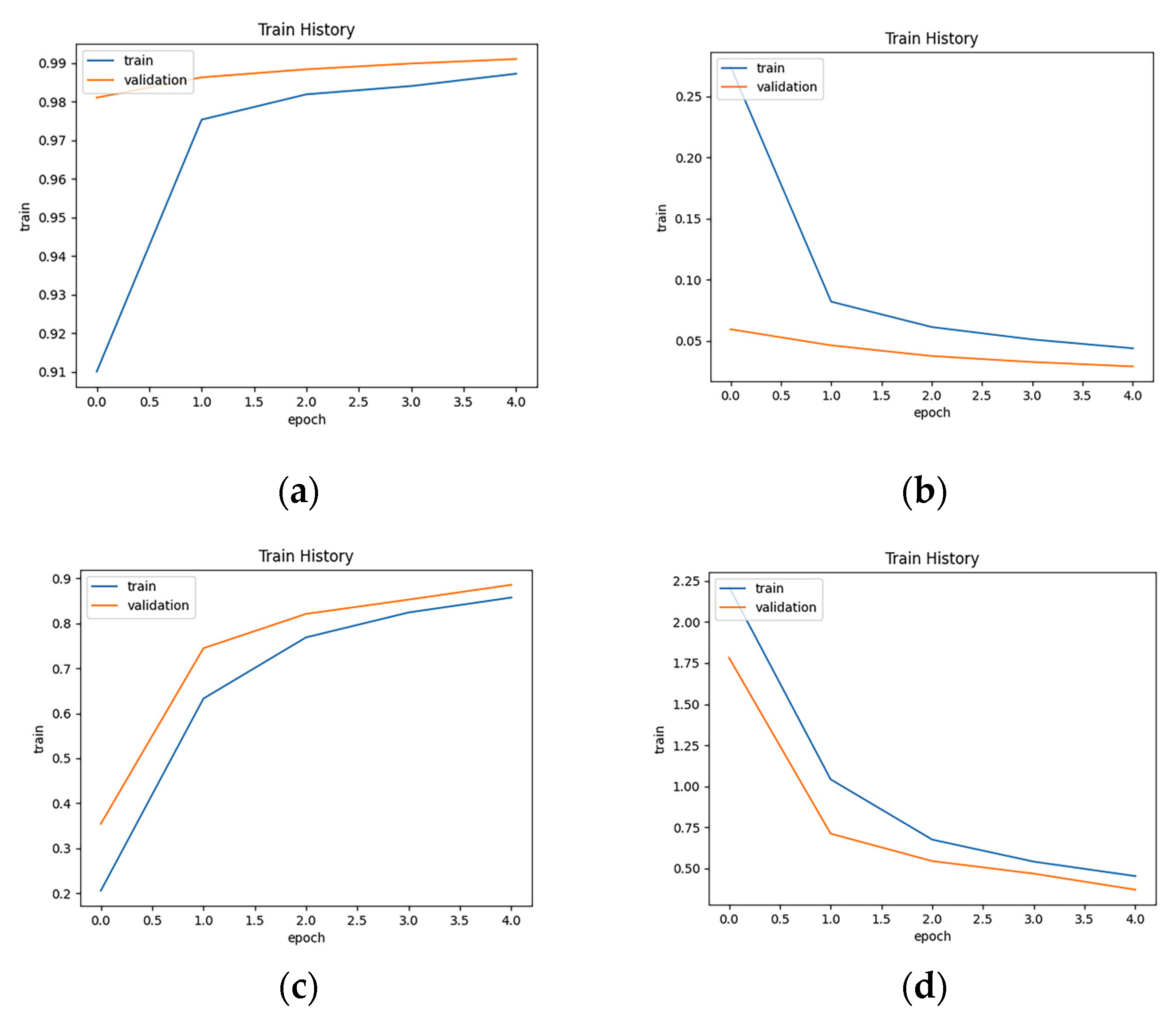
After several experiments, the optimal network fault diagnosis model is finally obtained. Compared with the original CNN model proposed, the average accuracy of the identification and classification of the ship electrical power system is up to 99%. This method makes the fault diagnosis of the ship electrical power system more convenient and reliable. The accuracy and loss variation diagrams were generated using PyCharm and TensorFlow frameworks, as shown in Figure 9a,b, respectively. The accuracy and loss variation diagrams of the original CNN are shown in Figure 9c,d, respectively. The accuracy of each fault category is listed in Table 6.
As can be seen from Figure 9a,b, the overall identification accuracy of the improved model for ship electrical power systems faults increases, and the loss rate decreases as the number of training epochs increases. After the improved model is trained once, the average accuracy of fault diagnosis reaches 97%, and the loss value is less than 0.1. After 4 times of model training, the average accuracy of fault diagnosis is 99%, and the loss value is less than 0.05. A comparison of Figure 9a–d shows that the recognition accuracy of the improved CNN after the first training epoch is higher than that of the original network after four training epochs. At the same time, the convergence speed of the loss value curve of the improved model is higher than that of the original model; the fluctuation range is smaller and is more stable after convergence. As can be seen from Table 6, the accuracy of the improved CNN for different faults at different locations is higher than that of the original network, indicating that the improved CNN provides good classification results for the fault identification of the ship electrical power systems; thus, it has considerable potential for the fault diagnosis of ship electrical power systems.
5. Conclusions
A fault diagnosis method for ship electrical power systems was proposed on the basis of an improved CNN to support the normal operation of ships. According to the results, the following conclusions can be drawn:
- (1)
- To achieve multi-class fault diagnosis of different components of ship electrical power systems, this paper proposed an improved CNN fault diagnosis model, which can completely eliminate the subjectivity of manual feature extraction and expert experience, directly take the original fault data as the model input, automatically extract the fault features layer by layer in a nonlinear manner, and automatically output the fault classification results. Thus, “end-to-end” diagnosis from the original data to the fault category can be realized. The algorithm has a high fault recognition rate, and the evaluation accuracy is 99%.
- (2)
- Through image culling, the accuracy of the network training results is improved significantly.
- (3)
- The method used to realize fault diagnosis of the ship electrical power systems can also be used for fault diagnosis of other parts of more complex power systems. The simulation results showed that the improved model outperforms the original network. In particular, this method achieves high accuracy and reliability in ship electrical power systems fault diagnosis.
Nevertheless, there remains a scope for improvement in terms of the training time of the model. In the future, the simulation model will be improved such that it is more in line with actual ship electrical power systems. Based on the optimized CNN model, fault diagnosis accuracy can be improved further.
Author Contributions
Conceptualization, J.S. (Jie Sun); methodology, C.Y. and J.S. (Jie Sun); software, C.Y. and J.S (Jie Sun); validation, C.J., J.S (Jun Su) and W.S.; formal analysis, J.S. (Jie Sun) and J.S. (Jun Su); investigation, C.Y., J.S. (Jie Sun) and W.S.; resources, J.S. (Jie Sun) and C.J.; data curation, W.S.; writing—original draft, C.Y., L.Q. and J.S. (Jie Sun); writing—review & editing, C.Y. and L.Q.; visualization, J.S. (Jun Su); supervision, L.Q. and C.J.; project administration, L.Q. and C.J. All authors have read and agreed to the published version of the manuscript.
Funding
This research was funded by National Natural Science Foundation of China NO.51875270 and Industry University Research Collaboration of Jiangsu Province NO.BY2020031.
Conflicts of Interest
The authors declare no conflict of interest.
References
- Al-Falahi, M.D.A.; Tarasiuk, T.; Jayasinghe, S.G.; Jin, Z.; Enshaei, H.; Guerrero, J.M. AC Ship Microgrids: Control and Power Management Optimization. Energies 2018, 11, 1458. [Google Scholar] [CrossRef] [Green Version]
- Skjong, E.; Rødskar, E.; Molinas Cabrera, M.M.; Johansen, T.A.; Cunningham, J. The Marine Vessel’s Electrical Power System: From its Birth to Present Day. Proc. IEEE 2015, 103, 2410–2424. [Google Scholar] [CrossRef] [Green Version]
- Yu, C.; Huang, J.; Qi, L.; Gu, J. Health Status Evaluation of Radar Transmitter Based on Fuzzy Comprehensive Evaluation Method. In Proceedings of the 36th Youth Academic Annual Conference of Chinese Association of Automation (YAC), Nanchang, China, 28–30 May 2021; pp. 196–202. [Google Scholar] [CrossRef]
- Maqsood, A.; Oslebo, D.; Corzine, K.; Parsa, L.; Ma, Y. STFT Cluster Analysis for DC Pulsed Load Monitoring and Fault Detection on Naval Shipboard Power Systems. IEEE Trans. Transp. Electrif. 2020, 6, 821–831. [Google Scholar] [CrossRef]
- Ellefsen, A.L.; Æsøy, V.; Ushakov, S.; Zhang, H. A Comprehensive Survey of Prognostics and Health Management Based on Deep Learning for Autonomous Ships. IEEE Trans. Reliab. 2019, 68, 720–740. [Google Scholar] [CrossRef] [Green Version]
- Sulligoi, G.; Vicenzutti, A.; Menis, R. All-Electric Ship Design: From Electrical Propulsion to Integrated Electrical and Electronic Power Systems. IEEE Trans. Transp. Electrif. 2016, 2, 507–511. [Google Scholar] [CrossRef]
- Gunes, M.; Dogru, N. Fuzzy Control of Brushless Excitation System for Steam Turbogenerators. IEEE Trans. Energy Convers. 2010, 25, 844–852. [Google Scholar] [CrossRef]
- Jiang, Y.; Luo, J. The Excitation Switching Control Method of Tidal Generator Based on T-S Fuzzy Weighting. J. Coast. Res. 2020, 103, 1010. [Google Scholar] [CrossRef]
- Jiao, N.; Liu, W.; Meng, T.; Peng, J.; Mao, S. Detailed Excitation Control Methods for Two-Phase Brushless Exciter of the Wound-Rotor Synchronous Starter/Generator in the Starting Mode. IEEE Trans. Ind. Appl. 2017, 53, 115–123. [Google Scholar] [CrossRef]
- Psillakis, H.E.; Alexandridis, A.T. Coordinated Excitation and Static Var Compensator Control with Delayed Feedback Measurements in SGIB Power Systems. Energies 2020, 13, 2181. [Google Scholar] [CrossRef]
- Baek, S.M. Sensitivity Analysis Based Optimization for Linear and Nonlinear Parameters in AVR to Improve Transient Stability in Power System. Int. J. Control. Autom. 2015, 8, 69–80. [Google Scholar] [CrossRef]
- Zhao, H.; Guo, C.; Wu, Z. Modeling and Simulation of marine electric propulsion system. China Shipbuild. 2006, 47, 51–56. [Google Scholar]
- Jardine, A.; Lin, D.; Banjevic, D. A review on machinery diagnostics and prognostics implementing condition-based maintenance—ScienceDirect. Mech. Syst. Signal Processing 2006, 20, 1483–1510. [Google Scholar] [CrossRef]
- Liu, R.; Yang, B.; Zio, E.; Chen, X. Artificial intelligence for fault diagnosis of rotating machinery: A review. Mech. Syst. Signal Processing 2018, 108, 33–47. [Google Scholar] [CrossRef]
- Silva, A.A.; Gupta, S.; Bazzi, A.M.; Ulatowski, A. Wavelet-based information filtering for fault diagnosis of electric drive systems in electric ships. ISA Trans. 2017, 78, 105–115. [Google Scholar] [CrossRef] [PubMed]
- Liu, W.; Liu, L.; Chung, I.Y.; Cartes, D.A.; Zhang, W. Modeling and detecting the stator winding fault of permanent magnet synchronous motors. Simul. Model. Pract. Theory 2012, 27, 1–16. [Google Scholar] [CrossRef]
- Wang, W.; Xu, Z.; Tang, R.; Li, S.; Wu, W. Fault Detection and Diagnosis for Gas Turbines Based on a Kernelized Information Entropy Model. Sci. World J. 2014, 2014, 617162. [Google Scholar] [CrossRef] [Green Version]
- Li, Z.; Jiang, Y.; Duan, Z.; Peng, Z. A new swarm intelligence optimized multiclass multi-kernel relevant vector machine: An experimental analysis in failure diagnostics of diesel engines. Struct. Health Monit. 2018, 17, 1503–1519. [Google Scholar] [CrossRef]
- Cuculić, A.; Vučetić, D.; Prenc, R.; Ćelić, J. Analysis of Energy Storage Implementation on Dynamically Positioned Vessels. Energies 2019, 12, 444. [Google Scholar] [CrossRef] [Green Version]
- Szczerba, Z. Automatic voltage regulator in power generation unit. Przeglad Elektrotechniczny 2009, 85, 55–57. [Google Scholar]
- Ju, P. Theory and Method of Power System Modeling; Science Press: Beijing, China, 2010. [Google Scholar]
- Gao, H.; Hu, X.; Wang, B.; Qi, H. Decentralized Fuzzy PID Excitation controller Combined with Turbine Regulating for Voltage Stability in Power Systems. Prz. Elektrotechniczny 2012, 88, 284–288. [Google Scholar]
- Yee, S.K.; Milanovic, J.V.; Hughes, F.M. Overview and Comparative Analysis of Gas Turbine Models for System Stability Studies. IEEE Trans. Power Syst. 2008, 23, 108–118. [Google Scholar] [CrossRef]
- Kim, H.; Degner, M.W.; Guerrero, J.M.; Briz, F.; Lorenz, R.D. Discrete-Time Current Regulator Design for AC Machine Drives. IEEE Trans. Ind. Appl. 2010, 46, 1425–1435. [Google Scholar]
- Ji, H.-K.; Wang, G.; Kil, G.-S. Optimal Detection and Identification of DC Series Arc in Power Distribution System on Shipboards. Energies 2020, 13, 5973. [Google Scholar] [CrossRef]
- Jeon, W.; Wang, Y.P.; Jeong, J.H.; Lyu, S.K.; Jung, S.Y. Power Characteristic Analysis of Assumed Short Circuit Instance of Electric Ship Propulsion System. Korea Ocean. Eng. Soc. 2008, 32, 323–329. [Google Scholar]
- Martín, S.S.; Fernández, M.B. Model and performance simulation for overcurrent relay and fault-circuit-breaker using Simulink. Int. J. Electr. Eng. Educ. 2006, 43, 80–91. [Google Scholar] [CrossRef]
- Huang, J.; Qi, L.; Gu, J.; Lu, Z.; Sun, J.; Yu, C. Servo Motor Fault Diagnosis Based on Data Fusion. In Proceedings of the 33rd Chinese Control and Decision Conference (CCDC), Kunming, China, 22–24 May 2021; pp. 104–110. [Google Scholar] [CrossRef]
- Guo, Y.; Chen, Y.; Tan, M.; Jia, K.; Chen, J.; Wang, J. Content-aware convolutional neural networks. Neural Netw. 2021, 143, 657–668. [Google Scholar] [CrossRef]
- Arulmozhi, P.; Abirami, S. DSHPoolF: Deep supervised hashing based on selective pool feature map for image retrieval. Vis. Comput. 2021, 37, 2391–2405. [Google Scholar] [CrossRef]
Figure 1.
Excitation control system simulation model.

Figure 2.
Turbine simulation model.

Figure 3.
Discrete frequency regulator simulation model.

Figure 4.
Ship electrical power system simulation model.

Figure 5.
Response curve of single-phase short-circuit grounding fault at synchronous generator terminal.
Figure 5.
Response curve of single-phase short-circuit grounding fault at synchronous generator terminal.

Figure 6.
Response curve of five different faults at synchronous generator end.

Figure 7.
CNN structure.

Figure 8.
Algorithm flow.

Figure 9.
Experimental results of training network and original network: (a) accuracy of training network, (b) loss of training network, (c) accuracy of original network and (d) loss of original network.
Figure 9.
Experimental results of training network and original network: (a) accuracy of training network, (b) loss of training network, (c) accuracy of original network and (d) loss of original network.


Table 1.
Simulation parameters of synchronous generator.
| Parameter | Value |
|---|---|
| 1560 kVA | |
| 480 V | |
| 0.8 | |
| 60 Hz | |
| Polar logarithm, p | 2 |
| 0.022 (pu) | |
| 2.49 (pu) | |
| 1.22 (pu) | |
| 0.15 (pu) | |
| 0.17 (pu) | |
| 0.19 (pu) | |
| 4.4754 | |
| 0.0667 | |
| 0.1 |
Table 2.
Simulation parameters of asynchronous generator.
| Parameter | Value |
|---|---|
| 750 kVA | |
| 480 V | |
| 0.8 | |
| 60 Hz | |
| Polar logarithm, p | 2 |
| 0.022 (pu) | |
| 0.11 (pu) | |
| 0.021 (pu) | |
| 0.11 (pu) | |
| 3.7 (pu) |
Table 3.
Schematic diagram of faults.
| Faults Type | Schematic Diagram |
|---|---|
| Single-phase short-circuit grounding |  |
| Two-phase short circuit |  |
| Two-phase short-circuit grounding |  |
| Three-phase short circuit |  |
| Single-phase disconnection |  |
| Two-phase disconnection |  |
Table 4.
The parameters of the CNN.
| Network Layer | Input | Filter | Output |
|---|---|---|---|
| Conv 0 | |||
| Maxpooling 0 | |||
| Conv 1 | |||
| Maxpooling 1 | |||
| Conv 2 | |||
| Conv 3 | |||
| Maxpooling 2 | |||
| FC 1 | |||
| FC 2 |
Table 5.
The parameters of the improved CNN.
| Network Layer | Input | Filter | Output |
|---|---|---|---|
| Conv 0 | |||
| Maxpooling 0 | |||
| Conv 1 | |||
| Maxpooling 1 | |||
| Conv 2 | |||
| Conv 3 | |||
| Maxpooling 2 | |||
| FC 1 | |||
| FC 2 |
Table 6.
Accuracy of each fault category.
| Fault Category | Fault Location | Improved CNN | CCN |
|---|---|---|---|
| Single-phase short-circuit grounding | Synchronous generator | 99% | 90% |
| Asynchronous generator | 99% | 86% | |
| Main load | 98% | 91% | |
| Secondary load | 99% | 86% | |
| Two-phase short- circuit | Synchronous generator | 99% | 87% |
| Asynchronous generator | 99% | 90% | |
| Main load | 99% | 91% | |
| Secondary load | 98% | 88% | |
| Two-phase short-circuit grounding | Synchronous generator | 98% | 90% |
| Asynchronous generator | 99% | 90% | |
| Main load | 99% | 87% | |
| Secondary load | 99% | 91% | |
| Three-phase short circuit | Synchronous generator | 99% | 86% |
| Asynchronous generator | 98% | 87% | |
| Main load | 99% | 85% | |
| Secondary load | 99% | 88% | |
| Single-phase disconnection | Synchronous generator | 99% | 86% |
| Asynchronous generator | 99% | 89% | |
| Main load | 98% | 90% | |
| Secondary load | 99% | 88% | |
| Two-phase disconnection | Synchronous generator | 98% | 90% |
| Asynchronous generator | 98% | 87% | |
| Main load | 99% | 91% | |
| Secondary load | 99% | 87% |
Publisher’s Note: MDPI stays neutral with regard to jurisdictional claims in published maps and institutional affiliations. |
© 2022 by the authors. Licensee MDPI, Basel, Switzerland. This article is an open access article distributed under the terms and conditions of the Creative Commons Attribution (CC BY) license (https://creativecommons.org/licenses/by/4.0/).
Share and Cite
MDPI and ACS Style
Yu, C.; Qi, L.; Sun, J.; Jiang, C.; Su, J.; Shu, W. Fault Diagnosis Technology for Ship Electrical Power System. Energies 2022, 15, 1287. https://0-doi-org.brum.beds.ac.uk/10.3390/en15041287
AMA Style
Yu C, Qi L, Sun J, Jiang C, Su J, Shu W. Fault Diagnosis Technology for Ship Electrical Power System. Energies. 2022; 15(4):1287. https://0-doi-org.brum.beds.ac.uk/10.3390/en15041287
Chicago/Turabian StyleYu, Chaochun, Liang Qi, Jie Sun, Chunhui Jiang, Jun Su, and Wentao Shu. 2022. "Fault Diagnosis Technology for Ship Electrical Power System" Energies 15, no. 4: 1287. https://0-doi-org.brum.beds.ac.uk/10.3390/en15041287
Note that from the first issue of 2016, this journal uses article numbers instead of page numbers. See further details here.