Article

Estimation of Grid Reinforcement Costs Triggered by Future Grid Customers: Influence of the Quantification Method (Scaling vs. Large-Scale Simulation) and Coincidence Factors (Single vs. Multiple Application)

Energy Network Technologies, Montanuniversitaet Leoben, 8700 Leoben, Austria
*
Author to whom correspondence should be addressed.
Submission received: 15 December 2021 / Revised: 7 February 2022 / Accepted: 11 February 2022 / Published: 14 February 2022
(This article belongs to the Special Issue Power System Planning and Quality Control)

Abstract

:
The integration of future grid customers, e.g., electric vehicles, heat pumps, or photovoltaic modules, will challenge existing low-voltage power grids in the upcoming years. Hence, distribution system operators must quantify future grid reinforcement measures and resulting costs early. On this account, this work initially evaluates different methods to quantify future grid reinforcement needs, applied by the current state of research. Thereby, it indicates the significance of large-scale grid simulations, i.e., simulating several thousand low-voltage grids, to quantify grid reinforcements accurately. Otherwise, a selected area’s total grid reinforcement costs might be misjudged significantly. Due to its fast application, deterministic grid simulations based on coincidence factors are most commonly used in the current state of research to simulate several thousand grids. Hence, in the second step, recent studies’ approaches to applying grid customers’ coincidence factors are evaluated: While simplified approaches allow fast simulation of numerous grids, they underestimate potential grid congestion and grid reinforcement costs. Therefore, a fully automated large-scale grid simulation tool is developed in this work to allow the simulation of multiple grids applying grid customers’ coincidence factors appropriately. As a drawback, the applied deterministic framework only allows an estimation of future grid reinforcement costs. Detailed determination of each grid’s grid reinforcement costs requires time-resolved grid simulations.

1. Introduction

Carbon-neutrality has been declared a priority objective on both the European [1] and national level (e.g., in Austria [2]) to mitigate global warming in the upcoming years. This ambitious objective shall be fulfilled, among other things, by the enhancement of renewable energy sources and a transition towards climate-neutral mobility with a high share of battery electric vehicles (EVs) [1]. In addition, the residential sector’s energy efficiency shall be increased, e.g., by implementing residential electric heat pumps (HPs) [1,3]. While these transitions will reduce the traffic, energy, and residential sector’s carbon footprint, they require integrating numerous new grid customers into the existing power system. The majority (in number) of EVs, photovoltaic modules (PVMs), and electric HPs will be connected to the low-voltage (LV) level [4,5].
As a result, these trends will unquestionably challenge existing LV grids in the following years [6,7,8]. However, future power system structures are planned and designed several decades in advance [9]. Hence, distribution system operators (DSOs) pursue quantifying future grid reinforcement measures (and resulting costs) in their service area at an early stage [9,10,11]. Besides statistical approaches (e.g., [12]), modern-day grid planning relies on numerical load flow simulations to identify potential grid reinforcement measures caused by voltage violations or thermal congestions [13]. Therefore, future grid customers’ loads must be modeled realistically using real-life information (e.g., type, installed power, and energy demand of grid customers). Grid customers’ loads are then implemented into grid models, modeled based on real-life grid topologies and data (e.g., line length and cross-section area) [14].
However, a DSO’s service area often includes several thousand LV grids. The simulation of several thousand grids requires a significant amount of data and computing resources [15]. For DSOs, both are not always available to the required extent. Consequently, quantifying future grid reinforcement needs in a DSO’s service area, including the applied approach to model grid customers’ loads, must comply with given data- and computing criteria. Nevertheless, since grid reinforcements cause significant investment costs for the public sector, the accuracy of grid simulations must not suffer. On this account, this work evaluates different methods to quantify future grid reinforcement costs, applied in the current state of research (Section 2). Furthermore, recent studies’ approaches to model grid customers’ loads are examined regarding accuracy and computing time.

2. State of Research

While several studies analyze the impacts of EVs, PVMs, and HPs on individual LV grids (e.g., [16,17,18]), the presented work focuses on quantifying future grid reinforcements in a large area, including several thousand LV grids. Therefore, the current state of research uses two different ways (Table 1): Most studies identify future grid restrictions in individually selected, representative grids based on load flow simulations. The selected grids’ results are aggregated and scaled to the whole area of investigation (Section 2.1).
Others perform load flow simulations in all grids in the investigated area. The total amount of grid reinforcement measures equals the sum of all grids’ results (Section 2.2). In the following, recent studies in this field are classified accordingly.

2.1. Simulation of Representative Grid Structures and Scaling of Their Results

In Austria, for example, future costs of grid extension measures have recently been estimated by Oesterreichs Energie [10]. Therefore, grid impacts on the LV level caused by integrating EVs (10 and 30% penetration) and PVMs (increase by factor seven) are identified. Fifteen Austrian DSOs (supplying 87% of Austrian grid customers) participate in this study. From those, a third chose to simulate individually selected, representative LV grids and scale their results to the whole service area. Finally, grid reinforcement costs of each participating DSO are aggregated and scaled to the whole of Austria. Based on this approach, this study predicts total grid reinforcement costs on the Austrian LV level between 0.8–2.2 billion euros by 2030 (in addition to regular capital expenditure).
Vu [19] developed a simulation and optimization model to quantify reinforcement costs on the LV level induced by renewable energy sources and EVs. Therefore, representative LV grids are modeled based on typical real-life network characteristics and simulated. The total grid reinforcement costs (between 11.6–22.2 billion euros) are acquired by scaling simulated grids’ results to the whole of Germany. The study performed by Agora [7] determines the required costs of grid extension measures triggered by a future energy transition in Germany. Therefore, this study assumes 6–45 million EVs and 13–17 GW installed power of electric HPs, supplied by renewable energy sources with 65–88% penetration. Real-life grid data of representative power grids are applied for load flow simulation. Finally, the results of representative grid structures are scaled to the entire area of Germany, which results in total grid reinforcement costs between 19–39 billion euros required on the LV level.
Similarly, two additional German studies performed by the German Energy Agency [20] and the German Ministry of Economics and Technology [5] investigate future grid reinforcement costs of German LV networks. For this purpose, both consider possible scenarios based on network development plans and the German federal states’ objectives and projections. In these studies, grid reinforcement costs of representative grids are determined based on grid simulations to scale their results up to the national LV level: 3.6–4.2 billion euros till 2030 [20] and 4.0–9.6 billion euros till 2032 [5].
Matrose et al. [21] investigated grid reinforcement costs caused by EV charging in five countries. On both the medium-voltage (MV) and LV levels, most representative grids are chosen by experts for grid planning and operation. Grid reinforcement costs are determined using load flow simulations for each selected grid. Finally, the relation between required grid reinforcement costs and the grids’ total grid value (representing an exchange of all grid assets) is determined and scaled to all five countries. About 2% (charging with 3.7 kW) or 3% (11 kW) of the total grid value must be invested in MV and LV grids to avoid grid congestions, considering an EV penetration of 30%
Pudjianto et al. [22] quantified future costs required to integrate PVMs in eleven countries in the EU by 2030 (e.g., Italy, UK). This study creates representative European MV and LV grids based on statistical grid data to perform load flow simulations. Finally, total grid reinforcement costs per generated energy (MV and LV level combined) are derived for each of the eleven countries from the simulated results: Between 9.6–13.4 €/MWh (Italy) and between 14.0 €/MWh (UK).
Similarly, Hartvigsson et al. [23] use statistical grid data to model synthetic LV grids, whose capacity for integrating PVMs is determined using grid simulations. The modeled grids’ results are scaled to the whole of Sweden, the UK, and Germany, to quantify these countries’ total hosting capacity on the LV level: 33 GW (Sweden), 63 GW (UK), 248 GW (Germany). However, this study excludes the calculation of required grid reinforcement costs. Durusut et al. [24] indicated that 15.5 billion ₤ (about 18.6 billion euros) must be invested in the UK power system (LV level only) until 2030 due to an extensive transition towards EVs (8.0 million) and HPs (6.8 million). Therefore, ten representative grid models are developed synthetically based on statistical grid data. Flinn et al. [25] determined the integration costs for PVMs in California, USA (up to 744 $ until 2026). Therefore, the authors selected and investigated 75 representative feeders and extrapolated their results to the rest of California (over 10,000 feeders).
While all the studies mentioned above simulate individually selected grids to scale their results to the area of investigation, they vary in the selection (Section 2.1.1) and the number of representative grids to be simulated (Section 2.1.2).

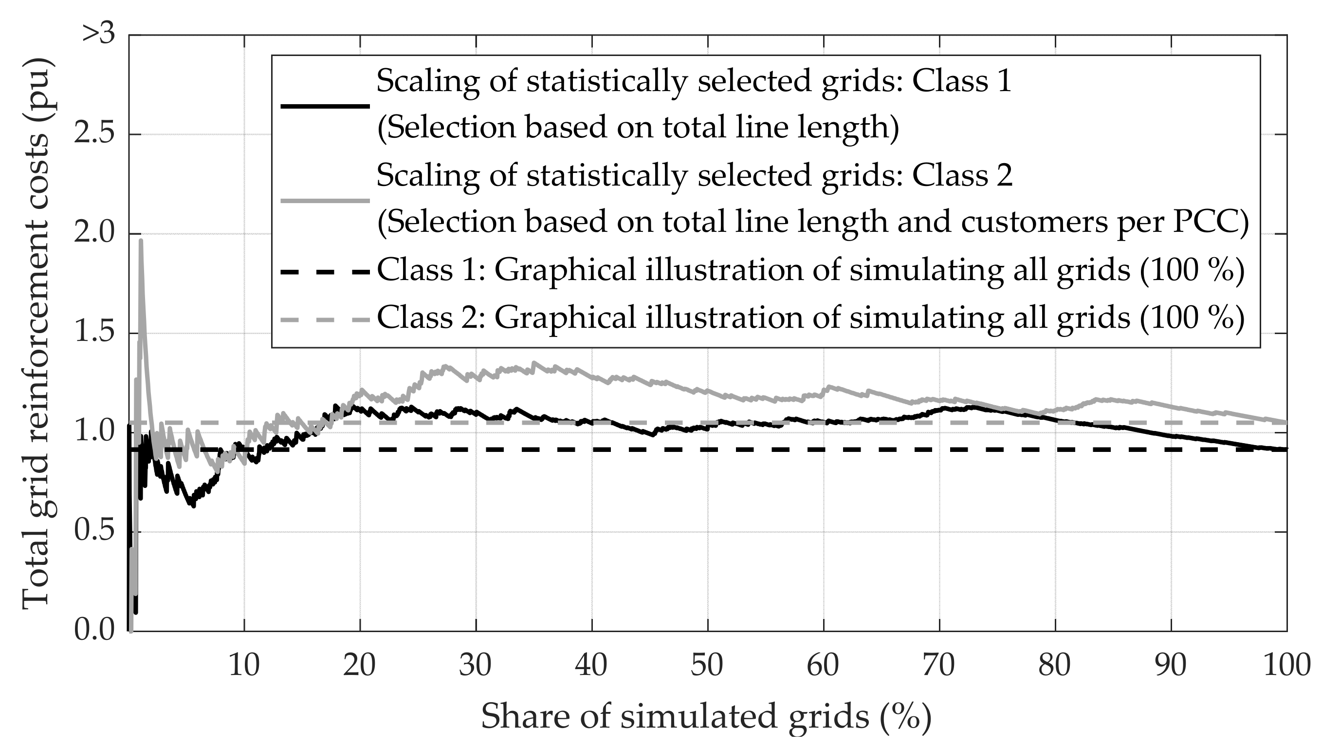
2.1.1. Selection of Representative Grids to Be Simulated

Studies quantifying total grid reinforcement costs by scaling representative grids’ results use different approaches to acquire appropriate grids (Table 1). Four recent studies [5,19,22,23,24] synthetically model representative grids based on real-life grid data and apply them for simulation. Others [7,10,20,21,25] select real-life representative grids to be simulated from all grids in the area of investigation. Therefore, they rely on the experience and insights of experts in the operating and planning of grids.
However, recent studies analyzing total grid reinforcement costs in whole Germany [5,7,19,20] classify German LV grids into, e.g., eleven [20], 18 [5] or 238 [19], representative classes depending on their grid region, topology, or future trends towards renewable energy sources (Table 1). Thus, the scaling of simulated grids’ results is initially done for each class to scale each class’s results to the whole of Germany. Nevertheless, classifying several grids into representative classes requires time-consuming pre-processing, enormous amounts of data, and significant computing effort [15].

2.1.2. Number of Representative Grids to Be Simulated

From all the studies using the described scaling method, only five define the exact number of representative grids to be simulated: The German Ministry of Economics and Technology [5] modeled over two million representative grids synthetically to perform load flow simulations. Pudjianto et al. [22], Hartvigsson et al. [23], and Durusut et al. [24] simulated only 15, 373 and ten synthetically created LV grids, respectively.
In total (considering all representative grid classes), 177 representative LV grids are selected by the German Energy Agency [20] to perform load flow simulation. Matrose et al. [21] and Flinn et al. [25] performed grid simulations in 200 and 75 selected grids, respectively. The remaining works [7,10,19] did not provide this information.

2.2. Large-Scale Grid Simulation of Numerous Real-Life Grid Models

Studies in the second group each simulate several thousand real-life LV grids in the area of investigation to quantify its total grid reinforcement costs. Gupta et al. [6] determined grid impacts of future solar PVMs (20–70% penetration), HPs (up to 100%), and EVs (15–100%) on the LV level, considering the service area of one Swiss DSO. Therefore, the authors perform load flow simulations in 5879 MV/LV substations using GIS data. The authors conclude that by 2050 the total grid reinforcement costs can amount to 11.0 billion CHF (about 10.1 billion euros).
As described in Section 2.1, fifteen Austrian DSOs quantify their grid reinforcement costs by 2030 in the study by Oesterreichs Energie [10]. In contrast to the ones already described, six DSOs perform load flow simulations in all their LV grids to determine required grid reinforcement measures. Lemmens et al. [26] developed a large-scale grid simulation tool to quantify future grid reinforcement measures caused by three different penetrations of EVs and PVMs. Therefore, Flemish LV grids, including 60,000 km grid lines, are simulated and examined regarding voltage violations and thermal congestions. Considering penetrations of 14.4% (PVM), 7.7% (plug-in hybrid EV), and 6.7% (EV), 15,900 km of grid lines (26.5%), and 8% of all transformers must be exchanged.

2.3. Applied Approaches to Modeling Grid Customers’ Load

Besides the applied quantification method, recent studies use different approaches to model future grid customers’ loads as the basis for grid simulations (Table 2): Durusut et al. [24] neglected to specify the applied modeling approach. In only one study [22], grid customers’ loads are taken into account using time series. Three recent studies [5,19,21] use the Monte-Carlo method to stochastically determine the power at each grid node based on statistical data. However, based on its stochastic nature, the Monte-Carlo method requires multiple iterations to be simulated [27]. In contrast to time series-based and Monte-Carlo simulations, static deterministic grid simulations analyze only one load case, which aims to represent the worst-case in terms of grid impacts [28,29]. Therefore, grid customers’ loads are estimated using coincidence factors. Considering a defined number of grid customers ( N o C ), the coincidence factor represents the maximum of their aggregated electrical power ( P i ) divided by the sum of their individual maximum power (Equation (1)) [6,28].
The coincidence factor takes temporal interdependences between grid customers’ electrical loads into account. Thus, it also indicates the probability of simultaneously occurring electrical loads considering a defined number of grid customers: The higher the coincidence factor, the higher the probability of temporal aggregations between grid customers’ loads. Naturally, the more customers are considered, the lower the probability of temporal peak load aggregations and the lower the coincidence factor [30]:
C o i n c i d e n c e   f a c t o r N o C = max t ( i = 1 N o C P i t ) i = 1 N o C max t P i t
Since it only requires one time step to be simulated, the application of coincidence factors allows much faster computation [27,31] than time series-based and Monte-Carlo simulations. That is why most studies analyzing many real-life grids [6,7,10,20,23,26] use this approach (Table 2).
However, since the coincidence factor depends on the number of considered customers, it must be adapted according to the grid element to be analyzed: Grid elements supplying numerous customers (e.g., the MV/LV substation) are characterized by low coincidence factors. In contrast, grid elements supplying few customers (e.g., grid lines at the end of feeders) are characterized by high coincidence factors. Nevertheless, recent studies use various approaches to applying grid customers’ coincidence factors. Hence, they consider this aspect differently:
Hartvigsson et al. [23] and Gupta et al. [6] determined one single coincidence factor specifically for each grid based on the number of grid customers supplied by the MV/LV substation (Figure 1). This single value is applied to each grid customer to perform load flow simulations. The German Energy Agency [20] and Flinn et al. [25] also apply one single coincidence factor to each grid customer. Although, these studies use a consistent coincidence factor for each LV grid to be simulated, neglecting the grid’s actual number of customers. Lemmens et al. [26] applied one single coincidence factor to each grid customer. Therefore, the number of customers supplied by the respective feeder’s main line (Figure 1) is considered for each grid specifically.
In contrast to the previous works, the studies performed by Oesterreichs Energie [10] and Agora [7] apply two different coincidence factors to each grid customer depending on the grid element to be analyzed. The coincidence factor applied to analyze the MV/LV substation is determined based on the total number of customers the substation supplies. For a second load flow simulation, the number of customers supplied by each feeder’s main line is used to define the coincidence factor for all remaining elements in the respective feeder. Both coincidence factors are varied for each LV grid specifically.
In conclusion, recent studies’ approaches to applying coincidence factors differ regarding the following aspects (Table 2): Firstly, the coincidence factor’s variation in the analyzed grids (consistent or defined for each grid specifically). Secondly, the number of various coincidence factors applied to each grid (single or multiple). Thirdly, the grid element on the basis of which the coincidence factors are determined (MV/LV substation or each feeder’s main line). By applying one single coincidence factor to each grid customer (e.g., defined based on the number of customers the MV/LV substation supplies), numerous grid elements might be examined using inappropriate coincidence factors. As a countermeasure, multiple coincidence factors must theoretically be applied to grid customers to analyze each grid element adequately. However, recent studies determining total grid reinforcement costs in several thousand grids include this aspect differently due to different approaches to applying coincidence factors.

2.4. Remaining Gap in the Current State of Research

Previous sections indicate different methods to quantify grid reinforcement needs (Section 2.1 and Section 2.2) and model grid customers’ electrical loads (Section 2.3) applied in recent studies. This broad spectrum of methods and simplifications impedes comparing recent works in this field and their results [32]. Indeed, Vu [19] demonstrated significant differences (about 21–45% concerning the total line length to be reinforced in Germany) between the presented study and the ones performed by the German Energy Agency [20] and the German Ministry of Economics and Technology [5].
Identifying the impact of the selected quantification method (scaling of representative grids’ result or large-scale grid simulations) and the approach to model grid customers’ electrical loads (consistent or grid-specific, single or multiple) would facilitate the comparison of studies in this field. To the authors’ best knowledge, only one study addresses this issue: Eberl et al. [15] have analyzed different methods (e.g., [19,20]) to quantify grid reinforcement costs in a large area with several thousand grids. However, those methods are evaluated only qualitatively regarding the accuracy of results, assumptions and simplifications, and the required amount of data.
The shortage of applying only one single coincidence factor for all grid customers has been quantified in 13 LV grids by Ulffers et al. [33]. Nevertheless, the current state of research lacks a quantitative analysis of how recently applied methods and approaches can affect the calculated grid reinforcement costs in a large area with several thousand grids [32].

3. Open Research Questions and Structure of This Work

Based on the remaining gap in the current state of research (Section 2.4), the following research questions remain unsolved:
(1)
What is the potential error when simulating only a few individually selected LV grids and scaling their results to quantify grid reinforcement costs in a large area?
(2)
How many grids (in %) must be simulated to reach a certain degree of accuracy?
(3)
How to apply grid customers’ coincidence factors to quantify grid reinforcement measures accurately (consistent or grid-specific; single or multiple; based on which grid element)?
(4)
What is the trade-off between the acquired simulation accuracy and required computing time?
(5)
How to quantify future grid reinforcement costs allowing both high accuracy and adequate computing time in the most optimal way?
Various quantification methods and approaches to applying coincidence factors, used in the current state of research, are analyzed to answer these research questions for one DSO’s service area with several thousand LV grids. Therefore, an automated large-scale grid simulation tool is developed (Section 4.1) and applied to quantify future grid reinforcement needs using real-life grid data (Section 4.2). The investigated scenario regarding the penetration of EVs, PVMs, and HPs is described in Section 4.3. Section 4.4 and Section 4.5 demonstrate the evaluated quantification methods and approaches to applying coincidence factors. Their impacts on the determined grid reinforcement measures and the required computing time are demonstrated in Section 5. Finally, Section 6 discusses this paper’s results according to the presented research questions and provides an outlook on further work.

4. Materials and Methods

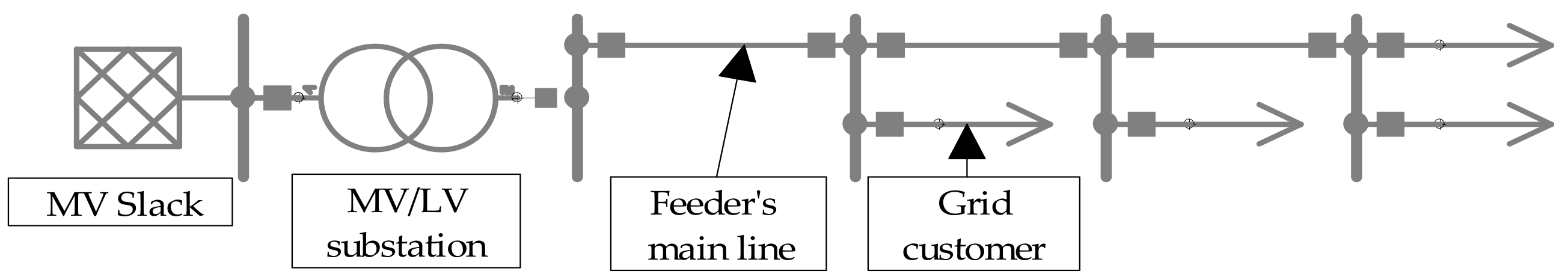
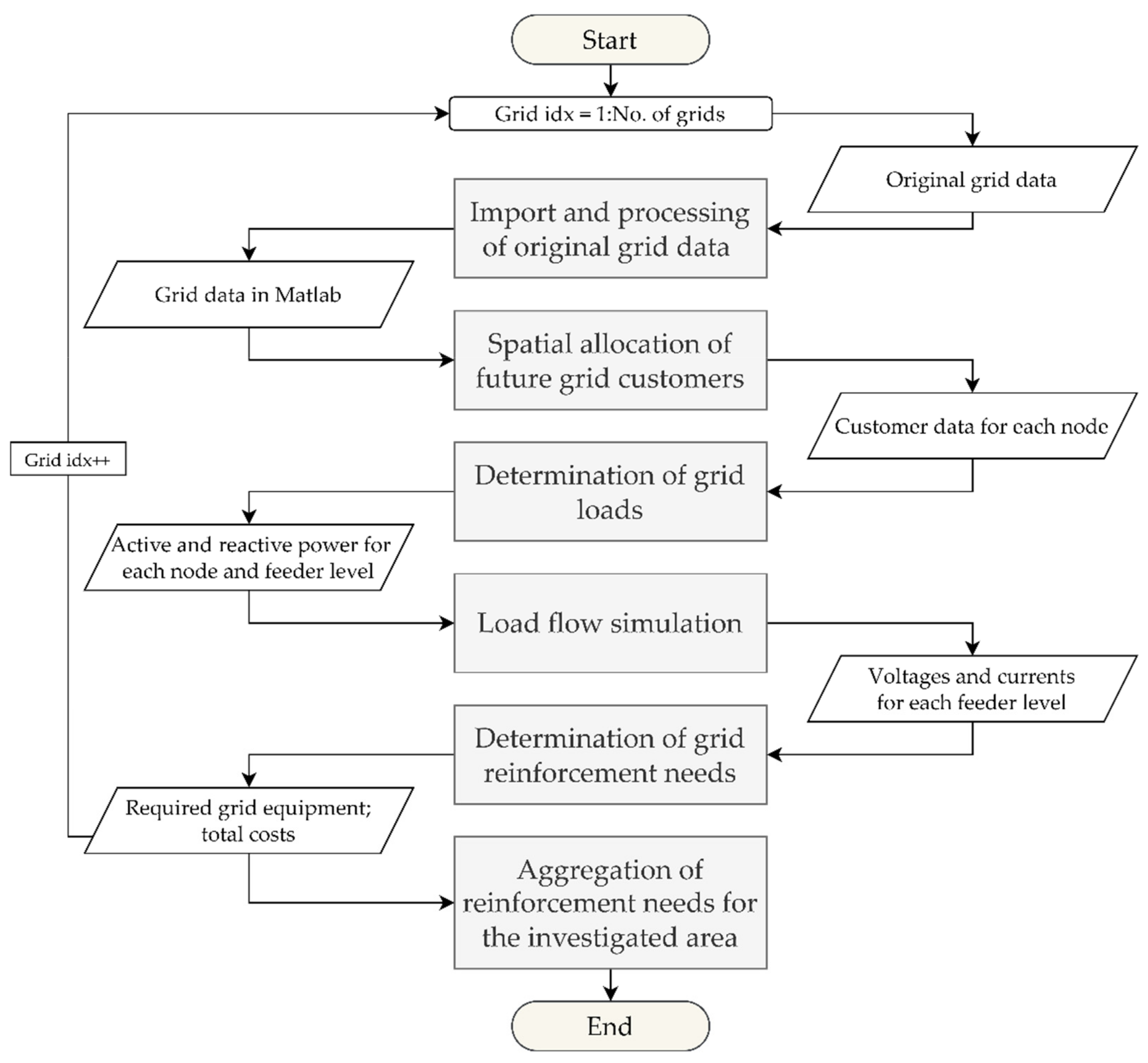
4.1. Automated Large-Scale Grid Simulation Tool: Quantification of Grid Extension Needs

The grid simulation tool developed in this study allows fully automated analysis of several thousand grid models, including evaluating potential grid reinforcement needs. Thereby, all LV grids in a DSO’s service area can be simulated and examined in terms of grid restrictions. The tool’s scheme applied for each grid model respectively is illustrated in Figure 2. The following sections describe each of these steps in detail. The parallelization of the presented scheme (Figure 2) using 32 CPUs (3 GHz, 128 GB RAM) in MATLAB allows the simulation of several grid models simultaneously (one grid model per CPU). Thereby, it enables an average computing time of 20.8 s per 1000 grid nodes, about 16 times faster compared to a sequential simulation.

4.1.1. Import and Processing of Original Grid Data

In the first step of the grid simulation tool, each grid’s original grid data is imported into MATLAB. Therefore, we developed interfaces between commercial grid simulation tools (e.g., NEPLAN [34], PowerFactory [35]), database software (e.g., MS Access), and MATLAB, allowing fully automated and standardized data transfer. For a successful performance of the developed tool, each grid’s data set must include the following information:
  • Power lines and transformers: Maximum current, internal impedance (R’, L’, C’), and connected nodes
  • Grid nodes: Type of node (Slack, PQ, or PV), nominal voltage as well as type (e.g., household, PVMs, EVs, and HPs), number, and installed power of connected grid customers
Each grid’s topology is structured into feeders and feeder levels, as shown in Figure 3. The feeder level represents the distance of grid elements (transformers, nodes, and lines) from the MV slack: The higher the feeder level, the higher the distance. Transformers at the MV/LV substation and the connected LV bus bar are characterized by feeder level 1.
Grid lines and nodes connected to the LV bus bar are assigned feeder level 2. This scheme is continued until all grid elements are assigned a particular feeder level (Figure 3).
Like recent studies simulating several thousand LV grids (Section 2.3), the developed tool uses coincidence factors to model grid customers’ loads. However, the coincidence factor depends on the number of customers considered.
Hence, it must be adapted according to the grid element to be analyzed. The implementation of feeder levels allows us to apply the appropriate coincidence factor to each grid customer depending on the grid element to be analyzed (described in detail in Section 4.1.3).

4.1.2. Spatial Allocation of Future Grid Customers

Besides existing grid customers, the automated large-scale grid simulation tool analyzes future EVs, PVMs, and HPs and their impacts on LV networks. Therefore, the total number of EVs, PVMs, and HPs in each LV grid is determined based on the analyzed penetrations (from 0–100%) and the total number of households (assuming maximally one EV, PVM, and HP per household). While existing grid customers’ location in the grid is documented in the imported grid data (Section 4.1.1), future customers’ spatial allocation is, of course, unclear. The distribution of future grid customers significantly influences their grid impact and on resulting grid reinforcement costs [24]. Therefore, the spatial allocation of EVs, PVMs, and HPs can freely be selected using the automated large-scale grid simulation tool (e.g., stochastic or uniform). As relaxation of the problem, this study assumes a uniform placement of future customers to the grid’s nodes (cf. Thormann et al. (2020) [8]). In the end, this step provides all relevant data regarding existing and future grid customers for each node, which is then applied to determine realistic grid loads (Section 4.1.3).

4.1.3. Determination of Grid Loads

Quantifying grid reinforcement measures requests the identification of critical grid loads and their impacts on the investigated grid. Since the automated large-scale grid simulation tool uses static deterministic grid simulation, critical grid loads are determined using coincidence factors (described in Section 2.3). Considering a certain number of customers ( N o C ), their aggregated power ( P a g g r e g a t e d ) is calculated by multiplying the sum of their individual maximum powers ( P m a x i ) by the respective coincidence factor ( C F ), according to Equation (2) [28]:
P a g g r e g a t e d N o C   =   i = 1 N o C P m a x i ·   C F N o C
The maximum power of existing customers is provided by original grid data (Section 4.1.1). In contrast, future customers’ peak power is defined as follows: The possibility of charging EVs strongly depends on the type of housing, i.e., family houses or multi-apartment residential buildings. Analogously to Thormann et al. [8], this study classifies future EVs accordingly: EVs charged with high power (11 kW) at family houses and EVs charged with low power (3.7 kW) at multi-apartment residential buildings. Additional PVMs are integrated into the grid model with a maximum power of 5 kW (feeding into the grid). The load profile of electric HPs is characterized by increased starting current/power due to the compressor motor [36]. However, since starting currents last only few seconds, a base load of 3.0 kW (cf. [37,38,39]) is assumed for this customer type.
As described in Section 2.3, coincidence factors are applied for load flow simulations to take temporal interdependences between grid customers into account. Besides the number of grid customers, these interdependences depend on the customer types (e.g., households, EVs). While state-of-the-art coincidence factors neglect this aspect, novel coincidence factors have been modeled in the authors’ previous work (Thormann et al. [8], Figure 4). It also describes the methodology applied for modeling these new coincidence factors.
Since the modeled coincidence factors combine different customer types, the coincidence factor at a certain aggregated number of customers varies depending on their distribution. For example, three households are characterized by a lower coincidence factor than one household with one EV and one HP (in total, three customers). In general, EVs and PVMs (near one) are characterized by high coincidence factors, whereas households and HPs are characterized by lower ones (Figure 4). As described in Section 2.3 and demonstrated in Equation (2), the coincidence factor (and the resulting aggregated power) depends on the number of considered customers. Hence, it must be adapted according to the grid element to be analyzed and its number of supplied customers. As a result, static deterministic load flow simulation (one time step only) using coincidence factors does not allow the accurate simulation of all grid elements at once.
Therefore, each LV grid is structured into several feeder levels, described in Section 4.1.1 (Figure 3). The coincidence factor defined at each customer depends on the analyzed grid element, hence, the respective feeder level (Figure 5): When analyzing the MV/LV substation in feeder level 1 (e.g., supplying three customers), the respective coincidence factor (e.g., 0.65) is applied to each connected customer. The aggregated power (13.0 kW), calculated using Equation (2), is distributed to grid customers (6.5, 2.6, and 3.9 kW) according to their maximum individual power (10.0, 4.0, and 6.0 kW).
Each feeder’s main line (Line 1 in Figure 5) is evaluated, considering feeder level 2 (e.g., supplying two customers). Therefore, each connected customer is assigned the respective coincidence factor (e.g., 0.80), whereas non-relevant customers are neglected (coincidence factor of 0.0). This procedure is done for each feeder level. In the end, each customer is assigned one coincidence factor and one power value for each feeder level, respectively (Figure 5). After determining the active power for each grid customer and feeder level, reactive power is calculated by using the following power factors: 0.99 (leading) for EVs, 1.00 for PVMs, and 0.90 (lagging) [8,36,40,41].

4.1.4. Load Flow Simulation

In the next step, active and reactive power values of each customer and each feeder level are applied to analyze potential grid restrictions. Therefore, static load flow simulations are performed using the Newton-Raphson method. For each feeder level, one static load flow simulation is performed using the appropriate coincidence factor for each customer (Figure 5). All grid elements assigned to the same feeder level are analyzed simultaneously. Hence, the number of required load flow simulations equals the number of feeder levels assigned to each grid, respectively. However, the developed grid simulation tool allows users to define the number of simulated feeder levels to adapt to the available computing power. In this study, the number of simulated feeder levels is varied (Section 4.5) to investigate different approaches to applying coincidence factors and their impact on simulation accuracy.
As output data, the static load flow simulation provides each node’s complex voltage ( V _ O u t p u t ; Figure 6a) and the thermal utilization of transformers and lines (Figure 6b) for each simulated feeder level. However, the actual results of individual elements (nodes, transformers, and lines) depend on their actual coincidence factor and, thereby, the assigned feeder level. Thus, the actual current of transformers and lines is retrieved from the output data (Figure 6b) according to their assigned feeder level, e.g., at feeder level 1 for the MV/LV substation or at feeder level 3 for Line 2 (Figure 5).
The actual complex voltage of a node n ( V _ n ,   a c t u a l ) is calculated according to Equation (3), based on the actual complex voltage of the previous node ( V _ n 1 ,   a c t u a l ) and their complex output voltages ( V _ O u t p u t ; Figure 6a) at the feeder level of node n ( F L n ). The applied calculation of voltages can only be used for evaluating radial grid structures, not for mesh networks. However, considering radial grid structures on the LV level, this method has been validated by time series-based grid simulation in Thormann et al. [8]
V _ n ,   a c t u a l = V _ n 1 , a c t u a l + V _ O u t p u t F L n , n V _ O u t p u t F L n , n 1
In the end, the performed load flow simulations provide each node’s actual voltage and the actual current of transformers and lines. The grid’s actual voltages and currents are then applied to evaluate potential grid reinforcement needs (Section 4.1.5).

4.1.5. Determination and Aggregation of Grid Reinforcement Needs

In the final step of the automated large-scale grid simulation tool, required grid reinforcement measures induced by various grid customers (existing ones, EVs, PVMs, and HPs) and resulting costs are determined. Therefore, each grid’s results are examined for voltage violations and thermal congestions (cf. [7,19,20]). The acceptable voltage range and the maximum thermal utilization of transformers and lines are defined freely by the user. The European standard EN 50160 [42] defines the acceptable voltage range of the LV and MV levels with ±10% of the nominal voltage. However, this voltage range is shared by both voltage levels conjunctly. According to the voltage range partitioning presented in [5,43], an acceptable voltage range of [104.5%; 93.5%] of the nominal voltage (0.4 kV) is used in this study. In addition, grid reinforcements are required if transformers or lines exceed their allowed thermal utilization of 100%. Depending on the type of grid restriction, the following grid reinforcement measures are automatically executed in the grid model (cf. [7,20,44]):
  • Thermal overload of the transformer(s) at the MV/LV substation: The developed tool initially examines whether the parallel installation of an additional transformer with the same nominal power as the existing one(s) is sufficient to prevent thermal overload. If not or the maximum number of parallel transformers is already reached (Table 3), existing transformers at the MV/LV substation are exchanged with new ones, providing sufficient nominal power.
  • Thermal overload of individual lines: If individual grid lines are overloaded, additional lines are installed parallel until the maximum power can be transmitted or the maximum number of parallel lines (Table 3) is reached. Therefore, the cable type NAYY 4 × 150 mm2 (cf. [7,20]) with a maximum current of 245 A is installed by default.
  • Voltage violations: If one or more nodes show inadmissible voltages, the affected feeder is divided into two feeders at 2/3 of the total length from the MV/LV substation (cf. [20]).
As a result, this step provides the number and nominal power of additional transformers as well as the total length of additional grid lines to be installed in the grid. Grid reinforcement costs are estimated for each grid by applying specific construction- and material costs of additional transformers and grid lines. While the user can define specific costs freely, this study uses values listed in Table 3, including personnel-, planning- and construction costs [7,20,44].
In the current version of the developed grid simulation tool, measures of congestion management are excluded. However, they will be integrated into further versions of the tool. The developed automated large-scale grid simulation tool executes the workflow described in Section 4.1 (Figure 2) for each grid. All the grids’ costs are aggregated to determine total grid reinforcement measures in the investigated area caused by a user-defined scenario (e.g., characterized by a specific EV-, PVM- and HP-penetration).

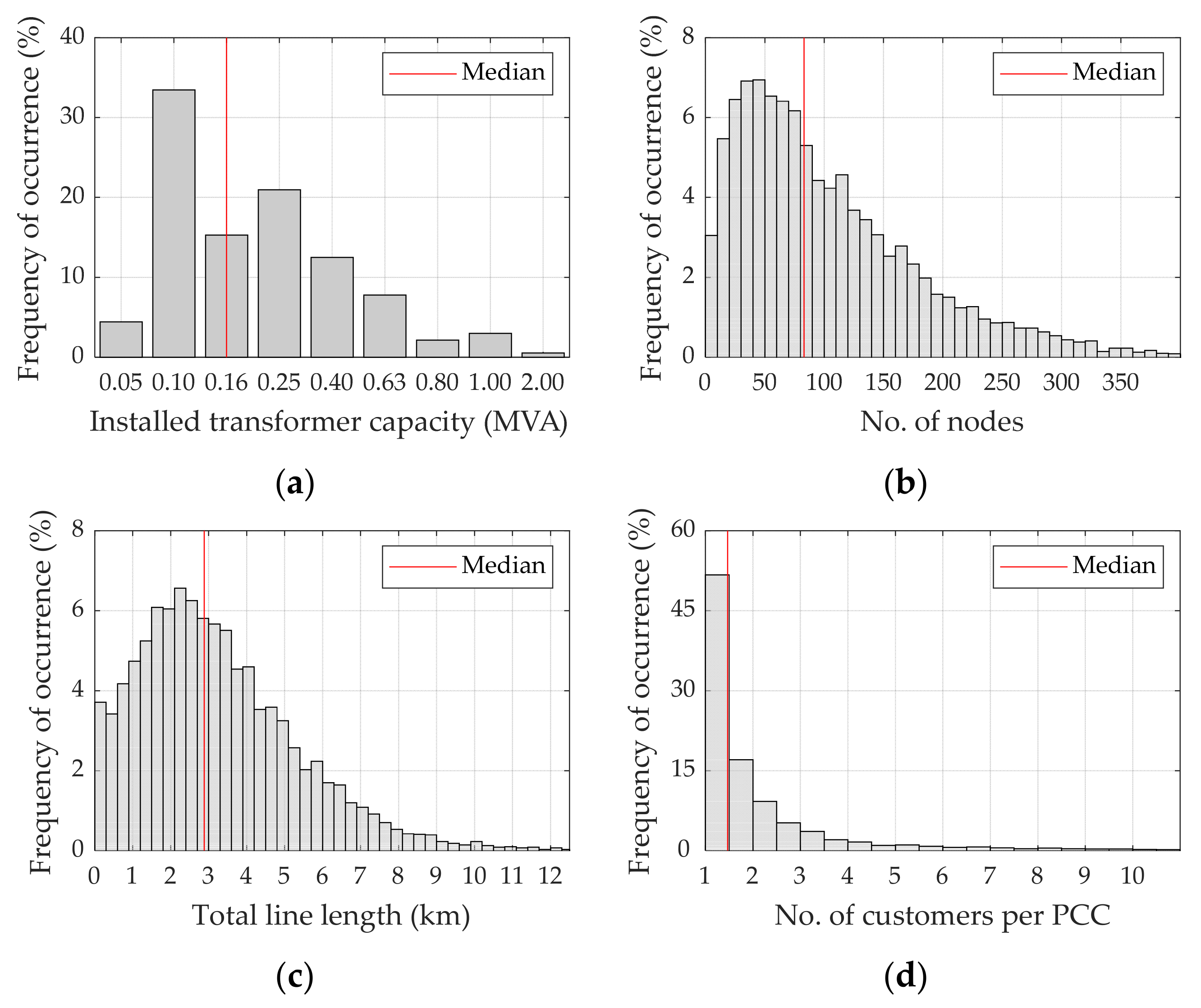
4.2. Grid Data Applied in This Study

This study evaluates various methods and approaches to quantify potential grid reinforcement needs based on 7114 real-life LV grids. The analyzed LV grids are operated by a major Austrian DSO whose service area is mainly characterized by suburban and rural regions. Figure 7 describes the analyzed LV grids by illustrating their frequency of occurrence and median regarding the installed transformer capacity, the number of nodes, the total line length, and the average number of customers per point of common coupling.
Most LV grids are supplied by a MV/LV transformer with a capacity of 0.10 (34%), 0.16 (15%, median), 0.25 (21%), or 400 MVA (13%). Only 13% of MV/LV substations are equipped with a higher transformer capacity (Figure 7a). In total, the investigated LV grids include about 740,400 nodes with a median of 83 nodes per grid (Figure 7b) and 23,000 km of grid lines with a median of 2.89 km (Figure 7c). All grids together supply 498,600 customers via 207,400 points of common coupling. The median of 1.47 customers per point of common coupling (Figure 7d) demonstrates a relatively low population density in the area of investigation.
Grid customers can be classified into 307,200 households (median: 43), 60,300 commercial businesses, 29,800 agricultural businesses, 83,100 electric water heaters, 2000 lighting systems and 16,200 existing PVMs. Each grid is structured as a radial network and supplied by the MV grid (represented by an MV slack node) via one or two MV/LV substations and transformers (Figure 3). In conclusion, the investigated LV grids show a high heterogeneity regarding the installed transformer capacity, the number of nodes, the total line length, and the number of customers per point of common coupling (Figure 7). However, this discrepancy between real-life LV grids has also been noticed in central Europe and the USA due to various grid planning approaches of DSOs and geographical differences [45,46,47,48]. In fact, the statistical distribution of the analyzed LV grids’ parameters shows similarities to other studies (e.g., [49,50,51]).

4.3. Scenario Applied in This Study

Besides the quantification method and the approach to applying coincidence factors, recent studies differ concerning the considered scenarios. In contrast, this work compares those methods and approaches by applying one consistent scenario. Therefore, the future penetration of EVs, PVMs, and HPs is derived for 2030. According to the Environment Agency Austria [52], this study assumes an EV penetration of 27% in 2030. Furthermore, we assume that 30% of households will be equipped with domestic PVMs in 2030, according to Fechner [53]. The future penetration of electric HPs is estimated based on the study by Fraunhofer [54], which predicts their penetration between 14–31% in 2030. Hence, this study uses the mean value of 23% to compare various quantification methods and approaches to applying coincidence factors.

4.4. Varying the Applied Method to Quantify Grid Reinforcement Measures

The presented study evaluates four different methods to quantify grid reinforcement costs (Table 4) in the area of investigation, including 7114 LV grids (Section 4.2). Those follow the methods applied by the current state of research and presented in Section 2. Thereby, they vary in the selection and number of grids to be simulated based on load flow simulations: The first method (Scaling of grid regions) performs load flow simulations selecting three representative LV grids, one per grid region (urban, suburban, and rural according to [55]). As in most recent studies (Section 2.1.1), representative grids are selected in consultation with the respective grid planners and based on their experience and know-how. The total grid reinforcement costs in the selected area are determined by simulating the selected grids and scaling their costs to the whole area (7114 grids) according to Equation (4):
T o t a l   g r i d   r e i n f o r c e m e n t   c o s t s = ( i = 1 N o .   o f   s i m u l a t e d   g r i d s C o s t s i ) ·   7114 N o .   o f   s i m u l a t e d   g r i d s
The second quantification method (scaling of arbitrarily selected grids) randomly selects representative grids from the available grid data to perform grid simulations. Total grid reinforcement costs are then estimated by scaling the grids’ results to the defined area (Equation (4)). This method’s results strongly depend on the number of selected grids and the selected grids’ structures. On this account, we vary the number of simulated grids between 1–7114 using this method (Table 4). For each number of simulated grids, the random selection and simulation of grids are repeated 1000 times to vary the analyzed grid structures as well. Since this method neglects the statistical distribution of grids’ parameters (e.g., transformer capacity, number of nodes, number of customers, total line length), it represents a simplified approach to select grids for simulation.
In contrast, the third quantification method (scaling of statistically selected grids) selects representative grids to be simulated based on statistical data (cf. [46,56]). Therefore, the root mean square relative deviation between each grid’s parameters (installed transformer capacity, number of nodes, total line length, and the number of customers per point of common couplings) and the respective medians (demonstrated in Section 4.2) are calculated. Similar to method 2, the number of simulated grids is varied between 1–7114. For each number of simulated grids, those with the lowest root mean square relative deviation are selected for simulation. The total grid reinforcement costs are calculated by scaling their results to the whole area of investigation (Equation (4)). In the fourth quantification method (simulation of all grids), we simulate all 7114 LV grids in the investigated area, requiring no scaling or grid selection. Total grid reinforcement costs are determined by aggregating all grids’ results.
The developed grid simulation tool (Section 4.1) is applied for each method, though different numbers of grids are simulated (Table 4). Furthermore, all feeder levels are simulated in each quantification method to consider each grid element’s appropriate coincidence factor (approach 4 in Section 4.5).

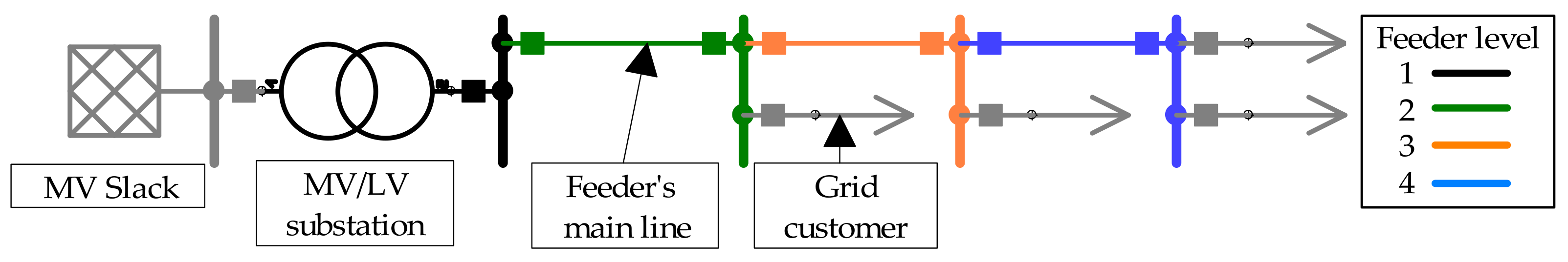
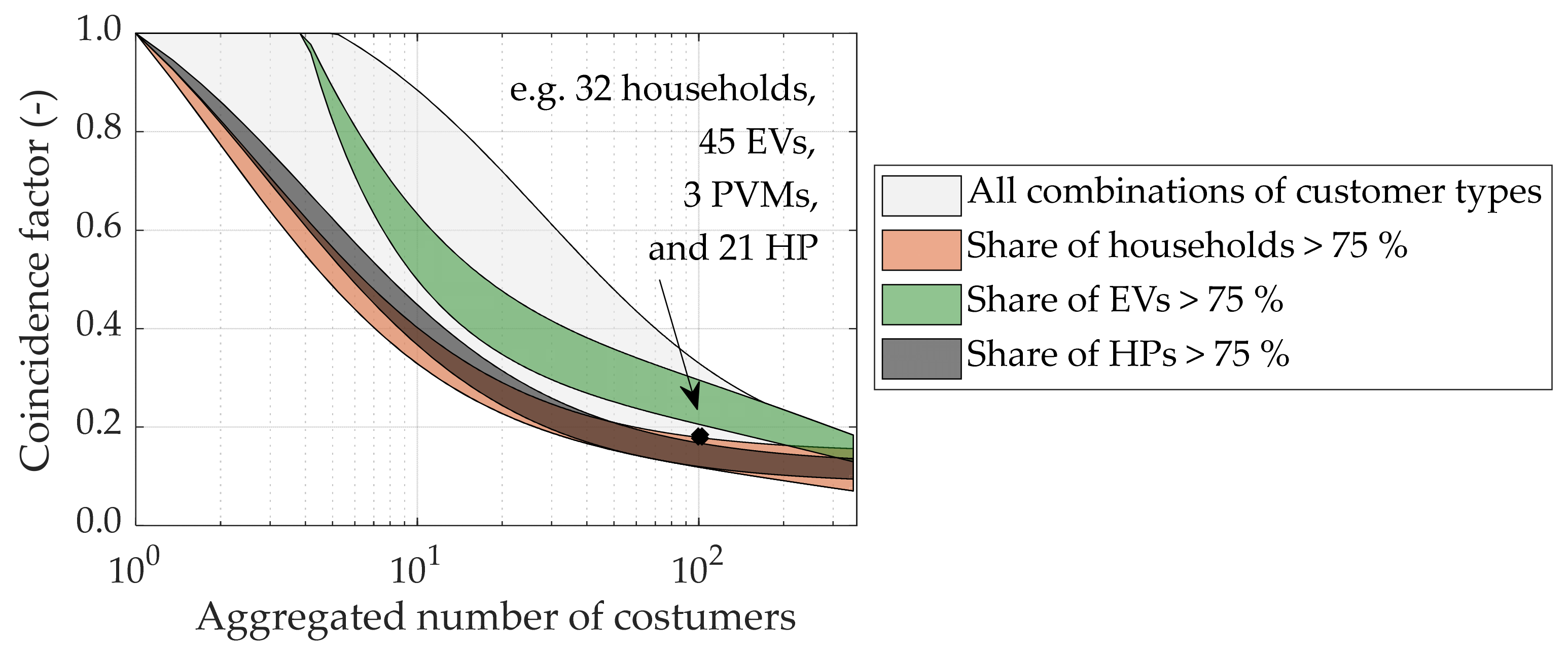
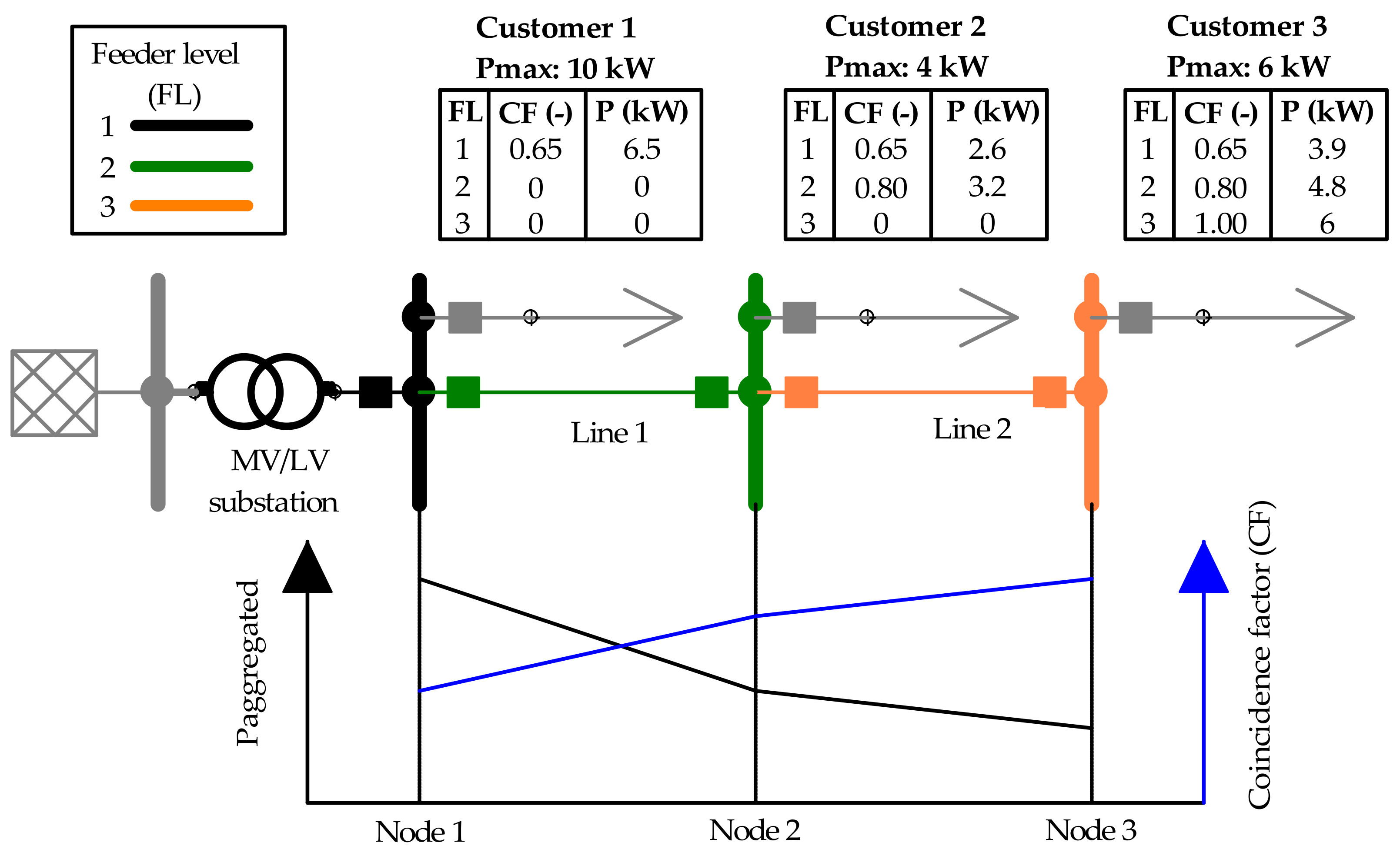
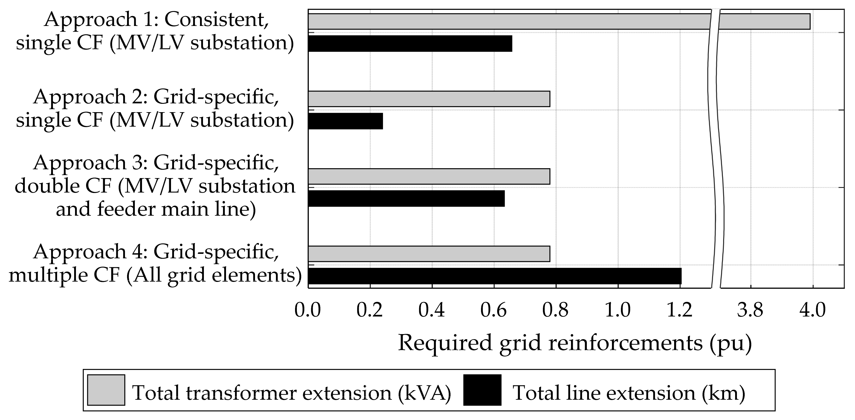
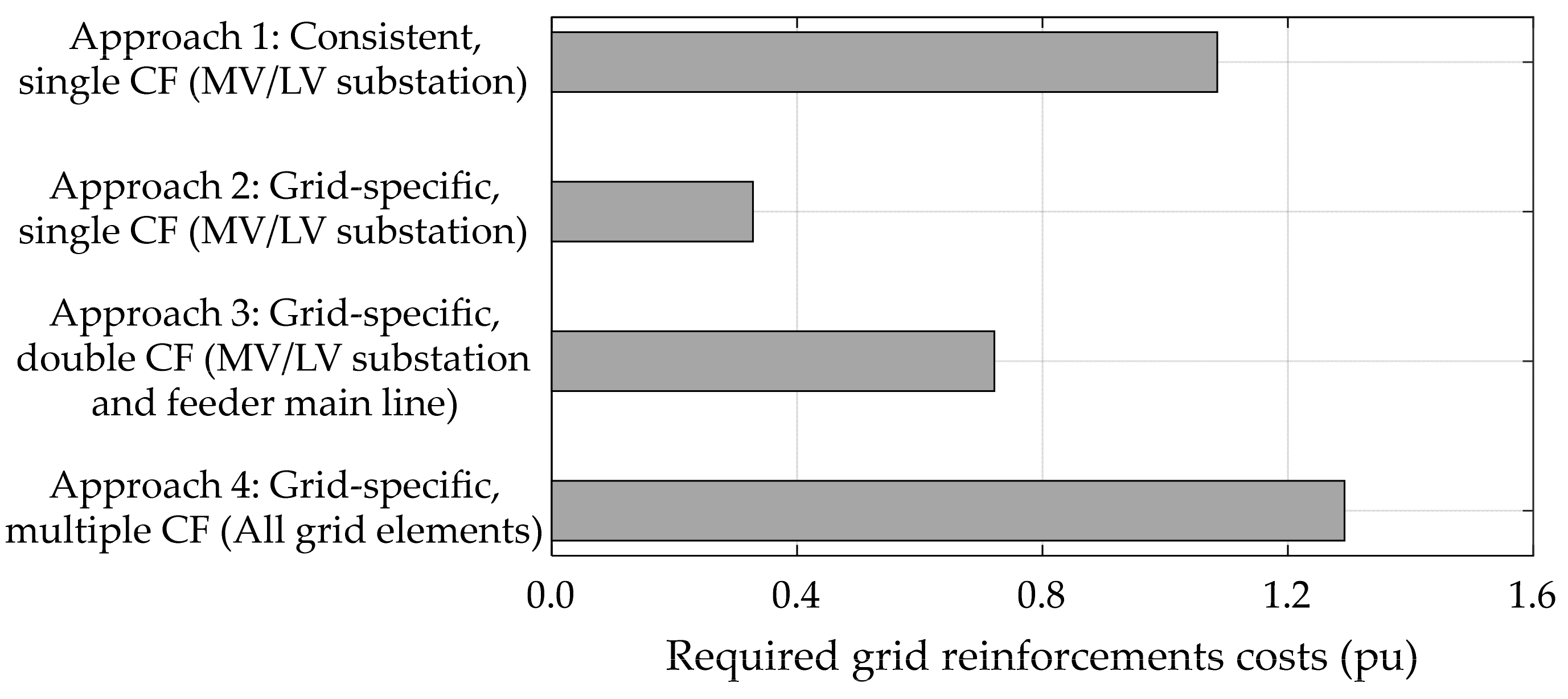
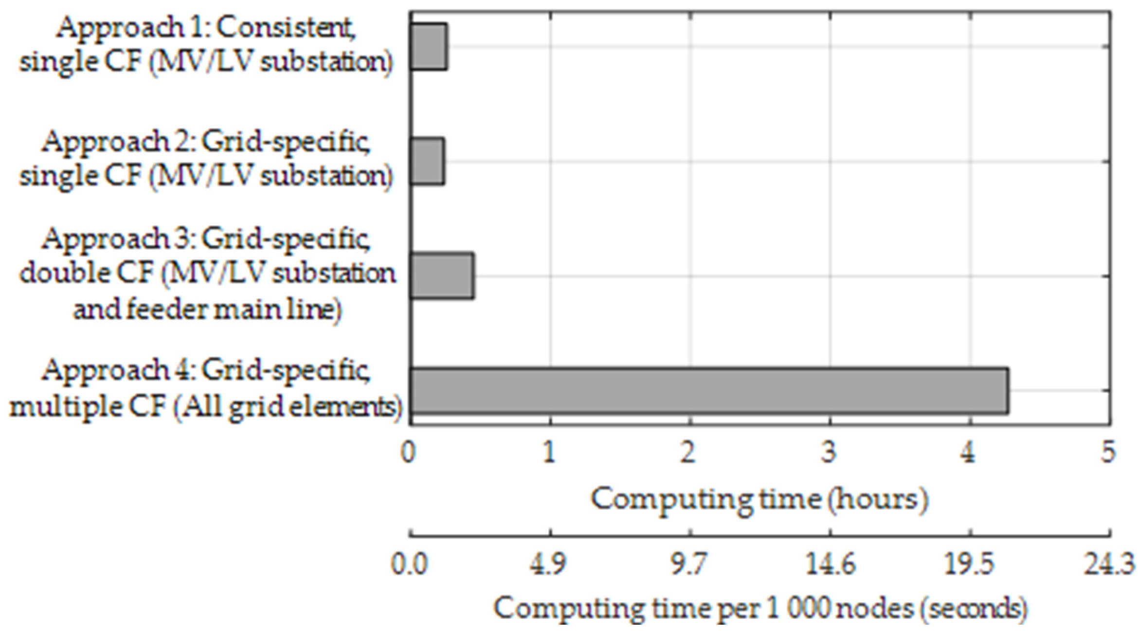
4.5. Varying the Approach to Applying Coincidence Factors

As demonstrated in Section 2.3, studies quantifying future grid reinforcement costs in a large area vary regarding the following aspects:
  • The coincidence factor’s variation in the analyzed grids (consistent or grid-specific)
  • The number of various coincidence factors applied per grid (single or multiple)
  • The grid element on the basis of which the coincidence factors are determined (the MV/LV substation or each feeder’s main line)
The presented study identifies these aspects’ impact on the calculated total grid reinforcement costs. Therefore, four different approaches to applying coincidence factors (Table 5), following the current state of research (Section 2.3), are evaluated. With each approach, all 7114 LV grids (Section 4.2) are simulated using the developed large-scale grid simulation tool (Section 4.1).
However, the applied tool is adjusted according to the approach to be investigated. Firstly, depending on how coincidence factors vary throughout the analyzed LV grids: In the first approach, one consistent coincidence factor is applied to each LV grid. Therefore, this study uses a coincidence factor of 0.26, selected from the calculated values (Figure 4) based on the average number of 43 households (Section 4.2) and the respective EV- (27%), PVM- (30%), and HP-penetration (23%), described in Section 4.3. This method neglects the actual number of customers in the analyzed grid. In contrast, approaches 2–4 determine the coincidence factor for each grid specifically depending on its number of grid customers.
Secondly, we vary the number of different coincidence factors applied per grid and the grid element on the basis of which these coincidence factors are determined. Both can be defined by the number of feeder levels to be analyzed (Section 4.1.3) using the developed large-scale grid simulation tool. In this study, the number of simulated feeder levels is adjusted according to the investigated approach to applying coincidence factors (Table 5): The first and second approaches apply a single coincidence factor to each grid customer, determined based on the number of customers the MV/LV substation supplies. Hence, only feeder level 1 is simulated in these approaches using the respective coincidence factors (consistent or grid-specific). In the third approach, feeder levels 1 and 2 are simulated to take two different coincidence factors at the MV/LV substation and each feeder’s main line (Figure 3) into account for each grid customer. Finally, approach 4 determines the actual coincidence factors for each grid element to be analyzed depending on its number of connected customers. Therefore, multiple coincidence factors are applied to grid customers, and all feeder levels are simulated.
Using the developed large-scale grid simulation tool, the number of analyzed feeder levels equals the number of required load flow simulations. Thus, the approaches analyzed in this study differ in the number of performed load flow simulations.

5. Results

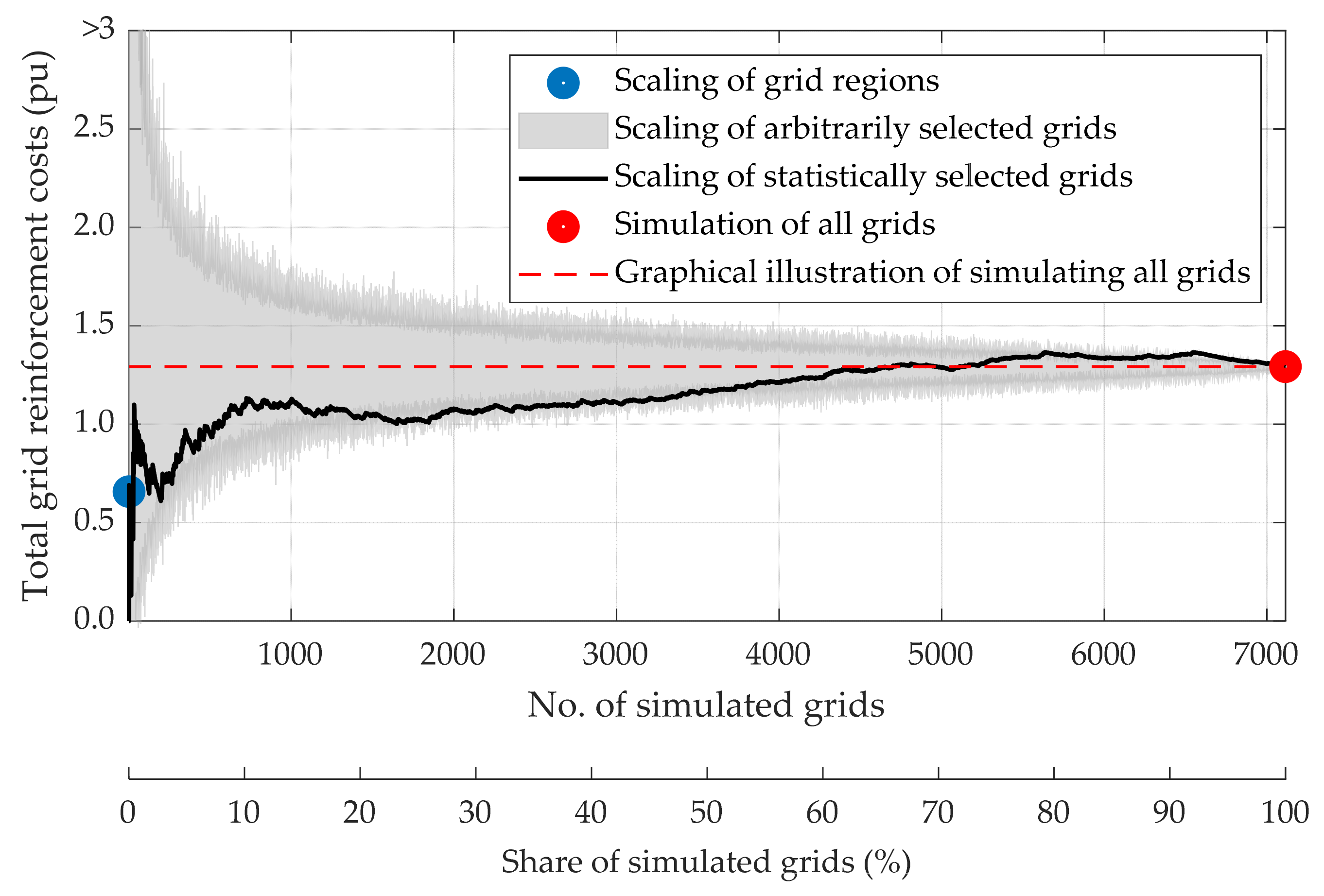
5.1. Comparing Different Quantification Methods

This work analyzes various methods (Table 4) to quantify the total grid reinforcement costs in the selected area, including 7114 LV grids. Due to data protection issues, the actual costs required in the investigated area must not be published. However, the actual costs are divided by a selected non-published reference value to compare various quantification methods. Thus, total grid reinforcement costs determined by the analyzed quantification methods are illustrated as per unit (pu) values depending on the number of simulated grids (Figure 8):
The simulation of one representative grid per grid region (urban, suburban, and rural—three grids in total) and the scaling of their results up to the total number of grids (Scaling of grid regions) reveals total grid reinforcement costs of 0.66 pu. The second method’s results (Scaling of arbitrarily selected grids) strongly depend on the selected grids’ structures. Consequently, this method shows a broad range of possible grid reinforcement costs, especially at a low number of simulated grids. When simulating, for example, 50 randomly chosen grids (0.7% of all grids) and scaling their results to the selected area, the total costs differ between 0.08 pu and 3.18 pu (Figure 8). However, with an increasing number of simulated grids, the spectrum of possible results narrows: Between 0.93–1.68 pu at 1000 simulated grids (14%); between 1.15–1.44 pu at 3500 grids (49%); between 1.23–1.36 pu at 6000 grids (84%).
Total grid reinforcement costs determined by scaling statistically selected grids’ results (method 3) also vary depending on the number of simulated grids. Only 54 of the statistically 500 most representative grids (7.0% of all grids), chosen according to the procedure depicted in Section 4.4, require grid reinforcements in the selected scenario. Scaling their results to the selected area reveals grid reinforcement costs of 1.02 pu. However, the simulation of more grids (and their scaling) leads to total grid reinforcement costs of 1.13 pu (1000 grids), 1.16 pu (3500), and 1.33 pu (6000). Based on the same approach to applying coincidence factors (approach 4: Grid-specific, multiple coincidence factors), quantification methods 2–4 all reveal total costs of 1.29 pu if all 7114 LV grids are simulated (Figure 8).
The results of simulating all LV grids are graphically illustrated in Figure 8 as a red dashed line to provide a better comparison to other quantification methods. The scaling of grid regions’ representative grids (method 1) underestimates grid reinforcement costs by 49% compared to a detailed simulation of all grids (method 4). The scaling of arbitrarily selected and simulated grids (method 2) approaches the actual result (1.29 pu) the more grids are simulated. If LV grids are selected for simulation based on statistical data (method 3), the scaled grid reinforcement costs oscillate around all grids’ aggregated costs (1.29 pu). In this method, all grids are ranked according to their statistical deviation from the “most representative” grid and selected for simulation. The statistically 4600 most representative grids (65%) in the selected area require on average lower grid reinforcement costs (1.7967 × 10⁻⁴ pu) than the overall average of all 7114 grids (1.8165 × 10⁻⁴ pu). Consequently, the scaling of their results underestimates the actual total costs required in the selected area. Simulating between 4601 and 5200 LV grids and scaling their results to the whole area of investigation provides similar (deviation between ±1.6%) results than simulating all grids. However, the simulation and scale of more grids (between 5201 and 7110) overestimate the actual demand of grid reinforcement costs (acquired by simulating all grids). These numbers demonstrate that the “most representative” LV grid in the investigated area shows a high capacity for integrating future customers. On the contrary, total grid reinforcement costs are triggered mainly by grids deviating from the median in the selected area.

5.2. Comparing Different Approaches to Applying Coincidence Factors

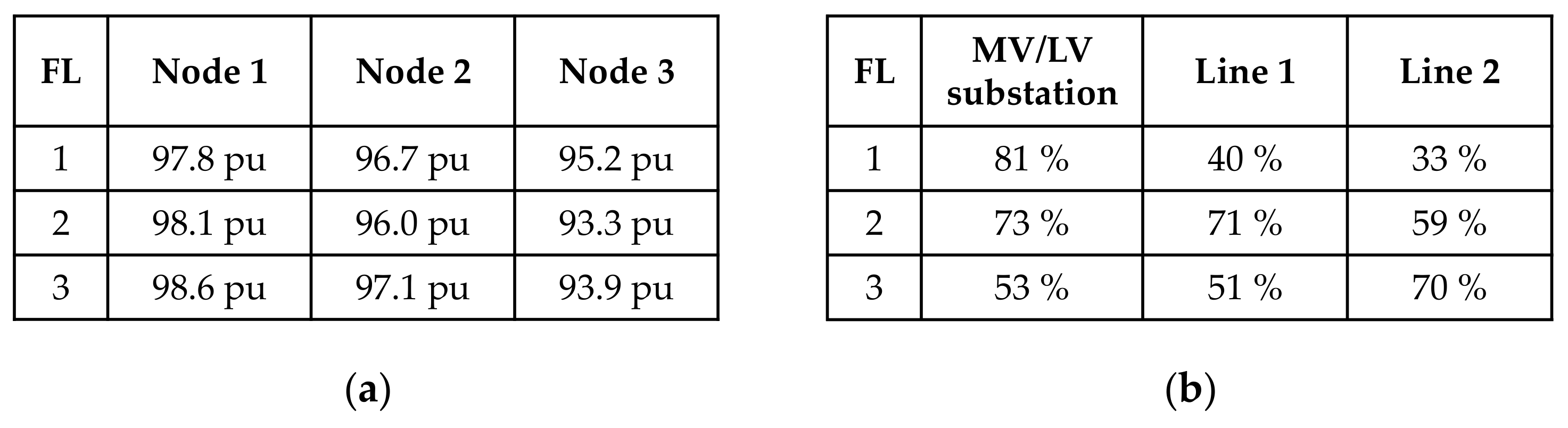
5.2.1. Required Grid Reinforcement Measures

Besides different quantification methods, this study examines various approaches to applying coincidence factors (Table 5) and their suitability for quantifying future grid reinforcement needs. The latter is divided into the total (all 7114 grids) transformer capacity and total length of lines additionally installed to overcome grid restrictions. Similar to costs (Section 5.1), both are divided by selected non-published reference values and illustrated as pu values to fulfill all data protection criteria (Figure 9):
A consistent, single coincidence factor determined based on the average number of customers supplied by the MV/LV substation and applied to each grid (approach 1) neglects the grid’s actual number of customers and misjudges grid conditions in many analyzed grids. As demonstrated in Figure 4, the coincidence factor strongly correlates with the number of customers. Hence, this method overestimates the coincidence factor at the MV/LV substation in grids with considerably more households than the average grid (applied to calculate the coincidence factor in this method). Vice versa, it underestimates the coincidence factor at the MV/LV substation in grids with considerably fewer households. Consequently, the required transformer extensions determined by this method exceed all remaining approaches’ results by 3.22 pu (4.00 pu in total). Since all the other approaches determine grid-specific coincidence factors for the MV/LV substation (feeder level 1), they indicate the same transformer reinforcements, i.e., 0.78 pu (Figure 9). However, the significant discrepancy between consistent and grid-specific coincidence factors (413%) demonstrates the importance of determining the actual coincidence factor at the MV/LV substation for each grid individually. Otherwise, potential grid restrictions are misjudged significantly.
The investigated approaches to applying coincidence factors also differ concerning their resulting line extension needs (Figure 9): Applying single coincidence factors, defined according to the number of customers the MV/LV substation supplies, reveals total line extensions of 0.66 pu (approach 1: Consistent) and 0.24 pu (approach 2: Grid-specific). A value of 0.63 pu is detected, considering grid-specific, double coincidence factors at the MV/LV substation and each feeder’s main line (approach 3, feeder level 1 and 2). Simulating each feeder level, including grid-specific, multiple coincidence factors (approach 4), provides a total line extension of 1.20 pu.
These results demonstrate the importance of applying grid customers’ coincidence factors appropriately: Considering single coincidence factors based on grid elements in feeder level 1 (MV/LV substation) underestimates grid loads at higher feeder levels since coincidence factors rise with lower numbers of customers (Figure 4). Hence, using these methods, the sum of indicated line extension measures in all 7114 LV grids is 45% (approach 1: Consistent) and 80% (approach 2: Grid-specific) lower than the exact consideration of all feeder levels (approach 4). As already mentioned, the consistent coincidence factor of 0.26 (applied in approach 1) overestimates the coincidence factor for many grids’ MV/LV substation (feeder level 1). However, since the coincidence factor increases with an increasing feeder level (decreasing number of grid customers), it estimates grid loads at higher feeder levels and line congestions more appropriately (Figure 9).
Even the application of grid-specific, double coincidence factors (approach 3) according to the MV/LV substation and each feeder’s main line (feeder level 1 and 2) underestimates the total length of additionally required lines (Figure 9): Only 53% of line reinforcement measures are indicated compared to considering grid customers’ coincidence for each grid element in approach 4 (all feeder levels). This discrepancy demonstrates that in the investigated LV grids, a large part of grid reinforcements are required at higher feeder levels, i.e., grid elements distanced from the MV/LV substation.

5.2.2. Required Grid Reinforcement Costs

Similar to Section 5.1, the total grid reinforcement costs, determined using various approaches to applying coincidence factors, are divided by a non-published reference value and illustrated as pu values (Figure 10). This study uses the same cost parameters of transformer- and line reinforcements for each approach (Table 3). However, due to significant differences concerning the required grid reinforcement measures (Figure 9), the examined applications of coincidence factors evaluate total grid reinforcement costs differently. Consistent, single coincidence factors (approach 1) result in total grid reinforcement costs of 1.09 pu (Figure 10). Determining single coincidence factors (MV/LV substation) for each grid individually provides total grid reinforcement costs of 0.33 pu (approach 2). Considering each grid’s coincidence factor at the MV/LV substation and each feeder’s main line and applying both for load flow simulations increases the required costs to 0.72 pu (approach 3). Applying grid-specific, multiple coincidence factors depending on the grid element to be analyzed (approach 4) detects total costs of 1.29 pu, which are needed to prevent potential grid congestions in the analyzed scenario.
The comparison of all approaches reveals the following insights: Applying consistent, single coincidence factors to each grid, the overestimation of required transformer extensions, and the underestimation of required line extensions partly balance each other out (Figure 9). Based on the specific cost parameters selected in this study (Table 3), the underestimation of required line extension measures more decisively affects total grid reinforcement costs. As a result, only 84% (−16%) of the grid reinforcement costs in approach 4 (1.29 pu) are also depicted using this simplified method (Figure 10). Compared to the application of one consistent coincidence factor to each grid (approach 1), grid-specific values (approach 2) misjudge required line extensions more decisively (Figure 9). Due to a more expensive reinforcement of grid lines (compared to transformers), total grid reinforcement costs deviate even more (−74%).
The consideration of grid-specific, double coincidence factors (approach 3), according to the MV/LV substation and at each feeder’s main line, increases the detected costs. However, even this method misjudges total grid reinforcement costs substantially: Compared to grid-specific, multiple coincidence factors (simulating each feeder level), costs are underestimated by 44%.

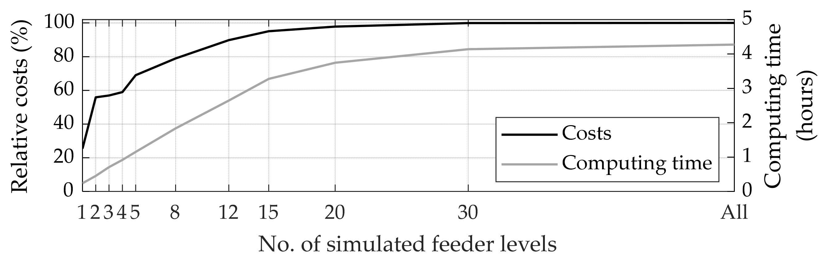
5.2.3. Computing Time

Each approach to applying coincidence factors (Table 5) is tested with the same computing power (32 CPUs, 3 GHz, 128 GB RAM) using the developed large-scale grid simulation tool. However, since they vary in the number of simulated feeder levels, hence, load flow simulations, they show significant differences in the required computing time (Figure 11): Applying single coincidence factors to each grid customer (either consistent or grid-specific) requires one load flow simulation per grid (approaches 1–2). Thus, these methods allow the simulation of all 7114 LV grids in 0.24 h, which corresponds to 1.16 s per 1000 grid nodes (Figure 11).
Two load flow simulations per grid (approach 3), necessary to apply double coincidence factors to grid customers, increase the computing time to 0.45 h for all grids or 2.19 s per 1000 nodes.
Finally, individually considering grid customers’ coincidence factor for each grid element to be analyzed (approach 4) requires 4.27 h in total or 20.77 s per 1000 nodes (Figure 11). The 17.8-times longer computing time, compared to the application of single coincidence factors, correlates with 16.2-times more feeder levels to be simulated on average per grid.

6. Discussion and Outlook

This section discusses the paper’s results (Section 5) and its contribution to the current state of research. Furthermore, it provides an outlook on further work necessary in this field of research. Therefore, this section is divided according to the presented research questions unanswered by the current state of research (Section 3).

6.1. What Is the Potential Error When Simulating Only a Few Individually Selected LV Grids and Scaling Their Results to Quantify Grid Reinforcement Costs in a Large Area?

Present-day LV grids show high discrepancies regarding their maximum hosting capacity considering EVs, PVMs, and HPs [8]. This paper’s results identify the impact of LV grids’ heterogeneity on quantifying future grid reinforcement costs: Considering the analyzed grid area, simulating only a few individually selected grids and scaling their results leads to a broad spectrum of total grid reinforcement costs (Figure 8): If, for example, about 200 grids are selected for load flow simulation (cf. [20,21]), the total costs might deviate between −66% and +82% from the actual value. Assuming actual grid reinforcement costs of 42.5 billion euros [20], this equals a deviation between −28.0 and +34.9 billion euros. Using statistical data to select representative grids (in this work, the root mean square deviation to the median) only slightly decreases the potential error compared to an arbitrary selection of grids to be simulated (Figure 8).
If even fewer grids are simulated, the potential error increases significantly, and the selection of which grids to simulate becomes more crucial. Even if grids are classified depending on their grid region, the simulation of a few grids per region is insufficient to adequately determine overall grid reinforcement costs (Figure 8). However, while this study investigates only one grid per region, selecting other or more grids per region might increase this method’s accuracy. Nevertheless, grid topologies at the LV level significantly fluctuate, even within the same region (urban, suburban, or rural) [48]. Thus, when simulating multiple grids per region, the question of which grids to simulate arises again.

6.2. How Many Grids (in %) Must Be Simulated to Assure a Certain Degree of Accuracy?

The more LV grids are analyzed using load flow simulations, the more accurate future grid reinforcement costs can be estimated (Figure 8). Though, considering the area investigated in this study, up to 5800 grids (82%) must be selected arbitrarily and simulated to enable accuracy of 95%. Decreasing the acceptable accuracy to 85% still requires the simulation of 2800 LV grids (39%).
As demonstrated in Figure 8, selecting representative grids based on statistical data only slightly increases the reliability of results: In some cases, for example, simulating the 4600 (or 5200) most representative grids in the investigated area, total grid reinforcement costs can be determined very accurately (100%). Nevertheless, the acquired results deviate to the same extent as randomly selecting grids. Consequently, the large-scale quantification of potential grid reinforcement costs with adequate accuracy requires simulating several thousand LV grids.

6.3. Impact of the Analyzed Grid’s Variance

It has to be mentioned that this work compares the presented quantification methods only for one Austrian DSO and its LV grids (Section 4.2). Despite similarities to LV grids investigated in other studies (e.g., [49,50,51]), applying the presented insights to other DSOs, hence, different grid topologies and grid planning strategies, requires further investigations. For example, a DSO operating LV grids with similar topology as well as customer density and types may provide deviating results. On this account, we additionally analyze the impact of LV grids’ variance on the share of recommended grids to be simulated. Therefore, similar LV grids are picked from all the LV grids (7114) based on statistical data to establish two classes with different variance: According to Levi et al. [46], Class 1 includes LV grids with a total line length within the 25%-(1.69 km) and 75%-quantile (4.41 km) of all grids. In addition to the total line length, the number of customers per point of common coupling is limited to the 25%-(1.25) and 75%-quantile (2.27) to further decrease the variance of LV grids in class 2. For each class, the share of selected, simulated, and scaled grids is varied between 0–100% (Figure 12).
Decreasing the variance of analyzed LV grids, hence, analyzing more similar grids, allows higher accuracy if simulating only a small share of all grids: Between 0–10% share of simulated grids, the average error is decreased to 13.8% (class 1) and 16.7% (class 2), compared to 32.6% when analyzing all 7114 LV grids (Figure 8). However, despite the lower variance in total line length and customers per point of common coupling, the potential error increases if simulating more grids (>10%): From a maximum error of 23% when analyzing all 7114 grids to 24% (class 1) and 28% (class 2) when analyzing more similar grids (Figure 12).
These results demonstrate that even if the analyzed LV grids show a lower variance, their required reinforcement costs due to future customers might deviate substantially. Consequently, the potential error when simulating representative grids and scaling their results to the whole area of investigation grids must not be neglected.
As illustrated in Figure 12, LV grids vary significantly even within the same class. Hence, the same question arises when classifying grids into representative classes (cf. [5,7,19,20]). Only if grids are classified finely enough, and multiple grids are simulated per class, the scaling of grid reinforcement costs enables adequate accuracy. On the other hand, this approach requires lengthy pre-processing, with huge time- and computation effort [15]. In fact, recent studies using this approach (e.g., [5,20]) analyze all grids of Germany, which justifies time-consuming pre-processing. Since this study investigates one particular service area, including 7114 LV grids, this approach (including pre-processing) would require more time than the simulation of all grids. How to apply grid customers’ coincidence factors to quantify grid reinforcement measures accurately (consistent or grid-specific; single or multiple; based on which grid element)?
Besides the necessity to simulate several thousand grids, this paper’s results (Section 5.2) illustrate another crucial aspect to quantify required grid reinforcements adequately: The appropriate application of grid customers’ coincidence factors. Therefore, this section provides relevant guidelines to accomplish that. While the question of which coincidence factors to use has already been answered in Thormann et al. [8], these guidelines focus on how to apply them for simulating numerous grids:
Firstly, assuming one consistent coincidence factor for each grid (approach 1) is inappropriate to identify grid conditions in several thousand LV grids. This method misjudges both required transformer (overestimated) and line extensions (underestimated) significantly (Figure 9). While in this study, both errors partly balance each other out regarding total grid reinforcement costs (Figure 10), this effect strongly depends on the selected cost parameters. Applying, for example, higher specific transformer costs might increase this method’s error. Thus, each grid’s coincidence factor must be specifically defined depending on its number of supplied customers to overcome this problem.
However, determining single coincidence factors according to the number of customers supplied by the MV/LV substation (approaches 1–2) misjudges grid elements at higher feeder levels, i.e., nodes, transformers, or lines more distanced to the MV/LV substation. The application of double coincidence factors, based on the number of customers supplied by the MV/LV substation and each feeder’s main line (Figure 3), only slightly increases the accuracy of results (approach 3). Consequently, grid customers’ actual coincidence factor must be defined individually for each grid element depending on the number of supplied customers (approach 4). Only then, future grid reinforcement measures and resulting costs can be calculated accurately. As demonstrated in Section 2.3, the current state of research, using coincidence factors [6,7,10,20,23,26], neglects these guidelines. Consequently, their estimated grid reinforcement costs due to future EVs, PVMs, and HPs, might be even higher.
Nevertheless, discrepancies between the analyzed approaches to use coincidence factors apply to the investigated service area with primarily suburban and rural LV grids. Considering grid customers’ coincidence only at the MV/LV substation or each feeder’s main line might be more accurate if applied to urban LV grids, often characterized by fewer grid nodes. Furthermore, due to the selected cost parameters (Table 3), line extensions more significantly affect total grid reinforcement costs than the installation of additional transformers. Cost deviations between the analyzed approaches might be lower, applying higher transformer costs. On this account, the impact of various grid topologies, grid planning strategies, and cost parameters on this issue will be analyzed in further studies.

6.4. What Is the Trade-Off between the Acquired Simulation Accuracy and Required Computing Time?

As demonstrated in Section 4.1.3, the coincidence factor of each grid customer can be considered accurately by simulating multiple feeder levels (Section 4.1.3). While this measure increases the accuracy of grid simulations (Figure 9), it increases the required computing time (Figure 11). However, what is the trade-off between the results’ accuracy and required computing time? In other words: How many feeder levels must be simulated to determine grid reinforcement costs adequately? To answer this question, we vary the number of simulated feeder levels from one (determining single coincidence factors) to all feeder levels (determining multiple coincidence factors, according to the grid element to be analyzed) when simulating all 7114 LV grids. Furthermore, we compare the determined total grid reinforcement costs and the required computing time (Figure 13).
This time, costs are referred to the value of 1.29 pu (Figure 10), acquired by the most accurate application of coincidence factors (simulation of all feeder levels). As demonstrated in Section 5.2, the simulation of one or two feeder levels allows fast computation (0.24 and 0.45 h). Though, it results in lower costs (26% and 56%) than the simulation of all feeder levels. Despite twice the computing time (0.90 h), a further increase to four feeder levels to be simulated only slightly increases accuracy (+3%). This effect is because only a few customers are connected between feeder levels 2 and 4, inhibiting a more accurate consideration of customers’ coincidence. However, at least 95% accuracy requires the simulation of at least 15 feeder levels (Figure 13), which requires 3.3 h of computation. Since not all LV grids are characterized by more than 15 feeder levels, the simulation of all feeder levels only slightly enhances the accuracy of results (+5%). Though, it extends the required computing time by one hour (+23%).

6.5. How to Quantify Future Grid Reinforcement Costs Allowing Both High Accuracy and Adequate Computing Time in the Most Optimal Way?

While Section 5.1 highlights the need for large-scale grid simulations to quantify future grid reinforcement costs, Section 5.2 demonstrates two criteria they should comply with: Applying grid customers’ coincidence factors appropriately depending on the grid element to be analyzed and keeping the required computing time adequate. Both criteria are fulfilled using the developed large-scale grid simulation tool (Section 4.1). The former is tackled by simulating multiple feeder levels and adapting grid customers’ coincidence factors accordingly. Thereby, temporal interdependences between existing (e.g., households) and future customers (EVs, PVMs, and HPs) are accounted for accurately.
Despite the simulation of multiple feeder levels, the required computing time remains reasonable: 20.8 s per 1000 grid nodes. Assuming 104 nodes per grid on average (Section 4.2), about 1600 LV grids can be simulated per hour. In conclusion, the developed tool enables the fast quantification of future grid reinforcement measures and costs with high accuracy. Thereby, it helps to avoid the misjudgment of future power grid investments caused by poor grid selection and inadequate applications of coincidence factors.
Besides classic grid reinforcements (e.g., exchange of transformers or grid lines), grid congestions caused by future customers can be limited or even be prevented by grid-relieving measures. Grid restrictions on the LV level triggered by future EVs can successfully be reduced by demand-side measures, e.g., the adaption of charging power based on appropriate user tariffs [57,58,59,60,61,62]. Furthermore, the conventional power system’s transition towards a power electronics-based power system promotes the provision of grid ancillary services, such as active- or reactive power control. Recent studies [63,64,65,66,67,68] demonstrated these measures’ potential to mitigate grid overloads. Based on their grid-relieving impact, these measures can save investment costs of the DSO by delaying the upgrade of LV infrastructure, such as adding new cables [69,70]. According to Durusut et al. [24], demand-side measures, for example, can reduce the required grid reinforcement costs by 7% in the UK.
However, the potential of grid-relieving measures to mitigate grid restrictions strongly depends on the investigated grid and its region [71]: While urban LV grids are rather characterized by thermal overload, suburban and rural ones are more likely to face voltage violations [8]. Consequently, the quantification of future grid reinforcement costs implementing these measures in a large area will once again require the simulation of numerous grids. Since this paper focuses on comparing different methods to quantify grid reinforcement costs (and not the determined costs themselves), grid-relieving measures are neglected in this work. Nevertheless, the authors will further develop the presented automated large-scale grid simulation tool and implement various flexibility options (e.g., demand-side management, active- and reactive power control, energy storage systems). Thereby, various grid-relieving measures as a countermeasure to classic grid reinforcements can be evaluated considering a large area with several thousand grids.
In addition, the developed large-scale grid simulation tool is restricted in its current version to static deterministic load flow simulations. On the one hand, those provide significant advantages regarding the required computing time when simulating several thousand LV grids. On the other, they inhibit the consideration of time-related effects, crucial to investigate the duration of grid restrictions (e.g., the long-term of thermal overloads) and the potential of flexibility options (e.g., the implementation of energy storages or demand-side measures).
The authors’ following works will further extend the grid simulation tool to allow both fast computation and the consideration of time-related effects: Static deterministic grid simulations are initially performed for several thousand grids to identify potentially endangered grids (based on worst-case conditions). Endangered grids are further examined based on time series-based load flow simulations regarding the duration of grid elements and the potential for implementing grid-relieving measures. Furthermore, the developed tool will be provided as open-source MATLAB code (e.g., GitHub, MATLAB File Exchange) to allow its free application by the scientific community and grid planners.

7. Conclusions

In the analyzed service area operated by an Austrian distribution system operator, low-voltage grids differ significantly in topology and grid customers. As a result, the applied quantification method (scaling of simulated grids’ results or simulating all grids) has a significant influence on quantifying future grid reinforcement costs: The simulation of only a few grids and the scaling of their grid reinforcement costs to the whole service area strongly depends on the selected grids. In case of a poor grid selection, total grid reinforcement costs in the analyzed area might be misjudged significantly using this quantification method. The classification of low-voltage grids in the analyzed area according to their region or grid parameters (e.g., number of customers, total line length) only slightly increases the reliability of results. Consequently, large-scale grid simulations are crucial to quantify grid reinforcement costs triggered by future electric vehicles, photovoltaic modules and electric heat pumps. By varying the approach to applying coincidence factors, this work additionally highlights the importance of accurate grid simulations when quantifying grid reinforcement costs: Simplified approaches, often applied in the current state of research, require only one or two load flow simulations per grid and allow a fast investigation of several thousand grids. Nevertheless, their misjudgment of grid customers’ coincidence factor when evaluating remaining grid elements underestimates required grid reinforcement measures and costs. As a countermeasure, multiple coincidence factors must be applied to grid customers, according to the grid element to be analyzed. While this measure moderately increases the total computing time, it decisively enhances the acquired simulation accuracy.
Knowing the substantial influence of the applied quantification method and the application of coincidence factors helps classify recent studies in this field and their results. Furthermore, the large-scale grid simulation tool developed in this study enables additional analyses by investigating several thousand low-voltage grids with reasonable computing effort. In contrast to recently published grid simulation tools, grid customers’ coincidence factors are accurately considered. Thereby, future grid reinforcement costs due to electric vehicles, photovoltaic modules, or electric heat pumps can accurately be determined while keeping the required computing time adequate.

Author Contributions

Conceptualization, B.T. and T.K.; Data curation, B.T.; Formal analysis, B.T.; Funding acquisition, T.K.; Investigation, B.T.; Methodology, B.T. and T.K.; Project administration, T.K.; Resources, B.T. and T.K.; Software, B.T.; Supervision, T.K.; Validation, B.T. and T.K.; Visualization, B.T.; Writing—original draft, B.T.; Writing—review & editing, T.K. All authors have read and agreed to the published version of the manuscript.

Funding

This research received no external funding.

Conflicts of Interest

The authors declare no conflict of interest.

References

  1. European Commission. Communication from the Commission to the European Parliament, the European Council, the Council, the European Economic and Social Committee and the Committee of the Regions: The European Green Deal; European Commission: Brussels, Belgium, 2019. [Google Scholar]
  2. Austrian Federal Government. Government Program 2020–2024: Out of a Sense of Responsibility for Austria. Available online: https://www.bmoeds.gv.at/Ministerium/Regierungsprogramm.html (accessed on 31 January 2020).
  3. European Parliament; Council. Directive 2010/31/EU of the European Parliament and of the Council of 19 May 2010 on the Energy Performance of Buildings; EUR-Lex: Luxembourg, 2010. [Google Scholar]
  4. Mulenga, E.; Bollen, M.H.; Etherden, N. A review of hosting capacity quantification methods for photovoltaics in low-voltage distribution grids. Int. J. Electr. Power Energy Syst. 2020, 115, 105445. [Google Scholar] [CrossRef]
  5. Büchner, J.; Katzfey, J.; Flörcken, O.; Moser, A.; Schuster, H.; Dierkes, S.; van Leeuwen, T.; Verheggen, L.; Uslar, M.; van Amelsvoort, M. Moderne Verteilnetze fuer Deutschland. Verteilernetzstudie. 2014. Available online: www.bmwi.de/Redaktion/DE/Publikationen/Studien/verteilernetzstudie.html (accessed on 18 August 2021).
  6. Gupta, R.; Pena-Bello, A.; Streicher, K.N.; Roduner, C.; Farhat, Y.; Thöni, D.; Patel, M.K.; Parra, D. Spatial analysis of distribution grid capacity and costs to enable massive deployment of PV, electric mobility and electric heating. Appl. Energy 2021, 287, 116504. [Google Scholar] [CrossRef]
  7. Agora Verkehrswende; Agora Energiewende. Regulatory Assistance Project (RAP). Verteilnetzausbau für die Energiewende–Elektromobilität im Fokus. 2019. Available online: https://www.agora-verkehrswende.de/veroeffentlichungen/studie-verteilnetzausbau-fuer-die-energiewende (accessed on 12 February 2021).
  8. Thormann, B.; Kienberger, T. Evaluation of Grid Capacities for Integrating Future E-Mobility and Heat Pumps into Low-Voltage Grids. Energies 2020, 13, 5083. [Google Scholar] [CrossRef]
  9. Salah, F.; Ilg, J.P.; Flath, C.M.; Basse, H.; van Dinther, C. Impact of electric vehicles on distribution substations: A Swiss case study. Appl. Energy 2015, 137, 88–96. [Google Scholar] [CrossRef]
  10. Association of Austrian Electricity Companies. Netzberechnungen Österreich-Einfluss der Entwicklungen von Elektromobilität und Photovoltaik auf das Österreichische Stromnetz. Available online: www.oesterreichsenergie.at/die-welt-des-stroms/stromnetze/studie-netzberechnungen-oesterreich.html (accessed on 5 January 2021).
  11. Horowitz Kelsey, A.W.; Ding, F.; Mather, B.; Palmintier, B. The Cost of Distribution System Upgrades to Accommodate Increasing Penetrations of Distributed Photovoltaic Systems on Real Feeders in the United States. Available online: www.nrel.gov/docs/fy18osti/70710.pdf (accessed on 3 November 2021).
  12. Li, G.; Zhang, X.-P. Modeling of Plug-in Hybrid Electric Vehicle Charging Demand in Probabilistic Power Flow Calculations. IEEE Trans. Smart Grid 2012, 3, 492–499. [Google Scholar] [CrossRef]
  13. Grainger, J.J.; Stevenson, W.D. Power System Analysis; McGraw-Hill: New York, NY, USA, 1994; ISBN 0-07-113338-0. [Google Scholar]
  14. Werth, T. Netzberechnung mit Erzeugungsprofilen; Springer Fachmedien Wiesbaden: Wiesbaden, Germany, 2016; ISBN 978-3-658-12727-5. [Google Scholar]
  15. Eberl, T.; Hufendiek, K.; Wiest, P.; Rudion, K. Integrale Modellierung von Verteilnetzen und Verteilter Erzeugung. 2014. Available online: www.ieh.uni-stuttgart.de/forschung/forschungsprojekte/integrale-modellierung-von-verteilnetzen-und-verteilter-erzeugung (accessed on 1 April 2021).
  16. Navarro-Espinosa, A.; Mancarella, P. Probabilistic modeling and assessment of the impact of electric heat pumps on low voltage distribution networks. Appl. Energy 2014, 127, 249–266. [Google Scholar] [CrossRef]
  17. Torres, S.; Durán, I.; Marulanda, A.; Pavas, A.; Quirós-Tortós, J. Electric vehicles and power quality in low voltage networks: Real data analysis and modeling. Appl. Energy 2022, 305, 117718. [Google Scholar] [CrossRef]
  18. Tie, C.H.; Gan, C.K.; Ibrahim, K.A. The impact of electric vehicle charging on a residential low voltage distribution network in Malaysia. In Proceedings of the 2014 IEEE Innovative Smart Grid Technologies-Asia (ISGT Asia) Conference, Kuala Lumpur, Malaysia, 20–23 May 2014; IEEE: Piscataway, NJ, USA, 2014; pp. 272–277. [Google Scholar]
  19. Vu, T. A Stochastic Methodology to Determine Reinforcement Cost of Power Distribution Grid for Integrating Increasing Share of Renewable Energies and Electric Vehicles; IEEE: Piscataway, NJ, USA, 2018; pp. 1–5. [Google Scholar] [CrossRef]
  20. Agricola, A.; Höflich, B.; Richard, P.; Völker, J.; Rehtanz, C.; Greve, M.; Gwisdorf, B.; Kays, J.; Noll, T.; Schwippe, J.; et al. Dena-Verteilnetzstudie. Ausbau- und Innovationsbedarf der Stromverteilnetze in Deutschland bis 2030. Energiesysteme und Energiedienstleistungen: Berlin, Germany. 2012. Available online: https://www.dena.de/themen-projekte/projekte/energiesysteme/dena-verteilnetzstudie/ (accessed on 1 April 2021).
  21. Matrose, C.; Helmschrott, T.; Godde, M.; Szczechowicz, E.; Schnettler, A. Impact of different electric vehicle charging strategies onto required distribution grid reinforcement. In Proceedings of the 2012 IEEE Transportation Electrification Conference and Expo. (ITEC), Dearborn, MI, USA, 18–20 June 2012; Staff, I., Ed.; IEEE: Piscataway, NJ, USA, 2012; pp. 1–5. [Google Scholar]
  22. Pudjianto, D.; Djapic, P.; Dragovic, J.; Strbac, G. Grid Integration Cost of Photovoltaic Power Generation. Available online: https://helapco.gr/pdf/PV_PARITY_D44_Grid_integration_cost_of_ (accessed on 14 January 2022).
  23. Hartvigsson, E.; Odenberger, M.; Chen, P.; Nyholm, E. Estimating national and local low-voltage grid capacity for residential solar photovoltaic in Sweden, UK and Germany. Renew. Energy 2021, 171, 915–926. [Google Scholar] [CrossRef]
  24. Durusut, E.; Slater, S.; Strbac, G.; Pudjianto, D.; Djapic, P.; Aunedi, M. Infrastructure in a Low-Carbon Energy System to 2030. Transmission and Distribution: Final Report; Imperial College London: London, UK, 2014. [Google Scholar]
  25. Flinn, J.; Webber, C.; Tong, N.; Cox, R. Customer Distributed Energy Resources Grid Integration Study: Residential Zero Net Energy Building Integration Cost Analysis; California Public Utilities Commission: San Francisco, CA, USA, 2017. [Google Scholar]
  26. Lemmens, J.; Macharis, B.; Gys, R.; Vonken, D. Data-Driven Asset Management with the NGIN Analytics Platform: Assessing EV and PV Impact on the Flemish LV Grid; CIRED: Liège, Belgium, 2019. [Google Scholar]
  27. Rothrock, L.; Narayanan, S. Human-in-the-Loop Simulations; Springer London: London, UK, 2011; ISBN 978-0-85729-882-9. [Google Scholar]
  28. Willis, H.L. Power Distribution Planning Reference Book, 2nd ed.; CRC Press: Boca Raton, FL, USA, 2004; ISBN 0824748751. [Google Scholar]
  29. Resch, M.; Bühler, J.; Klausen, M.; Sumper, A. Impact of operation strategies of large scale battery systems on distribution grid planning in Germany. Renew. Sustain. Energy Rev. 2017, 74, 1042–1063. [Google Scholar] [CrossRef] [Green Version]
  30. Bielecki, S. Estimation of maximum loads of residential electricity users. E3S Web Conf. 2019, 137, 1006. [Google Scholar] [CrossRef]
  31. Wahl, M.; Hein, L.; Moser, A. Fast Power Flow Calculation Method for Grid Expansion Planning. In Proceedings of the 2019 21st European Conference on Power Electronics and Applications (EPE ‘19 ECCE Europe), Genova, Italy, 3–5 September 2019; pp. 1–7. [Google Scholar]
  32. Scheidler, A.; Braun, M.; Kraiczy, M. Automated Grid Planning for Distribution Grids with Increasing PV Penetration. In Proceedings of the 6th Solar Integration Workshop, Vienna, Austria, 14–15 November 2016. [Google Scholar]
  33. Ulffers, J.; Scheidler, A.; Töbermann, J.-C.; Braun, M. Grid Integration Studies for eMobility Scenarios with Comparison of Probabilistic Charging Models to Simultaneity Factors. In Proceedings of the 2nd E-Mobility Power System Integration Symposium, Delft, The Netherlands, 10 October 2018. [Google Scholar]
  34. NEPLAN AG. NEPLAN.; Küsnacht, Switzerland. Available online: https://www.neplan.ch/?lang=de (accessed on 5 February 2022).
  35. DIgSILENT GmbH. PowerFactory. Gomaringen, Germany. Available online: https://www.digsilent.de/de/powerfactory.html (accessed on 3 February 2022).
  36. Fox, B.; Morrow, J.D.; Akmal, M.; Littler, T. Impact of heat pump load on distribution networks. IET Gener. Transm. Distrib. 2014, 8, 2065–2073. [Google Scholar] [CrossRef] [Green Version]
  37. Protopapadaki, C.; Saelens, D. Heat pump and PV impact on residential low-voltage distribution grids as a function of building and district properties. Appl. Energy 2017, 192, 268–281. [Google Scholar] [CrossRef]
  38. Widén, J.; Wäckelgård, E.; Paatero, J.; Lund, P. Impacts of distributed photovoltaics on network voltages: Stochastic simulations of three Swedish low-voltage distribution grids. Electr. Power Syst. Res. 2010, 80, 1562–1571. [Google Scholar] [CrossRef] [Green Version]
  39. Pflugradt, N. Online Load Profile Generator. Available online: https://www.loadprofilegenerator.de (accessed on 8 December 2021).
  40. Heffernan, W.; Watson, N.R.; Buehler, R.; Watson, J.D. Harmonic performance of heat-pumps. J. Eng. 2013, 2013, 31–44. [Google Scholar] [CrossRef]
  41. Kusch, W.; Stadler, I.; Bhandari, R. Heat pumps in low voltage distribution grids by energy storage. In Proceedings of the 2015 International Energy and Sustainability Conference (IESC), Farmingdale, NY, USA, 12–13 November 2015; pp. 1–6. [Google Scholar] [CrossRef]
  42. UNE. Voltage Characteristics of Electricity Supplied by Public Electricity Networks; EN 50160; Beuth: Berlin, Germany, 2011. [Google Scholar]
  43. Laribi, O.; Rudion, K. Optimized Planning of Distribution Grids Considering Grid Expansion, Battery Systems and Dynamic Curtailment. Energies 2021, 14, 5242. [Google Scholar] [CrossRef]
  44. Scheffler, J. Verteilnetze auf dem Weg zum Flächenkraftwerk; Springer: Berlin/Heidelberg, Germany, 2016. [Google Scholar] [CrossRef]
  45. Cloteaux, B. Limits in Modeling Power Grid Topology. In Proceedings of the 2013 IEEE 2nd Network Science Workshop (NSW), West Point, NY, USA, 29 April–1May 2013. [Google Scholar] [CrossRef]
  46. Levi, V.; Strbac, G.; Allan, R. Assessment of performance-driven investment strategies of distribution systems using reference networks. IEE Proc. Gener. Transm. Distrib. 2005, 152, 1. [Google Scholar] [CrossRef]
  47. Traupmann, A.; Kienberger, T. Test Grids for the Integration of RES—A Contribution for the European Context. Energies 2020, 13, 5431. [Google Scholar] [CrossRef]
  48. Postigo Marcos, F.; Mateo Domingo, C.; Gómez San Román, T.; Palmintier, B.; Hodge, B.-M.; Krishnan, V.; de Cuadra García, F.; Mather, B. A Review of Power Distribution Test Feeders in the United States and the Need for Synthetic Representative Networks. Energies 2017, 10, 1896. [Google Scholar] [CrossRef] [Green Version]
  49. Scheffler, J. Bestimmung der Maximal Zulässigen Netzanschlussleistung Photovoltaischen Energiewandlungsanlagen in Wohnsiedlungsgebieten. Ph.D. Thesis, Technischen Universität Chemnitz, Düsseldorf, Germany, 2004. [Google Scholar]
  50. Pagani, G.A.; Aiello, M. Towards Decentralization: A Topological Investigation of the Medium and Low Voltage Grids. IEEE Trans. Smart Grid 2011, 2, 538–547. [Google Scholar] [CrossRef]
  51. Strunz, K.; Fletcher, R.H.; Campbell, R.; Gao, F. Developing benchmark models for low-voltage distribution feeders. In Proceedings of the 2009 IEEE Power & Energy Society General Meeting, Calgary, AB, Canada, 26–30 July 2009; pp. 1–3. [Google Scholar] [CrossRef]
  52. Umweltbundesamt GmbH. Elektromobilität in Österreich: Szenario 2020 und 2050. REP-0257. 2010. Available online: https://www.umweltbundesamt.at/fileadmin/site/publikationen/REP0257.pdf (accessed on 18 July 2021).
  53. Fechner, H. Ermittlung des Flächenpotentials für den Photovoltaik-Ausbau in Österreich: Welche Flächenkategorien sind für die Erschließung von Besonderer Bedeutung, um das Ökostromziel Realisieren zu Können, Vienna. 2020. Available online: https://oesterreichsenergie.at/downloads/publikationsdatenbank/detailseite/photovoltaik-ausbau-in-oesterreich (accessed on 25 December 2021).
  54. Fraunhofer IWES/IBP. Wärmewende 2030: Schlüsseltechnologien zur Erreichung der Mittel- und Langfristigen Klimaschutzziele im Gebäudesektor. Available online: https://www.agora-energiewende.de/fileadmin/Projekte/2016/Sektoruebergreifende_EW/Waermewende-2030_WEB.pdf (accessed on 30 July 2021).
  55. European Commision. Degree of Urbanisation (DEGURBA)-Local Administrative Units. Available online: https://ec.europa.eu/eurostat/ramon/miscellaneous/index.cfm?TargetUrl=DSP_DEGURBA (accessed on 26 June 2020).
  56. Kadam, S. Defintion and Validation of Reference Feeders for Low-Voltage Networks. Ph.D. Thesis, Technical University Wien, Vienna, Austria. Available online: https://repositum.tuwien.at/handle/20.500.12708/7709 (accessed on 18 August 2021).
  57. Shao, S.; Pipattanasomporn, M.; Rahman, S. Demand Response as a Load Shaping Tool in an Intelligent Grid with Electric Vehicles. IEEE Trans. Smart Grid 2011, 2, 624–631. [Google Scholar] [CrossRef]
  58. Faddel, S.; Mohammed, O.A. Automated Distributed Electric Vehicle Controller for Residential Demand Side Management. IEEE Trans. Ind. Appl. 2019, 55, 16–25. [Google Scholar] [CrossRef]
  59. Brinkel, N.; Schram, W.L.; AlSkaif, T.A.; Lampropoulos, I.; van Sark, W. Should we reinforce the grid? Cost and emission optimization of electric vehicle charging under different transformer limits. Appl. Energy 2020, 276, 115285. [Google Scholar] [CrossRef]
  60. Richardson, P.; Flynn, D.; Keane, A. Local Versus Centralized Charging Strategies for Electric Vehicles in Low Voltage Distribution Systems. IEEE Trans. Smart Grid 2012, 3, 1020–1028. [Google Scholar] [CrossRef]
  61. Clement-Nyns, K.; Haesen, E.; Driesen, J. The Impact of Charging Plug-In Hybrid Electric Vehicles on a Residential Distribution Grid. IEEE Trans. Power Syst. 2010, 25, 371–380. [Google Scholar] [CrossRef] [Green Version]
  62. García-Villalobos, J.; Zamora, I.; Knezović, K.; Marinelli, M. Multi-objective optimization control of plug-in electric vehicles in low voltage distribution networks. Appl. Energy 2016, 180, 155–168. [Google Scholar] [CrossRef] [Green Version]
  63. Geth, F.; Leemput, N.; van Roy, J.; Buscher, J.; Ponnette, R.; Driesen, J. Voltage droop charging of electric vehicles in a residential distribution feeder. In Proceedings of the 2012 3rd IEEE PES Innovative Smart Grid Technologies Europe (ISGT Europe 2012), International Conference and Exhibition, Berlin, Germany, 14–17 October 2012; IEEE: Piscataway, NJ, USA, 2012; pp. 1–8. [Google Scholar]
  64. Ireshika, M.A.S.T.; Lliuyacc-Blas, R.; Kepplinger, P. Voltage-Based Droop Control of Electric Vehicles in Distribution Grids under Different Charging Power Levels. Energies 2021, 14, 3905. [Google Scholar] [CrossRef]
  65. Al-Awami, A.T.; Sortomme, E.; Asim Akhtar, G.M.; Faddel, S. A Voltage-Based Controller for an Electric-Vehicle Charger. IEEE Trans. Veh. Technol. 2016, 65, 4185–4196. [Google Scholar] [CrossRef]
  66. Zecchino, A.; Marinelli, M. Analytical assessment of voltage support via reactive power from new electric vehicles supply equipment in radial distribution grids with voltage-dependent loads. Int. J. Electr. Power Energy Syst. 2018, 97, 17–27. [Google Scholar] [CrossRef]
  67. Knezović, K.; Marinelli, M. Phase-wise enhanced voltage support from electric vehicles in a Danish low-voltage distribution grid. Electr. Power Syst. Res. 2016, 140, 274–283. [Google Scholar] [CrossRef] [Green Version]
  68. Thormann, B.; Braunstein, R.; Wisiak, J.; Strempfl, F.; Kienberger, T. Evaluation of grid relieving measures for integrating electric vehicles in a suburban low-voltage grid. In CIRED Conference Proceedings 2019; CIRED: Liège, Belgium, 2019. [Google Scholar]
  69. UK Power Networks. Network Impacts of Supply-Following Demand Response: Report A6. Available online: https://innovation.ukpowernetworks.co.uk (accessed on 8 February 2022).
  70. Aigner, M.; Schmautzer, E.; Friedl, B.; Bliem, M.; Haber, A. Synergetic effects for DSOs and customers caused by the integration of renewables into the distribution network-Influences on business and national economics. In CIRED Conference Proceedings 2015; CIRED: Liège, Belgium, 2015. [Google Scholar]
  71. Turton, H.; Moura, F. Vehicle-to-grid systems for sustainable development: An integrated energy analysis. Technol. Forecast. Soc. Chang. 2008, 75, 1091–1108. [Google Scholar] [CrossRef]
Figure 1. Typical grid topology of one low-voltage (LV) feeder supplying four grid customers.
Energies 15 01383 g001
Figure 2. Scheme of the developed fully automated large-scale grid simulation tool.
Energies 15 01383 g002
Figure 3. Structuring the grid topology into feeder levels.
Energies 15 01383 g003
Figure 4. Novel coincidence factors considering temporal interdependences between various customer types: households, electric vehicles (EVs), photovoltaic modules (PVMs), and heat pumps (HPs).
Energies 15 01383 g004
Figure 5. Exemplary allocation of coincidence factors (CF) and resulting power (P) to the grid’s customers depending on the analyzed feeder level (FL).
Energies 15 01383 g005
Figure 6. Exemplary output of static load flow simulations performed for three feeder levels (FL): Each node’s voltage (a) and the thermal utilization of the MV/LV substation and lines (b).
Energies 15 01383 g006
Figure 7. Frequency of occurrence of (a) the installed transformer capacity, (b) the number of nodes, (c) the total line length, and (d) the number of customers per point of common coupling (PCC) in the analyzed LV grids.
Energies 15 01383 g007
Figure 8. Comparison of different quantification methods regarding their detected total grid reinforcement costs depending on their number and share of simulated grids.
Energies 15 01383 g008
Figure 9. Comparison of different approaches to applying coincidence factors (CF) regarding the required transformer- and line extensions (7114 LV grids simulated).
Energies 15 01383 g009
Figure 10. Comparison of different approaches to applying coincidence factors (CF) regarding the required grid reinforcement costs (7114 LV grids simulated).
Energies 15 01383 g010
Figure 11. Comparison of different approaches to applying coincidence factors (CF) regarding the required computing time (7114 LV grids simulated).
Energies 15 01383 g011
Figure 12. Comparison of scaling statistically selected LV grids’ results for two grid classes, classified according to the total line length and the number of customers per point of common coupling (PCC).
Energies 15 01383 g012
Figure 13. Grid reinforcement costs (relative to the simulation of all feeder levels) and required computing time depending on the number of simulated feeder levels.
Energies 15 01383 g013
Table 1. Classification of recent studies according to their method to quantify total grid reinforcement costs for several thousand grids.
Method to Quantify Total Grid Reinforcement CostsStudies
Simulation of representative grid structures and scaling of their results:[5,7,10,19,20,21,22,23,24,25]
- synthetic grids modeled based on real-life grid data[5,19,22,23,24]
- real-life grids selected from the area of investigation[7,10,20,21,25]
- classification of grids into representative classes[5,7,19,20]
Large-scale grid simulation of numerous real-life grid models[6,10,26]
Table 2. Classification of recent studies according to their approach to modeling grid customers’ load.
Applied Approach to Modeling Grid Customers’ LoadStudies
No specification[24]
Time series-based simulation[22]
Monte-Carlo simulation[5,19,21]
Deterministic grid simulations using coincidence factors:[6,7,10,20,23,25,26]
- single, consistent coincidence factor[20,25]
- single, grid-specific coincidence factor[6,23,26]
- double, grid-specific coincidence factors[7,10]
Table 3. Parameters applied for determining required grid reinforcement costs [7,20,44].
ParameterApplied Values
Max. number of parallel transformers (-)2
Max. number of parallel lines (-)4
Nominal power of additional transformers (MVA)0.1, 0.25, 0.4, 0.63, 0.8, 1.0, 1.25
Material and installation costs of additional transformers (k€)7.0, 17.3, 27.7, 29.6, 35.6, 38.0, 41.4
Specific construction costs of additional grid lines (€/km)65,000
Specific material costs of additional grid lines (€/km)10,000
Table 4. Evaluated methods to quantify future grid reinforcement costs.
Quantification MethodSelection of Representative Grids to Be SimulatedNo. of Simulated Grids
1Scaling of grid regionsBased on the grid planner’s
expertise (one per region)
3
2Scaling of arbitrarily
selected grids
Randomly for 1000 iterationsVaried between
1–7114
3Scaling of statistically
selected grids
Based on statistical dataVaried between
1–7114
4Simulation of all grids-7114
Table 5. Evaluated approaches to applying coincidence factors (CF).
CF-Variation in the Analyzed Grids No. of Various CFs Applied per GridGrid Element as Basis of CF-DeterminationSimulated Feeder Levels
1ConsistentSingleMV/LV substationFeeder level 1
2Grid-specificSingleMV/LV substationFeeder level 1
3Grid-specificDoubleMV/LV substation and each feeder’s main lineFeeder level 1
and 2
4Grid-specificMultipleEach grid elementAll feeder levels
Publisher’s Note: MDPI stays neutral with regard to jurisdictional claims in published maps and institutional affiliations.

