
Surrogate DC Microgrid Models for Optimization of Charging Electric Vehicles under Partial Observability


1
Faculty of Electrical Engineering, Mathematics and Computer Sciences, Delft University of Technology, Van Mourik Broekmanweg 6, 2628 XE Delft, The Netherlands
2
DC Opportunities R&D B.V., Molengraaffsingel 12, 2629 JD Delft, The Netherlands
*
Author to whom correspondence should be addressed.
Energies 2022, 15(4), 1389; https://0-doi-org.brum.beds.ac.uk/10.3390/en15041389
Submission received: 19 December 2021
/
Revised: 19 January 2022
/
Accepted: 9 February 2022
/
Published: 14 February 2022
(This article belongs to the Special Issue Control and Optimization in a DC Microgrid)
Abstract
:Many electric vehicles (EVs) are using today’s distribution grids, and their flexibility can be highly beneficial for the grid operators. This flexibility can be best exploited by DC power networks, as they allow charging and discharging without extra power electronics and transformation losses. From the grid control perspective, algorithms for planning EV charging are necessary. This paper studies the problem of EV charging planning under limited grid capacity and extends it to the partially observable case. We demonstrate how limited information about the EV locations in a grid may disrupt the operation planning in DC grids with tight constraints. We introduce two methods to change the grid topology such that partial observability of the EV locations is resolved. The suggested models are evaluated on the IEEE 16 bus system and multiple randomly generated grids with varying capacities. The experiments show that these methods efficiently solve the partially observable EV charging planning problem and offer a trade-off between computational time and performance.
1. Introduction
The increasing penetration of electric vehicles (EVs) and renewable energy sources (RES) into distribution grids provides new opportunities, but also poses new challenges for the system operators. As EVs and some of the RES inherently use DC, they can be integrated into DC grids without additional converters and with smaller power losses [1]. For this reason, DC in distribution grids is considered to be a suitable alternative to the currently used AC [2]. Unlike conventional loads, EVs are flexible in terms of when their demand should be served. This flexibility is provided by a special entity, the EV aggregator [3], which coordinates the charging of EVs. The goal of the aggregator is to solve the EV charging planning (EVCP) problem, i.e., to minimize the sum of unmet demand and operation costs, while not violating the physical constraints of the grid.
In practice, there are two main challenges related to solving the EVCP problem. First, information about the EV parameters (e.g., arrival and departure times, demand and locations in the grid) and/or the grid state (topology, physical properties of the nodes or lines) may not be fully available to the EV aggregator. Hence, the aggregator might have to operate using incomplete information. Second, as the relation between current and voltage is hyperbolic, the power flow equation makes the EVCP problem non-convex [4]. That means not only that there is no theoretical guarantee of obtaining the globally optimal solution, but also that the problem may become computationally intractable for large grids and long planning horizons.
A popular perspective on the EVCP problem is to simplify or even omit the power flow equations and grid constraints, in order to make the problem tractable. Various studies have pursued this approach and focused on dealing with the uncertainty of the future EV arrivals. Sadeghianpourhamami et al. [5] applied a reinforcement learning algorithm to coordinate the EV charging in a constraint-free grid. In [6], the authors minimized the problem’s Lagrangian in a decentralized fashion to optimize the charging of the EVs located in a single building with stochastic wind power supply. Wu and Sioshansi [7] designed a two-stage optimization algorithm with a sample-average approximation technique to solve the EVCP problem using a linearization of the AC power flow. On the other hand, some studies have combined the EVCP with the non-convex optimal power flow (OPF) problem and included the exact power flow equations and grid constraints in it. Kayacık et al. [8] formulated the EVCP problem as a multi-timestep OPF problem extended with additional constraints on the CO2 emissions and derived a convex second-order cone programming relaxation that can be solved efficiently. In [9], a fuzzy-logic controller was developed to minimize power costs and emissions simultaneously. Chen et al. [10] solved the EVCP+OPF problem by decoupling the OPF part from the planning and using the convex dual problem for it. However, no studies have included both incomplete information or EV uncertainties and power flow equations in the EVCP problem.
While the uncertainty of the EV parameters and non-convexity of the OPF are usually considered separately in the existing literature, in reality the EV aggregator should solve both problems simultaneously. The direct combination of the existing solutions for these problems does not seem possible: two-stage optimization of a non-convex problem easily becomes intractable. On the other hand, model-free methods, such as reinforcement learning, are generally hard to apply to constraint optimization problems. Moreover, if the present, rather than the future, is not fully known (e.g., due to privacy concerns), the standard EVCP formulation becomes irrelevant, and further research is required to formulate and solve the partially observable version of the problem.
An important input group of parameters for the EVCP problem is the locations of the EVs in the grid, as they are necessary to compute the power flow required for charging. This study investigates the EVCP with partial observability of the EV locations. The problem is reformulated to account for partial observability, and we investigate how it affects the EV aggregator by answering the following questions:
- How crucial is it for the EV aggregator to know exact locations of the EVs in the grid?
- How can one obtain a well-performing, scalable solution when the EV locations are known only up to certain degree?
In order to answer the first question, we conducted experiments on DC grids with various topologies and capacities to evaluate how different degrees of awareness about EV locations affect the planning. The experimental results demonstrate that a lack of information about the locations of the EVs currently present in the grid considerably disrupts the performance, whereas locations of the EVs that are yet to arrive are much less vital. To deal with this issue, this paper introduces two alternatives for modeling the grid topology without knowing the exact locations of the EVs. Experiments on both real and randomly generated grids show that the suggested models perform better than a naive baseline and offer a trade-off between computational cost and performance.
2. Background
2.1. EVCP Problem Formulation
Existing studies consider various formulations of the EVCP problem depending on the optimization objective, EV charging approach, and optimization approach [3]. This study adopts the perspective of an EV aggregator that represents the combined interest of all the EVs in a grid. Its goal is to maximize the social welfare—the sum of the demand provided to the EVs—with minimal operation costs. Following [10,11], EV charging optimization is combined with power flow equations and grid constraints. Unlike most existing studies, this work does not assume that all vehicles can be charged fully. To account for that, all EVs have a linear utility function quantifying how much value each car assigns to being charged for one Watt Hour.
Advances in power electronics allow for new solutions in the microgrid design. Various aspects of DC microgrids’ control, protection, and energy management are being studied in the literature (e.g., see [12] for an overview). As this paper aims at solving the charging planning problem with partial observability, we employ the relatively simple DC microgrid model suggested in [13]. For the same reason, this work does not consider the properties of the EV batteries, as they does not affect the charging planning algorithm. This study considers DC microgrids that consist of multiple EV charging stations and one or several generators that can represent connections to an external power grid or distributed generators (DGs). Prior to defining the optimization problem for the EVCP in DC grids, we introduce the necessary notation.
The set of nodes in the grid (the squared cup symbol ⊔ is the disjoint union operator) is a disjoint union of the loads and generators For convenience, we use n and m as subscripts when we mean an arbitrary node and use subscripts l and g to highlight the difference between the loads and generators. The set of lines contains the node pairs that are connected by a line. The set is the set of planning timesteps, each timestep having a constant length, being defined as At each timestep voltage and power in the loads l and generators g are denoted by and correspondingly. Line current and conductance between nodes n and m are denoted by and , respectively. For each generator , we define energy supply costs as a linear function of the generator’s power with coefficient . We use a convention that power at the generators is negative and power at the loads is positive. The bounds for the voltages, power, and currents are denoted by The set of the electric vehicles is denoted by and each EV has several parameters. Let be the arrival and departure times, be the desired state-of-charge (SOC) at departure, and be the coefficient of the linear utility function specifying the priority of the particular EV. SOC at timestep t is denoted by For simplicity, we use to denote the load where EV k is being charged and for the EV at load
First, the power flow constraints are defined as follows:
Then, the EV state-of-charge is subject to the following constraints:
The optimization objective of the EVCP problem is defined as
We call J the social welfare as it combines the fulfilled demand weighted by the EV utility coefficients and the negative of the operation costs. The coefficients can represent the generation costs or price for buying power from the external grid. The utility coefficients are defined per EV and represent the importance of each vehicle. It is worth mentioning that it is possible to define the utility coefficients per load rather than per EV. In that case, it can be used to model the pricing tariff in the grid. However, the problem will not change mathematically, and hence we do not deliberately study this case. The constraints (1a–e) and (2a–c) and the objective (3) define the EVCP problem:
2.2. SOCP Relaxation
Due to the Equation (1e), the OPF problem and hence the EVCP problem are non-convex. Several methods to convexify the OPF problem are suggested in the literature, including semi-definite programming (SDP) [4] and second-order convex programming (SOCP) [13] formulations. As the latter has been shown to perform optimally in multiple real DC grids [13], we adapt it to the EVCP problem. The SOCP relaxation can be obtained by the following change of variables:
The constraints (1a–e) can be relaxed to the following quadratic cone constraints:
Then, the SOCP relaxation of the EVCP problem is the following optimization problem:
2.3. Including Uncertainties
If the full information about the EVs and the grid is available to the EV aggregator, then the only challenge for solving the exact EVCP problem is its non-convexity. As discussed in the previous section, convex relaxation techniques such as SDP or SOCP are demonstrated to be effective solutions for that. In practice, however, the information that the aggregator has access to might be limited. For example, due to causality, parameters of an EV usually become known only after it arrives in the grid, hence making the EVCP a stochastic optimization problem. Moreover, if RES [6] or inelastic loads [10] are included in the problem, their generation and demand are usually also modeled as random variables. A common approach to solving the EVCP problem with uncertainties is online planning, where the problem is repeatedly solved at each timestep.
An important feature of online planning is that it allows one to obtain a feasible solution of the EVCP problem even in the presence of future uncertainties. However, a conceptually different example emerges when the state of the grid is only partially observable. For example, changes in the grid topology, variations in nodal and line limits, or locations of the EVs in the grid might be reported to the aggregator with a delay. In this case, the EVCP problem cannot be formulated in the standard way, because its constraints are unknown. Furthermore, as the solution is not guaranteed to be feasible, the objective value cannot be used to evaluate the solution’s quality. The next section presents a way to define the EVCP problem with partial observability and introduce an evaluation framework that can be used with it.
3. Partially Observable EVCP
In a partially observable EVCP (PO-EVCP) problem, the EV aggregator may be unaware of some input parameters of the EVCP problem. This study considers the case when the locations of the EVs in the grid are only partially known. Specifically, the loads in a distribution grid are divided in several regions, which are referred to in this paper as cables. For example, the cables can correspond to charging stations at different streets or EV parking lots. Then, the EV aggregator only knows at which cables EVs are parked. In practice, that can be relevant due to the privacy concerns or limited communication between the EV aggregator and the grid operator.
First, let be the set of cables, where a single cable contains several loads Every load in the grid belongs to one cable, i.e., For simplicity, the cable corresponding to load l is denoted by The EV aggregator only knows the cable where an EV is parked, but the particular load is a random variable. Its distribution can be obtained by the following process: initially, all loads in the grid are unoccupied. Then, for each timestep if an EV k arrives in the grid, its location is sampled uniformly from the unoccupied nodes in the cable The sampled load becomes occupied until the EV departs.
In the PO-EVCP problem, the feasibility region defined by (1a–e) and (2a–c) is stochastic. The remainder of this section introduces three approximate approaches to resolving the partial observability of the problem.
3.1. Blind Guessing Model
The simplest way to derive a deterministic approximation for the PO-EVCP problem is to sample the positions of incoming EV uniformly from the unoccupied loads. Note that the sampled and the actual positions will rarely coincide. Let and be vectors of the loads and EVs, respectively, and let be the true unknown assignment of grid loads to EVs. Blind guessing is defined as this random sampling of an assignment , and we denote the resulting EV-to-load and load-to-EV maps as and , respectively. In the EVCP problem, only constraint (2c) and objective (3) depend on Hence, they can be rewritten as follows:
Then, the PO-EVCP problem with blind guessing can be defined:
Essentially, the blind guessing model resolves the uncertainty in the PO-EVCP problem by randomly assuming where EVs are parked within the corresponding cable. Then, the problem is reduced to the standard exact EVCP problem, defined in Section 2.1.
3.2. Surrogate Grid Models
As an alternative to blindly guessing the EV assignments, it is possible to instead modify the grid topology used in the optimization problem. The goal is to derive a surrogate grid with such topology that the optimization problem becomes independent of the non-observable information. In other words, such surrogate grid should be invariant over different EV assignments, as it effectively makes the problem deterministic. This section presents two different surrogate grid models with this property. Before defining these models, some additional notation is introduced. For each pair of nodes let
denote a path from m to n. The path conductance is defined by the equation
Then, let be the path from m to n with the highest conductance. The conductance of this path is denoted by and its current limit by
The conductance between a cable and an external node is defined as the average conductance over the paths from m to loads in
The current limit between c and m is defined as
Parallel nodes model. The parallel nodes model transforms each cable c into a set of nodes connected in parallel. To derive the parallel nodes surrogate grid, all lines that connect nodes within c are removed. For each connection from an external node to a new node is added and connected to m with and Then, node is connected to all loads in the cable with new lines, such that and The new node is passive; i.e., The parallel nodes’ surrogate grid is illustrated in Figure 1.
Let and be the sets of nodes and lines in the parallel nodes surrogate grid. Then, the optimization problem for the parallel nodes models is the same as the exact EVCP problem with
It is crucial that, due to the topology of the parallel nodes surrogate grid, the optimization problem is equivalent for all values of and hence the partial observability is resolved.
Single node model. The single node model transforms each cable c into a single node For each neighbouring node such that a line is added. Its parameters are defined as and The power bounds for are defined as the sum over original nodes: Voltage bounds are defined as the average: The parallel nodes’ surrogate grid is illustrated in Figure 2.
In the single node surrogate model, all nodes from a cable c are mapped to new node Hence, there are multiple EVs charging at Prior to defining the optimization problem, new notation is introduced. Let be the power provided to EV k at timestep Then, there are the following constraints on and EVs’ SOC.
Let and be the sets of nodes and lines in the single node surrogate grid. Then, the optimization problem for the single node model is defined as follows:
Since all EVs belonging to a cable c in the original problem are charged at the same node in the single node model, the value of the true assignment does not affect the problem. Hence, the partial observability is resolved.
3.3. Planning and Execution
As the PO-EVCP problem with blind guessing or a surrogate grid has a feasibility region different from the one defined by the constraints (1a–e) and (2a–c), it can be impossible to execute its solution. Moreover, though Li et al. [13] demonstrate that SOCP relaxation is exact in various real grids, the theoretical guarantees of the exactness are limited in the presence of line current constraints. Therefore, the solution obtained by solving the PO-EVCP problem using the SOCP relaxation cannot be safely executed in the grid. To account for that, this paper proposes a planning and execution framework that divides the solution process into two consecutive steps. Planning is the process performed by the EV aggregator, aimed at computing the optimal charging schedule under partial observability. Its counterpart, the executor, can be seen as a part of the grid itself. It is a control algorithm responsible for maintaining the grid state within its physical limits. The executor is considered to be fully-aware of the grid state. In this study, the executor is solving a single-timestep OPF problem, since it is one of the most common grid control algorithms and can be implemented in hardware [14].
At each timestep the planner solves an SOCP relaxation of the PO-EVCP problem (using blind guessing or a surrogate grid model). As discussed above, the obtained solution might be imperfect due to the inexactness of the relaxation and/or partial observability. To account for that, planner and executor work in an online fashion: at each timestep the planner solves the PO-EVCP problem and the executor runs the solution. Let be the set of the EVs active at the timestep i.e., Furthermore, let denote the part of the planner’s solution corresponding to the power at timestep t at loads where the EVs from are parked. Then, is used as an input to the executor’s OPF problem:
If is feasible in terms of (1a–e) and the objective is monotonically increasing (which is true if ), the executor problem solution will match The interaction between the planner and the execution is described by Algorithm 1.
| Algorithm 1: Planning and execution framework. |
|
Initialize total social welfare Initialize EVs’ SOC for for do For active EVs obtain by solving the planner problem Create the executor problem using Solve the executor problem, obtain power at loads and objective value for do end for end for |
The planning and execution framework guarantees that each grid state is always feasible, and hence allows for evaluation of inexact planners, such as the surrogate grid and blind guessing planners.
4. Experiments
We simulated the EVCP problem using the planning and execution framework with different planners in order to answer the two following questions:
- How important is the knowledge of the precise EV locations in different DC grids for the EV aggregator to solve the EVCP problem?
- Which approach should the EV aggregator use when EV locations are known only at the cable level?
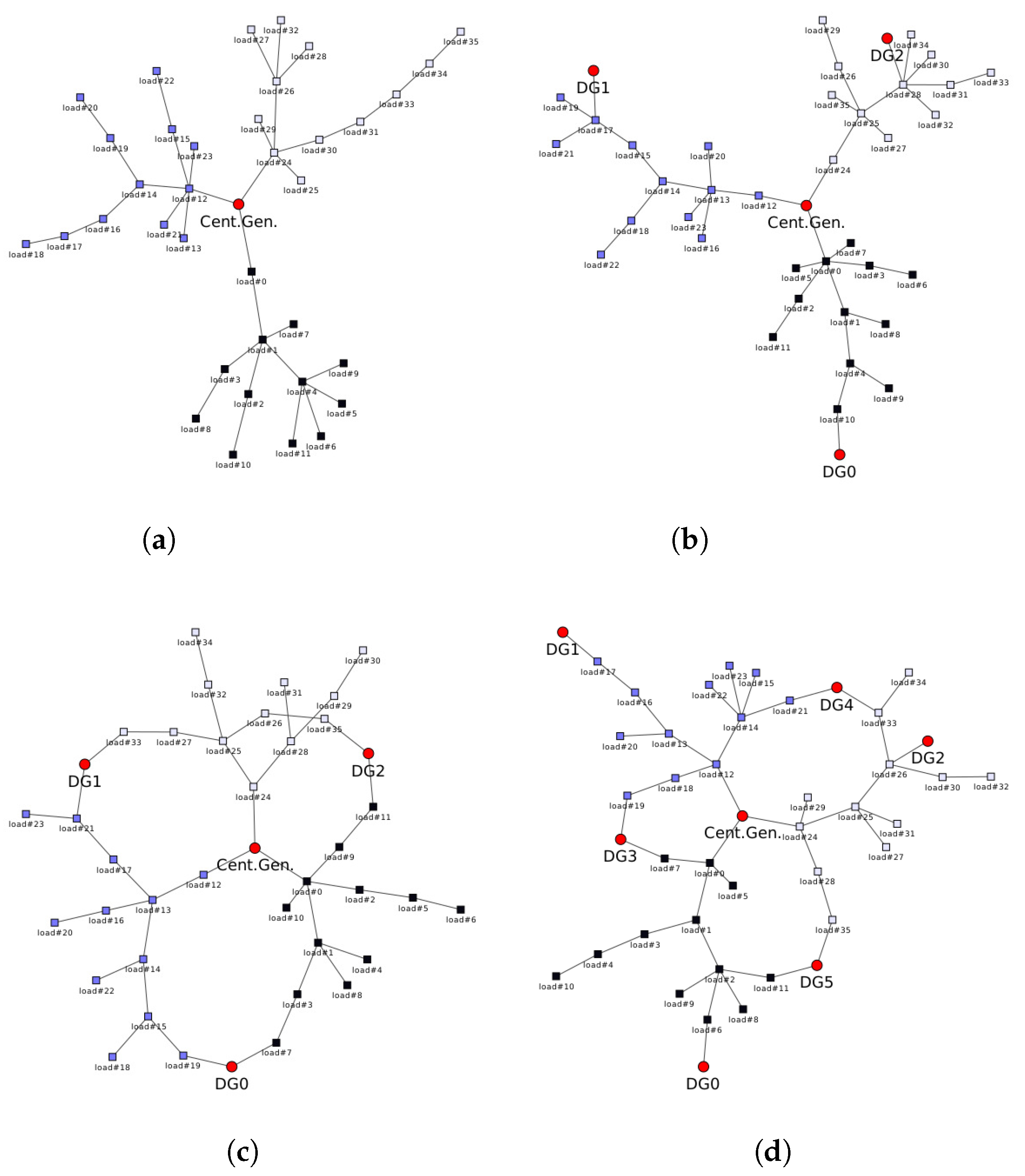
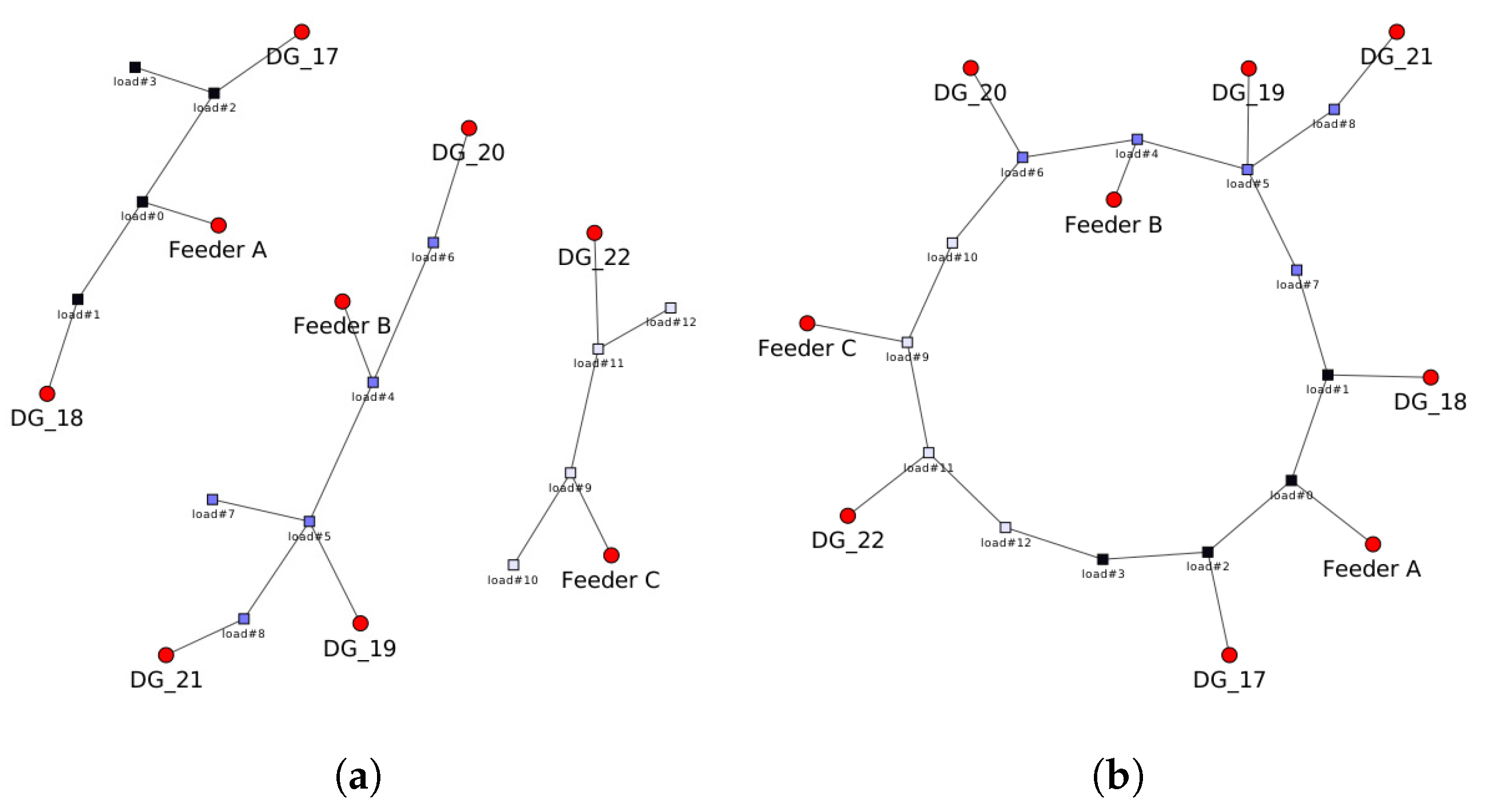
This section describes the details of the simulations and presents the results. Two main components of each simulation are the grid configuration and the scenario. The grid is defined by the numbers of loads, generators, and lines between them; the voltage and power limits of the nodes; and the current limits and conductance of lines. In the experiments, the grid topology was either sampled from the random topology classes (Figure 3) or taken from the real IEEE16 grid [13] (Figure 4). For both meshed and radial topologies of the IEEE16 grid, we considered two cases: with and without connection to the external grid. In the former case, capacities of the feeders A, B, and C were infinite In the disconnected case, the feeder capacities were set to zero For all nodes, the voltage limits were defined as = 300 V, = 400 V. The load power bounds were set to = 10,000 W. The generators power upper bound was set to zero = 0 W (meaning generators cannot consume power), and the lower bound varied across the experiments. The line current limits also varied. The conductance was equal for all lines in all grids, = 15 S. We always set all generators to have the same capacity and cost coefficient The line capacities were also equal for all lines. In the experiments with random grids, we sampled one random topology per value of and
Each scenario contained a power price and EV parameters. The power price for each scenario was sampled from the day-ahead price data for the Netherlands [15]. Figure 5a shows an example of the power price curve for a single day. To sample the EV arrival times, we simulated a non-homogeneous Poisson process independently in each load. The arrival rate was similar across the loads and scenarios and derived from the dataset of EV charging sessions in Dundee, Scotland [16]. Figure 5b demonstrates the dynamics of the EV arrival rate.
The demand, parking time, and utility coefficient were sampled from the normal distributions described in Table 1. It is worth mentioning that we chose values for the utility coefficients such that they were at least an order of magnitude larger than the power price In this case, the objectives in the executor and planner problems were monotonically increasing, i.e., charging an EV always increases the social welfare.
The planning horizon was set to 24 h for all simulations, and timestep size to 30 min. For each grid topology and parameters, we used 6 scenarios to evaluate the performance of the planners.
The optimization routine was performed by MOSEK Fusion API for Python 9.3.10 [17] on a single machine with Intel® Core i7-10700K Processor. We used default solver parameters except for setting basisRelTolS, basisTolS, and intpntCoTolDfeas to The initial conditions and convergence criteria were also default for MOSEK.
4.1. Importance of the Locations
To estimate the importance of knowing the precise EV locations, we tested a blind guessing SOCP planner on the PO-EVCP problem using different degrees of observability of the EV locations (Table 2). The planners were obtaining the assignments by first fixing the precisely known locations and then randomly sampling the remaining locations within the corresponding cables.
We evaluated all four planners by sampling random meshed grids (Figure 3c) with 12 nodes and 4 generators and varying generation capacity and the lines’ current limit Figure 6 demonstrates the provided social welfare as a function of and For better comparability between different topologies, the social welfare is normalized relative to the full planner.
The simulations imply that knowing EV locations becomes important when the line current constraints are tight. On the contrary, the tighter the generation constraints are, less effect is caused by the partial observability. Moreover, the planner with access to the present, but not the future, EV locations (labelled SOCP_present) performed almost optimally, while past and blind planners (SOCP_past and SOCP_blind, respectively) provided considerably less social welfare. Practically, that means that knowing locations of the EVs arriving in the future is not crucial and knowing currently present EVs locations is enough for the EV aggregator to compute the charging schedule. However, when the locations are unavailable even for the active EVs in the grid, the EV aggregator might want to use surrogate grid models for planning.
4.2. Surrogate Grid Models
As demonstrated in the previous section, the blind planner performs suboptimally for tight line constraints. In this section we compare single node and parallel nodes models with the blind planner and demonstrate their benefits for the EV aggregator.
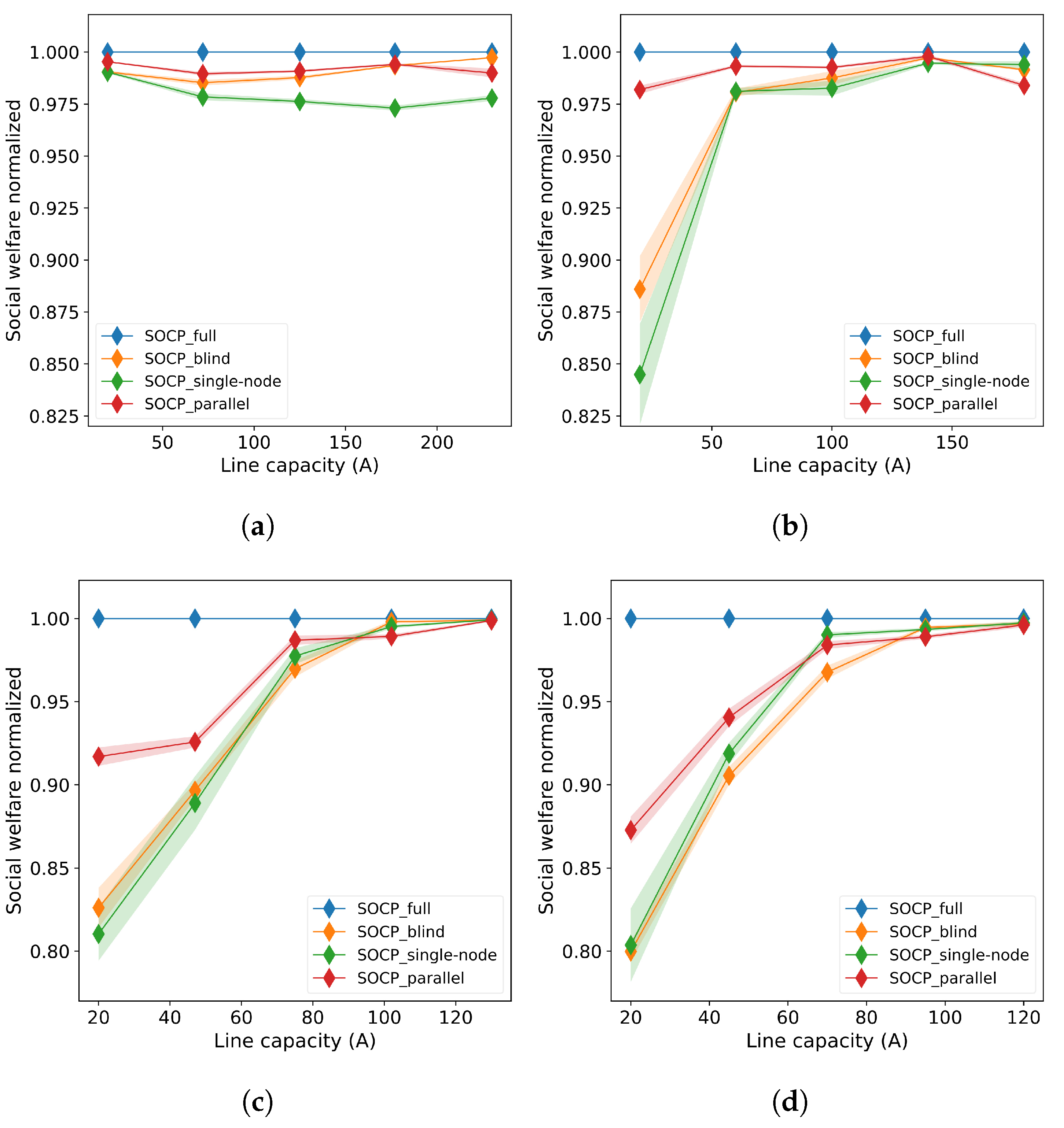
We used all four random topologies from Figure 3 and two versions of the IEEE 16 buses grid (Figure 4) for the simulations. We varied to determine how the tightness of the line constraints affects planing. Importantly, we used different ranges for in different grids, such that the highest value in each range represents the case when the line constraints in the full planner’s solution were not binding. The results for random grids and IEEE16 grids are presented in Figure 7 and Figure 8, respectively. Appendix A also shows the solutions achieved by different planners at one planning timestep.
The results in Figure 7 suggest that all three planners reach nearly optimal performances as the line current constraints become irrelevant. In the tight constraints case, however, the parallel nodes planner (labeled SOCP_parallel) is clearly dominant. The single node (SOCP_single) performs slightly worse than the blind planner in the radial grids, but the gap decreases when the number of generators increases. In the meshed grids with additional DGs, the single node planner outperforms the blind guessing planner.
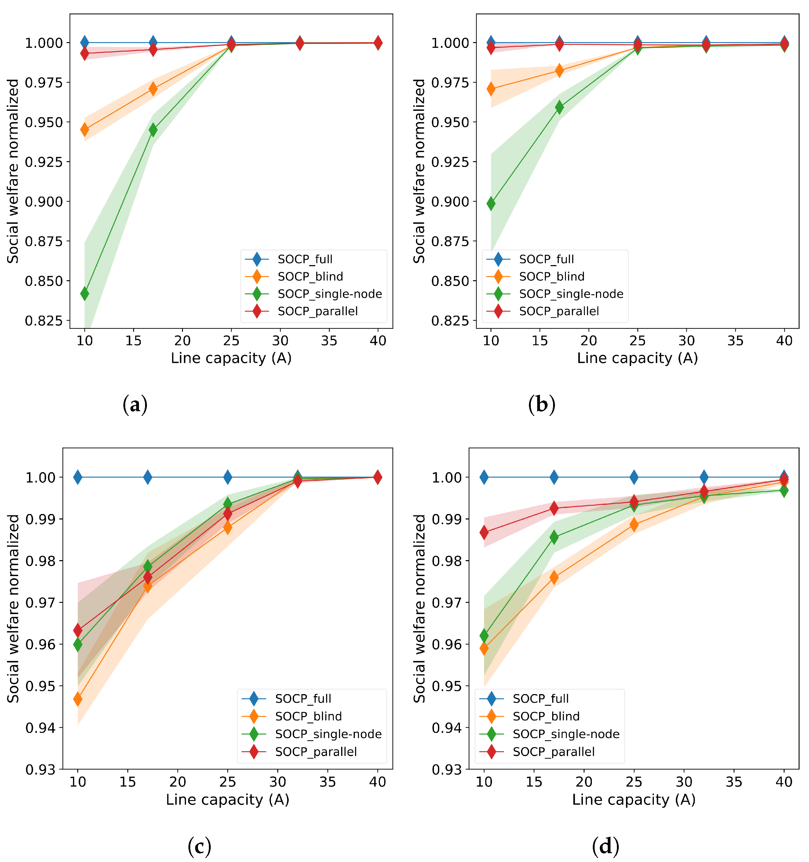
The results in Figure 8 demonstrate similar behavior. Interestingly, the parallel nodes planner is much more dominant in the radial version of the grid. In the meshed case, when more generators are connected to each cable, the single node model again slightly outperforms the blind planner.
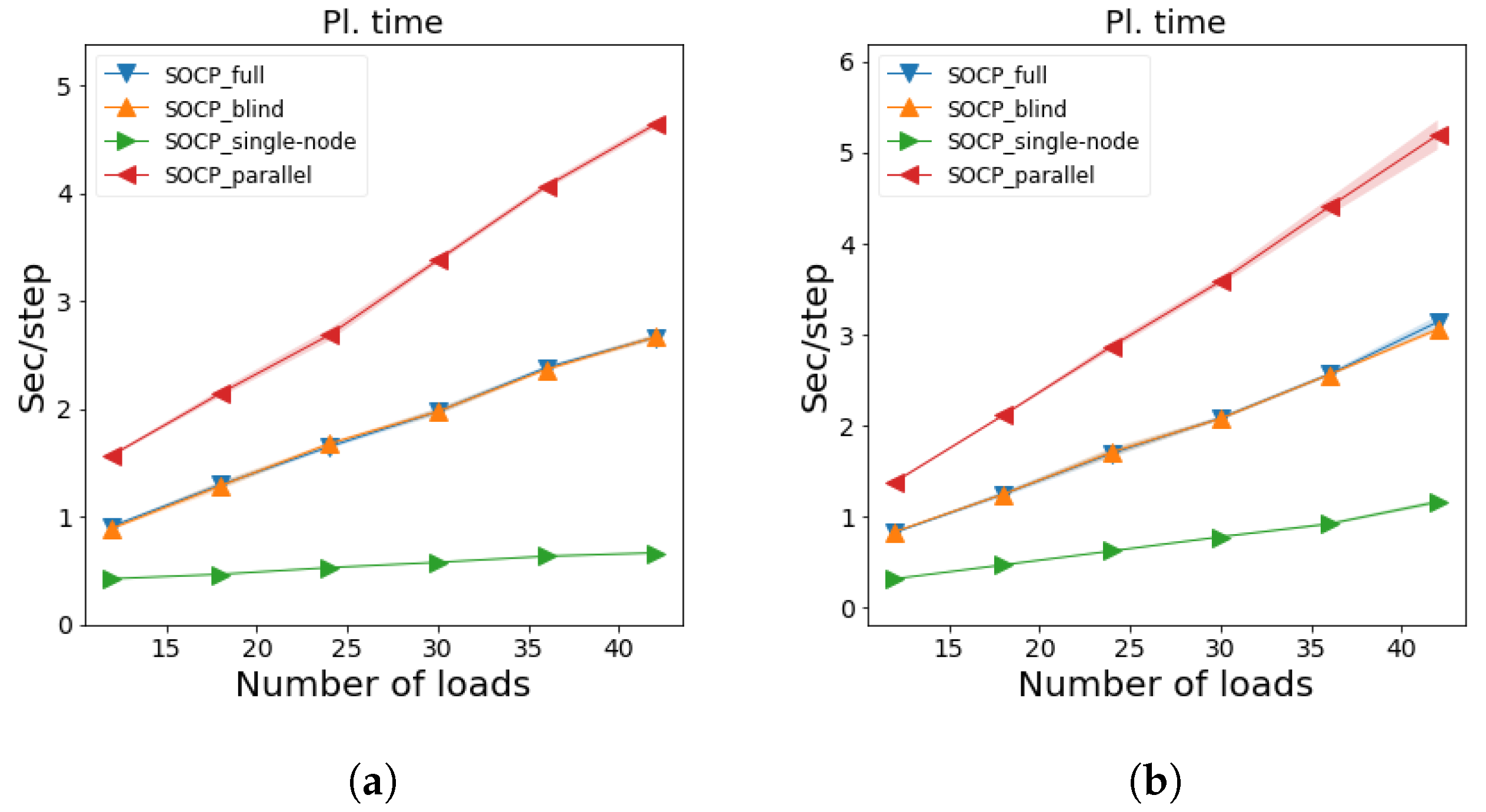
Based on Figure 7 and Figure 8, we may conclude that the parallel nodes planner seems to be the best choice for tightly constrained grids in terms of performance. In practice, however, the computational time may also be an important factor for the EV aggregator. Larger grids and longer planning horizons may make the EVCP problem hardly tractable even using the SOCP relaxation. Since the parallel nodes’ surrogate grid uses more lines and passive nodes than the original grid, it is expected to be the slowest method. Similarly, the single node model should scale best. Figure 9 compares the planning time of different planners as a function of the grid size. For that experiment, we used random radial grids with DGs from Figure 3b. We investigated the planning time in the grids with three cables of varying cable lengths (Figure 9a) and in the grids with varying numbers of cables with six loads (Figure 9b).
The results in Figure 9 confirm the poor scalability of the parallel nodes planner and show the superiority of the single node solution.
5. Conclusions
In this paper, we have extended the EVCP problem for DC microgrids by including partial observability of the EV locations (PO-EVCP). We have studied the effects of partial observability on the performance of planners and suggested two solutions tailored to deal with the unknown EV locations. The experiments in this study lead to the following conclusions about the PO-EVCP:
- 1.
- In DC grids with tight line constraints, knowing the locations of the active EVs in the grid is important for computing charging schedules which maximize the social welfare. Practically, this should be considered when designing a communication protocol between EV owners and the EV aggregator.
- 2.
- If, due to the limitations of the communication scheme or privacy concerns, the EV aggregator can only partially observe the EV locations, it may prefer to use parallel nodes or single node models. The former model is clearly dominant performance-wise, but requires more resources, and the latter offers great scalability at the cost of a tiny performance drop.
To ensure realistic conditions, the experiments in this work included a wide range of line capacities and demands, and also randomly generated topologies. Therefore, we are confident that the conclusions drawn from these simulation results are quite general and will also hold in practice.
Author Contributions
Conceptualization, G.V., W.B., L.M. and M.d.W.; methodology, G.V.; software, G.V.; supervision, W.B., L.M. and M.d.W.; visualization, G.V.; writing—original draft, G.V.; writing—review and editing, G.V., W.B. and M.d.W. All authors have read and agreed to the published version of the manuscript.
Funding
This work was executed with a Topsector Energy Grant from the Ministry of Economic affairs of the The Netherlands.
Data Availability Statement
The code to reproduce the results presented in this study is released and can be accessed at [18].
Conflicts of Interest
The authors declare no conflict of interest.
Abbreviations
The following abbreviations are used in this manuscript:
| EV | Electric vehicle |
| RES | Renewable energy source |
| DC | Direct current |
| AC | Alternating current |
| DG | Distributed generator |
Appendix A. A Solution Example
This appendix demonstrates an example solution for the PO-EVCP problem obtained by different planners. This example was taken from the IEEE16 meshed grid connected to the external grid (Figure 4b). The generation capacitiy in the feeders was unlimited, and set to −144,444 W for the distributed generators. The line current limit, was equal for all lines and set to 17 A. Table A1 and Table A2 demonstrate the solutions obtained by different planners at a single timestep during the simulation.

Table A1.
One timestep of the simulation of the IEEE16 meshed grid with exernal grid connection. Comparison of the exact (fully-observable) and blind planners. Columns voltage (V) and p (W) correspond to the nodal voltage and power obtained by the executor; planned p (W) is the solution derived by the corresponding planner.
| Exact | Blind | |||||
|---|---|---|---|---|---|---|
| Voltage (V) | P (W) | Planned P (W) | Voltage (V) | P (W) | Planned P (W) | |
| Feeder A | 400.0 | −7000.0 | −7000.0 | 399.09 | −6984.0 | −7000.0 |
| Feeder B | 399.94 | −6999.0 | −6999.0 | 400.0 | −7000.0 | −6998.0 |
| Feeder C | 400.0 | −7000.0 | −7000.0 | 399.65 | −6994.0 | −7000.0 |
| load_4 | 398.83 | 6626.0 | 6626.0 | 397.92 | 6965.0 | 6965.0 |
| load_5 | 398.83 | 6962.0 | 6962.0 | 398.42 | 19.0 | 19.0 |
| load_6 | 398.77 | 3756.0 | 3756.0 | 397.43 | 5374.0 | 5374.0 |
| load_7 | 398.18 | 526.0 | 526.0 | 396.67 | 4995.0 | 4995.0 |
| load_8 | 398.77 | 3753.0 | 3753.0 | 398.83 | 30.0 | 30.0 |
| load_9 | 398.83 | 6610.0 | 6610.0 | 398.15 | 6215.0 | 6215.0 |
| load_10 | 398.18 | 7495.0 | 7495.0 | 398.36 | 6980.0 | 6980.0 |
| load_11 | 398.83 | 35.0 | 35.0 | 397.75 | 6325.0 | 6325.0 |
| load_12 | 398.83 | 6980.0 | 6980.0 | 397.73 | 9450.0 | 9450.0 |
| load_13 | 398.83 | 0.0 | 0.0 | 398.48 | 0.0 | 0.0 |
| load_14 | 397.67 | 10,000.0 | 10,000.0 | 397.88 | 6403.0 | 6403.0 |
| load_15 | 398.83 | 0.0 | 0.0 | 397.91 | 0.0 | 0.0 |
| load_16 | 397.67 | 10,000.0 | 10,000.0 | 396.74 | 6483.0 | 10,000.0 |
| DG_17 | 399.94 | −6999.0 | −6999.0 | 398.59 | −6975.0 | −6995.0 |
| DG_18 | 400.0 | −7000.0 | −7000.0 | 399.59 | −6993.0 | −7000.0 |
| DG_19 | 400.0 | −7000.0 | −7000.0 | 399.32 | −6988.0 | −7000.0 |
| DG_20 | 399.34 | −6989.0 | −6989.0 | 399.52 | −6992.0 | −6994.0 |
| DG_21 | 400.0 | −7000.0 | −7000.0 | 398.9 | −6981.0 | −7000.0 |
Table A2.
One timestep of the simulation of the IEEE16 meshed grid with exernal grid connection. Comparison of the single-node and parallel nodes planners. Columns voltage (V) and p (W) correspond to the nodal voltage and power obtained by the executor; planned p (W) is the solution derived by the corresponding planner.
| Single-Node | Parallel Nodes | |||||
|---|---|---|---|---|---|---|
| Voltage (V) | P (W) | Planned P (W) | Voltage (V) | P (W) | Planned P (W) | |
| Feeder A | 398.76 | −6978.0 | −6996.0 | 397.28 | −6952.0 | −6993.0 |
| Feeder B | 398.91 | −6981.0 | −6995.0 | 398.81 | −6979.0 | −6994.0 |
| Feeder C | 400.0 | −7000.0 | −7000.0 | 400.0 | −7000.0 | −6999.0 |
| load_4 | 397.59 | 2788.0 | 2788.0 | 396.11 | 7121.0 | 7121.0 |
| load_5 | 397.06 | 8250.0 | 8250.0 | 396.11 | 7133.0 | 7133.0 |
| load_6 | 397.42 | 4835.0 | 4835.0 | 396.15 | 5866.0 | 5866.0 |
| load_7 | 396.9 | 4997.0 | 4997.0 | 396.0 | 7788.0 | 8292.0 |
| load_8 | 397.74 | 7661.0 | 7661.0 | 397.65 | 5536.0 | 5536.0 |
| load_9 | 397.39 | 6457.0 | 6457.0 | 397.13 | 5537.0 | 5537.0 |
| load_10 | 398.21 | 3669.0 | 3669.0 | 397.92 | 6742.0 | 6742.0 |
| load_11 | 396.75 | 5708.0 | 5708.0 | 396.14 | 5711.0 | 5711.0 |
| load_12 | 397.61 | 5680.0 | 5680.0 | 397.37 | 5533.0 | 5533.0 |
| load_13 | 398.83 | 0.0 | 0.0 | 398.83 | 0.0 | 0.0 |
| load_14 | 398.12 | 4768.0 | 4768.0 | 398.17 | 2552.0 | 2552.0 |
| load_15 | 398.38 | 0.0 | 0.0 | 398.33 | 0.0 | 0.0 |
| load_16 | 397.21 | 5071.0 | 7824.0 | 397.17 | 0.0 | 2844.0 |
| DG_17 | 398.59 | −6975.0 | −6996.0 | 397.31 | −6953.0 | −6993.0 |
| DG_18 | 398.22 | −6969.0 | −7000.0 | 397.27 | −6952.0 | −7000.0 |
| DG_19 | 398.56 | −6975.0 | −6992.0 | 398.3 | −6970.0 | −6993.0 |
| DG_20 | 399.37 | −6989.0 | −7000.0 | 399.09 | −6984.0 | −7000.0 |
| DG_21 | 398.77 | −6979.0 | −6999.0 | 398.54 | −6974.0 | −6995.0 |
References
- Mackay, L.; van der Blij, N.H.; Ramirez-Elizondo, L.; Bauer, P. Toward the Universal DC Distribution System. Electr. Power Compon. Syst. 2017, 45, 1032–1042. [Google Scholar] [CrossRef] [Green Version]
- Al-Ismail, F.S. DC Microgrid Planning, Operation, and Control: A Comprehensive Review. IEEE Access 2021, 9, 36154–36172. [Google Scholar] [CrossRef]
- Amjad, M.; Ahmad, A.; Rehmani, M.H.; Umer, T. A review of EVs charging: From the perspective of energy optimization, optimization approaches, and charging techniques. Transp. Res. Part D Transp. Environ. 2018, 62, 386–417. [Google Scholar] [CrossRef]
- Lavaei, J.; Low, S.H. Zero Duality Gap in Optimal Power Flow Problem. IEEE Trans. Power Syst. 2012, 27, 92–107. [Google Scholar] [CrossRef] [Green Version]
- Sadeghianpourhamami, N.; Deleu, J.; Develder, C. Definition and evaluation of model-free coordination of electrical vehicle charging with reinforcement learning. IEEE Trans. Smart Grid 2018, 11, 203–214. [Google Scholar] [CrossRef] [Green Version]
- Yang, Y.; Jia, Q.S.; Guan, X.; Zhang, X.; Qiu, Z.; Deconinck, G. Decentralized EV-Based Charging Optimization With Building Integrated Wind Energy. IEEE Trans. Autom. Sci. Eng. 2019, 16, 1002–1017. [Google Scholar] [CrossRef]
- Wu, F.; Sioshansi, R. A two-stage stochastic optimization model for scheduling electric vehicle charging loads to relieve distribution-system constraints. Transp. Res. Part B Methodol. 2017, 102, 55–82. [Google Scholar] [CrossRef]
- Kayacık, S.E.; Kocuk, B.; Yüksel, T. The Promise of EV-Aware Multi-Period OPF Problem: Cost and Emission Benefits. arXiv 2021, arXiv:2107.03868. [Google Scholar]
- Azizipanah-Abarghooee, R.; Terzija, V.; Golestaneh, F.; Roosta, A. Multiobjective Dynamic Optimal Power Flow Considering Fuzzy-Based Smart Utilization of Mobile Electric Vehicles. IEEE Trans. Ind. Inform. 2016, 12, 503–514. [Google Scholar] [CrossRef]
- Chen, N.; Quek, T.Q.; Tan, C.W. Optimal charging of electric vehicles in smart grid: Characterization and valley-filling algorithms. In Proceedings of the 2012 IEEE Third International Conference on Smart Grid Communications (SmartGridComm), Tainan, Taiwan, 5–8 November 2012; pp. 13–18. [Google Scholar] [CrossRef] [Green Version]
- Shi, Y.; Tuan, H.D.; Savkin, A.V.; Duong, T.Q.; Poor, H.V. Model Predictive Control for Smart Grids With Multiple Electric-Vehicle Charging Stations. IEEE Trans. Smart Grid 2019, 10, 2127–2136. [Google Scholar] [CrossRef]
- Kaur, S.; Kaur, T.; Khanna, R.; Singh, P. A state of the art of DC microgrids for electric vehicle charging. In Proceedings of the 4th IEEE International Conference on Signal Processing, Computing and Control, ISPCC 2017, Solan, India, 21–23 September 2017; pp. 381–386. [Google Scholar] [CrossRef]
- Li, J.; Liu, F.; Wang, Z.; Low, S.H.; Mei, S. Optimal Power Flow in Stand-Alone DC Microgrids. IEEE Trans. Power Syst. 2018, 33, 5496–5506. [Google Scholar] [CrossRef] [Green Version]
- Palaniappan, R.; Molodchyk, O.; Rehtanz, C. Hardware implementation of an optimal power flow algorithm in a distribution network with decentralised measurements. In Proceedings of the CIRED 2020 Berlin Workshop (CIRED 2020), Online, 22–23 September 2020; Volume 2020, pp. 580–583. [Google Scholar] [CrossRef]
- ENTSO-E Transparency Platform. Available online: https://transparency.entsoe.eu/dashboard/show (accessed on 1 September 2021).
- Electric Vehicle Charging Sessions Dundee. Available online: https://data.dundeecity.gov.uk/dataset/ev-charging-data (accessed on 1 September 2021).
- MOSEK ApS. MOSEK Fusion API for Python 9.3.11. 2021. Available online: https://docs.mosek.com/latest/pythonfusion/index.html (accessed on 1 December 2021).
- Veviurko, G. Software accompanying the publication: Surrogate DC Microgrid Models for Optimization of Charging Electric Vehicles under Partial Observability, 4TU.ResearchData, 2022. [CrossRef]
Figure 1.
An example of the parallel nodes surrogate grid. Rectangular nodes are loads, and red circle nodes are generators. Line capacity is denoted by y and current limit by .
Figure 1.
An example of the parallel nodes surrogate grid. Rectangular nodes are loads, and red circle nodes are generators. Line capacity is denoted by y and current limit by .

Figure 2.
An example of a single node surrogate grid. Rectangular nodes are loads and red circle nodes are generators. Line capacity is denoted by y and current limit by .
Figure 2.
An example of a single node surrogate grid. Rectangular nodes are loads and red circle nodes are generators. Line capacity is denoted by y and current limit by .

Figure 3.
Random grid topologies. Rectangular nodes are loads, red circles are generators. Colors of the loads encode the cables they belong to. (a) Radial grid with single generator. (b) Radial grid with DGs. (c) Meshed grid with DGs between cables. (d) Meshed grid with DGs between and at cables.
Figure 3.
Random grid topologies. Rectangular nodes are loads, red circles are generators. Colors of the loads encode the cables they belong to. (a) Radial grid with single generator. (b) Radial grid with DGs. (c) Meshed grid with DGs between cables. (d) Meshed grid with DGs between and at cables.

Figure 4.
IEEE16 grid from [13]. Rectangular nodes are loads, red circles are generators. Colors of the loads encode the cables they belong to. (a) Radial version. (b) Meshed version.
Figure 4.
IEEE16 grid from [13]. Rectangular nodes are loads, red circles are generators. Colors of the loads encode the cables they belong to. (a) Radial version. (b) Meshed version.

Figure 5.
(a) An example of the power price curve for a single day. (b) Poisson process rate used to model the EV arrivals.
Figure 5.
(a) An example of the power price curve for a single day. (b) Poisson process rate used to model the EV arrivals.

Figure 6.
Results of random guessing planners with different degree of knowledge of the EV locations. Values are normalized relative to the full planner. Horizontal axis is the lines current limit. (a) Normalized social welfare over varying lines current limit, per-generator capacity is fixed at 72 kW. (b) Normalized social welfare over varying single generator’s capacity, per-line current limit is fixed at 56 A.

Figure 7.
Social welfare provided the surrogate models, full and blind planners. Values are normalized relative to the full planner. Horizontal axis is the lines current limit. (a) Radial grid with single generator. (b) Radial grid with DGs. (c) Meshed grid with DGs between cables. (d) Meshed grid with DGs between and at cables.

Figure 8.
Social welfare provided by the surrogate models, full and blind planners. Values are normalized relative to the full planner. Horizontal axis is the lines’ current limit. (a) Radial IEEE16 grid connected to the external grid. (b) Disconnected radial IEEE16 grid. (c) Meshed IEEE16 grid connected to the external grid. (d) Disconnected meshed IEEE16 grid.

Figure 9.
Planning time per timestep for different grid sizes. (a) Random radial grid with DGs with 3 cables each of equal length varying from 4 to 14 (b) Random radial grid with DGs with cables of length 6. The amount of cables varied from 2 to 7.
Figure 9.
Planning time per timestep for different grid sizes. (a) Random radial grid with DGs with 3 cables each of equal length varying from 4 to 14 (b) Random radial grid with DGs with cables of length 6. The amount of cables varied from 2 to 7.

Table 1.
Distributions of the EV parameters.
| Distribution | Unit | |
|---|---|---|
| Desired SOC | Watt | |
| Charging time | Hour | |
| Utility coefficient | $/Watt |
Table 2.
Four degrees of observability of the EV locations.
| Observability | Precisely Known Locations | Locations Known up to Cable |
|---|---|---|
| Full | All EVs | None |
| Present | EVs that have already arrived | EVs arriving in the future |
| Past | EVs that stayed in the grid for at least one timestep | EVs that have just arrived and future EVs |
| Blind | None | All EVs |
Publisher’s Note: MDPI stays neutral with regard to jurisdictional claims in published maps and institutional affiliations. |
© 2022 by the authors. Licensee MDPI, Basel, Switzerland. This article is an open access article distributed under the terms and conditions of the Creative Commons Attribution (CC BY) license (https://creativecommons.org/licenses/by/4.0/).
Share and Cite
MDPI and ACS Style
Veviurko, G.; Böhmer, W.; Mackay, L.; de Weerdt, M. Surrogate DC Microgrid Models for Optimization of Charging Electric Vehicles under Partial Observability. Energies 2022, 15, 1389. https://0-doi-org.brum.beds.ac.uk/10.3390/en15041389
AMA Style
Veviurko G, Böhmer W, Mackay L, de Weerdt M. Surrogate DC Microgrid Models for Optimization of Charging Electric Vehicles under Partial Observability. Energies. 2022; 15(4):1389. https://0-doi-org.brum.beds.ac.uk/10.3390/en15041389
Chicago/Turabian StyleVeviurko, Grigorii, Wendelin Böhmer, Laurens Mackay, and Mathijs de Weerdt. 2022. "Surrogate DC Microgrid Models for Optimization of Charging Electric Vehicles under Partial Observability" Energies 15, no. 4: 1389. https://0-doi-org.brum.beds.ac.uk/10.3390/en15041389
Note that from the first issue of 2016, this journal uses article numbers instead of page numbers. See further details here.