A Comparative Study and Optimization of Switching Functions for Sliding-Mode Observer in Sensorless Control of PMSM ^†

Abstract

The sensorless control of the permanent magnet synchronous motor (PMSM) has attracted wide attention due to its high reliability, economic and safety benefits. A fast and high-precision rotor-position estimation is inevitable for the implementation of sensorless control. Sliding-mode observer (SMO) is a preferred solution for sensorless control by many industrial companies. This article addresses the comparison of different switching functions employed in the control structure of sensorless field-oriented control with SMO. The switching functions are classified and their influence on the performance of the PMSM is verified for different shaping coefficients (SC). In addition, a statistical evaluation of the switching functions is provided to find the optimal values of SC. An experimental and statistical evaluation validated the substitutability of signum and hyperbolic switching functions and optimal values of SC have been found.

1. Introduction

Permanent magnet synchronous motors (PMSMs) are widely used in various applications with high demands on movement dynamics and positioning precision. Position-controlled drives with PMSM are generally denoted as servodrives. In modern servodrives, field-oriented control (FOC) with the sensor for position measurement becomes the standard control topology. However, the position sensor is a sensitive part of the servodrive in terms of mechanical and electrical robustness and, therefore, decreases the overall reliability of the drive. In addition, the position sensor requires additional mounting space in the servomotor housing that increases the overall space requirements of the drive solution. Different reasons for the elimination of the position sensor from the FOC topology exist. The replacement of the sensor by estimation of the position value leads to enhanced reliability, especially in harsh environments. Position estimation can also be used as a backup in case of failure of the position sensor, making it the fault-tolerant drive. Moreover, for low-cost servodrives, the position sensor can be a substantial part of a unit price and the replacement of the sensor by position estimation may lead to a significant cost reduction. Sensorless control of PMSM methods can be divided into the following groups [1]:

• Methods for medium- and high-speed drives. They work reliably for speeds above 10% of the rated drive speed.
• Methods for low-speed drives. The low-speed operation is often considered as speeds below 10% of the rated speed.
• Hybrid sensorless control methods for the whole speed range. They are a combination of low- and high-speed methods.

At medium- and high-speed ranges, methods based on the motor model, which uses measured voltages and currents for the rotor position and speed estimation, are widely used. The estimation of the permanent magnet’s flux or electromotive force (EMF) is used as these physical variables contain the information about rotor position [2]. This group of methods includes a flux observer (FO) [3,4], Luenberger observer (LO) [5,6], model reference adaptive system (MRAS) [7,8], extended Kalman filter (EKF) [9,10] and sliding-mode observer (SMO). A detailed review of these methods is provided in [11,12].

The SMO belongs to the most used algorithms due to its simple structure, low sensitivity to parameter variation, low computational requirements and high insensitivity to disturbances [13]. Therefore, different SMO sensorless methods have been widely accepted and implemented in PMSM control using microcontrollers. Application examples are provided by Texas Instruments [14], Microchip [15] or NXP [16].

A general theory of sliding mode is widely developed and a design of a sliding-mode observer can be found in [17]. By its nature, SMO is inevitably linked to the chattering problem. The chattering problem is described as oscillations appearing in the implementation of SMO and caused by high-frequency (HF) switching of SMO, exciting unmodeled dynamics in the closed loop. HF switching is caused by employing a discontinuous signum function inside the control structure. In many cases, a low-pass filter (LPF) is added to the control structure of SMO to eliminate chattering. Applying the LPF causes unwanted side effects as a phase delay and gain attenuation and thus needs additional compensation strategies. The elimination of the LPF from the control structure can be obtained by using higher-order sliding-mode controller (HOSMO) [18]. The HOSMO can mitigate chattering, but it requires the knowledge of switching function derivatives, which makes it more complex for microprocessor implementation. Recent works have been focused on solving this problem by applying super-twisting sliding-mode observers (STSMO). In [19], a simple adaptive STSMO with a compensation of voltage source inverter nonlinearity was proposed. The STSMO with a robust moving average filter was investigated in [20], with the ability of start-up from a very low speed (<4% of nominal speed), but the complexity of the observer design increased as more parameters had to be tuned.

The most used and yet still simple chattering-reduction method for SMO is to replace the discontinuous switching function with some type of continuous function [20]. This is also referred as a boundary layer approach [21]. The principle of continuous switching is to construct a boundary layer and to generate a quasi-SMO instead of a pure SMO. The thickness of the boundary layer impacts the performance of the quasi-SMO. If the boundary layer is narrow the approaching speed of the sliding-mode motion increases but it results in chattering and harmonic distortions. On the other side, the wide boundary range suppresses chattering but reduces the robustness of the control system [22,23]. The boundary region is determined by the shape coefficient (SC) which is unique for each switching function. Appropriate adjustment of SC is necessary to reduce chatters and to improve the control system performance [23]. Different continuous switching functions used in sensorless PMSM control with SMO can be found in the literature:

• Signum function [24,25,26,27];
• Saturation function [28,29,30];
• Sigmoid function [13,31,32,33,34];
• Hyperbolic function [22,23].

The SC is in most cases selected as a constant value that is obtained by a trial-and-error procedure. An advanced approach [23] is the real-time adjustment of the SC. Even in that case, the values of the SC are given as a set of random constant values. Therefore, a study provided in this paper gives guidelines to find the values of the SC that would be optimal for the given implementation of SMO.

The optimization is widely used in the design of electric drives. The subject of the optimization is the motor construction [35,36], the selection of the control type [37] or the settings of the controller parameters [10,36,38]. The optimization is also used in adaptive control where it is a part of the process of control parameters adjustment to a change in external conditions [39]. In this paper, the optimization is used for a selection of the switching function and also to find the SC values. The paper is an extension of [40] and its main contributions are:

• Systematic classification of different types of switching functions;
• Design and experimental verification of a second-order SMO (SOSMO) with phase-locked loop (PLL);
• Experimental verification of different switching functions with the proposed SOSMO;
• Statistical evaluation of a large set of measurements to find the optimal values of SC.

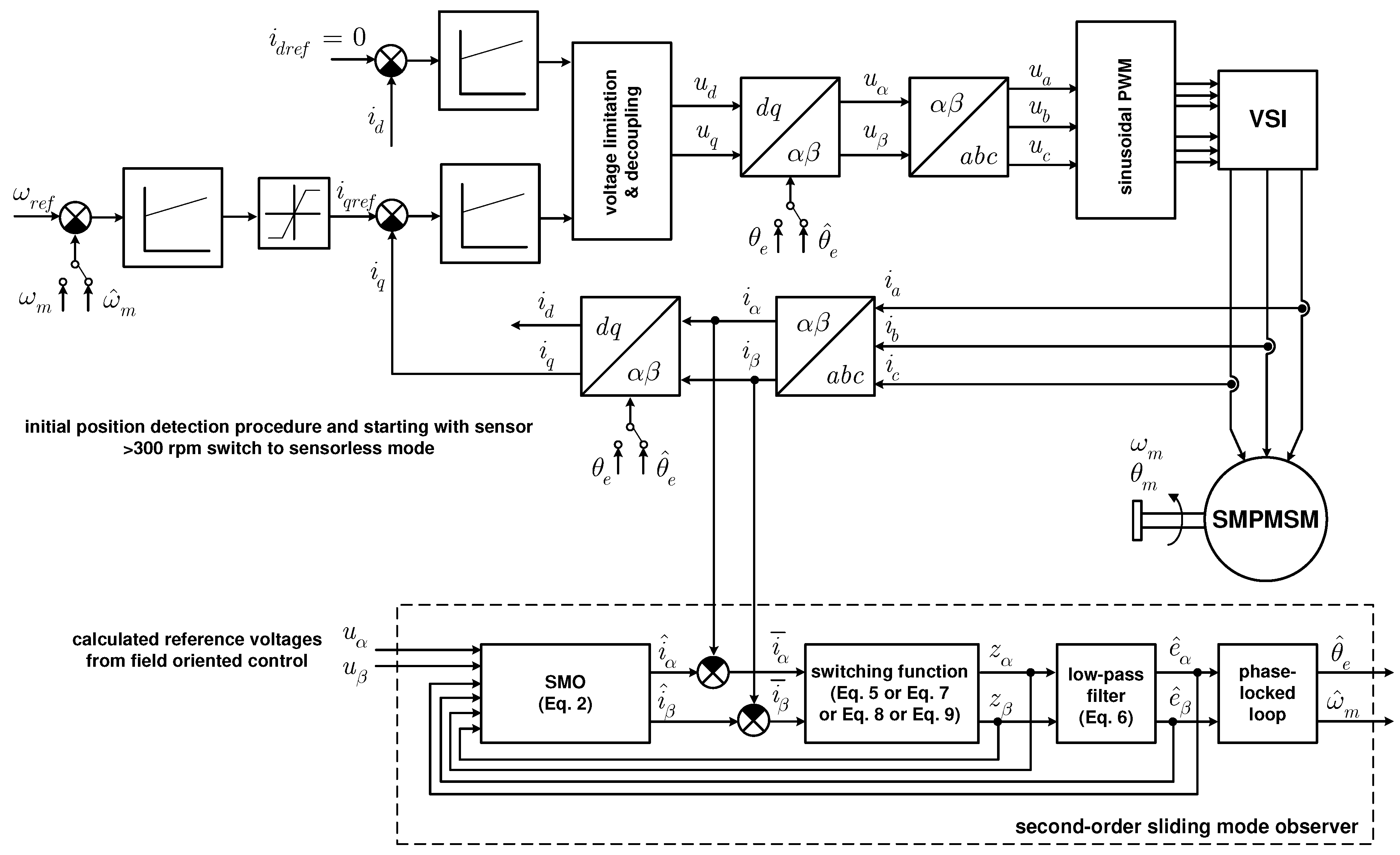
2. Implementation of SOSMO for Sensorless Control of PMSM

The state equation of SM-PMSM using the $\alpha \beta$ stator currents as state variables is defined as:

$$\left[\begin{array}{c}{\dot{i}}_{\alpha }\\ {\dot{i}}_{\beta }\end{array}\right]=\frac{1}{L_s}\left[\begin{array}{cc}-R_s& 0\\ 0& -R_s\end{array}\right]\left[\begin{array}{c}{i}_{\alpha }\\ i_{\beta }\end{array}\right]+\frac{1}{L_s}\left[\begin{array}{c}{u}_{\alpha }-e_{\alpha }\\ u_{\beta }-e_{\beta }\end{array}\right],$$

(1)

where $u_{\alpha }$ and $u_{\beta }$ are the applied stator voltage components, $i_{\alpha }$ and $i_{\beta }$ are the stator current components, $e_{\alpha }=-{\omega }_e{\lambda }_{PM}sin\left({\theta }_e\right)$ and $e_{\beta }={\omega }_e{\lambda }_{PM}cos\left({\theta }_e\right)$ are the stator back-EMF voltage components, where ${\omega }_e$ is the electrical angular velocity and ${\lambda }_{PM}=\frac{2}{3}\frac{k_t}{p}=\frac{k_e}{p}$ is the permanent magnet flux, where $k_t$ is the motor torque constant, $k_e$ is the EMF constant and p is the number of pole pairs, $R_s=R_{2ph}/2$, where $R_{2ph}$ is the phase-to-phase resistance and $L_s=L_{2ph}/2=L_d=L_q$, where $L_{2ph}$ is the phase-to-phase inductance and $L_d$, $L_q$ are the direct and quadrature axis inductances.

It can be seen from (1) that the back-EMF components include the value of rotor position and velocity. The amplitude of the back-EMF components cannot be directly measured during the control process and its estimation is thus required. A second-order sliding-mode observer (SOSMO) [41] is used in this paper for the speed and position estimation. The mathematical model of SOSMO can be defined as:

$$\left[\begin{array}{c}{\dot{\widehat{i}}}_{\alpha }\\ {\dot{\widehat{i}}}_{\beta }\end{array}\right]=\frac{1}{L_s}\left[\begin{array}{cc}-R_s& 0\\ 0& -R_s\end{array}\right]\left[\begin{array}{c}{\widehat{i}}_{\alpha }\\ {\widehat{i}}_{\beta }\end{array}\right]+\frac{1}{L_s}\left[\begin{array}{c}{u}_{\alpha }-{\widehat{e}}_{\alpha }-z_{\alpha }\\ u_{\beta }-{\widehat{e}}_{\beta }-z_{\beta }\end{array}\right],$$

(2)

where superscript (^) indicates an observed value and $z_{\alpha }$, $z_{\beta }$ are the observer feedback signals. If the actual motor parameters, i.e., the resistance and the inductance of the windings are the same as in the observer equations, the applied voltage components are known and the current components are measured, the only unknown values are the back-EMF components. Thus, matching the observed currents to the measured currents yields the actual back-EMF values. The observer’s task is to force the observed current to match the measured current, thus, the sliding surface is given as:

$$\mathbf{s}\left(t\right)=\left[\begin{array}{c}{\overline{i}}_{\alpha }\\ {\overline{i}}_{\beta }\end{array}\right]=\left[\begin{array}{c}{\widehat{i}}_{\alpha }-i_{\alpha }\\ {\widehat{i}}_{\beta }-i_{\beta }\end{array}\right],$$

(3)

where ${\overline{i}}_{\alpha }$, ${\overline{i}}_{\beta }$ represents the error between the observed and measured current components. The switching action will occur when:

$$\mathbf{s}\left(t\right)=0.$$

(4)

Equation (4) defines the sliding surface or the switching surface of the SOSMO. The phase plane is divided into two areas in which the switching function has different signs. The differences between actual and observed currents ${\overline{i}}_{\alpha }$, ${\overline{i}}_{\beta }$ enter the switching function. The outputs of the switching function are the feedback observer signals $z_{\alpha }$, $z_{\beta }$:

$$\left[\begin{array}{c}{z}_{\alpha }\\ z_{\beta }\end{array}\right]=f\left(\mathbf{s}\left(t\right)\right).$$

(5)

The back EMF-components are obtained by filtering the feedback observer signals with the LPF. The observed electrical position can be extracted from the estimated back-EMF components using an arctan function or a phase-locked loop (PLL) circuit. The latter is used in this paper and the design of the PLL can be found in [1].

The implementation of the SOSMO with the field-oriented control of PMSM is shown in Figure 1. The initial position detection and start-up are executed with a resolver. Then, above 10% of the nominal speed, the algorithm is switched to the sensorless mode. This approach is used to provide a fair comparison of different switching functions under exactly the same conditions for each measurement.

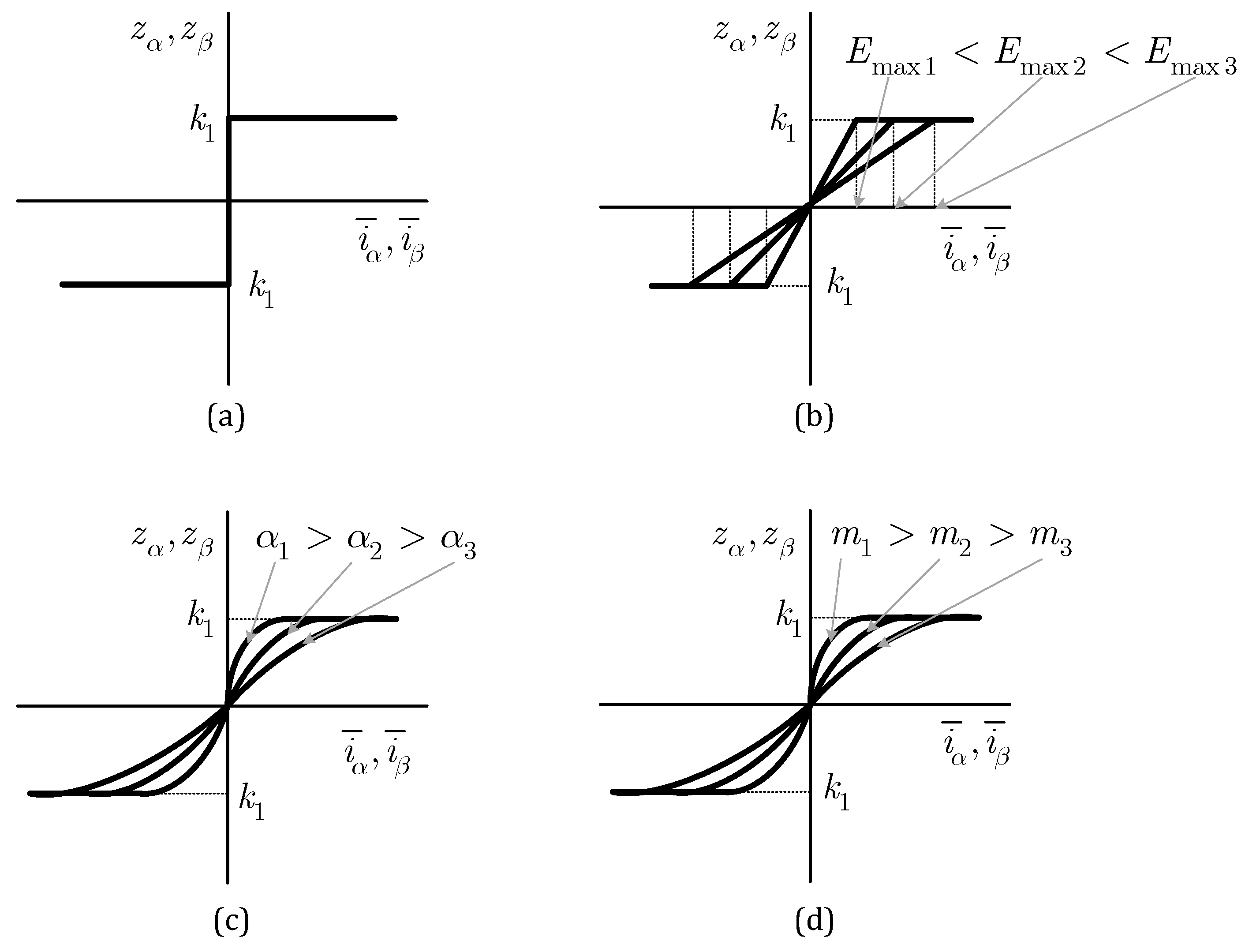
3. Classification of Switching Functions

Observer feedback signals $z_{\alpha }$, $z_{\beta }$ from the previous section can be calculated in different ways based on the type of switching function used in the control structure and the value of its shaping coefficient (SC). The switching function and value of the SC have a significant impact on the chattering of the observed values, having further impact on the performance of the sensorless drive. The purpose of the $z_{\alpha }$, $z_{\beta }$ signals is to force the trajectories of current differences ${\overline{i}}_{\alpha }$ and ${\overline{i}}_{\beta }$ towards the sliding surface. It was shown in several works that the discrete function (signum) causes chattering and so continuous functions are preferred. Different types of switching functions are shown in Figure 2.

3.1. Signum Function

The signum function is defined as follows:

$$\left[\begin{array}{c}{z}_{\alpha }\\ z_{\beta }\end{array}\right]=k_1\left[\begin{array}{c}\mathrm{sgn}\left({\overline{i}}_{\alpha }\right)\\ \mathrm{sgn}\left({\overline{i}}_{\beta }\right)\end{array}\right].$$

(6)

The sign of the current error is determined by the signum function and then multiplied by the feedback gain $k_1$. The value of $k_1$ is discussed in Section 3.5. The average value of the feedback signals from (6) in a short time interval represents the estimated back-EMF values [17]. Therefore, its components can be obtained using the LPF:

$$\left[\begin{array}{c}{\widehat{e}}_{\alpha }\\ {\widehat{e}}_{\beta }\end{array}\right]=\frac{{\omega }_c}{s+{\omega }_c}\left[\begin{array}{c}{z}_{\alpha }\\ z_{\beta }\end{array}\right],$$

(7)

where ${\omega }_c$ is the cut-off frequency of the LPF. For each type of switching function, the resulting observed back-EMF components are obtained using the LPF as defined in (7). The cut-off frequency is selected to filter out the high-frequency components, but ${\omega }_c$ should not affect the fundamental component of the feedback signal during the filtration process. The observed back-EMF components will be further used for the position and speed calculation. The LPF introduces a phase lag and a compensation of the observed position values is necessary [42].

For an ideal SOSMO, the signum function is executed with the infinite frequency and the trajectories of the current differences reach and stay on the sliding hyperplane, i.e., $\mathbf{s}\left(t\right)=0$ and $\dot{\mathbf{s}}\left(t\right)=0$. However, the switching frequency is limited in a real application, which is the reason why the chattering phenomenon occurs. To suppress the chattering of the observer, one of the available solutions is to use other types of switching function as a substitute for the signum function: saturation, sigmoid or hyperbolic function.

3.2. Saturation Function

The signum function is replaced by the saturation function. If the absolute value of the current differences ${\overline{i}}_{\alpha }$ and ${\overline{i}}_{\beta }$ is lower than a predefined value $E_{max}$ the feedback signal will change into a linear transient region [15]:

$$\left[\begin{array}{c}{z}_{\alpha }\\ z_{\beta }\end{array}\right]=\frac{k_1}{E_{max}}\left[\begin{array}{c}{\overline{i}}_{\alpha }\\ {\overline{i}}_{\beta }\end{array}\right].$$

(8)

The value of $k_1$ is discussed in Section 3.5. $E_{max}$ is a shaping coefficient for the saturation function.

3.3. Sigmoid Function

If a $\mathrm{sigmoid}$ function is used, the discontinuous signum function given by (6) is fully replaced by a continuous function $F\left(\overline{i}\right)$ and the observer feedback signals can be written as follows:

$$\left[\begin{array}{c}{z}_{\alpha }\\ z_{\beta }\end{array}\right]=k_1\left[\begin{array}{c}F\left({\overline{i}}_{\alpha }\right)\\ F\left({\overline{i}}_{\beta }\right)\end{array}\right],$$

(9)

where the function $F\left(\overline{i}\right)$ is defined as [43]:

$$F\left(\overline{i}\right)=\frac{2}{1+e^{-\alpha \overline{i}}}-1,$$

(10)

where $\alpha$ is the shaping coefficient of the sigmoid function. If the value $E_{max}$ in the saturation function is selected high enough, or if the value of $\alpha$ in the sigmoid function is selected small enough, the continuous output (i.e., observed back-EMF values) will be achieved even without the filtering by the LPF. This simplifies the control system and the compensation of LPF is not necessary anymore. However, removing the LPF reduces the dynamic performance of the observer due to the sluggish response of the controller.

3.4. Hyperbolic Function

The hyperbolic function is defined as follows:

$$\begin{array}{c}\hfill \begin{array}{c}\hfill \left[\begin{array}{c}{z}_{\alpha }\\ z_{\beta }\end{array}\right]=k_1\left[\begin{array}{c}\frac{e^{m\overline{i_{\alpha }}}-e^{-m\overline{i_{\alpha }}}}{e^{m\overline{i_{\alpha }}}+e^{-m\overline{i_{\alpha }}}}\\ \frac{e^{m\overline{i_{\beta }}}-e^{-m\overline{i_{\beta }}}}{e^{m\overline{i_{\beta }}}+e^{-m\overline{i_{\beta }}}}\end{array}\right],\end{array}\end{array}$$

(11)

where m is the shaping coefficient. The hyperbolic function defined by (11) belongs to the class of sigmoid functions but its SC is defined in a different manner [43]. However, it can be shown that the hyperbolic function can be applied as a substitute for the sigmoid function, if the following condition is met: $m=\frac{1}{2}\alpha$.

3.5. Feedback Switching Gain

The value of the feedback gain $k_1$ plays an important role in the observer’s performance and stability. The selection of $k_1$ for the the signum function can be found in [17], for the saturation function in [28] and for the sigmoid function in [43]. The following must stand to ensure stability for all three functions:

$$\begin{array}{c}\hfill \begin{array}{c}\hfill k_1>\max (\left|e_{\alpha }\right|,\left|e_{\beta }\right|).\end{array}\end{array}$$

(12)

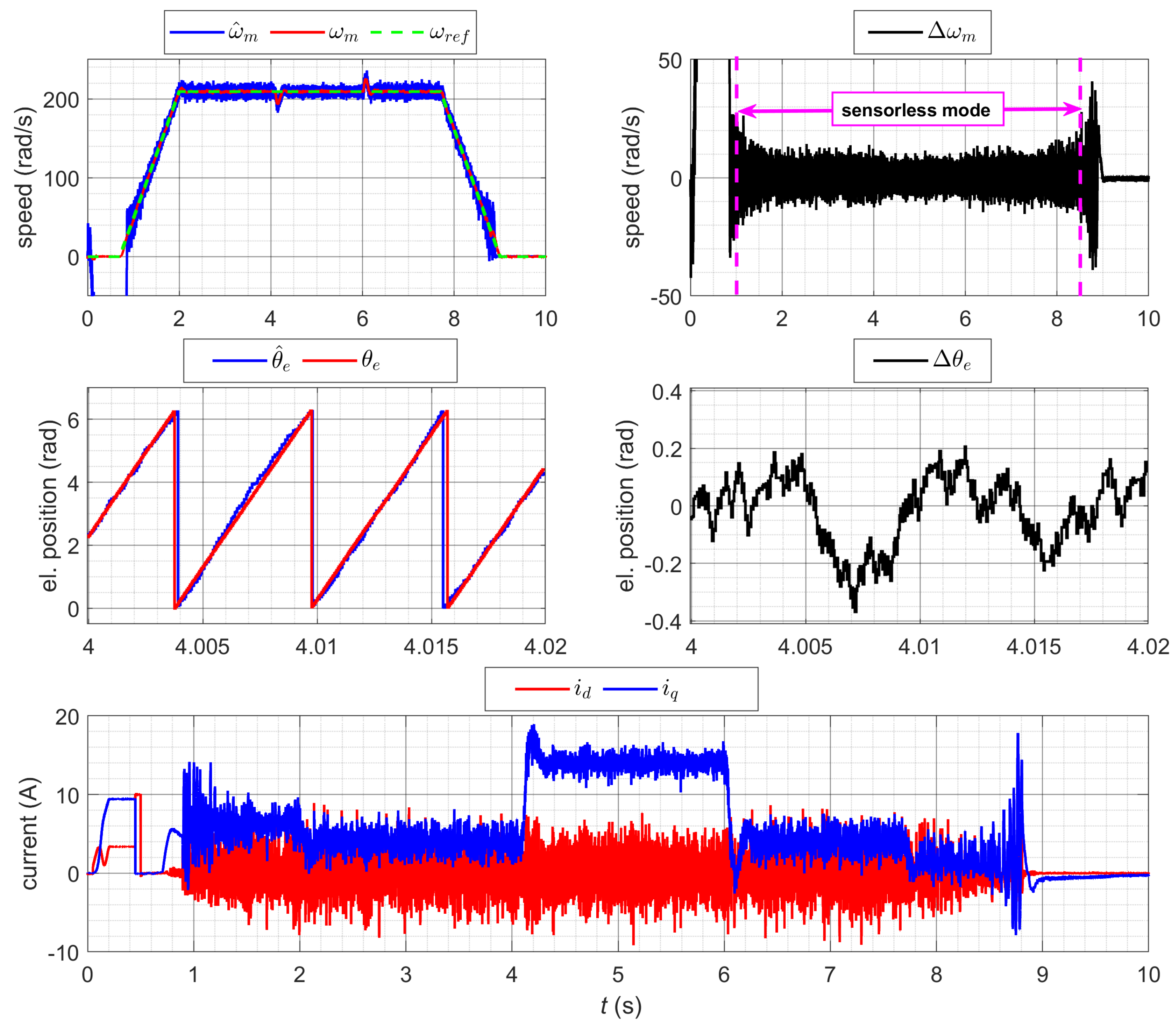
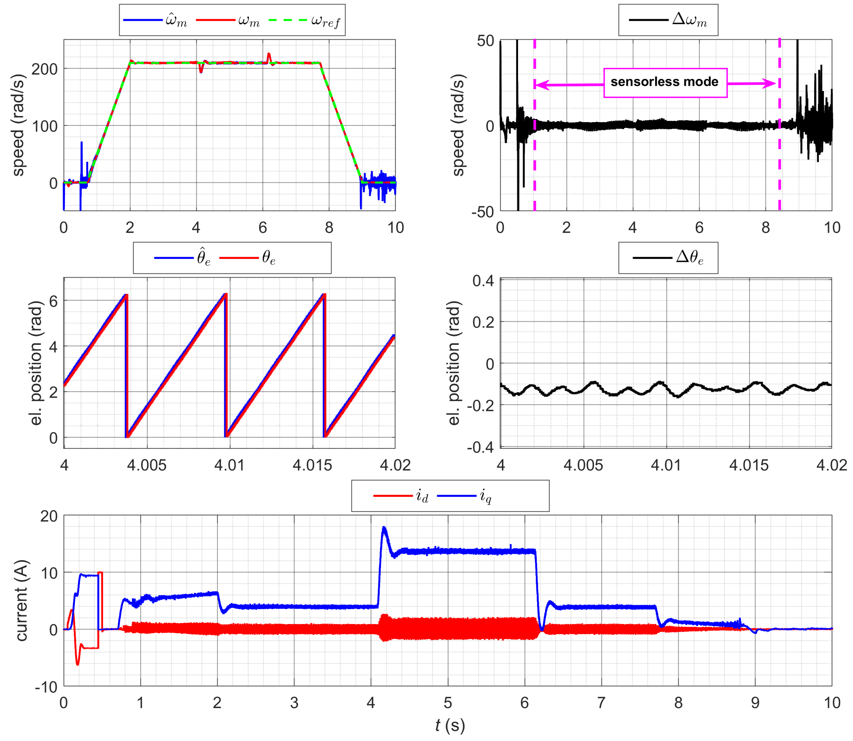
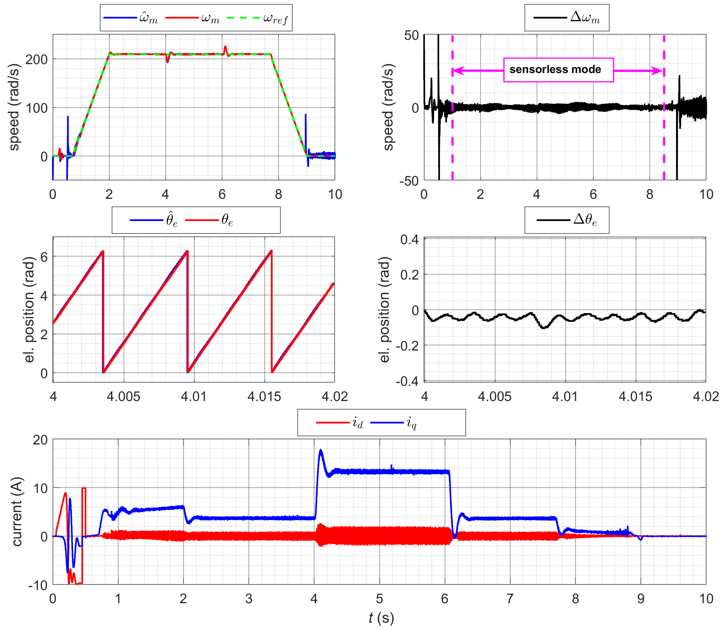
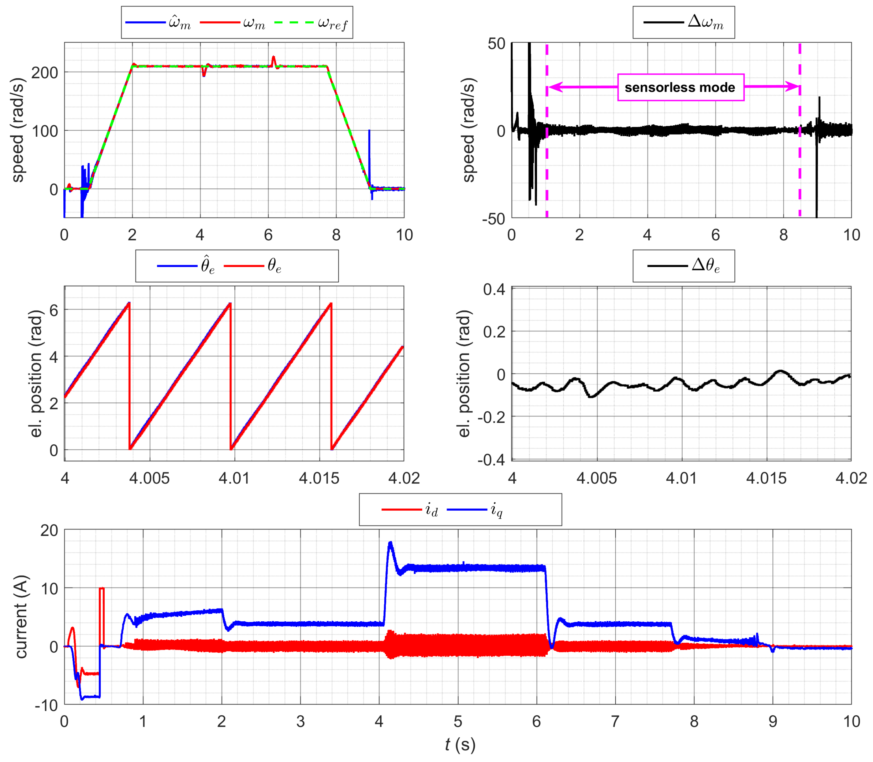
4. Experimental Results of Different Switching Functions in Sensorless Control

An SM-PMSM with the parameters shown in

Table 1. Parameters of PMSM and controllers.

Motor Type	TGN3-0115-30-48/T1
dc link voltage	$U_{DC}=48$ V
rated torque	$M_N=1.13$ Nm
rated current	$I_N=12.9$ A
torque constant	$k_t=0.101$ Nm/A
voltage constant	$k_e=6.12$ V/1000 rpm
no. of pole pairs	$p=5$
rated speed	$n_N=3000$ rpm
stator resistance	$R_{2ph}=0.258\Omega$
stator inductance	$L_{2ph}=0.6$ mH
PI speed controller	$k_P=0.05$
	$k_I=0.59$
PI current controller	$k_P=0.12$
	$k_I=86$
PLL	$k_P=1400$
	$k_I$ = 490,000
max. current	$I_{max}=18$ A
cut-off frequency of the LPF	$f_{LPF}$ = 7.7 kHz
feedback gain	$k_1$ = 100

was used for the experimental testing. A prototype of a voltage source inverter (VSI) controlled by an Opal RT OP5600 hardware-in-the-loop simulator was used to drive the machine. Two different sampling rates were implemented: the SOSMO and the current loop were sampled at 20 kHz and the speed control loop was sampled at a 2 kHz sampling frequency. The parameters of all controllers are shown in Table 1. The current controllers were designed by direct synthesis method for the desired time constant $T_n=1.5$ ms, which results in a bandwidth of approximately 670 Hz. The PI speed controller was initially designed for the operation with the sensor. Then, it was experimentally tuned in sensorless control by a trial-and-error approach and the P-component of the PI controller was reduced to make its value fit the full range of shaping coefficients for all switching functions. When a satisfactory value of the P-component was found, it was not changed throughout all experiments. This ensured the fairest possible comparison of switching functions.

The rotor position and speed estimation using the SOSMO observer are approximately reliable above 5–10% of the nominal speed. Therefore, some type of start-up procedure is required. In this paper, the position sensor was used to reach a certain speed level followed by the switch-over to sensorless control. This approach was chosen due to its simplicity, to accomplish a smooth initial position detection and to provide a fair comparison of all switching functions across all the values of SC. A switchover speed of 300 rpm was selected, which represents $10\%$ of the nominal speed. Below that speed, the observation fails, as the back-EMF amplitude has a critically low value to be reliably observable.

All four switching functions were experimentally tested with the same SOSMO, for the same parameters of the PI controller and with the same PLL circuit to provide the most objective comparison. For each measurement, the same level of a step load torque was applied to the PMSM by loading with the induction machine controlled by a frequency converter.

Different types of switching functions and SC were used. The results are shown in Figure 3, Figure 4, Figure 5 and Figure 6. The arrangement of all figures is the same:

• The upper left picture shows the actual and estimated speeds throughout the experiment;
• The upper right picture shows the calculated speed error $\Delta {\omega }_m={\omega }_m-{\widehat{\omega }}_m$ and indicates the sensorless operation area;
• The middle left picture shows a detail of the actual and estimated electrical position to see how accurate the position estimation is;
• The middle right picture shows a detail of the calculated electrical position error $\Delta {\theta }_e={\theta }_e-{\widehat{\theta }}_e$;
• The bottom picture shows the values of the actual $i_d$ and $i_q$ currents from the field oriented control.

Experimental results for the SOSMO implemented with a signum function are shown in Figure 3. The point of switchover from the sensor to sensorless control is visible at the time around $t=1$ s. A substantial chattering effect can be observed in the waveforms of the currents and actual speed, which makes this switching function the worst candidate for implementation in the sensorless control. The speed error $\Delta {\omega }_m$ has valid values only in the sensorless mode. Even if the estimated speed is calculated in both modes with sensor and sensorless, it has very unprecise values at low speeds, where the back-EMF voltages are very low.

The saturation function was experimentally tested for six different values of SC (see values of $E_{max}$ in

Table 2. Measured RMSE values for different switching functions and SC.

Switching Function	SC	RMSE ${\mathit{\omega }}_{\mathit{m}}$ (rad/s)	RMSE ${\mathit{\theta }}_{\mathit{e}}$ (rad)
hyperbolic	m = 0.002	0.735	0.323
hyperbolic	m = 0.004	0.799	0.167
hyperbolic	m = 0.008	0.865	0.066
hyperbolic	m = 0.012	0.890	0.058
hyperbolic	m = 0.016	0.893	0.079
hyperbolic	m = 0.02	0.901	0.070
hyperbolic	m = 0.024	0.906	0.094
hyperbolic	m = 0.028	0.904	0.100
hyperbolic	m = 0.032	0.900	0.106
hyperbolic	m = 0.04	0.899	0.094
saturation	$E_{max}$ = 20	0.913	0.128
saturation	$E_{max}$ = 25	0.922	0.110
saturation	$E_{max}$ = 30	0.927	0.094
saturation	$E_{max}$ = 35	0.916	0.096
saturation	$E_{max}$ = 40	0.915	0.095
saturation	$E_{max}$ = 45	0.911	0.110
sigmoid	$\alpha$ = 0.003	0.705	0.416
sigmoid	$\alpha$ = 0.03	0.885	0.061
sigmoid	$\alpha$ = 0.04	0.898	0.077
sigmoid	$\alpha$ = 0.05	0.903	0.105
sigmoid	$\alpha$ = 0.06	0.905	0.081
sigmoid	$\alpha$ = 0.08	0.912	0.112
signum	-	4.275	0.192

). Experimental results for the SOSMO with the saturation function $E_{max}$ = 20 are shown in Figure 4. When comparing Figure 3 and Figure 4, the chattering effect in the estimated speed is significantly reduced. In addition, the electrical position error $\Delta {\theta }_e$ is also reduced. The results in Figure 4 indicate that the saturation function has better performance in the sensorless control when compared with the signum function. However, it can be shown that the selection of some other values of $E_{max}$ may cause the chattering effect to reappear. It would be very convenient to find out the exact value of $E_{max}$ for which the chattering effect is minimal.

The sigmoid function was experimentally tested for six different values of SC (see values of $\alpha$ in Table 2). The experimental results for the SOSMO implemented with the signum function for $\alpha =0.04$ are shown in Figure 5. When comparing Figure 4 and Figure 5, the chattering effect in the current waveforms is at a comparable level, but the electrical position error is quite reduced. The results in Figure 5 indicate that the sigmoid function has slightly better performance in sensorless control when compared with the saturation function.

It should be again emphasized that a direct correlation between sigmoid and hyperbolic function exists. Based on a comparison of (9) with (11), it can be shown that $m=\frac{1}{2}\alpha$. Therefore, the sigmoid switching function can be used instead of the hyperbolic switching function and vice versa. This issue has not been discussed in the available literature so far.

The hyperbolic function was experimentally tested for 10 different values of SC (see values of m in Table 2). The experimental results for the hyperbolic function with $m=0.02$ are shown in Figure 6. The value of m was selected on purpose to compare the experimental results with the sigmoid function for $\alpha =0.04$. When comparing Figure 5 and Figure 6, no visible differences in chattering effect for the speed and current waveforms can be observed. The values of the mechanical speed and electrical position errors have a very similar level.

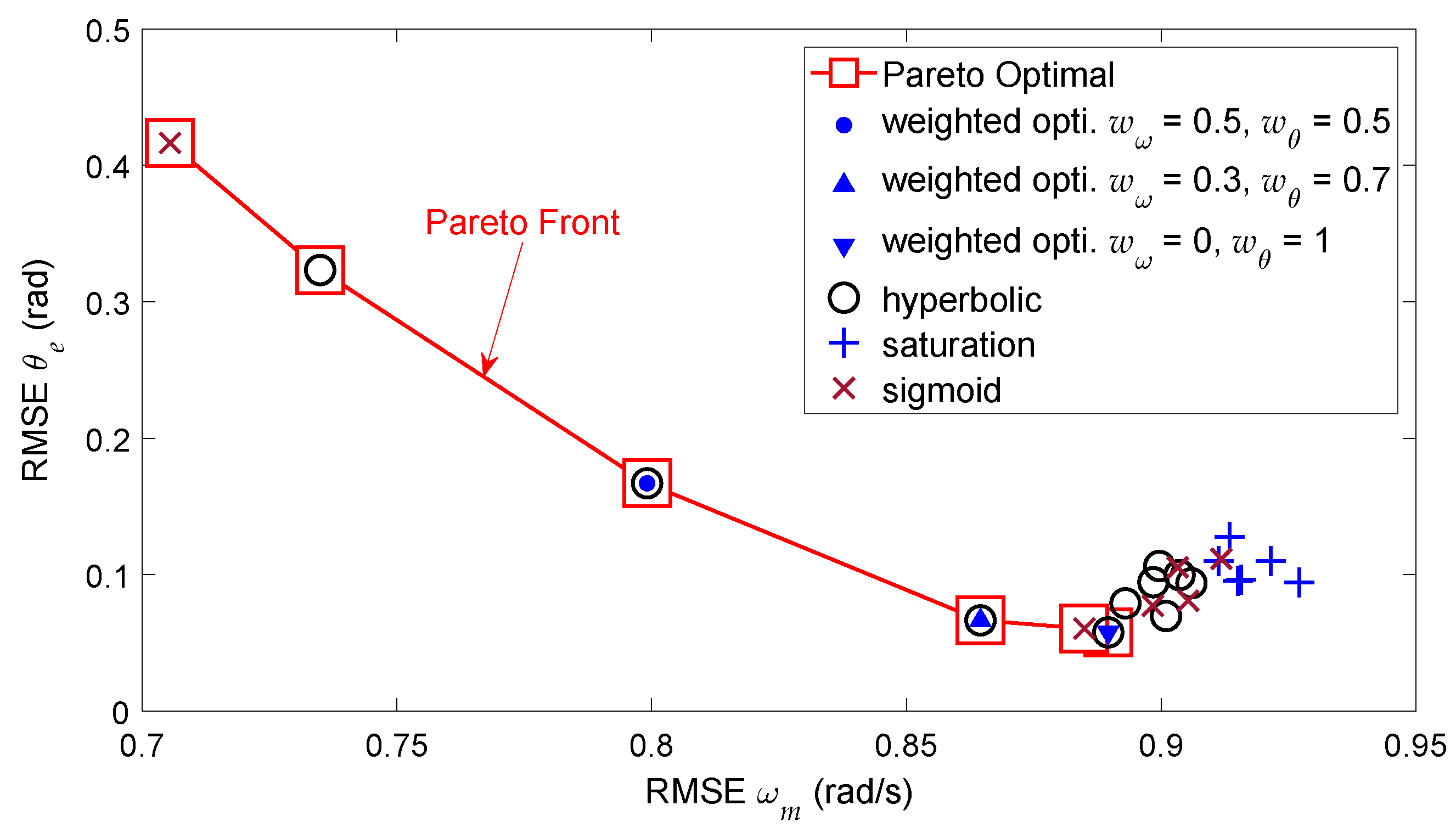
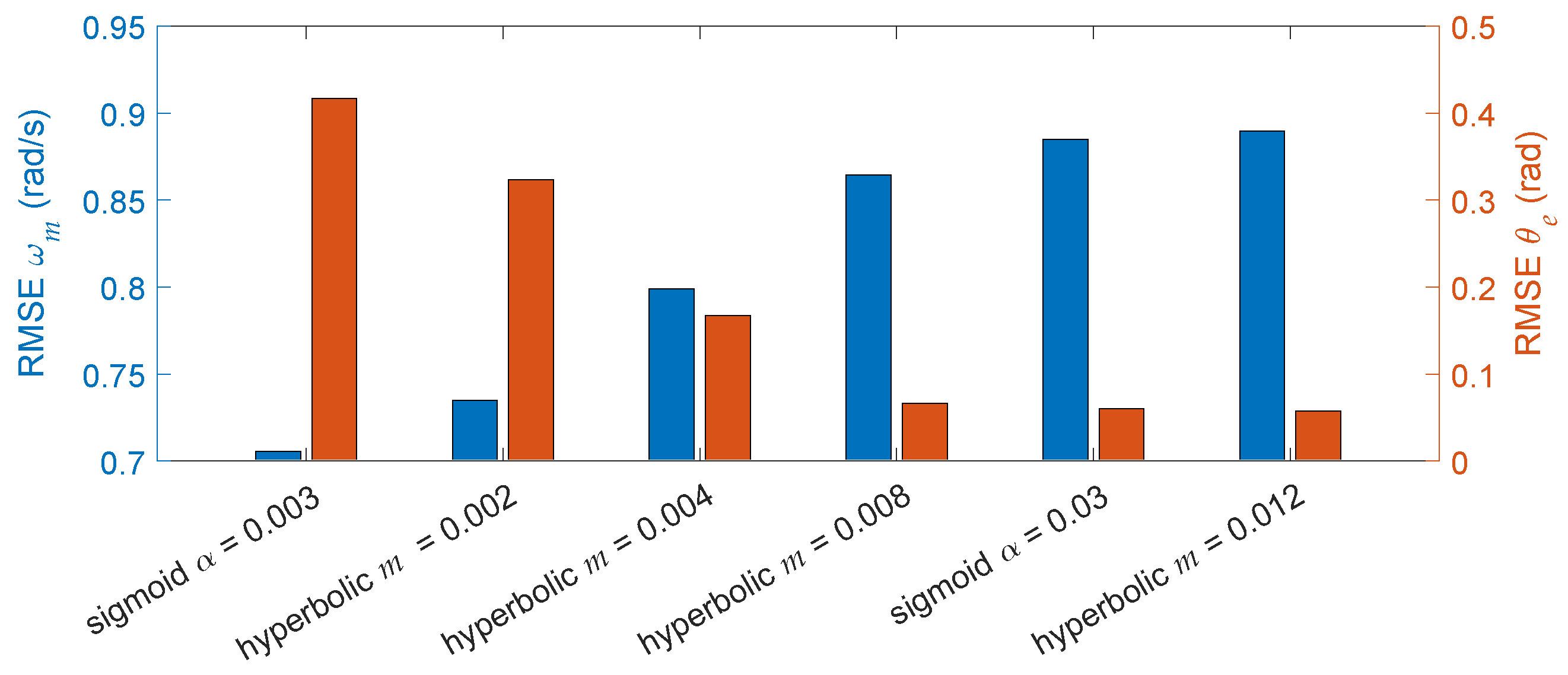
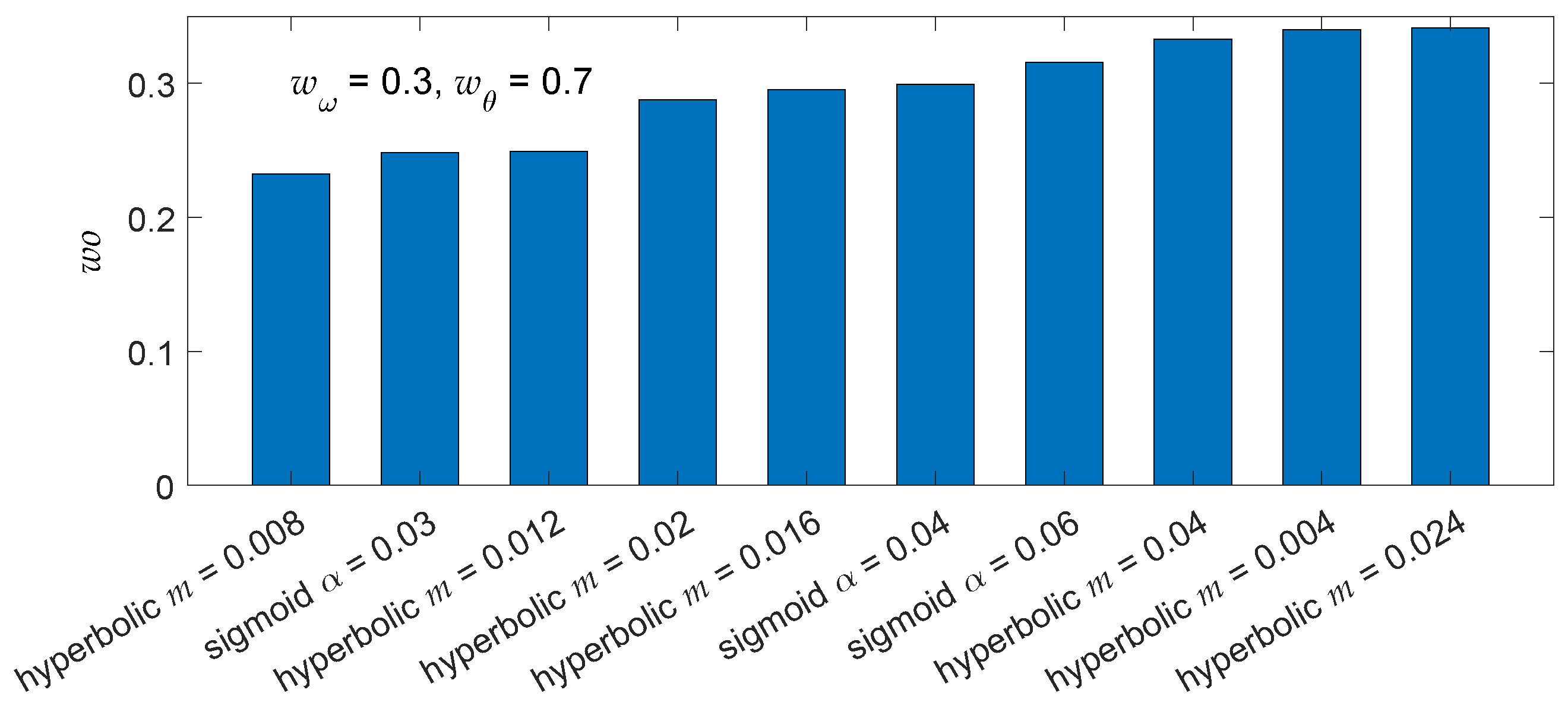
5. Multiobjective Optimization Problem for Values of SC

In the previous section, the comparison of the suitability of different switching functions was performed by evaluation of the speed, position and current responses. The values of SC were varied in order to reach the lowest possible chattering effect. Experimental results indicated that some optimal value of SC for each switching function should exist. Moreover, the comparison of SC only by visual examination of the speed, position and current waveforms is not enough to specify which value of SC is optimal. Therefore, some quantitative criterion must be introduced.

For most real-world problems, there are several objective functions (i.e., quantitative criteria) for comparing different solutions. These criteria are often conflicting as improving one leads to a deterioration of the other. Trying to find the “best” solution leads to two different approaches. The first is the multiple-criteria decision-making (MCDM) [44] that explicitly evaluates multiple conflicting criteria values of the finite set of possible solutions. The optimization model can be defined as:

$$\mathrm{minimize}\mathbf{q}$$

(13)

subject to

$$\mathbf{q}\in \mathbf{Q},$$

(14)

where $\mathbf{q}$ is the vector of p objective functions and $\mathbf{Q}$ is the set of alternative solutions.

The alternative approach is a multiobjective optimization (MOO) that uses various optimization methods to generate feasible solutions defined by the design parameters. The optimization model can be defined as [37]:

$$\mathrm{minimize}\mathbf{f}\left(\mathbf{x}\right):=\left[f_1\left(\mathbf{x}\right)f_2\left(\mathbf{x}\right),\cdots ,f_p\left(\mathbf{x}\right)\right],$$

(15)

subject to

$$g_i\le 0,i=1,2,\cdots ,m$$

(16)

$${\mathbf{x}}_l\le \mathbf{x}\le {\mathbf{x}}_u,$$

(17)

where $\mathbf{f}$ and $\mathbf{x}$ are an objective function vector and a design parameter vector, respectively; g and m are the constraints and number of constraints, respectively; and ${\mathbf{x}}_l$ and ${\mathbf{x}}_u$ are the lower and upper boundaries of $\mathbf{x}$.

In this paper, MCDM was used to select the best solution from the set of feasible solutions from the experiment. The MOO approach is not applicable because different switching functions have different shape coefficients and there is no uniform parameter space. MCDM compares different solutions to make the decision. In the case of multiple criteria, the evaluated objective of a solution is a vector. Two ways are offered to compare objective vectors and corresponding solutions.

The first defines the dominance of one solution over another [37]. The solution x dominates the solution y if the solution x is better than y in all criteria. The set of solutions that are not dominated by any solution in the set of feasible solutions is called the Pareto optimal set (or Pareto front). A simple search algorithm can be designed to find all Pareto optimal solutions from the existing set of feasible solutions.

The second approach reduces a multiobjective function to a single objective function by calculating one number as a weighted sum of objectives [45]. The best solution is the one with the lowest value (minimization problem). In this case, only one solution is optimal for a chosen set of weights. However, changing the weights leads to a different optimal solution. Both approaches were used in this paper.

Two different objective functions were selected: the root-mean-square error (RMSE) of the mechanical speed and the root-mean-square error of the electrical position, defined as follows:

$$\mathrm{RMSE}{\omega }_m=\sqrt{\frac{1}{n+1}\sum _{k=1}^n{\left(\Delta {\omega }_m\left(k\right)\right)}^2},$$

(18)

$$\mathrm{RMSE}{\theta }_e=\sqrt{\frac{1}{n+1}\sum _{k=1}^n{\left(\Delta {\theta }_e\left(k\right)\right)}^2},$$

(19)

where

$$\begin{array}{cc}\hfill \Delta {\omega }_m\left(k\right)& ={\omega }_m\left(k\right)-{\widehat{\omega }}_m\left(k\right),\hfill \end{array}$$

(20)

$$\begin{array}{cc}\hfill \Delta {\theta }_e\left(k\right)& ={\theta }_e\left(k\right)-{\widehat{\theta }}_e\left(k\right).\hfill \end{array}$$

(21)

$\Delta {\omega }_m\left(k\right)$ and $\Delta {\theta }_e\left(k\right)$ is a mechanical speed error and electrical position error, respectively; ${\omega }_e\left(k\right)$, ${\widehat{\omega }}_m\left(k\right)$ and ${\theta }_e\left(k\right)$, ${\widehat{\theta }}_e\left(k\right)$ are the kth samples of the actual and estimated mechanical speed and electrical position, respectively. n is the length of the dataset used for the calculation of the RMSE.

The weighted objective is the sum of the objectives according to (18) and (19). As the objectives have different scales, their normalization is necessary before the summing. The weighted objective $wo$ is calculated as:

$$\begin{array}{cc}\hfill wo& =w_{\omega }\frac{\mathrm{RMSE}{\omega }_m-min\left(\mathrm{RMSE}{\omega }_m\right)}{max\left(\mathrm{RMSE}{\omega }_m\right)-min\left(\mathrm{RMSE}{\omega }_m\right)}+w_{\theta }\frac{\mathrm{RMSE}{\theta }_e-min\left(\mathrm{RMSE}{\omega }_m\right)}{max\left(\mathrm{RMSE}{\theta }_e\right)-min\left(\mathrm{RMSE}{\theta }_e\right)},\hfill \end{array}$$

(22)

where $w_{\omega }$ and $w_{\theta }$ are weights and max(RMSEx), min(RMSEx) are extreme values of the objectives from all measurements.

Preliminary experiments were used to determine the range of shaping coefficients of the switching functions. Then, the full-scale experiments were executed as a series of repetitive measurements for exactly the same conditions (the same initial position detection, the same PI controller and PLL, and the same value of a load torque applied at the same time). A total of 319 experiments were executed, containing 138 measurements for the hyperbolic, 90 for the saturation, 90 for the sigmoid, and one measurement for the signum function to obtain statistically significant data for further investigation. A standard dataset had 12 measurements but three extended datasets of 30 measurements were executed to confirm the data normality required by statistical procedures. The possible erroneous values were identified and excluded from the datasets by a generalized extreme Studentized deviate test for outliers [46].

The values in Table 2 are the average of RMSEs obtained from the datasets for each single value of SC. The 95% confidence interval of values in Table 2 relative to measured RMSE ${\omega }_m$, or relative to 2$\pi$ for RMSE ${\theta }_e$, is ±0.3% on average, and ±0.5% in the worst case. This means that the true mean of the measured data lies within these intervals with a probability of 95% and it is not statistically significantly different from the average estimate.

Figure 7 shows the overview of the optimization results in the RMSE ${\omega }_m$ and RMSE ${\theta }_e$ space. Each solution is marked with one mark showing the switching function used and other marks showing whether the solution is Pareto optimal or optimal according to the weighted objective. The signum function is not displayed in the figure because the values of the objectives were very far from the optimum. Figure 8 shows the objective values of the Pareto optimal solutions in the same order from left to right as shown in Figure 7. The weighted objectives of the ten best solutions for weights $w_{\omega }=0.3$ and $w_{\theta }=0.7$ are shown in Figure 9.

As has been stated, hyperbolic and sigmoidal functions are interchangeable. The results of the experiments in Figure 7 confirm this statement although the overlapping of solutions is not accurate. The inaccurate overlap is a consequence of the fact that the SC values of $\alpha$ and m do not coincide with each other, as the measurement itself is random in nature. Considering this, we grouped together solutions that used the hyperbolic and sigmoid functions. After analyzing the optimization results we can state:

• The signum function gives the worst values of objective functions and serves only as a reference point.
• The solutions from the group of hyperbolic and sigmoid functions dominate over those of the saturation function.
• Multiobjective optimization gives several “good” solutions, so it is necessary to use additional preferences to select the best one.
• The optimal solutions according to the weighted objective lie on the Pareto front.

Based on the performed analysis, we lean toward the solution using the hyperbolic switching function with a shape coefficient m = 0.008 (sigmoid with $\alpha$ = 0.016). This is the optimal solution according to the weighted criterion with weights $w_{\omega }$ = 0.3 and $w_{\theta }$ = 0.7. The selected weights show that a smaller deviation of the electrical position than the deviation of the mechanical speed is preferred. The use of a saturation switching function is the second option if the time to calculate the hyperbolic function is unacceptable for given hardware. The fact that all Pareto optimal solutions belong to the same switching function (hyperbolic-sigmoid) opens the possibility for using M0O to search the exact SC value instead of selecting an optimal solution from the set of feasible ones. This may be the subject of future research.

6. Conclusions

This article has proposed a comparison of different switching functions and addresses the influence of their shaping coefficients on the performance of the sensorless control of PMSM. The results confirm that the signum function should be replaced with the sigmoid or hyperbolic function. This is caused by the utilization of the transient region of these switching functions, which enables the observer to exploit some additional “degree of freedom” during the observation process. It was proven that the sigmoid and hyperbolic switching functions are substitutable. In addition, a statistical evaluation of experiments with different values of shaping coefficients was completed by calculating the electrical position and mechanical speed root-mean-square-error values. Finally, a multiobjective optimization for given parameters resulted in several Pareto optimal solutions.

Future research should aim to add some more optimization objectives, such as speed settling time or overshoot, for a customization and expansion of the optimization problem. In addition, the shaping coefficients affect both the chattering effect and the robustness of the system. A selection of new optimization parameters that correlate with the robustness of the system is also viable.

References

1. Wang, G.; Guoqiang, Z.; Xu, D. Position Sensorless Control Techniques for Permanent Magnet Synchronous Machine Drives; Springer Nature: Singapore, 2020. [Google Scholar]
2. Wang, M.S.; Tsai, T.M. Sliding Mode and Neural Network Control of Sensorless PMSM Controlled System for Power Consumption and Performance Improvement. Energies 2017, 10, 1780. [Google Scholar] [CrossRef] [Green Version]
3. Infineon Technologies AG. XC886/888 CM/CLM 8-Bit Flash Microcontroller Sensorless Field Oriented Control for PMSM Motors, AP08059, Edition 2007-05. Available online: https://www.infineon.com/dgdl/AP0805910_Sensorless_FOC.pdf?fileId=db3a3043134dde6001134e2c3cff002f (accessed on 26 October 2021).
4. Cacciato, M.; Scarcella, G.; Scelba, G.; Bille, S.; Costanzo, D.; Cucuccio, A. Comparison of low-cost-implementation sensorless schemes in vector controlled adjustable speed drives. In Proceedings of the International Symposium on Power Electronics, Electrical Drives, Automation and Motion, Ischia, Italy, 11–13 June 2008; pp. 1082–1087. [Google Scholar] [CrossRef]
5. Microchip Technology. Sensorless FOC for PMSM Using Reduced Order Luenberger Observer AN2590. Available online: https://www.microchip.com/content/dam/mchp/documents/OTH/ApplicationNotes/ApplicationNotes/00002590B.pdf (accessed on 13 October 2021).
6. Tursini, M.; Scafati, A.; Guerriero, A.; Petrella, R. Extended Torque-Speed Region Sensor-Less Control of Interior Permanent Magnet Synchronous Motors. In Proceedings of the International Aegean Conference on Electrical Machines and Power Electronics, Bodrum, Turkey, 10–12 September 2007; pp. 647–652. [Google Scholar] [CrossRef]
7. Kivanc, O.C.; Ozturk, S.B. Sensorless PMSM Drive Based on Stator Feedforward Voltage Estimation Improved with MRAS Multiparameter Estimation. IEEE/ASME Trans. Mechatron. 2018, 23, 1326–1337. [Google Scholar] [CrossRef]
8. Abo-Khalil, A.G.; Eltamaly, A.M.; Alsaud, M.S.; Sayed, K.; Alghamdi, A.S. Sensorless control for PMSM using model reference adaptive system. Int. Trans. Electr. Energy Syst. 2021, 31, e12733. [Google Scholar] [CrossRef]
9. Bolognani, S.; Oboe, R.; Zigliotto, M. Sensorless full-digital PMSM drive with EKF estimation of speed and rotor position. IEEE Trans. Ind. Electron. 1999, 46, 184–191. [Google Scholar] [CrossRef]
10. Dilys, J.; Stankevič, V.; Łuksza, K. Implementation of Extended Kalman Filter with Optimized Execution Time for Sensorless Control of a PMSM Using ARM Cortex-M3 Microcontroller. Energies 2021, 14, 3491. [Google Scholar] [CrossRef]
11. Li, Y.; Wu, H.; Xu, X.; Sun, X.; Zhao, J. Rotor Position Estimation Approaches for Sensorless Control of Permanent Magnet Traction Motor in Electric Vehicles: A Review. World Electr. Veh. J. 2021, 12, 9. [Google Scholar] [CrossRef]
12. Filho, C.J.V.; Xiao, D.; Vieira, R.P.; Emadi, A. Observers for High-Speed Sensorless PMSM Drives: Design Methods, Tuning Challenges and Future Trends. IEEE Access 2021, 9, 56397–56415. [Google Scholar] [CrossRef]
13. Kung, Y.; Risfendra, R.; Lin, Y.; Huang, L. FPGA-realization of a sensorless speed controller for PMSM drives using novel sliding mode observer. Microsyst. Technol. 2016, 24, 79–93. [Google Scholar] [CrossRef]
14. Bilal, A.; Manish, B. Sensorless Field Oriented Control of 3-Phase Permanent Magnet Synchronous Motors, Application Report SPRABQ3. 2013. Available online: https://www.ti.com/lit/an/sprabq3/sprabq3.pdf (accessed on 26 October 2021).
15. Zambada, J.; Deb, D. Sensorless Field Oriented Control of a PMSM, AN1078 SPRABQ3. 2010. Available online: https://ww1.microchip.com/downloads/en/appnotes/01078b.pdf (accessed on 26 October 2021).
16. NXP. Sensorless PMSM Vector Control with a Sliding Mode Observer for Compressors Using MC56F8013, DRM099, Rev. 0. Available online: https://www.nxp.com/docs/en/reference-manual/DRM099.pdf (accessed on 26 October 2021).
17. Utkin, V.; Guldner, J.; Shi, J. Sliding Mode Control in Electro-Mechanical Systems; CRC Press: Boca Raton, FL, USA, 1999. [Google Scholar]
18. Baratieri, C.L.; Pinheiro, H. New variable gain super-twisting sliding mode observer for sensorless vector control of nonsinusoidal back-EMF PMSM. Control Eng. Pract. 2016, 52, 59–69. [Google Scholar] [CrossRef]
19. Liang, D.; Li, J.; Qu, R.; Kong, W. Adaptive Second-Order Sliding-Mode Observer for PMSM Sensorless Control Considering VSI Nonlinearity. IEEE Trans. Power Electron. 2018, 33, 8994–9004. [Google Scholar] [CrossRef]
20. Sreejith, R.; Singh, B. Sensorless Predictive Control of SPMSM-Driven Light EV Drive Using Modified Speed Adaptive Super Twisting Sliding Mode Observer with MAF-PLL. IEEE J. Emerg. Sel. Top. Ind. Electron. 2021, 2, 42–52. [Google Scholar] [CrossRef]
21. Slotine, J.J.E. Sliding controller design for non-linear systems. Int. J. Control 1984, 40, 421–434. [Google Scholar] [CrossRef]
22. Gong, C.; Hu, Y.; Gao, J.; Wang, Y.; Yan, L. An Improved Delay-Suppressed Sliding-Mode Observer for Sensorless Vector-Controlled PMSM. IEEE Trans. Ind. Electron. 2020, 67, 5913–5923. [Google Scholar] [CrossRef]
23. Ye, S.; Yao, X. An Enhanced SMO-Based Permanent-Magnet Synchronous Machine Sensorless Drive Scheme with Current Measurement Error Compensation. IEEE J. Emerg. Sel. Top. Power Electron. 2021, 9, 4407–4419. [Google Scholar] [CrossRef]
24. Liu, Y.; Fang, J.; Tan, K.; Huang, B.; He, W. Sliding Mode Observer with Adaptive Parameter Estimation for Sensorless Control of IPMSM. Energies 2020, 13, 5991. [Google Scholar] [CrossRef]
25. Song, X.; Fang, J.; Han, B.; Zheng, S. Adaptive Compensation Method for High-Speed Surface PMSM Sensorless Drives of EMF-Based Position Estimation Error. IEEE Trans. Power Electron. 2016, 31, 1438–1449. [Google Scholar] [CrossRef]
26. An, Q.; Zhang, J.; An, Q.; Liu, X.; Shamekov, A.; Bi, K. Frequency-Adaptive Complex-Coefficient Filter-Based Enhanced Sliding Mode Observer for Sensorless Control of Permanent Magnet Synchronous Motor Drives. IEEE Trans. Ind. Appl. 2020, 56, 335–343. [Google Scholar] [CrossRef]
27. Ye, S.; Yao, X. A Modified Flux Sliding-Mode Observer for the Sensorless Control of PMSMs with Online Stator Resistance and Inductance Estimation. IEEE Trans. Power Electron. 2020, 35, 8652–8662. [Google Scholar] [CrossRef]
28. Chi, S.; Zhang, Z.; Xu, L. Sliding-Mode Sensorless Control of Direct-Drive PM Synchronous Motors for Washing Machine Applications. IEEE Trans. Ind. Appl. 2009, 45, 582–590. [Google Scholar] [CrossRef]
29. Bao, D.; Wu, H.; Wang, R.; Zhao, F.; Pan, X. Full-Order Sliding Mode Observer Based on Synchronous Frequency Tracking Filter for High-Speed Interior PMSM Sensorless Drives. Energies 2020, 13, 6511. [Google Scholar] [CrossRef]
30. Lu, W.; Zheng, D.; Lu, Y.; Lu, K.; Guo, L.; Yan, W.; Luo, J. New Sensorless Vector Control System with High Load Capacity Based on Improved SMO and Improved FOO. IEEE Access 2021, 9, 40716–40727. [Google Scholar] [CrossRef]
31. Gao, W.; Zhang, G.; Hang, M.; Cheng, S.; Li, P. Sensorless Control Strategy of a Permanent Magnet Synchronous Motor Based on an Improved Sliding Mode Observer. World Electr. Veh. J. 2021, 12, 74. [Google Scholar] [CrossRef]
32. Liu, G.; Zhang, H.; Song, X. Position-Estimation Deviation-Suppression Technology of PMSM Combining Phase Self-Compensation SMO and Feed-Forward PLL. IEEE J. Emerg. Sel. Top. Power Electron. 2021, 9, 335–344. [Google Scholar] [CrossRef]
33. Kim, H.; Son, J.; Lee, J. A High-Speed Sliding-Mode Observer for the Sensorless Speed Control of a PMSM. IEEE Trans. Ind. Electron. 2011, 58, 4069–4077. [Google Scholar] [CrossRef]
34. Ren, N.; Fan, L.; Zhang, Z. Sensorless PMSM Control with Sliding Mode Observer Based on Sigmoid Function. J. Electr. Eng. Technol. 2021, 16, 933–939. [Google Scholar] [CrossRef]
35. Zhao, W.; Wang, X.; Gerada, C.; Zhang, H.; Liu, C.; Wang, Y. Multi-Physics and Multi-Objective Optimization of a High Speed PMSM for High Performance Applications. IEEE Trans. Magn. 2018, 54, 1–5. [Google Scholar] [CrossRef]
36. Diao, K.; Sun, X.; Lei, G.; Guo, Y.; Zhu, J. Multiobjective System Level Optimization Method for Switched Reluctance Motor Drive Systems Using Finite-Element Model. IEEE Trans. Ind. Electron. 2020, 67, 10055–10064. [Google Scholar] [CrossRef]
37. Lei, G.; Jianguo, Z.; Youguang, G. Multidisciplinary Design Optimization Methods for Electrical Machines and Drive Systems; Springer: Berlin/Heidelberg, Germany, 2016. [Google Scholar] [CrossRef]
38. Szczepanski, R.; Tarczewski, T.; Erwinski, K.; Grzesiak, L.M. Comparison of Constraint-handling Techniques Used in Artificial Bee Colony Algorithm for Auto-Tuning of State Feedback Speed Controller for PMSM. In Proceedings of the 15th International Conference on Informatics in Control, Automation and Robotics, ICINCO, INSTICC, Porto, Portugal, 29–31 July 2018; SciTePress: Setúbal, Portugal, 2018; Volume 1, pp. 269–276. [Google Scholar] [CrossRef]
39. Szczepanski, R.; Tarczewski, T.; Grzesiak, L.M. Application of optimization algorithms to adaptive motion control for repetitive process. ISA Trans. 2021, 115, 192–205. [Google Scholar] [CrossRef]
40. Petro, V.; Kyslan, K. A Comparative Study of Different SMO Switching Functions for Sensorless PMSM Control. In Proceedings of the International Conference on Electrical Drives and Power Electronics (EDPE), Dubrovnik, Croatia, 22–24 September 2021; pp. 102–107. [Google Scholar] [CrossRef]
41. Petro, V.; Kyslan, K. Design and Simulation of Direct and Indirect Back EMF Sliding Mode Observer for Sensorless Control of PMSM. Power Electron. Drives 2020, 5, 215–228. [Google Scholar] [CrossRef]
42. Ye, S. Design and performance analysis of an iterative flux sliding-mode observer for the sensorless control of PMSM drives. ISA Trans. 2019, 94, 255–264. [Google Scholar] [CrossRef]
43. Masoumi Kazraji, S.; Soflayi, R.; Bannae Sharifian, M.B. Sliding-Mode Observer for Speed and Position Sensorless Control of Linear-PMSM. Electr. Control Commun. Eng. 2014, 5, 20–26. [Google Scholar] [CrossRef] [Green Version]
44. Jahan, A.; Edwards, K.L.; Bahraminasab, M. 4-Multi-criteria decision-making for materials selection. In Multi-Criteria Decision Analysis for Supporting the Selection of Engineering Materials in Product Design, 2nd ed.; Jahan, A., Edwards, K.L., Bahraminasab, M., Eds.; Butterworth-Heinemann: Oxford, UK, 2016; pp. 63–80. [Google Scholar] [CrossRef]
45. Ghane-Kanafi, A.; Khorram, E. A new scalarization method for finding the efficient frontier in non-convex multi-objective problems. Appl. Math. Model. 2015, 39, 7483–7498. [Google Scholar] [CrossRef]
46. Grubbs, F.E. Procedures for Detecting Outlying Observations in Samples. Technometrics 1969, 11, 1–21. [Google Scholar] [CrossRef]
Figure 1. A block diagram of sensorless field oriented control with SOSMO and PLL.
Energies 15 02689 g001
Figure 2. Different types of switching functions: (a) signum, (b) saturation, (c) sigmoid and (d) hyperbolic.
Energies 15 02689 g002
Figure 3. Experimental results for speed and position estimation with signum function.
Energies 15 02689 g003
Figure 4. Experimental results for speed and position estimation with saturation function, E m a x = 20 .
Energies 15 02689 g004
Figure 5. Experimental results for speed and position estimation with sigmoid function, α = 0.04 .
Energies 15 02689 g005
Figure 6. Experimental results for speed and position estimation with hyperbolic function, m = 0.02 .
Energies 15 02689 g006
Figure 7. The overview of optimization results in the RMSE ω m and RMSE θ e space.
Energies 15 02689 g007
Figure 8. RMSE ω m and RMSE θ e values of the Pareto optimal solutions from Figure 7.
Energies 15 02689 g008
Figure 9. The best 10 values according to the weighted objective for w ω = 0.3 and w θ = 0.7.
Energies 15 02689 g009