Radial Magnetic Bearings for Rotor–Shaft Support in Electric Jet Engine

Abstract

New technologies are being developed to elaborate cutting-edge electrical jet engines to replace classical constructions. These new concepts consider the possibility of using electrical machines both as starters and generators, as well as suspension systems for the turbine shafts of aircraft engines. The paper will present mathematical analysis regarding active magnetic bearing (AMB) implementation for rotor–shaft support. This technology allows the elimination of friction forces between cooperating kinematic pairs (stator and rotor), reduces the adverse effects of classic bearings, and increases operating speed range and an operational susceptibility. The mathematical and numerical analysis of active magnetic suspension systems are presented. Next, a comparison of the theoretical studies using Comsol Multiphysics software and its experimental verification are described. A discussion regarding the mathematical analysis and experimental effects is also provided. The conclusion summarizes the theoretical and experimental features of heteropolar radial active magnetic bearings in new electric aircraft engines.

1. Introduction

Nowadays, the ecological requirements for new aircraft engines require the development of new technologies to replace classical engines with electrically supplied designs. This approach allows for the creation of environmentally friendly solutions. Therefore, aviation is also becoming an important field in which jet engines using aviation kerosene are planned to be replaced by jet engines powered by electricity [1]. However, due to the lack of efficient sources of electricity and the limitations related to its distribution, currently, such engines are mainly used to propel small, unmanned aerial vehicles.

In a classical jet engine, a turbine drives the compressor, which transmits propulsion through a shaft to the compressor [2]. However, in new electric jet engines, the compressor is driven by an electric drive, and the inverter controls the rotor speed. As a result, these new jet engines are considerably streamlined.

Bearing units are used to enable the cooperation of the rotating parts, i.e., rotors with compressors or rotors with electric drive, and the motor casing. Namely, bearings carry loads between the cooperating kinematic pair to reduce friction and remove heat from a rotor. Consequently, the bearings have to translate the radial and axial forces affected on the engine rotor–shaft. Thus, regardless of the powering method of an aircraft jet engine, bearings that support the rotor–shaft are crucial structural elements.

The rolling bearings typically applied in traditional jet engines are characterised by limitations that reduce the efficiency of the entire system and the reliability of its structure. This fact has been confirmed by so many literature items that it would be extremely troublesome to quote even some of them Namely, these bearings impose permissible values of maximum rotational speeds and limited tribological durability of the rolling elements, which entails the necessity to carry out relatively frequent and operationally troublesome repairs. In addition, rolling element bearings in jet engines require lubrication systems and additional cooling.

In addition to classic rolling bearings, alternatives of, for example, ceramic and hybrid bearings, have been tested [3]. Even though these bearings are resistant to corrosion, lack magnetic properties, are resistant to high and low temperature, electrically insulated, have no need for lubrication, and have lower unit weights and longer service lives than standard steel bearings, they still show the characteristic short-comings of rolling element bearings, which adversely affect the dynamic interactions of jet engine rotors with their housing. Moreover, as noted in [3], when monitoring their operation, they indicate only quantitative differences in terms of dynamic interaction in comparison to classic steel rolling bearings.

According to the above, compared to traditional rotor–shaft suspension methods using rolling element bearings and journal bearings, magnetic bearing arrangements have the following advantages [4,5]:

• The elimination of friction forces between cooperating elements, owing to the non-contact support of the rotor–shaft, ensures high durability of the journals and a lack of tribological wear;
• There is no need for lubrication, which, thanks to the removal of the lubrication system, significantly reduces the aircraft’s weight and shortens service time;
• Smaller radial stiffness, resulting in a reduction in critical speeds, owing to which there is a greater range of operating speeds at which the rotor–shaft tends to self-centre;
• Reduction in noise level and pollution generated by removing the lubrication system, which is a source of toxic materials that threaten the natural environment and operating personnel.

Moreover, magnetic suspensions are also characterized by significant load and rest capacity at high rotational speeds and better working parameters, especially at sudden, rapidly changing, dynamic, step-wise loads. Due to the properties mentioned above, magnetic suspensions are perfectly suited as supports for the rotor–shafts of jet engines powered by electricity. When applied to this type of jet engine, magnetic bearings can be divided into active bearings, passive bearings, and bearing-less electric motors, as described in [5,6,7,8].

Research on active magnetic bearings has been conducted intensively for at least three to four decades, and the number of published papers on this subject is so large that citing any of them seems troublesome here. According to ISO14839-1 [9], an active magnetic bearing is a mechatronic device that uses attractive or repulsive forces to ensure stable levitation of the rotor in the vicinity of the operating point. Active magnetic bearings use a feedback system that changes the value of the magnetic force generated by electromagnetic actuators [4,5,9]. Despite a need to use dedicated control systems to operate the active magnetic bearing, it provides precise control of the rotor position enabling an exact determination of its instantaneous position and ongoing monitoring and identification of the jet engine operating parameters. The main problems in the design of the active magnetic bearings are related to determining the stiffness coefficients of the electromechanical actuator and its transmission band. In addition, there are also issues in assessing the influence of the non-linear magnetic field on a stable operation of the active magnetic bearing. Most of them are related to the linearisation of the magnetic field non-linear model in the vicinity of the operating point, which is necessary during the analysis and synthesis of the active magnetic bearing control system [4].

In passive magnetic bearings, there is no system realising the feedback between the position of the rotor in the air gap and the value of the magnetic force. On the other hand, the force of magnetic levitation results from the interaction between molecular currents occurring in ordered structures, such as magnets, and the currents induced in conductors and superconductors [6,7]. Here, the source of the magnetic force is the molecular or induced currents that occur in diamagnetic, paramagnetic and permanent magnets. Generally, there are two basic types of passive magnetic bearings: permanent magnet static bearings and electro-dynamic bearings.

Passive magnetic bearings with permanent magnets are made of permanent magnets or sets of magnets arranged in appropriate arrays, e.g., Halbach’s arrays [6]. Their construction uses the forces of magnetic repulsion between two permanent magnets. Depending on the direction of the transferred loads, the design of these solutions uses magnets with different configurations of magnetisation vectors. Due to the limitations resulting from Earnshaw’s theorem, passive magnetic bearings for proper operation require additional systems limiting the number of degrees of freedom of the supported rotors. For this purpose, active magnetic bearings or classic bearing supports can be used [7].

In turn, in the passive electro-dynamic bearings, a source of the levitation force is the alternating magnetic field caused by mutual movement between the permanent magnets and the conductor in which currents are induced. Depending on the bearing design, permanent magnets are built into the housing, and the conductor is mounted on the shaft journal. Nevertheless, there are also reverse configurations. In both cases, an interaction between the induced current of the conductor and the magnetic field generates magnetic levitation forces. The most commonly used conductor materials are copper and aluminium.

The physical fundamentals of a dynamic rotary passive magnetic levitation can be found in [10,11]. In these papers, the mathematical modelling of the passive magnetic levitation is based on the solution of Maxwell equations. For small-size high-speed rotors, this approach has been applied in [12], where it results in the theoretical and experimental development of the radial electro-dynamic passive magnetic bearings, which sleeve-shaped rotating conductors characterise. Electro-dynamic passive magnetic bearings with disk-shaped conductors have further been modelled in [13,14] by applying Kirchhoff’s voltage law to the electrical circuits, including resistance and self-inductance of the conductor.

Since the condition for generating the electromagnetic levitation force is a presence of a relative velocity between the permanent magnets and the conductor, the electro-dynamic bearings cannot be used at rotor speeds close to zero Therefore, for each bearing, the minimum speed at which the generated magnetic force is greater than the rotor gravity is determined, and a magnetic levitation state is obtained.. Thus, a different type of bearing support is necessary at lower rotational speeds. According to the above, a prospective solution seems to be the development of a hybrid bearing consisting of the active magnetic bearing that functions as a support at low rotational speeds and the passive electro-dynamic bearing operating at high rotational speeds, in a similar way as, e.g., in [15].

Notably, we must remember that electro-dynamic passive magnetic bearings possess several disadvantages. These include their limited load capacity for supporting oversized rotors and poor damping abilities at high rotational speeds. Furthermore, these bearings can often cause operational instability. In order to avoid this drawback, and thus maintain the advantages mentioned above, the introduction of additional external damping into the rotor–shaft system is necessary. This problem was first raised in [10,11,12]. In [15], dynamic analysis was performed for the suspension of active magnetic bearings combined with permanent magnet static bearings, which were fitted to the rotor–shaft to stabilise its lateral vibrations. Static radial passive magnetic bearings and thrust electro-dynamic passive magnetic bearings were investigated in [6] for a vertical rotor–shaft, where mechanical touch-down bearings provided stabilisation. The notion of inserting additional damping into a radial electro-dynamic passive magnetic bearing supporting a rigid rotor is presented in [16,17], where they offer a combined passive–active magnetic support for rigid rotor–shafts, and [18], where external damping is generated passively. Various methods of introducing external damping and applying an active damper to stabilise flexible, high-speed rotors supported by electro-dynamic passive bearings were used in [19,20].

The last type of the mentioned magnetic suspensions are bearingless electric motors where torque and suspension windings are embedded. This technology has been widely researched and developed, especially to achieve high-speed drive in industrial applications. The latest papers have shown new control methods of bearingless induction motors [21,22], as well as the design and analyses of synchronous reluctance motors [23].

This paper will explain the concept of magnetic bearing systems for jet engines in detail. This concept is based on the implementation of active magnetic bearings and bearing-less electric drive technologies evolved in the Avionics Department at the Military University of Technology. The content of this paper is organised as follows: in the first section, the active magnetic bearing theory and model is introduced. Next, the theoretical studies using Comsol Multiphysics software and experimental verification are presented. The third section presents a discussion of the conducted experiments. Finally, concluding remarks based on the achieved results are given.

2. Study Object: Radial Active Magnetic Bearing

The magnetic support of high-speed rotors allow new electric jet engines to be designed. This new bearing concept for the rotor of electric jet engines includes two radial bearings and one axial bearing, as shown in Figure 1. Radial bearings regarding active or passive magnetic bearings can be put in different configurations, namely, they could be placed symmetrically towards a compressor, or asymmetrically behind the jet engine compressor. It should be mentioned here that the various concepts of magnetic support for the fluid flow machine rotor driven by an electric motor presented below may be used not only in aviation, but also in industrial blowers, compressors, vacuum pumps, precise high-speed lathes, and many other similar devices.

2.1. Active Magnetic Bearing Theory

Active magnetic bearings achieve stable magnetic levitation by using a feedback system that might change the value of the magnetic force in the air gap. This type of suspension consists of an electromechanical actuator, a sensor that determines the position of the mass in the air gap, and a control system. A non-contact eddy-current sensor detects a shaft raceway position change which is sent to the controller. Then, it will change the value of the magnetic force generated by the electromechanical part of the bearing by changing the current flowing in the windings. The value of the magnetic force changes actively and directly depending on the mass position in the air gap. The diagram of the control loop of the rotor position in the air gap is presented in Figure 2. The current changes take place according to the control law of the controller. In this way, a control system counteracts the shaft raceway movement in the air gap. An active magnetic suspension is always realised in a differential system and consists of two electromechanical actuators and two power amplifiers. In Figure 2a, the rotor–shaft raceway is placed at the operation point. Air gaps x₀ between the pole pieces and the rotor–shaft raceway are equal, and the current of the operation point i₀ supplies the down and upper electromagnets. The current flows in the electromagnets produce the electromagnetic forces F₀ of the same value, but in the opposite direction (marked by the green arrows). At the same time, air gap values are different if the rotor–shaft raceway moves from the operation point. Information about rotor–shaft raceway displacement will be registered by a sensor and transferred to the control unit, where control current i will be calculated. In Figure 2b, the rotor–shaft raceway is below its operation point; so, in the upper electromagnet, calculated current i would be added to the operation point current i₀, and in a down electromagnet, current i would be subtracted from the current i₀.

This paper’s subject is the theoretical and experimental analysis of parameters of the heteropolar radial active magnetic bearing. Any point on the rotor–shaft raceway perimeter in the heteropolar system passes four-fold electromagnets at the north pole and four-fold electromagnets at the south pole during one complete rotation. Alternating magnetic fields induce eddy currents. Thus, a track made of a soft magnetic sheet separated by a varnish layer set on the rotor–shaft raceway is required.

A determination of an electromechanical actuator stiffness, bandwidth setting, and the non-linear influence of the magnetic field distribution on the stable operation of the bearing magnetic field are the main problems that occur during magnetic bearing implementation. Most of the problems associated with estimating the above parameter are caused by the linearisation of the non-linear model. The linear model of the active magnetic bearing is determined to analyse and synthesise the individual bearing control systems and magnetic bearing systems of rigid and flexible rotors. In the case presented in Figure 2b, the electromagnetic force F₁ generated by the upper electromagnet is a non-linear function of control current i and rotor displacement x, and it can be expressed by:

$$F_1\left(i,x\right)=\frac{K}{4}\frac{{\left(i_0+i\right)}^2}{{\left(x_0-x\right)}^2}cos\alpha ,$$

(1)

where K is the bearing constant depending on coil turns, the electromagnet cross-section, and the magnetic permeability of the vacuum. Symbol α denotes the angle between the symmetry axis of the magnetic bearing and the axis of the pole piece.

In turn, the electromagnetic force generated by the lower electromagnet F₂ is described by Equation (2):

$$F_2\left(i,x\right)=\frac{K}{4}\frac{{\left(i_0-i\right)}^2}{{\left(x_0+x\right)}^2}cos\alpha$$

(2)

Thus, the resultant electromagnetic force acting on the levitated rotor in a vertical direction is equal:

$$F\left(i,x\right)=F_1\left(i,x\right)-F_2\left(i,x\right)=\frac{K}{4}\frac{{\left(i_0+i\right)}^2}{{\left(x_0-x\right)}^2}cos\alpha -\frac{K}{4}\frac{{\left(i_0-i\right)}^2}{{\left(x_0+x\right)}^2}cos\alpha .$$

(3)

The resultant electromagnetic force after linearisation in the operation point, presented in Figure 2a for i= 0 and x = 0, can be expressed by:

$$F\left(i,x\right)=k_{i}i+k_{x}x,$$

(4)

$$k_i=K\frac{i_0}{x_0^2}cos\alpha ,k_x=K\frac{i_0^2}{x_0^3}cos\alpha$$

(5)

where $k_i$ denotes the bearing current stiffness, and k_x is the bearing displacement stiffness described by expressions (5), respectively. Equation (4) can also be calculated using the virtual displacement method described in [24].

Determining the real values of current stiffness and displacement stiffness for a magnetic bearing is a challenging and complex issue. For that reason, the paper presents a theoretical and experimental analysis of these parameters.

2.2. AMB Model in Comsol Multiphysics Software

The discrete circuit model of AMB was presented in Section 2.1. This approach is shown above, giving an approximate solution. This solution is good enough to design the active magnetic bearing. However, the discrete circuit model does not include the non-linear property of magnetic material. The non-parametric model of the active magnetic bearing is more realistic than the discrete circuit model. This model was obtained based on the finite element method (FEM) using the Comsol Multiphysics software.

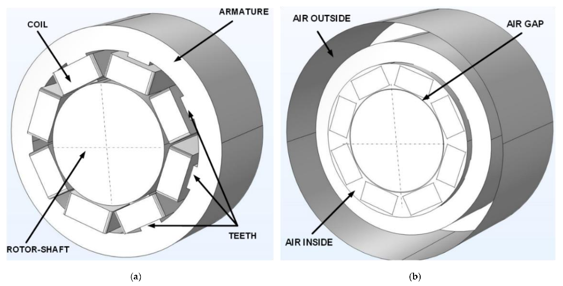
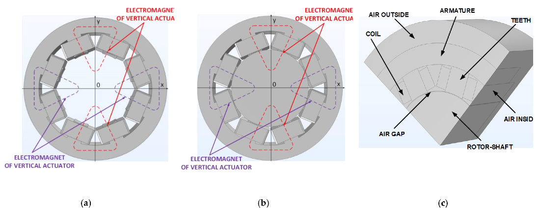
The model of the magnetic bearing includes a stator of the bearing, a rotor—shaft, electromagnetic coils, an air gap, and air around the bearing and inside the bearing. The stator of the active magnetic bearing is divided into an armature and teeth (Figure 3). The first step of the designing model is to generate geometrical shapes of the radial active magnetic bearing components. There are two electromagnetic actuators, which are presented in Figure 4. The construction of the actuator is described in Section 2.1.

The radial magnetic bearing has a symmetrical structure and symmetrical distribution electromagnetic properties. An exchange of electromagnetic energy between electromagnets is not observed. Therefore, the geometrical shapes of the bearing components illustrated in Figure 3 can be reduced to their one-eights, as shown in Figure 4c.

The next step to build the model is a definition of the physical properties. The armature of the stator, the teeth and the magnetic race (the element of the rotor–shaft) are made of silicon steel ET140-30. The silicon steel has the non-linear characteristic B-H (Figure 5). The coils of the electromagnets are made of copper wire with a diameter of 1.2 mm. The coil has 30 windings, and two coils are used in the electromagnet. The properties of the air are added for the air gap, i.e., the air-inside bearing and the air-outside bearing.

The program Comsol Multiphysics uses the Magnetic Field interface to compute magnetic field distributions around coils, conductors, and magnets. This interface solves Maxwell’s equations formulated using the magnetic vector and the scalar electric potential. The Magnetic Isolation node defines the boundary conditions of the magnetic model. The node is a special case of the magnetic potential boundary condition that sets the tangential component of the magnetic potential to zero:

$$n\times A=0,$$

(6)

where $n$ is the tangential component and $A$ is the magnetic potential.

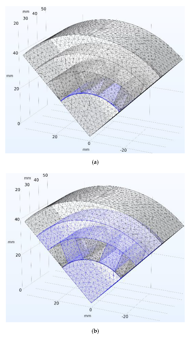
A division into three air groups is a result of the discretisation of space (Figure 6). The nominal air gap equals 0.25 mm, and this space is more important in the bearing model (Figure 6a). The mesh must be dense, and the triangle elements small enough. The next groups have larger-sized triangle elements. This approach simplifies the bearing model.

The magnetic field model can be used to obtain the non-parametric model of the radial active magnetic bearing. The model is written by the following equations:

$$\nabla \times H=J,$$

(7)

$$B=\nabla \times A,$$

(8)

$$J=\sigma E,$$

(9)

where H is the magnetic field, B denotes the magnetic flux density, A is the magnetic vector potential, E denotes the electric field, J is the density of the electric current, $\sigma$ denotes the conductivity and $\nabla$ is the nabla operator.

The magnetic properties of silicon steel are described by the equation:

$$B=f\left(\Vert H\Vert \right)\frac{H}{\Vert H\Vert },$$

(10)

where $\Vert H\Vert$ denotes the norm of the magnetic field and the B is the magnetic field read from the curve B-H (Figure 5).

The magnetic properties of the air and the copper coils are described by the equation:

$$B={\mu }_0{\mu }_{r}H$$

(11)

where ${\mu }_0$ denotes the vacuum permeability and ${\mu }_r$ is the relative permeability.

The basic geometrical dimensions and coil parameters of the active magnetic bearing are presented in

Table 1. Basic parameters of the AMB.

Parameters	Symbol	Value	Unit
Stator outer diameter	d2	90	mm
Stator inner diameter	d1	48	mm
Stator length	l	40	mm
Air gap (operation point)	x0	0.25	mm
Pole area	A	374.4	mm2
Coil turns	N	30	-
Max. current for operation point	i0	4	A

.

This model was obtained for the operation point defined by current i₀ and the air gap x₀. The resultant current in the electromagnet coil is a summation of the current in the operation point and control current i. The control current changes from −i₀ to i₀.

3. Results

3.1. Theoretical Studies with the Use of Comsol Multiphysics Software

The model of the active magnetic bearing was used to obtain the distribution of magnetic field, magnetic flux density, electromagnetic forces, and current in the coils of an electromagnet. The non-parametric model was obtained for different rotor displacements in the air gap and control current.

The first stage was the validation of the magnetic property of the magnetic bearing. In this stage, the electromagnet coils were supplied by the current control ranging from −1.5 A to 1.5 A. The resultant current in the coils were changed from 0 A to 3 A. The resultant current of the coil was obtained for the operation point current of 1.5 A:

$$i_{result}=i_0+i_{cont}$$

(12)

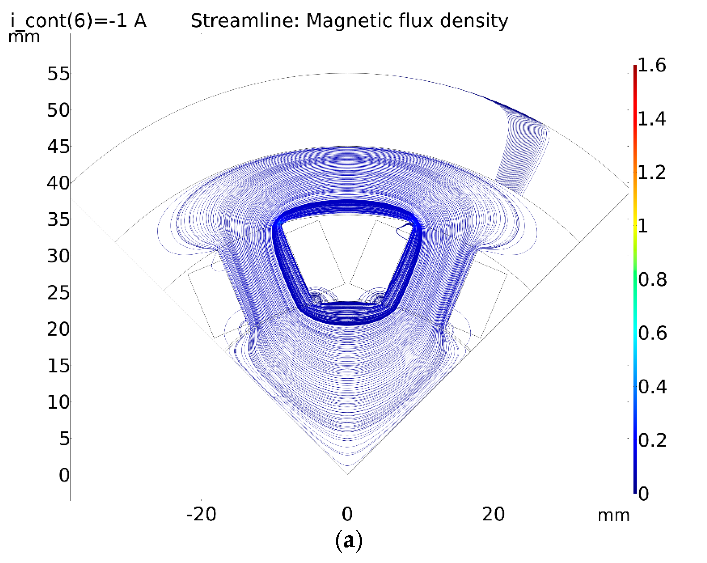
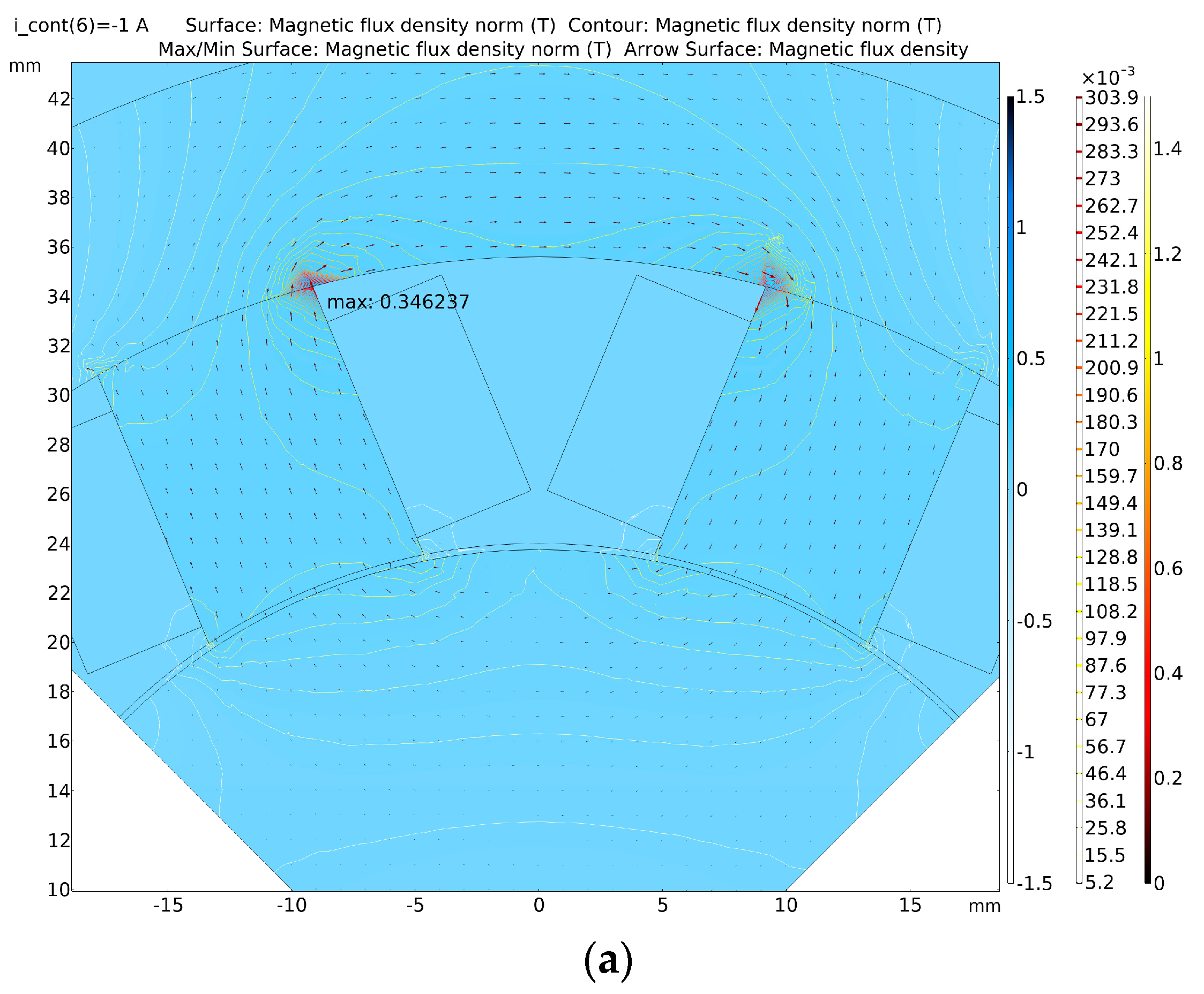
Figure 7 presents the distribution of the current density in the coils. The direction of current in the coils is a crucial parameter for the model. There were two coils in the electromagnet. The coils must be connected in series and ensure magnetic flow flux between the electromagnet poles. If the coils are incorrectly connected or have a wrong direction of current magnetic flux density, the magnetic path is reduced to zero. The next important property is ensuring the constant magnetic polarity of the electromagnet in the full range of the control current. Figure 8 shows the distribution of magnetic flux density. The streamlines ensure the magnetic flow flux has the same direction and the value of flux changes depending on the control current. Figure 9 presents the distribution of the module magnetic flux density. Figure 8 and Figure 9 show the magnetic flux concentration in the cross-section teeth and armature. There are strong concentration lines in the corners. This phenomenon is known as the magnetic notch. The analysis results show that the tested magnetic bearing had a strong magnetic notch and the bearing value of the cross-section was enough to ensure the magnetic and electrical parameters of the mechanical properties of the bearing. The distribution of magnetic flux density along the length of a magnetic bearing is presented in Figure 10.

The magnetic parameters for different control currents are presented in Figure 11. Those parameters were obtained along with a symmetry axis of the teeth. The axis was perpendicular to the rotor–shaft axis of symmetry. Figure 11a shows the distribution of the magnetic flux density. However, the magnetic field had an impulse in the air gap (radius from 23.75 to 24 mm), as seen in Figure 11b. This impulse came from moving the magnetic flux by a zone of high magnetic resistance (the air gap). The bearing stator and the magnetic race of the rotor–shaft were made of silicon steel. The magnetic resistance of air is greater than steel. Thus, a strong difference in magnetic potential was observed between the rotor and the pole of the electromagnet. The large magnetic resistance of the air reduced the magnetic flux density in the air gap, as is presented in Figure 11a.

Moreover, moving magnetic flux from the cross-section of the rotor to the cross-section of teeth influences the distribution of magnetic flux density.

The non-parametric model in the Comsol Multiphysics software allows verification of the bearing design and enabled us to obtain the mechanical properties of the radial forces. So, in the next stage, static characteristics of the bearing were obtained. Such static characteristics are the base for preparing the control system of the magnetic bearing.

The static characteristics were obtained as a function of the control current for different displacements of the rotor–shaft raceway in the air gap. The non-parametric model determines the magnetic forces which support the rotor shaft. The actuator of the magnetic bearing consists of two electromagnets, so the model calculates magnetic forces generated by the upper and lower electromagnets and the resultant differential magnetic force as:

$$F_{result}=F_{up}-F_{down}$$

(13)

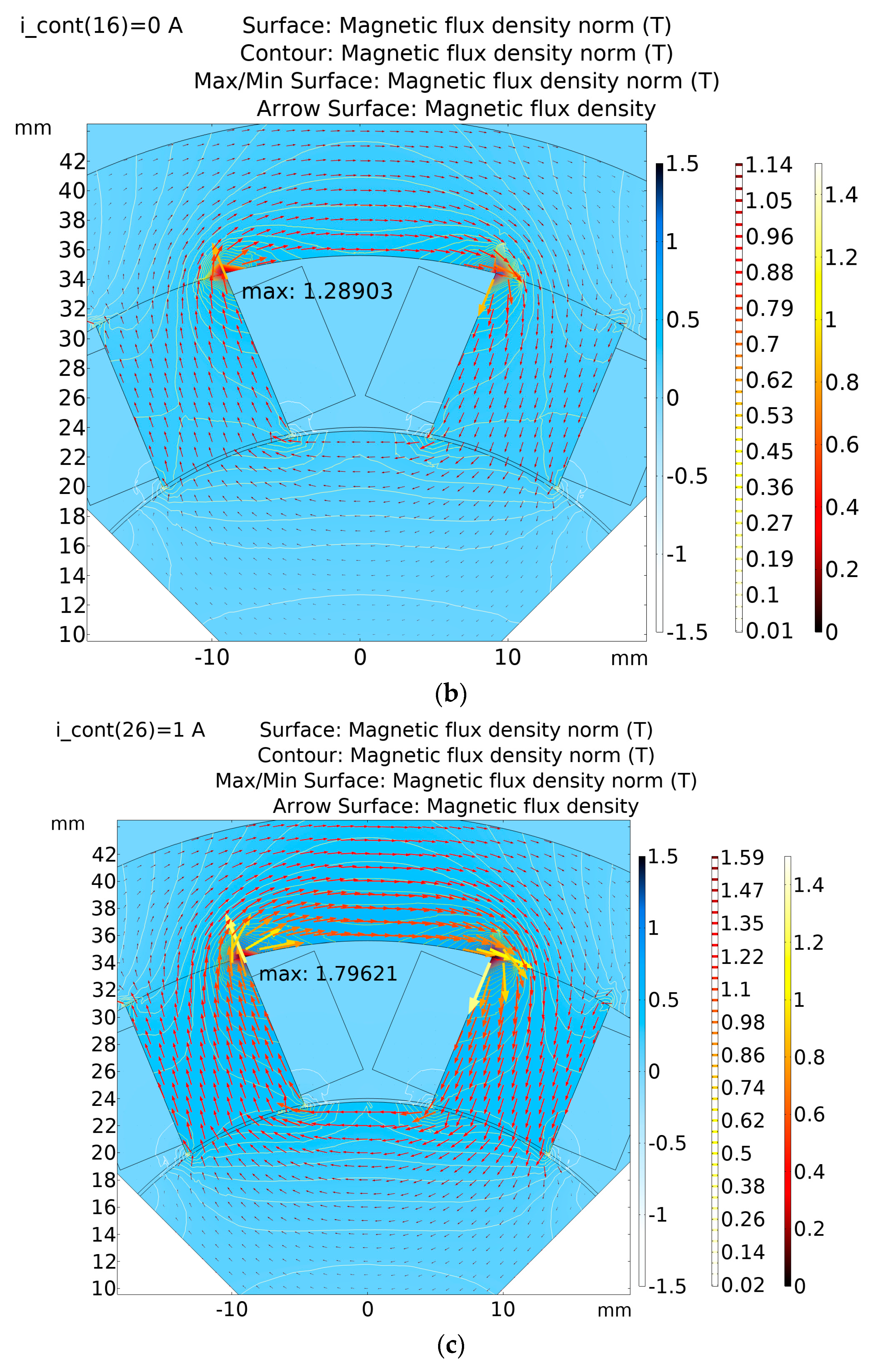
The static characteristics of the rotor–shaft raceway in the air gap for the nominal position are presented in Figure 12a and part (a) of

Table 2. Magnetic forces for different control currents (Figure 12a) (a); magnetic forces for different displacements (Figure 12b) (b).

(a)
Control Current	Force up (Magnetic Force Generated by Upper Electromagnet)	Force Down (Magnetic Force Generated by Bottom Electromagnet)	Resultant Force
−1.5000	0.0000	−56.451	−56.451
−1.4000	0.062211	−52.741	−52.679
−1.3000	0.24884	−49.159	−48.910
−1.2000	0.55991	−45.702	−45.142
−1.1000	0.99546	−42.372	−41.377
−1.0000	1.5556	−39.168	−37.612
−0.90000	2.2409	−36.089	−33.849
−0.80000	3.0518	−33.137	−30.085
−0.70000	3.9884	−30.311	−26.322
−0.60000	5.0502	−27.611	−22.560
−0.50000	6.2378	−25.037	−18.799
−0.40000	7.5510	−22.590	−15.039
−0.30000	8.9898	−20.269	−11.279
−0.20000	10.555	−18.074	−7.5190
−0.10000	12.245	−16.005	−3.7595
0.0000	14.062	−14.062	0.0000
0.10000	16.005	−12.245	3.7595
0.20000	18.074	−10.555	7.5190
0.30000	20.269	−8.9898	11.279
0.40000	22.590	−7.5510	15.039
0.50000	25.037	−6.2378	18.799
0.60000	27.611	−5.0502	22.560
0.70000	30.311	−3.9884	26.322
0.80000	33.137	−3.0518	30.085
0.90000	36.089	−2.2409	33.849
1.0000	39.168	−1.5556	37.612
1.1000	42.372	−0.99546	41.377
1.2000	45.702	−0.55991	45.142
1.3000	49.159	−0.24884	48.910
1.4000	52.741	−0.062211	52.679
1.5000	56.451	0.0000	56.451
(b)
Control Current	Force up (Magnetic Force Generated by Upper Electromagnet)	Force Down (Magnetic Force Generated by Bottom Electromagnet)	Resultant Force
−0.00012000	6.9406	−43.533	−36.592
−0.00010000	7.6708	−34.228	−26.557
−0.000080000	8.5331	−27.642	−19.109
−0.000060000	9.5706	−22.800	−13.229
−0.000050000	10.156	−20.858	−10.702
−0.000040000	10.790	−19.110	−8.3200
−0.000030000	11.491	−17.631	−6.1396
−0.000020000	12.259	−16.321	−4.0617
−0.000010000	13.111	−15.110	−1.9990
0.0000	14.062	−14.062	0.0000
0.000010000	15.110	−13.111	1.9990
0.000020000	16.321	−12.259	4.0617
0.000030000	17.631	−11.491	6.1396
0.000040000	19.110	−10.790	8.3200
0.000050000	20.858	−10.156	10.702
0.000060000	22.800	−9.5706	13.229
0.000080000	27.642	−8.5331	19.109
0.00010000	34.228	−7.6708	26.557
0.00012000	43.533	−6.9406	36.592

. This includes the magnetic distribution of forces generated by the lower electromagnet (force down), the upper electromagnet (force up), and the differential forces (differential forces). The current stiffness of the magnetic bearing can be obtained from this characteristic. The static characteristics for the rotor–shaft raceway displacement of 0.05 and −0.05 mm are shown in Figure 13a,b.

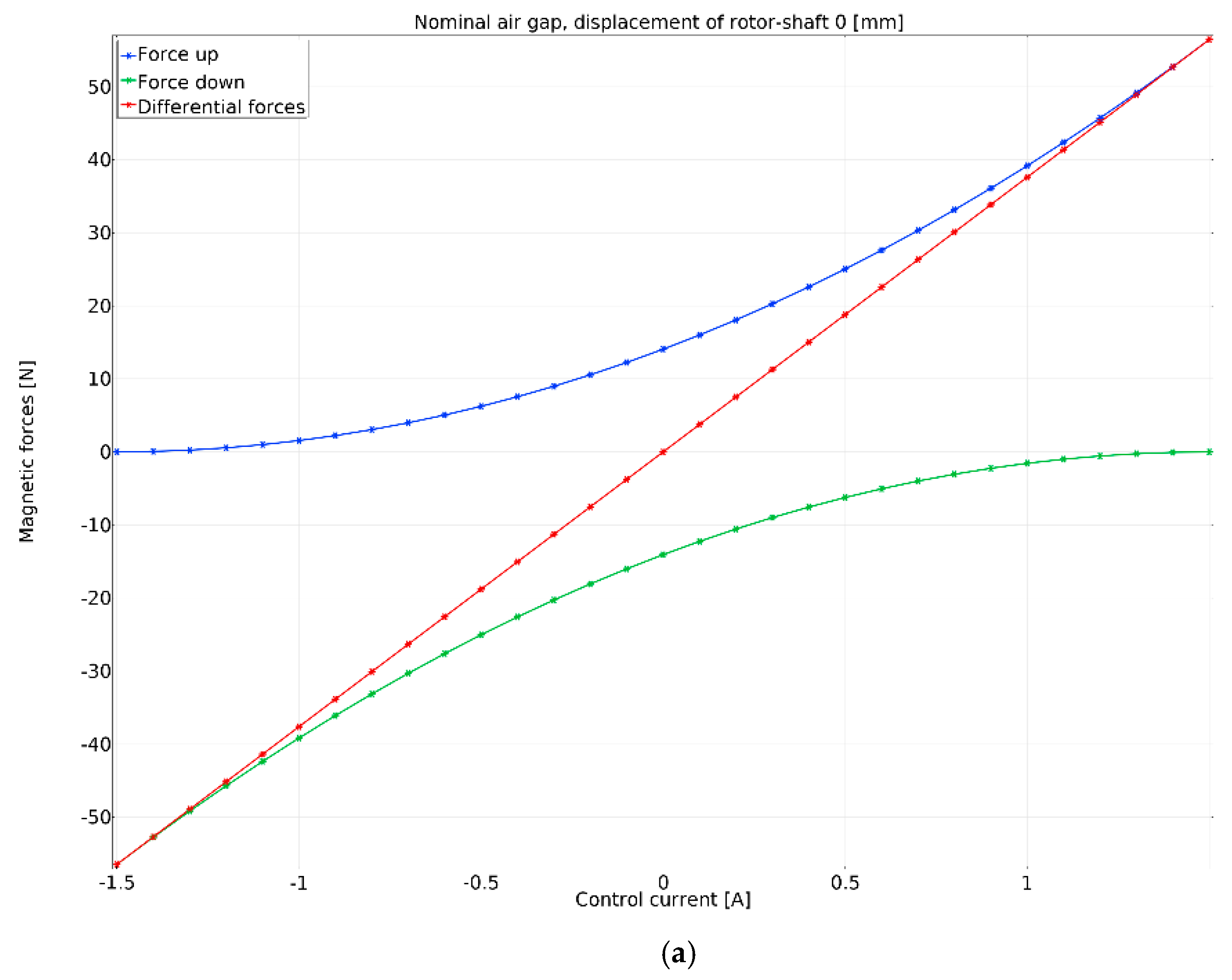
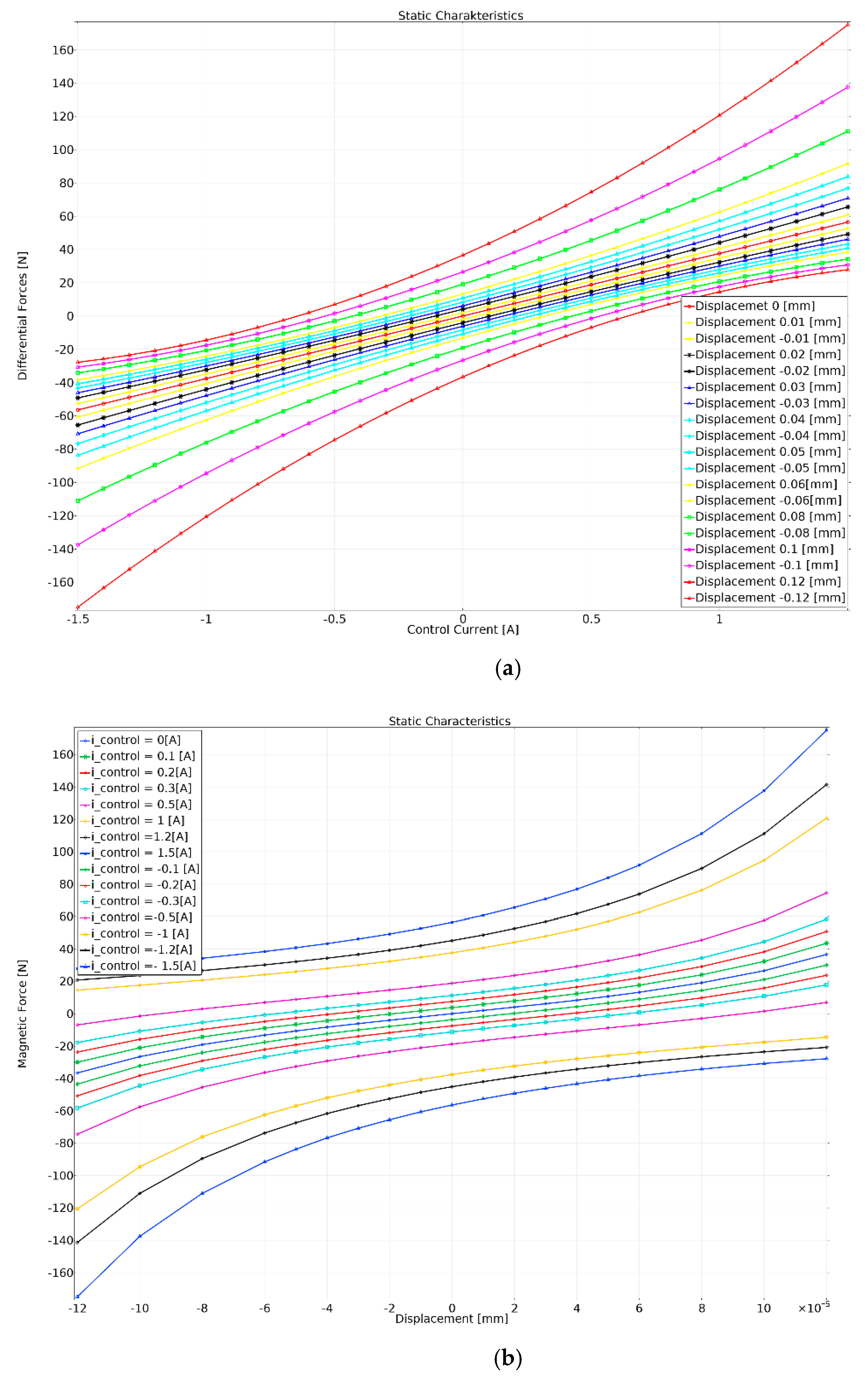
The group of characteristics for the different displacements of the rotor–shaft raceway is presented in Figure 14a. If the displacement is greater than 0.05 mm, the static characteristics lose linearity.

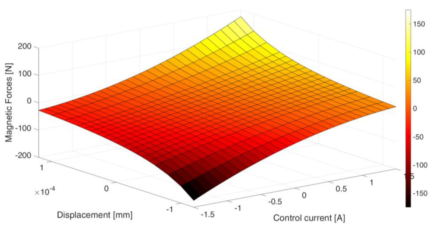
The next group of static characteristics were obtained as a function of the displacement of the rotor–shaft raceway in the air gap for the control current. Those characteristics can be used to estimate the displacement stiffness of the magnetic bearing. The magnetic forces of the current in the operation point are presented in Figure 12b and in part (b) of Table 2. The magnetic forces for the control current of 0.4 A and −0.4 A are shown in Figure 15, and the respective group of the static characteristics is presented in Figure 12b. The linear range of the static characteristics reduces to an interval value from −0.05 to 0.05 mm for this bearing. The magnetic force expressed as a function of the displacement and control current is presented in Figure 16. This characteristic was calculated for the radial magnetic bearing model with the air gap $x_0=0.25$ mm and the operation current $i_0=1.5$ A.

3.2. Experimental Verification

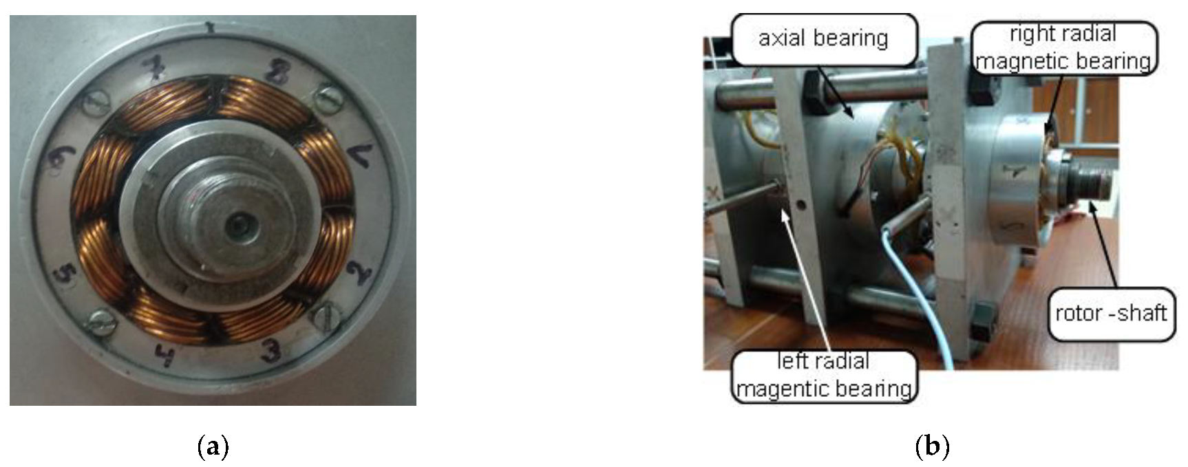
The radial active magnetic bearing shown in Figure 17a was used for the studies performed in this paper. This bearing is part of the magnetic support system of the rotor–shaft, as demonstrated in Figure 17b. The radial magnetic bearings can generate a maximum electromagnetic force of 400 N, and the respective air gap is equal to 0.25 mm. Thus, the operating point current for each bearing is equal to 4 A at the maximum current value of 8 A. The basic parameters of the AMB designed in this paper are shown in Table 1.

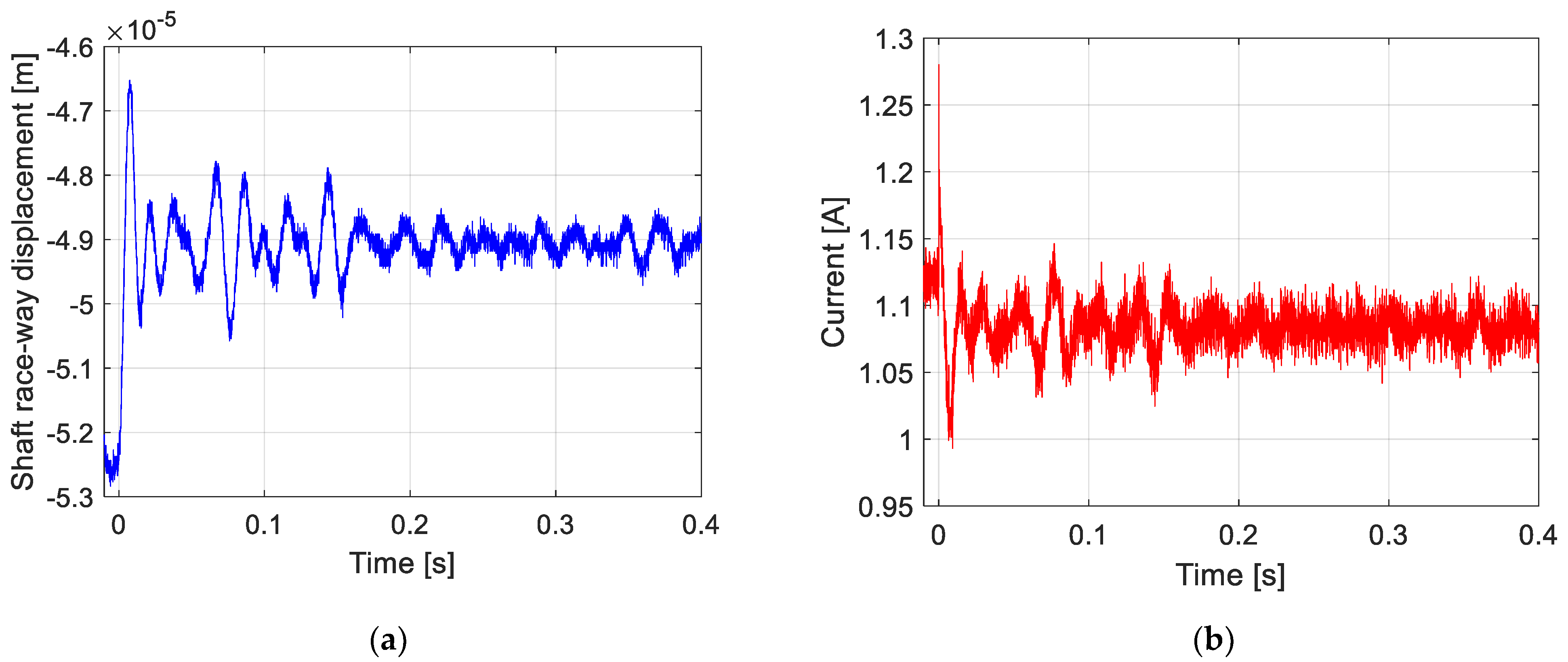
During experimental verification of the generated magnetic forces, time histories of the vertical rotor–shaft raceway displacements in the air gap and the control current were registered for different reference signal values. These courses had the form of a square wave with an amplitude of 0.001, 0.002, 0.005, 0.007, 0.01 V and a frequency of 1 Hz. The registered exemplary time histories are presented in Figure 18.

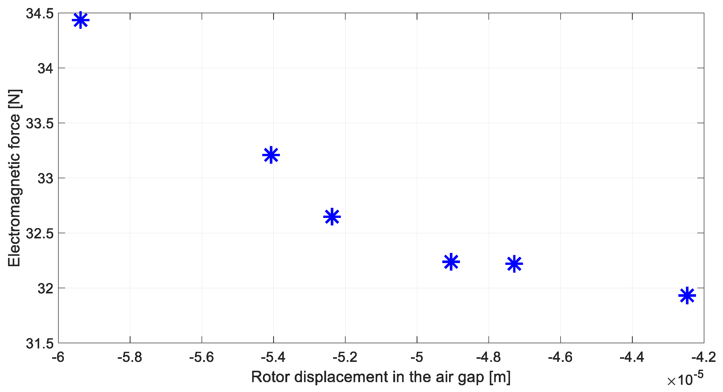
Values of the rotor–shaft raceway displacement x and the control current i in steady-state operating conditions were determined for each data set registered during research experiments. In turn, the electromagnetic force values were obtained based on the analytically calculated displacement stiffness coefficient k_x and current stiffness coefficient k_i, as seen in

Table 3. Current and displacement stiffness coefficient calculated analytically and using Comsol Multiphysics software.

Parameters	Symbol	Value	Unit
Analytical current stiffness	ki	40.6687 for i0 = 1.5 A, x0 = 0.25 mm	N/A
Analytical displacement stiffness	kx	2.4401 × 105 for i0 = 1.5 A, x0 = 0.25 mm	N/m
Current stiffness calculated in Comsol Multiphysics software	ki	37.6152 for i0 = 1.5 A, x0 = 0.25 mm, I = 1.1 A	N/A
Displacement stiffness calculated in Comsol Multiphysics software	kx	2.080 × 105 for i0 = 1.5 A, x0 = 0.25 mm, x = −0.04 mm	N/m
Displacement stiffness calculated in Comsol Multiphysics software	kx	2.205 × 105 for i0 = 1.5 A, x0 = 0.25 mm, x = −0.06 mm	N/m

. All recorded results are listed in

Table 4. Measured parameters of the AMB.

Shaft Raceway Displacement x (m)	Control Current i (A)	Electromagnetic Force F (N)
−0.00004247	1.040	31.9323
−0.00004729	1.076	32.2203
−0.00004905	1.087	32.2382
−0.00005237	1.117	32.6481
−0.00005407	1.141	33.2094
−0.00005938	1.203	34.4351

. In addition, values of the resultant electromagnetic force generated by the magnetic bearing for different displacements of the rotor–shaft raceway are presented in Figure 19.

In the next section of this paper, the experimental investigation results presented in Figure 19 will be compared with the similar results obtained using FEM analysis.

4. Discussion

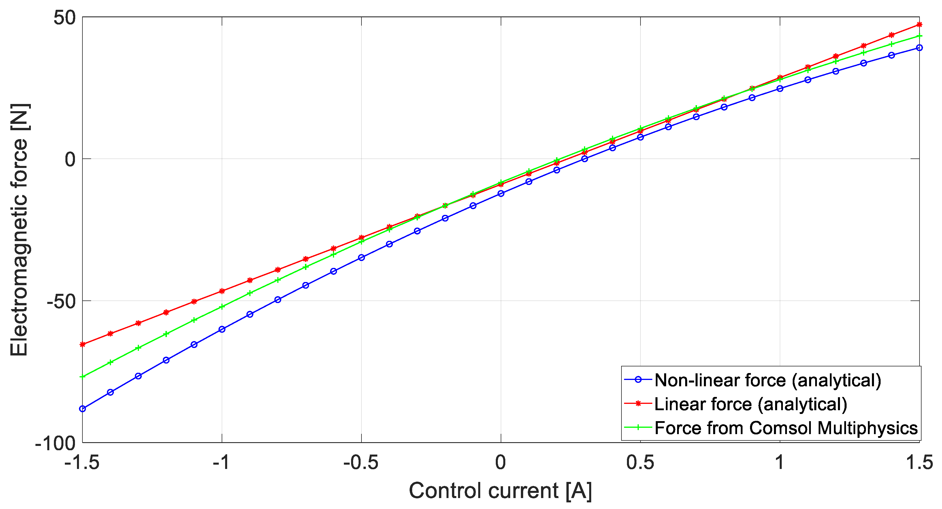
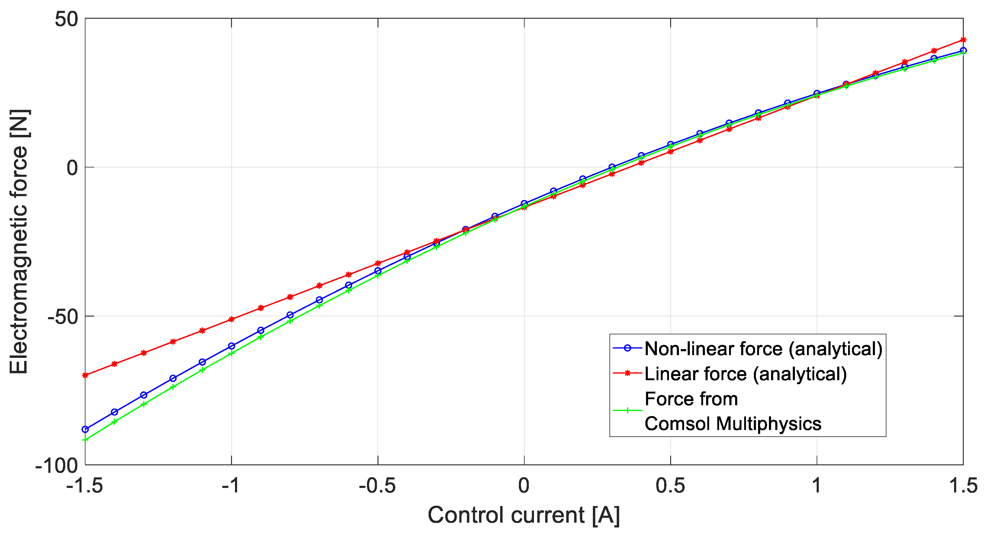
In this paper, theoretical and experimental investigations devoted to determining the electromagnetic force values in a radial bearing were carried out. The resultant electromagnetic force was calculated for various control currents and constant rotor–shaft raceway displacements in the air gap. This force was estimated by expressions (3) and (4). Equation (3) defines the non-linear form of the resultant magnetic force and, using Equation (4), the linear formula of the resultant magnetic force was expressed. After that, the resultant force concerning the electromagnetic force for different control current values and bearing journal positions was modelled using Comsol Multiphysics software. The static characteristics for the displacement of the rotor–shaft raceway in the air gap equal to −0.04 and -0.06 mm are presented in Figure 20 and Figure 21, respectively.

In Figure 20 and Figure 21, the characteristics of the resultant electromagnetic force calculated by the use of non-linear (3) and linear (4) relationships are marked by the blue and red lines, respectively. The characteristics of the resultant electromagnetic force obtained employing Comsol Multiphysics software are illustrated by the green line, which is also presented in Figure 14.

Comparing the characteristics of the resultant electromagnetic force obtained analytically using the non-linear function (3) with the analogous characteristics determined by Comsol Multiphysics software, a high similarity can be observed. For the control current equal to 1.5 A, the maximal disparities had values of 4.16 N and 0.74 N, corresponding accordingly to 9.5% and 2%, respectively, for the characteristics in Figure 20 and Figure 21. In addition, the greatest differences between the characteristics obtained analytically with the use of linear relationship (4) can be noticed for greater values of the control current. This means that the differences increase when moving away from the value of the work point.

Next, the results received theoretically were verified experimentally through the laboratory stand presented in Figure 17. The experimentally registered values of the resultant electromagnetic force were calculated using the measured values of displacement of the rotor–shaft raceway in the air gap and the control currents listed in Table 4 and using the values of displacement and current stiffness coefficients contained in Table 3.

The displacement and current stiffness coefficient values contained in Table 4 were determined using the analytical formulae (5), in which an ideal performance of bearing elements was assumed. Additionally, this table shows the k_x and k_i coefficients based on the characteristics shown in Figure 14 and determined by means of the Comsol Multiphysics software. Therefore, a study of two cases was analyzed. The cases with the resultant electromagnetic force determined based on coefficients k_x and k_i obtained analytically are presented in Figure 22a and Figure 23a. In turn, the variants with the resultant electromagnetic forces determined based on coefficients k_x and k_i determined using the Comsol Multiphysics software are shown in Figure 22b and Figure 23b. Additionally, electromagnetic force values obtained experimentally and theoretically are presented in part (a) and (b) of

Table 5. The resultant electromagnetic forces generated by the magnetic bearing for different control current values for the constant rotor–shaft raceway displacement equal to −0.04 mm and coefficients kx and ki were obtained analytically (a); the resultant electromagnetic forces generated by the magnetic bearing for different values of the control current for the constant rotor–shaft raceway displacement equal to −0.04 mm, where coefficients k_x and k_i were obtained using Control Multiphysics software (b).

(a)
Control Current (A)	Experimental Electromagnetic Force (N)	Theoretical Electromagnetic Force (Comsol Multiphysics) (N)
1.04	32	29.2
1.08	32.2	30.5
1.09	32.2	30.7
1.12	32.6	31.8
1.14	33.2	33.2
(b)
Control current [A]	Experimental electromagnetic force (N)	Theoretical electromagnetic force (Comsol Multiphysics) (N)
1.04	30.3	29.2
1.08	30.6	30.5
1.09	30.7	30.7
1.12	31.1	31.8
1.14	31.7	33.2

, respectively. These parts of Table 5 present a comparison of the theoretical and experimental investigations shown in Figure 22a,b. Similarly, part (a) and (b) of

Table 6. The resultant electromagnetic forces generated by the magnetic bearing for different control current values for the constant rotor–shaft raceway displacement equal to −0.06 mm and coefficients k_x and k_i were obtained analytically (a); the resultant electromagnetic forces generated by the magnetic bearing for different values of the control current for the constant rotor–shaft raceway displacement equal to −0.06 mm; where coefficients k_x and k_i were obtained using Control Multiphysics software (b).

(a)
Control Current (A)	Experimental Electromagnetic Force (N)	Theoretical Electromagnetic Force (Comsol Multiphysics) (N)
1.04	32	25.2
1.08	32.2	26.5
1.09	32.2	27.1
1.12	32.6	27.9
1.14	33.2	28.5
(b)
Control Current (A)	Experimental Electromagnetic Force (N)	Theoretical Electromagnetic Force (Comsol Multiphysics) (N)
1.04	29.8	25.2
1.08	30.0	26.5
1.09	30.1	27.1
1.12	32.6	27.9
1.14	30.5	28.5

present the analogous data from Figure 23a,b.

In Figure 22 and Figure 23, the resultant electromagnetic force characteristics calculated using the non-linear and linear expressions (3) and (4) are marked by blue and red lines, respectively. In turn, the characteristics of the resultant electromagnetic force obtained using the Comsol Multiphysics software are presented by the green line. The colours of these lines correspond to those used in Figure 20 and Figure 21. Additionally, in Figure 22 and Figure 23, the experimental findings of the resultant electromagnetic force are illustrated by the violet and pink markers.

The results presented in Figure 22 and Figure 23 show that a high agreement was obtained between the theoretical and experimental studies. Smaller differences were received for the smaller rotor–shaft raceway displacement, as seen in Figure 22. This result was expected according to the characteristics shown in Figure 14 because, with the increase in the rotor–shaft raceway displacement and value of the current, the non-linearity of the characteristic increases too. Additionally, a greater matching of experimental and theoretical data occurs with the assumption of coefficients k_x and k_i determined by Comsol Multiphysics software, as seen in Figure 22b and Figure 23b.

5. Conclusions

This paper presents the results of theoretical and experimental research on the static characteristics of a radial magnetic bearing intended to support the rotor–shaft in an electric jet engine. The aviation electric jet engine is an innovative technological solution within the increasingly widely used idea of "Electric aircraft". By replacing the gas turbine in this engine with an electric motor, the environment is not adversely burdened with exhaust gases. Moreover, the use of magnetic support for the entire rotating system allows the provision of much better operating properties than the rolling bearings traditionally used for this purpose. No friction or lubrication means are needed to characterize active magnetic bearings because of the lack of mechanical contact between operation elements, the low amplitude level of lateral rotor vibrations, their high durability, and their long-term high-speed running ability. These features give the magnetic bearings a considerable potential to become a key element in rotating machines such as jet engines. Therefore, this work focuses on a thorough study of the load-bearing properties of an active magnetic bearing. In particular, the values of the electromagnetic forces were determined in a theoretical and experimental way.

The main goal of this research was to verify a non-parametric numerical model of the active magnetic bearing. Having a verified model allows the design of complex magnetic bearings for different applications. The 3D model of the bearing allows observation of the magnetic phenomena and inside processes such as:

• The distribution of magnetic flux density in the magnetic circuit of the magnetic bearing (the steal and an air gap);
• The distribution of the magnetic field;
• The distribution of the neglected magnetic field;
• Magnetisation;
• The density of the electric current;
• The density of the induced current;
• The magnetic notch phenomenon;
• The influence of control current and the position of the rotor in the air gap for magnetic forces.

There were obtained experimental results that can be used to verify this numerical model of an active magnetic bearing. The model was made using FEM analysis in Comsol Multiphysics software. The model of the magnetic bearing was verified by comparing the results of the tests and the results of the simulations (the static characteristics). The verified model and verified methodology of modelling can be used to optimise the active magnetic bearing dedicated for rotation machines, especially for jet engines. The numerical test significantly speeds up the process design of the active magnetic bearing.

The paper also presents the results of experimental tests using an experimental stand in the form of a rotor shaft supported by two magnetic radial bearings and one axial bearing to verify the theoretical calculations’ findings. During these tests, there were recorded displacements of the rotor–shaft raceway in the air gap, and the steady-state control current, registered as employing the control system with the PD regulator. On this basis, the resultant electromagnetic force of the bearing reaction was calculated.

The values of the resultant electromagnetic force obtained on the basis of the results of the experimental tests were determined for two cases: using the combination of the analytically calculated k_x and k_i coefficient values, and by means of the Comsol Multiphysics software. It turned out that both approaches led to the high mutual similarity of the results, but their greater discrepancy was observed with the use of the Comsol Multiphysics software than with the analytically calculated ones. In addition, smaller differences in the values of the theoretically and experimentally determined forces occurred with a smaller shift of the rotor–shaft raceway in the air gap.

Finally, it should be stated that, in this work, the experimental validation of theoretical models of the active magnetic bearing was carried out. Analysis and comparisons between theoretical and experimental results showed that models prepared using Comsol Multiphysics software are proper and well defined. These models can be used for further qualitative analyses and the design of various structures and configurations of the bearing arrangement intended for use in an electric jet engine. In the next step of research in this field, an analogous approach will be applied to the magnetic active axial bearing and the radial passive magnetic bearings.

All in all, such an innovative concept of an aircraft engine requires a lot of further research. Thus, the investigation results described in this paper should be treated as very fundamental. Regardless of the natural need to consider numerous material, thermal, and technological problems, among others, an extremely important aspect is the issue of the dynamic interaction of the rotating system of an electric jet engine with its housing, where the magnetic support properties play an extremely important role. Therefore, each of these four variants of the bearing support of the rotor shaft and the motor presented at the beginning of this work require a detailed dynamic analysis of their shaft-bearing housing systems to predict an adequately stable and endurance-safe operation. Additionally, investigations into the effective control of the operation of the compressor rotor drive, employing the electric motor in various conditions to ensure the required thrust, should be carried out.

References

- Botten, S.L.; Whitley, C.; King, A.D. Flight control actuation Technology for next-generation all-electric aircraft. Technol. Rev. J. 2000, 8, 55–68. [Google Scholar]
- Kozakiewicz, A.; Grzegorczyk, T. Electric Aircraft Propulsion. J. KONBiN 2021, 51, 49–66. [Google Scholar] [CrossRef]
- Saucedo-Dorantes, J.J.; Arellano-Espitia, F.; Delgado-Prieto, M.; Osornio-Rios, R.A. Diagnosis methodology based on deep feature learning for fault identification in metallic, hybrid and ceramic bearings. Sensors 2021, 21, 5832. [Google Scholar] [CrossRef] [PubMed]
- Gosiewski, Z.; Henzel, M.; Falkowski, K.; Żokowski, M. Numerical and Experimental Testing of Bearingless Induction Motor. Solid State Phenom. 2013, 198, 382–387. [Google Scholar] [CrossRef]
- Chiba, A.; Fukao, T.; Ichikawa, O.; Oshima, M.; Takemoto, M.; Dorrell, D. Magnetic Bearings and Bearingless Drives; Elsevier’s Science Technology Rights Department in Oxford: Oxford, UK, 2005; pp. 1–96. [Google Scholar]
- Sandtner, J.; Bleuler, H. Electrodynamic Passive Magnetic Bearing with Planar Halbach Arrays. In Proceedings of the 9th Int. Symposium on Magnetic Bearings, Lexington, KY, USA, 3–6 August 2004. [Google Scholar]
- Falkowski, K. The ring with molecular current as the model of the passive magnetic bearing. J. Vibroengineering 2012, 14, 135–142. [Google Scholar]
- Sun, X.; Su, B.; Chen, L.; Yang, Z.; Li, K. Design and analysis of interior composite-rotor bearingless permanent magnet synchronous motors with two layer permanent magnets. Bull. Pol. Acad. Sci. Tech. Sci. 2017, 65, 833–843. [Google Scholar] [CrossRef]
- ISO14839-1; “Mechanical Vibration—Vibration of Rotating Machinery Equipped with Active Magnetic Bearings”—Part 1: Vocabulary. 2nd ed. 2018. Available online: https://www.iso.org/standard/68127.html (accessed on 30 October 2018).
- Filatov, A.V.; Maslen, E.H.; Gillies, G.T. A method of non-contact suspension of rotating bodies using electromagnetic forces. J. Appl. Phys. 2002, 91, 2355–2371. [Google Scholar] [CrossRef]
- Filatov, A.V.; Maslen, E.H.; Gillies, G.T. Stability of an electro-dynamic suspension. J. Appl. Phys. 2002, 92, 3345–3353. [Google Scholar] [CrossRef]
- Lembke, T.A. Design and Analysis of a Novel Low Loss Homopolar Electro-Dynamic Bearing. Ph.D. Thesis, KTH Electrical Engineering, Stockholm, Sweden, 2005. [Google Scholar]
- Amati, N.; De Lépine, X.; Tonoli, A. Modeling of electro-dynamic bearings. ASME J. Vib. Acoust. 2008, 130, 061007–061016. [Google Scholar] [CrossRef]
- Detoni, J.G.; Impinna, F.; Tonoli, A.; Amati, N. Unified modeling of passive homopolar and heteropolar electro-dynamic bearings. J. Sound Vib. 2012, 331, 4219–4232. [Google Scholar] [CrossRef]
- Cui, P.; He, J.; Fang, J.; Xu, X.; Cui, J.; Yang, S. Research on method for adaptive imbalance vibration control for rotor of variable-speed mscmg with active-passive magnetic bearings. J. Vib. Control. 2015, 23, 167–180. [Google Scholar] [CrossRef]
- Impinna, F.; Detoni, J.G.; Tonoli, A.; Amati, N.; Piccolo, M.P. Test and Theory of Electro-Dynamic Bearings Coupled to Active Magnetic Dampers. In Proceedings of the 14th Int. Symposium on Magnetic Bearings, Linz, Austria, 11–14 August 2014. [Google Scholar]
- Cui, Q. Stabilization of Electrodynamic Bearings with Active Magnetic Dampers. Ph.D. Thesis, No. 7334. École Polytechnique Fédérale de Lausanne, Lausanne, Switzerland, 2016. [Google Scholar]
- Detoni, J.G.; Impinna, F.; Amati, N.; Tonoli, A.; Piccolo, M.P.; Genta, G. Stability of a 4 Degree of Freedom Rotor on Electro-Dynamic Passive Magnetic Bearings. In Proceedings of the 14th Int. Symposium on Magnetic Bearings, Linz, Austria, 11–14 August 2014. [Google Scholar]
- Szolc, T.; Falkowski, K.; Henzel, M.; Kurnyta-Mazurek, P. The determination of parameters for a design of the stable electro-dynamic passive magnetic support of a high-speed flexible rotor. Bull. Pol. Acad. Sci. Tech. Sci. 2019, 67, 91–105. [Google Scholar]
- Szolc, T.; Falkowski, K.; Kurnyta-Mazurek, P. Design of a combined self-stabilizing electro-dynamic passive magnetic bearing support for the automotive turbocharger rotor. J. Vib. Control. 2020, 27, 815–826. [Google Scholar] [CrossRef]
- Carvalho Souza, F.E.; Silva, W.; Ortiz Salazar, A.; Paiva, J.; Moura, D.; Villarreal, E.R.L. A Novel Driving Scheme for Three-Phase Bearingless Induction Machine with Split Winding. Energies 2021, 14, 4930. [Google Scholar] [CrossRef]
- Chen, Y.; Bu, W.; Qiao, Y. Research on the Speed Sliding Mode Observation Method of a Bearingless Induction Motor. Energies 2021, 14, 864. [Google Scholar] [CrossRef]
- Hua, Y.; Zhu, H.; Gao, M.; Ji, Z. Design and Analysis of Two Permanent-Magnet-Assisted Bearingless Synchronous Reluctance Motors with Different Rotor Structure. Energies 2021, 14, 879. [Google Scholar] [CrossRef]
- Wang, X.; Zhang, Y.; Gao, P. Design and Analysis of Second-Order Sliding Mode Controller for Active Magnetic Bearing. Energies 2020, 13, 5965. [Google Scholar] [CrossRef]
Figure 1.
Concepts of the electric jet engine: configurations of jet engines with radial and axial active magnetic bearings and with a bearingless drive (a); configurations of a jet engine with one passive radial magnetic bearing, one axial active magnetic bearing and with a bearingless drive (b).
Figure 2.
Active magnetic suspension: rotor in the operation point (a), rotor outside of the operation point (b).
Figure 3.
The geometrical shapes of the radial magnetic bearing components—magnetic circuits (a) air zones in the model (b).
Figure 4.
Electromagnetic actuators of the radial electromagnetic bearing—the armature of the actuator (a) and the rotor as an element of the actuator (b); reduced model of the radial electromagnetic bearing (c).
Figure 5.
The magnetisation curve of silicon steel Et140-30.
Figure 6.
The mesh air gap (a), steel ET 140-30 (b), and coils of the electromagnet (c).
Figure 7.
Current density for the control current −1 A (a), 0 A (b), and 1 A (c).
Figure 8.
Streamline magnetic flux density for the control current of −1 A (a), 0 A (b), and 1 A (c).
Figure 9.
Magnetic flux density for the control current of −1 A (a), 0 A (b), and 1 A (c).
Figure 10.
Magnetic flux density along the magnetic bearing for a control current of 0 A (a) and 1.5 A (b).
Figure 11.
Distribution of magnetic flux density of (a) the magnetic field and (b) along the radial bearing for the control current.
Figure 12.
Magnetic forces for the nominal position of the shaft raceway in the air gap (a) and the current of the working point (b).
Figure 13.
Magnetic forces vs. displacements of the rotor–shaft raceway equal to 0.05 mm (a) and −0.05 mm (b).
Figure 14.
The static characteristics for different displacements of the rotorshaft raceway in the air gap (a) and various control currents (b).
Figure 15.
Magnetic forces for the control current of -0.4 A (a) and 0.4 A (b).
Figure 16.
Magnetic force as a function of displacement of the rotor–shaft raceway in the air gap and control current.
Figure 17.
Laboratory object: (a) radial active magnetic bearing; (b) rotor–shaft support system.
Figure 18.
Time histories of the registered quantities: the rotor–shaft raceway displacement (a); the control current (b).
Figure 19.
The resultant electromagnetic force generated by the magnetic bearing for different displacements of the rotor–shaft raceway.
Figure 20.
The resultant electromagnetic force generated by the magnetic bearing for different values of the control current for the rotor–shaft raceway displacement is equal to −0.04 mm.
Figure 21.
The resultant electromagnetic force generated by the magnetic bearing for different values of the control current for the rotor–shaft raceway displacement is equal to −0.06 mm.
Figure 22.
The resultant electromagnetic forces generated by the magnetic bearing for different values of the control current for the constant rotor–shaft raceway displacement equal to −0.04 mm with experimental results: coefficients kx and ki obtained analytically (a); coefficients kx and ki determined with the use of Comsol Multiphysics software (b).
Figure 23.
The resultant electromagnetic forces generated by the magnetic bearing for different values of the control current for the constant rotor–shaft raceway displacement equal to −0.06 mm with experimental results: coefficients kx and ki obtained analytically (a); coefficients kx and ki determined with the use of Comsol Multiphysics software (b).