Energy Consumption Forecasting in a University Office by Artificial Intelligence Techniques: An Analysis of the Exogenous Data Effect on the Modeling

Abstract

The forecasting of building energy consumption remains a challenging task because of the intricate management of the relevant parameters that can influence the performance of models. Due to the powerful capability of artificial intelligence (AI) in forecasting problems, it is deemed to be highly effective in this domain. However, achieving accurate predictions requires the extraction of meaningful historical knowledge from various features. Given that the exogenous data may affect the energy consumption forecasting model’s accuracy, we propose an approach to study the importance of data and selecting optimum time lags to obtain a high-performance machine learning-based model, while reducing its complexity. Regarding energy consumption forecasting, multilayer perceptron-based nonlinear autoregressive with exogenous inputs (NARX), long short-term memory (LSTM), gated recurrent unit (GRU), decision tree, and XGboost models are utilized. The best model performance is achieved by LSTM and GRU with a root mean square error of 0.23. An analysis by the Diebold–Mariano method is also presented, to compare the prediction accuracy of the models. In order to measure the association of feature data on modeling, the “model reliance” method is implemented. The proposed approach shows promising results to obtain a well-performing model. The obtained results are qualitatively reported and discussed.

1. Introduction

Currently, climate change and natural resource shortages have become significant issues. According to the research of Gaya Herrington [1], resources will run out in a few decades if the consumption rate remains stable. France has been involved internationally in combating climate change with the multiannual energy plan (MAEP), which was published on 25 January 2019 [2]. Residential and industrial buildings are the highest consuming sectors in France, with a share of almost 44% of the total final energy consumption [2,3]. Hence, there are substantial investments to accelerate the transition from traditional to smart buildings. Smart buildings have remarkable resource management and control capabilities. The ability of future smart buildings to forecast energy consumption not only can enhance the energy consumption optimization in buildings, but also, at a higher level, can play a vital role in planning the energy demand response in smart grids. Artificial intelligence techniques are widely used in this domain, and they show their powerful influence, though there remains a wide range of studies to be performed to advance in this investigation area. One of the study areas that needs more attention, and for which there is still a shortage of work, is the importance of feature data and the role they can play to obtain not only an accurate model, but also efficient model construction. The investigation of this area is always complicated due to the unclear participation of various data that can improve or deteriorate the model performance. Having a clear idea of this subject can enhance the model performance and decrease its computation cost. Due to the abovementioned factors, in this investigation, we would like to dig deeper into energy consumption forecasting and study the influence of different data features.

Building load forecasting essentially falls into three categories: short-term forecasts (an hour to one week), medium-term forecasts (a week to a year), and long-term forecasts (longer than a year). Knowing that the majority of building energy data incorporates time-dependent components, recurrent neural networks (RNNs) can usually dissect the building’s energy data directly, and learn the historical information by themselves. The most popular RNN model is the long short-term memory network (LSTM), whereas the use of nonlinear autoregressive models with exogenous inputs (NARX) also show their performance in several important applications [4]. The authors of [5] applied RNN models to forecast the heating load for various buildings within a university campus. Their study suggested that the RNN models have the potential to perform better than feedforward neural network models for medium- to long-term forecasts. However, the study has underlying limitations, as the role of the features is not clear in the learning process. In 2020, Xue et al. compared different ML algorithms to forecast the heating demand of a district system [6]. Their experiment demonstrated that the LSTM models usually obtained higher accuracy than the other data-driven models. The authors selected the features for the training phase based on several methods, such as autocorrelation; however, as methods such as autocorrelation are linear, the role of the features in the construction of a nonlinear model remains questionable. According to a review published in [7], the major factors that affect energy consumption are climate, building system, occupants, and socioeconomic characteristics. Although the studies identified a set of five main categories and other sub-factors affecting building energy consumption, the subfactors can be a major factor, depending on the case study. There is much investigation in this area, and the studies mainly focus on implementing different algorithms, comparing them, and examining the time horizon prediction. The research works of [8,9] are some examples that focus on using deep learning techniques. The work of [10] focuses on forecasting in different time horizons, while also comparing several learning algorithms. It is an interesting study that presents the performance of different learning algorithms in various time horizons; however, it also has leakage regarding the proper protocols for time lag selection and the analysis of input features to the model.

In an investigation by [11], the activity of occupancy data and its influence on ambient data were considered for better prediction of load forecasting in a building. The approach is divided into two directions. In the first direction, the data are separated into nonworking and working hours in order to reduce the effect of occupant activities. In the second direction, an artificial neural network and fuzzy logic are used to predict not only the energy consumption, but also the level of the occupant rates. The obtained results show the performance of the model is improved by 35% and 42% regarding the two approaches, respectively. Their analysis shows the correlation between ambient condition data and energy consumption due to occupant rates, which is a key factor in the prediction model. Despite the novelty of their work in dealing with the challenges of considering different scenarios regarding the occupant rates, the work suffers from a lack of historical data lags as an input to the model. Indeed, the authors were attentive only to ambient data with a regression algorithm, and considered the occupant rates for the prediction. In [12], the authors made an effort to predict the energy consumption of a lighting system based on a support vector machine (SVM)-based approach. They considered daily sky coverage and day type in the modeling of an office building. They used only the SVM and ambient data for constructing the model. However, the effect of ambient data on modeling, which is the prediction of the lighting load, is questionable. This is apart from taking into consideration the time delays of the data, which can be a weakness in such research.

Opposite to the two last investigations, the authors of [13], by keeping in mind the weather data for the energy consumption prediction, used LSTM, support vector regression (SVR), and Gaussian process regression (GPR). Additionally, they considered an analysis of finding important features by the Shapley additive explanation (SHAP) method. The proposed research is interesting, as they presented different algorithms to face the problem, and also paid attention to the effect of important features that can lead to less complex models. They finally made a conclusion that LSTM performed better compared to other examined algorithms. Although, time delay analysis on the dataset is not provided in this work, despite the important role that it plays in algorithms such as LSTM.

The investigation by [14] is focused on using deep neural networks to predict energy consumption, using LSTM, GRU, and drop-GRU for different time horizons. They note that the purpose of their work is to compare which algorithm will come up with better prediction results. After data processing, analyzing, and implementing feature selection, they constructed the models. The hyperparameters were set based on trial and error. Finally, to compare the models, they used RMSE, MAE, R², and time of computation as the metrics. They conclude that GRE, compared to LSTM and drop-GRU, has a better ability to predict while needing fewer hyperparameters to set, and has a simpler architecture compared to the other two. In the work of [15], the electricity consumption forecast of high-rise office buildings is taken into account. The authors used LSTM as the implemented algorithm. They believed the electricity consumption prediction of lighting systems is easier than air conditioners. Due to this fact, they used relative humidity and scheduling as exogenous inputs to improve the accuracy of the model. They also used a backpropagation algorithm, and ARIMA to compare their results. The authors finally, by comparing the results of the three presented algorithms, show the superior performance of LSTM. They noted a high prediction accuracy in the case of lighting electricity consumption, while for the air conditioning electricity consumption prediction, the relative humidity and scheduling data slightly improved the LSTM performance. In the two recent works, despite the efforts of authors to propose an accurate model for predicting, they never considered the optimized number of time lags for prediction. In addition, despite the work of [15] that considered several features as input to improve the performance of the model, the role of features in the training phase was clearly not examined.

In all of the above investigations, despite huge efforts to improve the performance of the model with different model tuning, various data inputs, etc., and examining several algorithms, the majority of them suffer from not enough work illustrating the role of features in modeling performance. More importantly, the configuration of time lags for prediction can greatly affect the complexity of the model, consequently affecting the model’s performance and computational costs. However, this is not studied precisely in a clear framework. Mainly, in favor of feature selection and, also, the setting of time lags, they fulfilled their investigations with empirical or simple data analysis, such as autocorrelation. The objective of this investigation is to deeply analyze the influence of exogenous data and optimized time lags on energy consumption forecasting in buildings within a structured framework by data-driven techniques before and, moreover, after modeling. To that end, this study illustrates the effective methods for modeling energy consumption forecasting in several steps.

The rest of this paper will contribute as follows: Section 2 presents the methodology and the protocols of the implementation, Section 3 introduces the dataset, Section 4 depicts the experimentation, results, and discussion, and finally, Section 5 concludes the investigation and presents the future work.

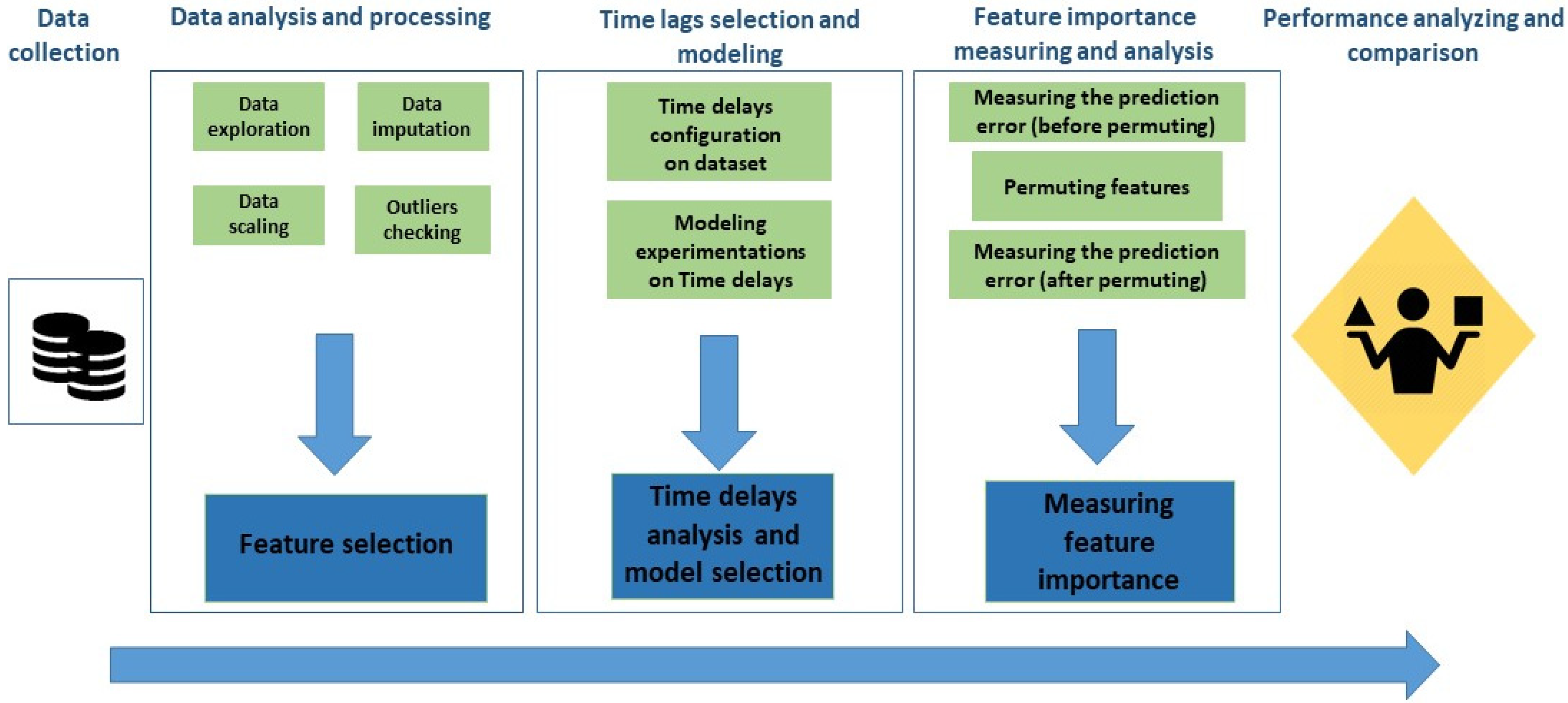
2. Methods and Protocols

In this section, the approach and methods that are utilized in this research work are presented. The schema of the considered protocol for advancing the proposed research idea is illustrated in Figure 1. It is divided into 5 parts: The first part is the data collection to form the needed dataset. In the case of this research work, an open-access dataset is utilized, which is explained in Section 3. The second part is regarding the representation of the raw data, which is followed by data analysis and processing. In this part, the raw data will be prepared for the training process. As shown in the figure, several processes, such as data imputation and scaling of data, are included in this section. The third part is leading to the construction of machine learning models according to different algorithms and input features. The optimum time lags are realized in this part of the study, based on a protocol that is presented in Section 4 of this article. The fourth part illustrates the important inputs and their roles in the learning process of the model based on error measurement and permutation of data features in a defined framework, which is explained comprehensively. Finally, the last part presents the results of the work for analysis, comparison, and discussion. In the next Section 2.1 and Section 2.2, the utilized materials and techniques for conducting the research are presented.

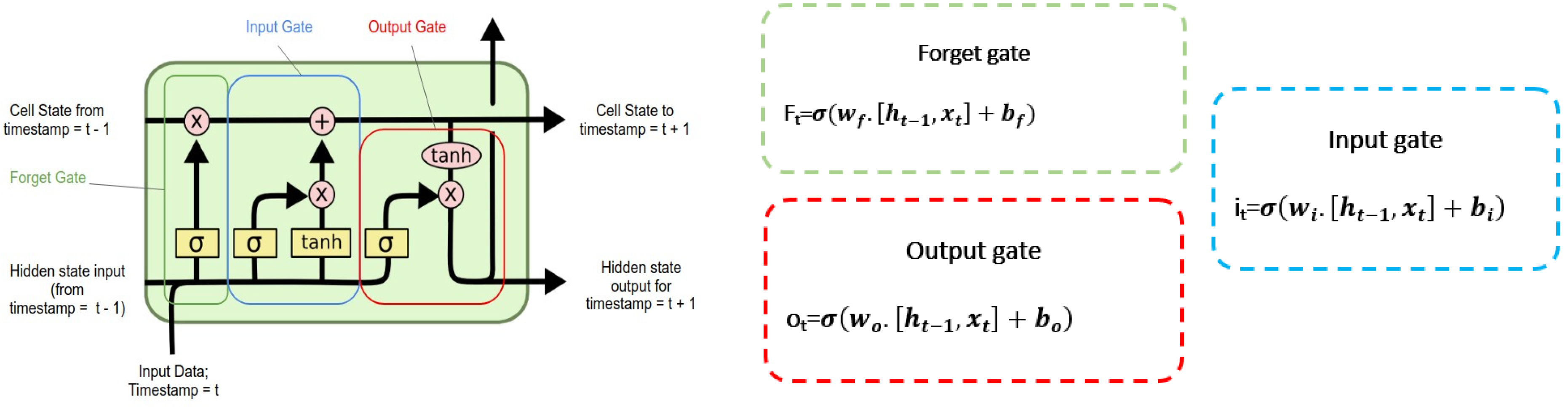
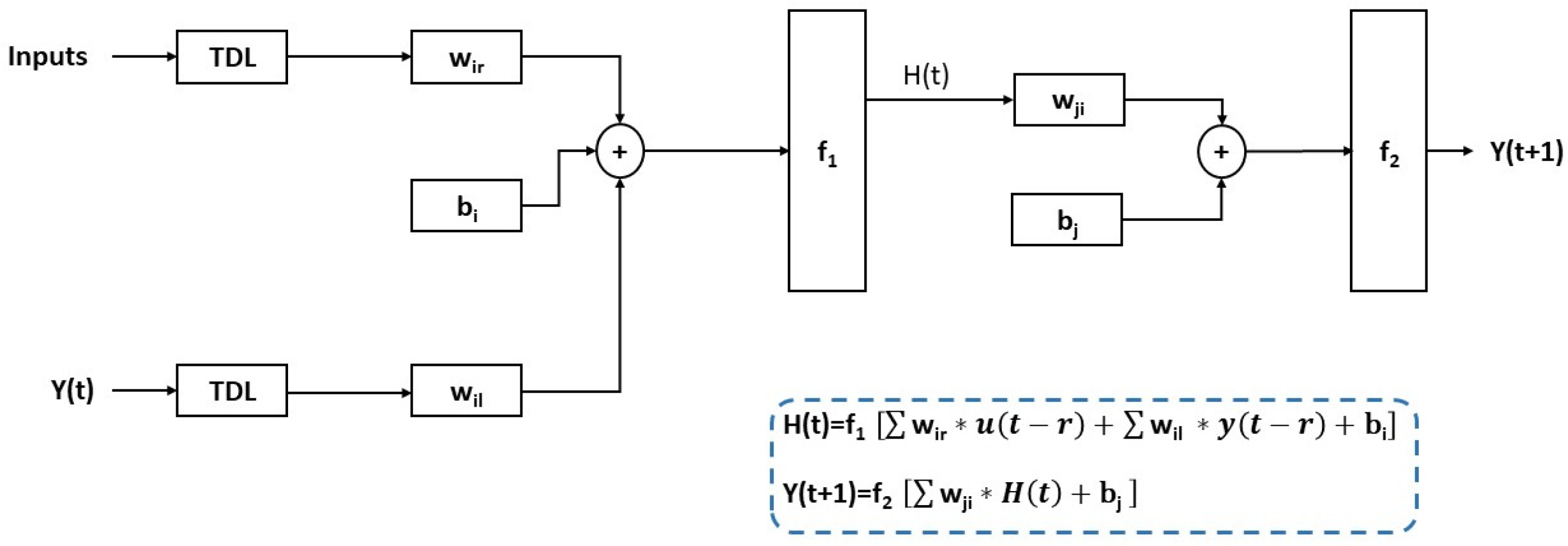
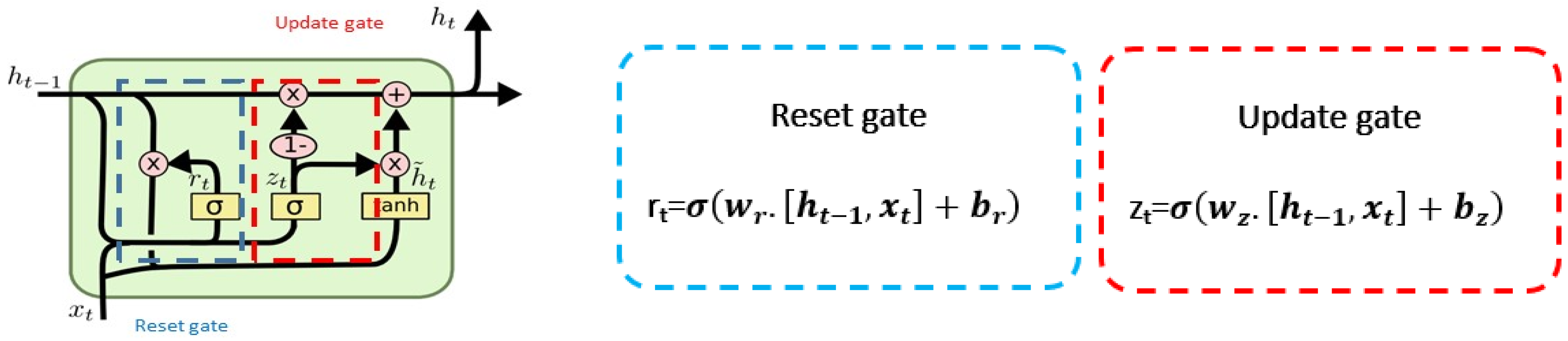
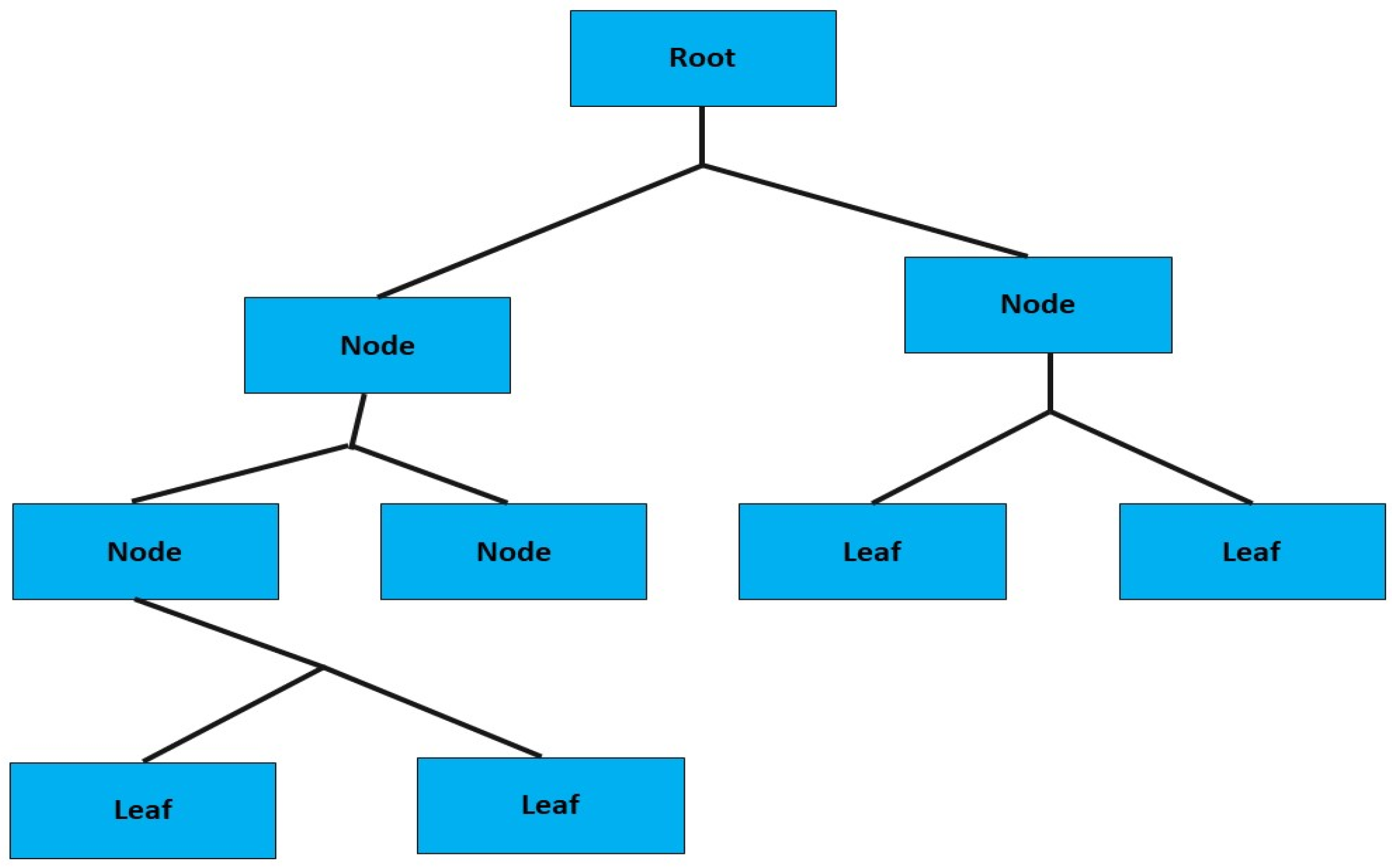
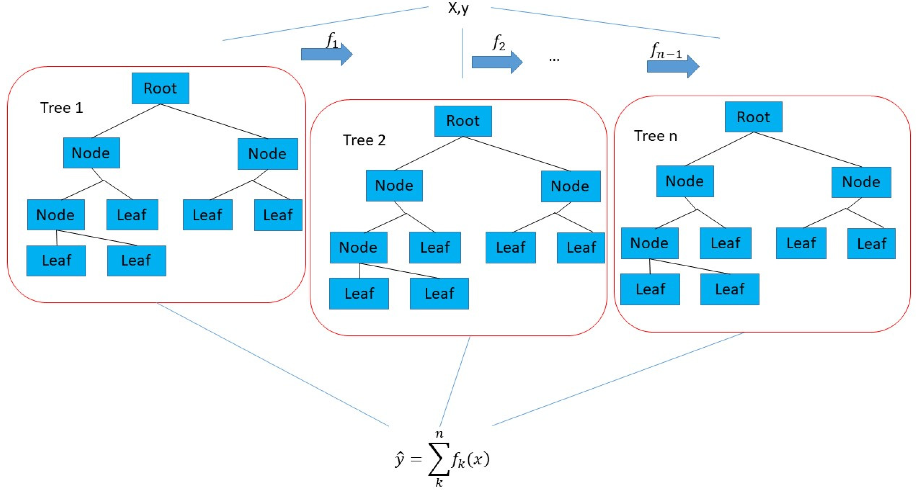
2.1. Machine Learning Algorithms for Modeling Energy Consumption Forecaster

The methodological approach of this research is based on data-driven energy consumption forecasting. Due to the effectiveness of machine learning methods in mimicking complicated time series patterns, LSTM, NARX-MLP, GRU, decision tree, and XGboost are applied.

LSTM is a widely used recurrent neural network in time series forecasting. Its performance in solving time series problems is remarked upon in several works [14,16,17]. LSTM neural networks achieve temporal dependency using special units called memory blocks, which is the main difference between RNNs and ANNs. LSTM is an improved form of RNNs that is capable of overcoming the vanishing gradient problem [18]. The information is passed through a mechanism known as cell states, with three gates to update the previous hidden state. Figure 2 shows the gates and architecture of LSTM [19], where, W_f, W_o, and W_i are the weight matrices, and b_f, b_o, and b_i are the bias vectors. X_t is the current input. h_t and h_t−1 are the output at the current time t and the previous time t₋1, respectively. Finally, σ represents the sigmoid function.

Similarly to LSTM, the nonlinear autoregressive with exogenous (external) inputs (NARX) model predicts series y(t) given past values of series y and another external series u(t). NARX is a specific class of RNN that is widely implemented in various applications [20,21]. NARX can be based on different internal network architectures as a training rule. Figure 3 shows the architecture of NARX, where, TDL is the tapped delayed line, W_ir and W_il are the weights, b_i and b_j are the biases, and f₁ and f₂ are the activation functions.

A time series is a sequence of vectors $\mathrm{u}\left(\mathrm{t}\right), \mathrm{t}=0,1,2,\dots$ where, t represents elapsed time and u is a parameter such as temperature, humidity, etc., which varies with time.

Gated recurrent unit (GRU) is an algorithm which is effective in time series prediction. GRU and LSTM have similar architectures; however, GRU has one less gate, and generally has a simpler architecture than LSTM, though its effectiveness in finding sequential data is undeniable. Figure 4 shows the architecture of GRU and its gates formula, where, h_t is the hidden layer vector, x_t is the input layer vector, b_r and b_z are the bias vectors, w_z and w_r are the weight matrices, and σ represents the sigmoid activation function.

Hence, choosing the ideal tapped delayed line (TDL) or time delay for each feature is crucial for the model’s predictive accuracy. Forecasting time series with neural networks consists of finding a function f to obtain an estimate of y at time t + 1, from N past time steps, so that:

$$\mathrm{y}\left(\mathrm{t} +1\right)=\mathrm{f}\left(\mathrm{y}\left(\mathrm{t}\right),\dots ,\mathrm{y}\left(\mathrm{t}-{\mathrm{n}}_{\mathrm{y}}\right),\mathrm{u}\left(\mathrm{t}\right),\dots ,\mathrm{u}\left(\mathrm{t}-\mathrm{n}{)}_{\mathrm{x}}\right)\right)$$

(1)

where, $\mathrm{u}\left(\mathrm{t}\right),\dots ,\mathrm{u}\left(\mathrm{t}-{\mathrm{n}}_{\mathrm{x}}\right)$ are the present and delayed exogenous inputs, respectively, $\mathrm{y}\left(\mathrm{t}\right),\dots ,\mathrm{y}\left(\mathrm{t}-{\mathrm{n}}_{\mathrm{y}}\right)$ are historical data of $\mathrm{y}\left(\mathrm{t} +1\right)$, and f is the function that computes $\mathrm{y}\left(\mathrm{t} +1\right)$ based on historical exogenous and nonexogenous data. The ideal combination of features chosen in the final model differs from one dataset to another. Therefore, a quantitative and correlation analysis will determine the model’s input. The predictive model aims to predict the final energy consumption one step ahead [22].

Decision tree is the fourth machine learning algorithm that is utilized to face the proposed challenges. Figure 5 presents the architecture of a decision tree. It has a hierarchical architecture. At each level, based on an attribute, the branches are divided into different nodes (internal nodes) until it reaches the final attribute, which is the leaf. While the decision tree algorithm seems to be simpler than the previously mentioned methods, it proves effective in several works that deal with time series prediction.

Finally, as the last conventional machine learning algorithm, XGboost is implemented. The architecture of XGboost is similar to decision tree, though it is more complex. Figure 6 presents the architecture of XGboost. It includes several sequential decision trees and, with the gradient method, corrects the error of the previous tree. Indeed, the output of each tree is considered by the gradient method in order to make the next tree and decrease the error.

2.2. Feature Importance Analysis by “Model Reliance” Method

In this research work, the model reliance method (MR) permits us to select the most efficient model that has the highest performance with less computational cost, regarding the number of participant features and time delays. The model reliance method [23] is based on an analysis of prediction errors. A machine learning method relies on the learning features to perform the prediction. However, depending on relations between the input and output of the model, the reliance on features can differ. If one of the features of the model is permuted, it implies that the association of the permuted feature with other features is broken. As a consequence, in the prediction phase of the model, it is expected that the error based on a permuted feature varies from the original feature. While there are several methods that aid in finding feature importance (e.g., XGboost [24]), MR permits the study of these aspects, by the learning algorithm, for the particular constructed model. In fact, MR is more interpretable for explaining the operation of utilized machine learning algorithms for modeling.

The variation of error based on permuted features is dependent on the importance of the permuted feature in the learning phase. Due to this fact, if the error is jumped more, it indicates that the permuted feature is more important, and the model relies more on that feature. Once the original error is computed, the permuted error for each feature can be calculated by dividing the collected samples of the considered feature into two groups, and swapping the first half with the second half. By doing that, the association between the permuted feature with other features will be broken, and model reliance can be calculated and evaluated. The following equations present the calculation of model reliance.

$${ \mathrm{e}}_{\mathrm{original}}=\mathrm{L}\left(\mathrm{y},\mathrm{f}\left(\mathrm{x}\right)\right)$$

(2)

$${\mathrm{e}}_{\mathrm{permuted}}=\mathrm{L}\left(\mathrm{y},\mathrm{f}\left({\mathrm{x}}_{\mathrm{permuted}}\right)\right)$$

(3)

$${\mathrm{e}}_{\mathrm{permuted} }=\frac{1}{2\left[\frac{\mathrm{n}}{2}\right]}{\sum }_{\mathrm{i}}^{\left[\raisebox{1ex}{$\mathrm{n}$}\!\left/ \!\raisebox{-1ex}{$2$}\right.\right]}\left[\mathrm{L}\left\{\mathrm{f},({\mathrm{y}}_{\mathrm{i}},{\mathrm{x}}_{1\left[\mathrm{i} +\frac{\mathrm{n}}{2}\right]},{\mathrm{x}}_2,{\mathrm{x}}_{\mathrm{m}}\right\}\right]+\left[\mathrm{L}\left\{\mathrm{f},({\mathrm{y}}_{\left[\mathrm{i} +\frac{\mathrm{n}}{2}\right]},{\mathrm{x}}_1,{\mathrm{x}}_{2\left[\mathrm{i} +\frac{\mathrm{n}}{2}\right]},{\mathrm{x}}_{\mathrm{m}\left[\mathrm{i} +\frac{\mathrm{n}}{2}\right]}\right\}\right]$$

(4)

where, ${\mathrm{e}}_{\mathrm{original}}$ is the original error of the machine learning model, ${\mathrm{e}}_{\mathrm{permuted}}$ is the permuted error on the machine learning model, L is the function that calculates the error, f is the machine learning model, n is the number of incidences (samples) in the dataset, y is the true output of the machine learning model, and $\left\{{\mathrm{x}}_1,{\mathrm{x}}_2\dots {\mathrm{x}}_{\mathrm{m}}\right\}$ are the features.

Then, for calculating MR, the following equation is applied:

$$\mathrm{MR}=\frac{{\mathrm{e}}_{\mathrm{original}}}{{\mathrm{e}}_{\mathrm{permuted}}}$$

(5)

The more that MR is larger than one (1 < MR), the more influence it has on the modeling. In the case that MR is strictly less than one (1 > MR), there would be another model that performs better.

Now, considering the proposed materials in the above sections, and regarding Figure 1, in the next step, the dataset will be presented, analyzed, and processed. It provides the needed data to study the selection of tapped delayed line parameters for learning. In time series forecasting problems it is one of the parameters for which there is never a clear approach. Following that, the modeling by different machine learning algorithms is proposed, and several statistical analyses of the results are presented. Finally, a study on features by MR is presented to discuss the performance of models based on exogenous data.

3. Dataset Presentation, Analysis, and Processing

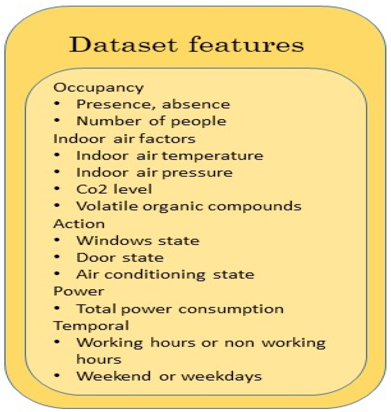
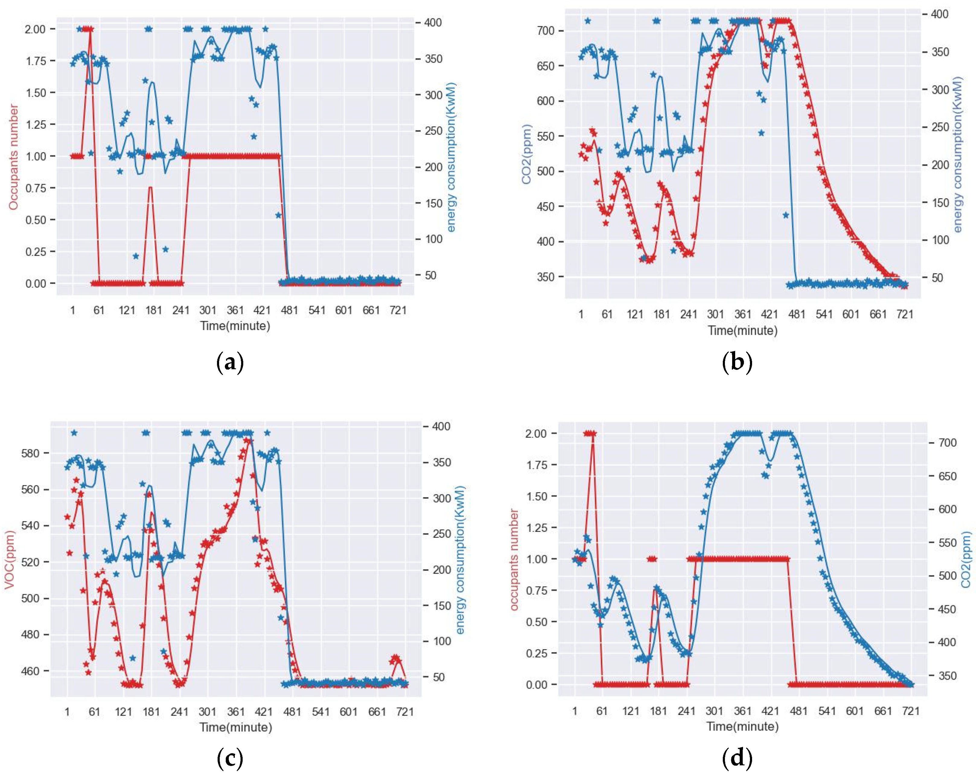
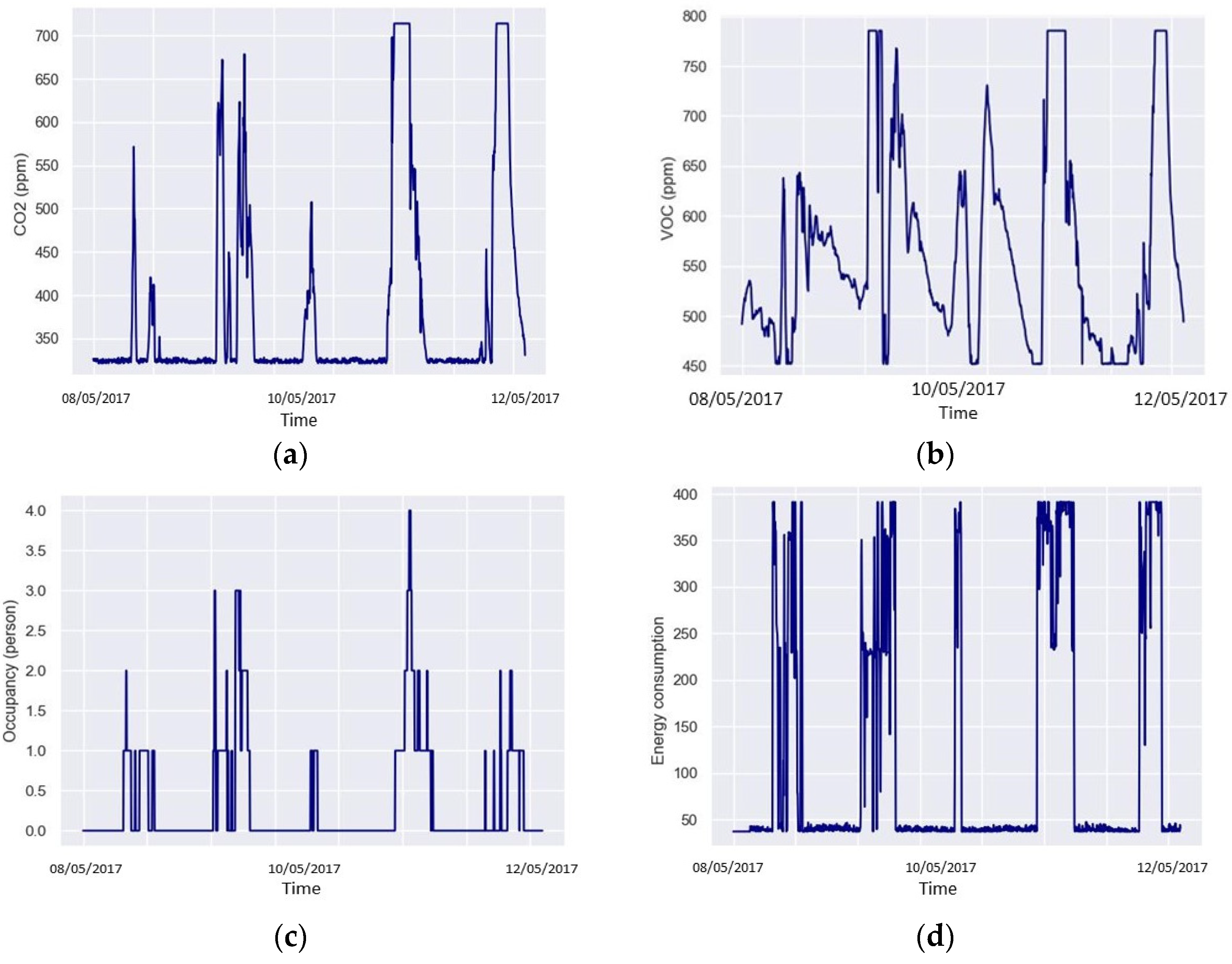
3.1. Dataset Presentation

The dataset in this study was previously collected and is publicly available. The dataset was collected in an office of the University of Calabria, which is a public building located in the south of Italy (39°21′58.6″ N 16°13′30.9″ E) with Mediterranean weather conditions. The area of the concerned office is 19 m² and its height is 2.50 m. The room has two wing windows that face the west. The windows dimensions are 68 × 76 cm. The room is equipped with desktop computers and printers, and its heating and cooling systems are autonomous [25,26]. The data are numerical data. Occupancy data were collected only taking into account the working days and the hours between 8 a.m. and 9 p.m. The occupancy count is performed manually by the person in the monitored office. The considered dataset is sampled every 1 min, from 13 May 2016 to 12 May 2017, using different types of sensors: two CO₂ sensors and air quality thermometers. The state of the door and the window were monitored using magnetic switches. Figure 7 presents the list of measured features of the dataset.

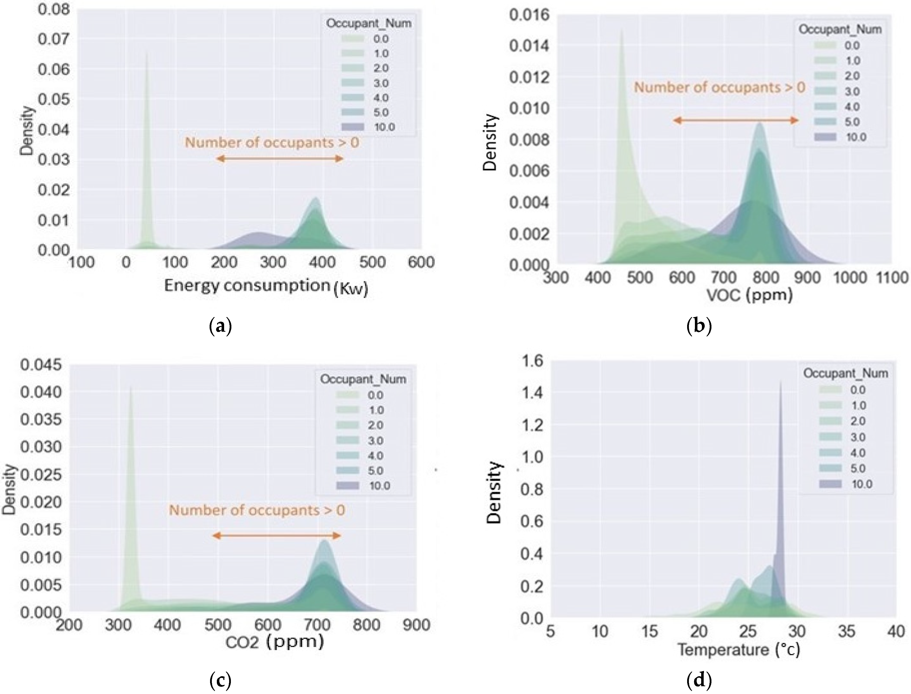
3.2. Dataset Analysis and Processing

The missing values of the dataset are imputed by interpolation techniques. The autocorrelation between each two features is computed based on the following equation:

$$\mathrm{Autocorr}=\frac{\mathrm{Cov}\left({\mathrm{x}}_1\left(\mathrm{t}\right),{ \mathrm{x}}_2\left(\mathrm{t}\right)\right)}{{\mathsf{\sigma }\mathrm{x}}_1\left(\mathrm{t}\right){\mathsf{\sigma }\mathrm{x}}_2\left(\mathrm{t}\right)}$$

(6)

where, ${\mathrm{x}}_1\left(\mathrm{t}\right),{\mathrm{x}}_2(\mathrm{t}$) are the variables at time, Cov is the covariance, and σ is the standard deviation. The three features highly correlated with energy consumption are the number of occupants, CO₂, and volatile organic compounds (VOC). Their correlations are 0.76, 0.64, and 0.45, respectively. CO₂ and VOC are two variables that are directly related to occupants of spaces in closed environments. The autocorrelations between occupants, CO₂, and VOC are 0.63 and 0.45 respectively.

The density of each continuous variable for each number of occupants is presented in Figure 8. In fact, by density, it shows how many times a measurement is repeated for each feature based on different occupancy numbers, and illustrates the distribution.

Figure 8 shows that the densities of energy consumption, VOC, and CO₂ are higher in the presence of occupants, which confirms our prior knowledge regarding autocorrelation. However, as revealed in the case of temperature density and occupancy, there is no clear pattern. It is also seen that the inhalations and exhalations of people affect the CO₂ and VOC measurements. The abovesaid analysis shows that VOC, CO₂, and occupancy data are valid features that can affect the performance of machine learning models.

Considering Figure 8, it is understood that CO₂, VOC, and occupancy play undeniable roles as exogenous data for modeling. In fact, according to Equation (1), while considering them as sole inputs to the model, it could be argued that energy consumption in time t is a function of CO₂, VOC, and occupancy. Relatively, CO₂ and VOC can be considered as a function of occupancy in covered environments:

$$\mathrm{E}\left(\mathrm{t}\right)=\mathrm{f}\left({\mathrm{CO}}_2\left(\mathrm{Occ}\left(\mathrm{t}\right)\right),\mathrm{VOC}\left(\mathrm{occ}\left(\mathrm{t}\right)\right),\mathrm{OCC}\left(\mathrm{t}\right)\right)$$

(7)

where, occ(t) illustrates the occupation level in time t, f is the function that shows the relation of occupancy level to CO₂, g represents the relation between CO₂ and energy consumption, and E(t) depicts the energy consumption in time t. The following equation reveals the effect of changes in occupancy level and CO₂ concentration on energy consumption by a derivative of energy consumption in Equation (8), with respect to occupancy (occ(t)):

$$\frac{\mathrm{dE}\left(\mathrm{t}\right)}{\mathrm{dOCC}}=\left(\frac{\mathrm{df}}{{\mathrm{dCO}}_2}\times \frac{{\mathrm{dCO}}_2}{\mathrm{dOCC}}\right)+\left(\frac{\mathrm{df}}{\mathrm{dVOC}}\ast \frac{\mathrm{dVOC}}{\mathrm{dOCC}}\right)+\frac{\mathrm{df}}{\mathrm{dOCC}}$$

(8)

It shows that the changes in occupancy lead to changes in CO₂, and energy consumption changes following the change in CO₂. Figure 9 shows the variations between the abovementioned features during 12 h, with a granularity of 5 min.

Finally, Figure 10 shows the time series of CO₂, VOC, occupancy, and energy consumption during one working week (five days), which are the selected features for the learning phase. The data granularity is 5 min, and the energy consumption is calculated every five minutes (sum of consumption in watts for every five minutes).

By knowing features that participate in the modeling phase, to prepare the data for the training phase, standardization is performed to scale the input variables. This process adjusts the magnitude of the measured variables and converts them to a common size, as shown in the following equation:

$${\mathrm{X}}_{\mathrm{standardisation}}=\frac{\mathrm{X}-\overline{\mathrm{X}}}{\mathsf{\sigma } }$$

(9)

where, X is the data samples, $\overline{\mathrm{X}}$ is the mean value of the data samples, and $\mathsf{\sigma }$ is the standard deviation of the data. In the next section, experimentation and results of the mentioned dataset are presented.

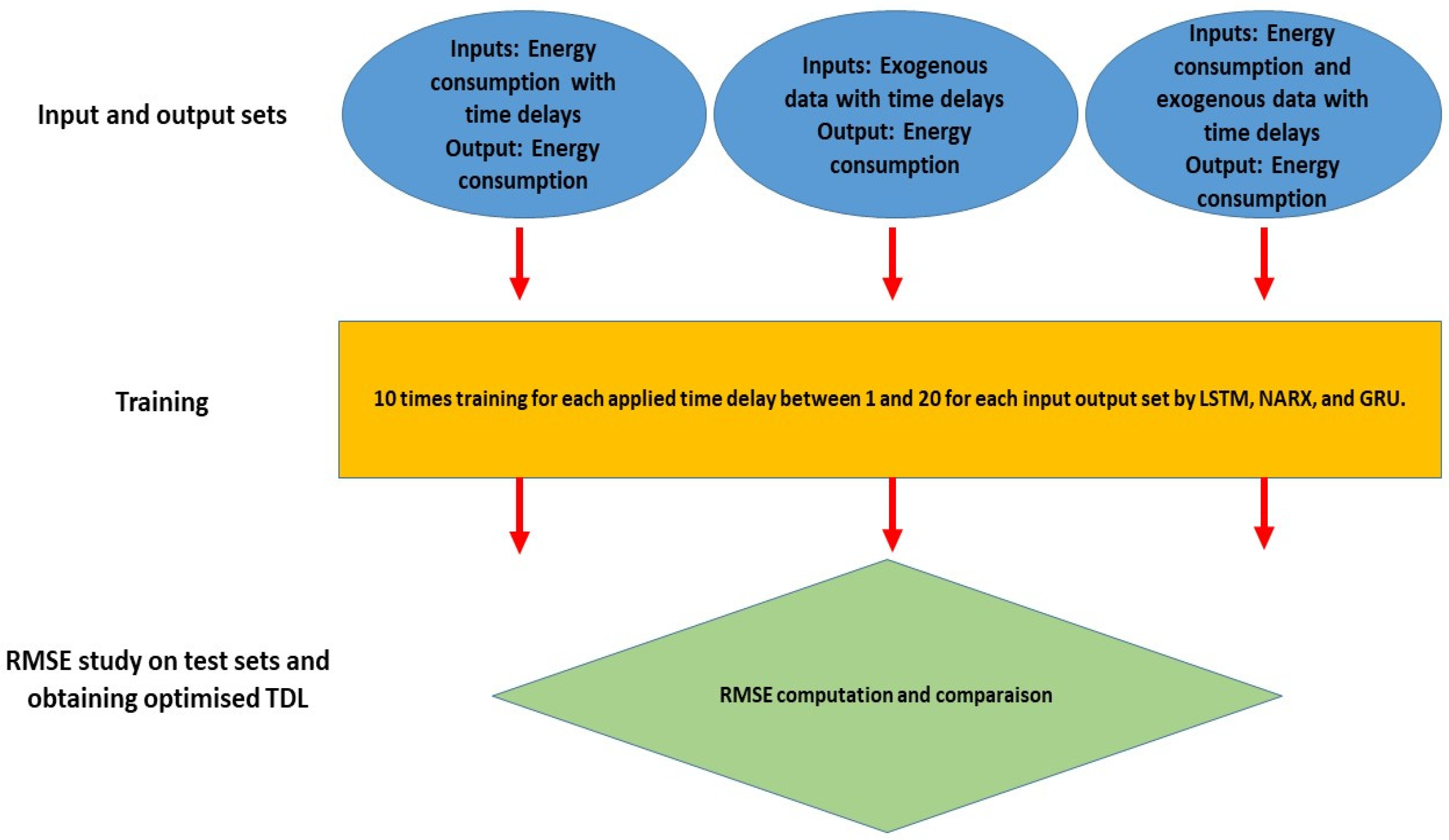
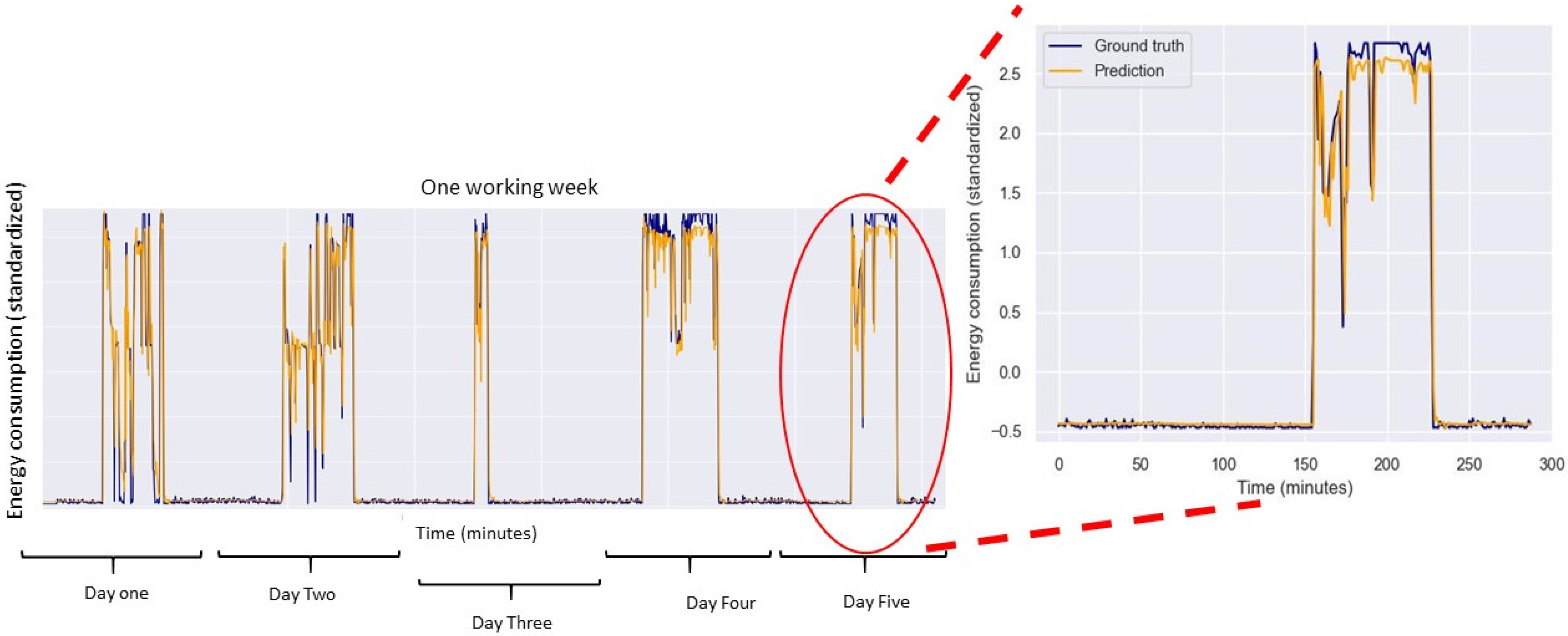
4. Experimentation and Results

The experimentation of this investigation is implemented based on several protocols and criteria. Three different models, based on three types of matched input features, are constructed for each proposed algorithm:

• The first set of input features is the energy consumption with applied time lags (ECTL) to predict the energy consumption in their next steps.
• In the second model, only the exogenous data with applied time lags (ETL), which lacks the energy consumption data, are utilized as inputs to study the model performance and the association of exogenous data.
• In the third model, energy consumption and exogenous data with applied time lags (ECETL) are used as the inputs to study their roles in the final model’s performance.

After finding the appropriate model for each abovementioned case, the model reliance can be implemented to analyze the important features associated with the constructed models. However, before that, it is imperative to find a model with good performance. Applying time lags to features is the most crucial parameter that plays an undeniable role in time series forecasting problems. They affect the computation cost, complexity, and accuracy of the models. Due to this fact, a protocol is presented in the next section to obtain the optimized number of time lags for each case of modeling, based on the different abovementioned input sets.

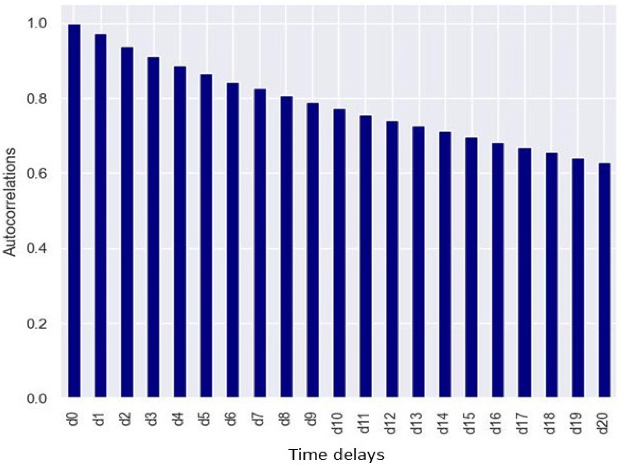
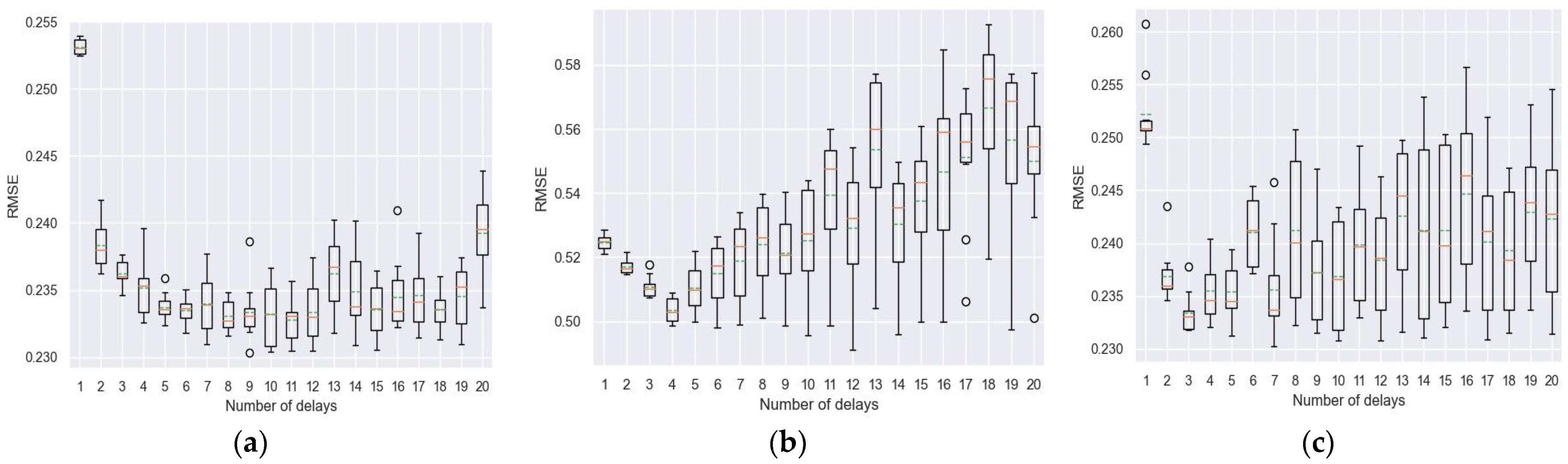
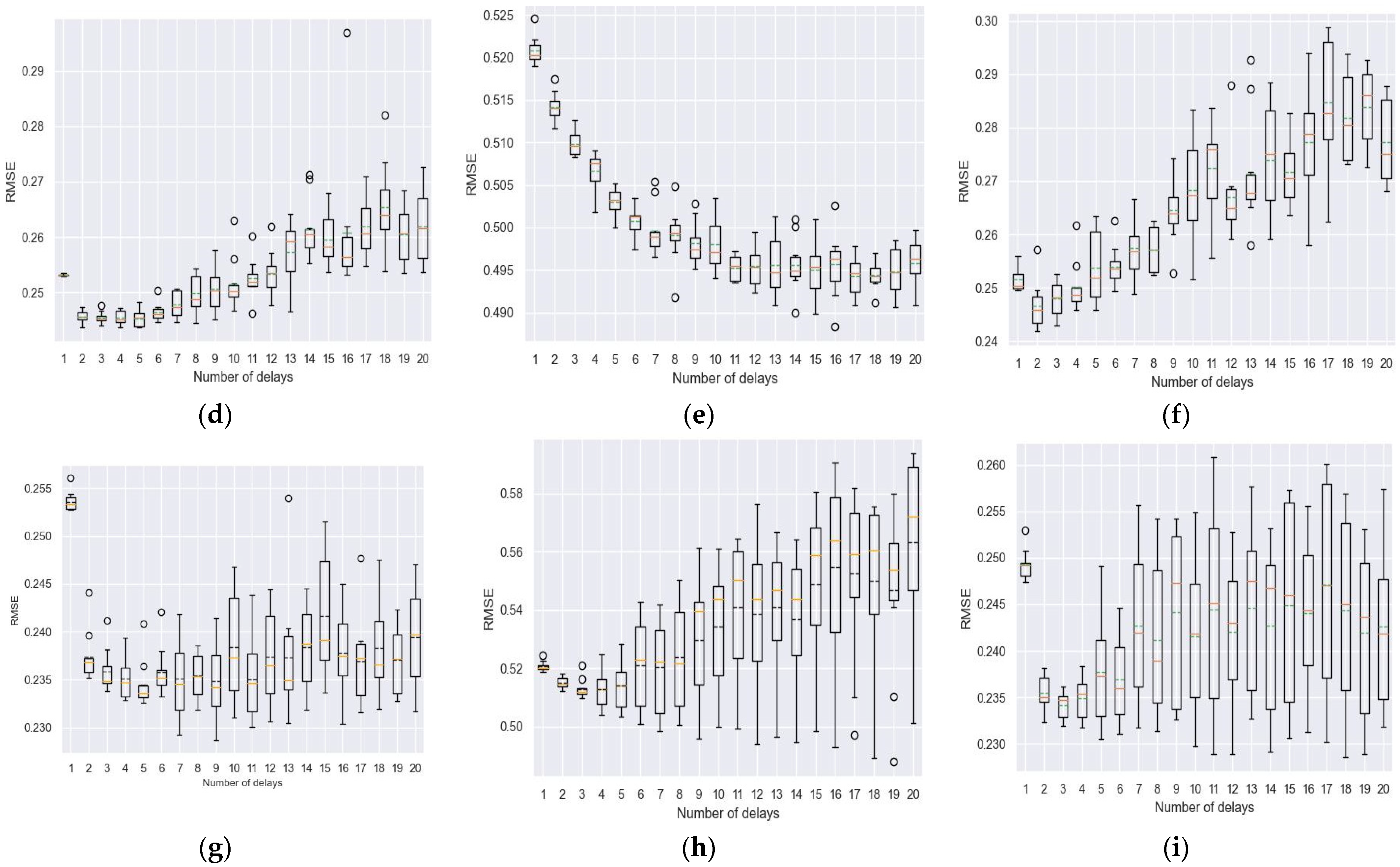
4.1. Experimentation to Realize Tapped Delay Line (TDL)

A critical step in solving time series forecasting problems is choosing past observations (tapped delay lines, time delays, or time lags) to train the models. Time delays provide the neural networks with valuable information. Nevertheless, it can be challenging to adjust historical time step parameters, as the target value’s relationship with the input variables changes over time, and doing so would require high computational costs. Hence, a proper time delay selection method is necessary, as it provides a minimal set of time-correlated historical data, as well as a less complex predictive model.

Considering the abovementioned, an approach is proposed to examine the optimized tapped delay line: observing and studying the root mean square errors of models based on a solid protocol-based approach.

The autocorrelation function is used to determine the relationship between time $\mathrm{t}$ and $\mathrm{t} + \mathrm{k}$. Figure 11 shows the autocorrelations; as illustrated, by increasing the time steps, the autocorrelation declines. The preference is to select the shortest time steps to not only decrease the complexity of the model, but also to keep the time steps that have the most relevant autocorrelation to the target output (energy consumption).

To study the plausibility of the TDL selection method, several models are constructed by LSTM, NARX based on MLP, GRU, decision tree, and XGboost. For each delay between 1 and 20, the training and testing are performed 10 times to evaluate the models; in each training phase, the weights and biases are initialized randomly (200 models for LSTM, NARX, and GRU for each predefined feature set as inputs). Regarding the decision tree and XGboost, 20 models are constructed for each set of inputs. Considering three sets of inputs, the total number of trained models is 1920. The process of implementation is performed by Python and by several machine learning and deep learning packages. The hyperparameters for NARX, LSTM, and GRU are configured by Bayesian grid search techniques and by trial and error. Of the data, 80 percent is used for training and 20 percent is used for testing. Regarding NARX-MLP, after several trials and errors, two hidden layers with sizes of 25 and 6, with a tangent hyperbolic activation function, are utilized. The maximum iteration is 30. Referring to LSTM and GRU, two layers with sizes of 32 and 16 are used. The activation functions for the two are rectified linear unit (ReLU) and scaled exponential linear unit (SeLU). The batch size is 128 with 10 epochs. Finally, the maximum, minimum, and average root mean square errors of the models for each TDL are computed. Regarding decision tree and XGboost hyperparameters, a grid search is implemented. Figure 12 presents the graph of the implementation of the protocol. The same protocol is implemented for decision tree and XGboost. However, instead of training 10 times for each time delay, a search grid is implemented (as decision tree training is not based on the initialization of weights).

According to Figure 13, for each curve, the optimum time delay is estimated for each model and the related algorithm. As shown in the figure, the consequence of increasing the time lags is the growth of errors and a bigger distribution of errors. Indeed, the enlargement of time lags does not improve the model’s performance, and it makes the problem more complex. In the first case (Figure 13a,d), where solely the energy consumption delays are used as the inputs to the models, delay number 10 (in the acceptable range of 10 to 12) and delay number 3 (in the acceptable range of 2 to 5) are selected for LSTM and NARX, respectively. For the first case, due to reducing the computational cost and a lower median and minimum error, a delay of 10 is selected. In the second case, in delay three, the average and median of the RMSE are smaller than two, and comparing delay three to delay four, the computational cost is less. The defined ranges are the optimum of the curves. The same approach is followed for the rest to obtain the optimized value of time delays.

Finally, the models are assessed by the calculation of three metrics, RMSE (root mean squared error), MAE (mean absolute error), and ${\mathrm{R}}^2$ (R-squared), defined, respectively, as follows:

$$\mathrm{RMSE}=\sqrt{\frac{1}{\mathrm{N}}{\sum }_{\mathrm{i}=\mathrm{n}}^{\mathrm{n}}{\left({\mathrm{y}}_{\mathrm{i}}-\widehat{{\mathrm{y}}_{\mathrm{i}}}\right)}^2}$$

(10)

$$\mathrm{MAE}=\frac{{\sum }_{\mathrm{i}=1}^{\mathrm{n}}\left|{\mathrm{y}}_{\mathrm{i}}-\widehat{{\mathrm{y}}_{\mathrm{i}}}\right|}{\mathrm{N}}$$

(11)

$${ \mathrm{R}}^2=1-\frac{{\sum }_{\mathrm{i}=1}^{\mathrm{n}}{\left({\mathrm{y}}_{\mathrm{i}}-\widehat{{\mathrm{y}}_{\mathrm{i}}}\right)}^2}{{\sum }_{\mathrm{i}=1}^{\mathrm{n}}{({\mathrm{y}}_{\mathrm{i}}-\overline{\mathrm{y}})}^2}$$

(12)

where, ${\mathrm{y}}_{\mathrm{i}}$ is the actual energy consumption, $\hat{\mathrm{y}}$ is the predicted energy consumption, and n is the number of samples.

Table 1. Results summary of model performances based on different input features based on LSTM, NARX, GRU, decision tree, and XGboost.

Models	Algorithm	Time Lags	RMSE-MIN	RMSE-MAX	MAE-MIN	MAE-MAX	R2-MIN	R2-MAX
1. ECTL	LSTM	10	0.23	0.234	0.072	0.085	0.95	0.95
	NARX	4	0.243	0.247	0.077	0.082	0.944	0.946
	GRU	3	0.23	0.24	0.069	0.078	0.94	0.95
	Decision tree	7	0.234		0.072		0.95
	XGboost	8	0.232		0.073		0.95
2. ETL	LSTM	4	0.49	0.50	0.22	0.24	0.76	0.77
	NARX	15	0.48	0.50	0.21	0.23	0.77	0.78
	GRU	5	0.50	0.52	0.20	0.24	0.74	0.77
	Decision tree	12	0.50		0.22		0.77
	XGboost	18	0.48		0.22		0.78
3. ECETL	LSTM	3	0.23	0.237	0.07	0.08	0.94	0.95
	NARX	3	0.24	0.25	0.08	0.089	0.942	0.946
	GRU	3	0.23	0.236	0.07	0.09	0.94	0.95
	Decision tree	2	0.234		0.072		0.95
	XGboost	10	0.22		0.073		0.95

presents the results regarding the models with the optimized number of time delays for each case.

In addition to assessing the models individually, for comparing the accuracy of the models, each against the other, the Diebold–Mariano (DM) test is implemented [27,28,29]. It is a statistical approach that permits us to make a comparison of the prediction accuracy. It assumes:

$$\mathrm{Assumption} \mathrm{DM}:\left\{\begin{array}{c}\mathrm{E}\left({\mathrm{d}}_{12\mathrm{t}}\right)=\mathsf{\mu },\forall \mathrm{t}\\ \mathrm{Cov}\left({\mathrm{d}}_{12\mathrm{t}},{\mathrm{d}}_{12\left(\mathrm{t}-\mathsf{\tau }\right)}\right)=\gamma \left(\mathsf{\tau }\right),\\ 0<\mathrm{var}\left({\mathrm{d}}_{12\mathrm{t}}\right)={\mathsf{\sigma }}^2<\infty \end{array}\right.\forall \mathrm{t}$$

(13)

where, d₁₂ is the loss differential between predictions one and two. E(d₁₂) represents the hypothesis of equal predictive accuracy, which is E(d₁₂) = 0, under the retained assumption DM:

$${\mathrm{DM}}_{12}=\frac{{\overline{\mathrm{d}}}_{12}}{{\widehat{\mathsf{\sigma }}}_{{\overline{\mathrm{d}}}_{12}}}\stackrel{\mathrm{d}}{\to } \mathrm{N}\left(0,1\right)$$

(14)

where, ${\overline{\mathrm{d}}}_{12}$ is the average of the sample of loss differential and ${\widehat{\mathsf{\sigma }}}_{{\overline{\mathrm{d}}}_{12}}$ is a consistent estimate of the standard deviation of ${\overline{\mathrm{d}}}_{12}$. If the assumption of DM is maintained, consequently, the $\mathrm{N}\left(0,1\right)$, which is the limiting distribution of the static test, should be preserved.

To begin, it has to be noted that in the case of decision tree and XGboost there is just one value for each metric, which is due to the different configurations of decision tree and XGboost. NARX, GRU, and LSTM are neural networks and, in the training phase, each of the time weight biases are initialized randomly. However, decision tree and XGboost fit the data based only on tuning of the hyperparameters. The best performance, by considering RMSE as the critical condition, is achieved by the LSTM and GRU models, with the energy consumption time delay (ECTL) selected as input. The RMSE for the concerned models is 0.23. However, GRU achieved this RMSE by 3 time lags, and LSTM by 10 time lags. The time delay in the case of ECTL for LSTM is higher than all of the other algorithms. However, it should be noted that, for instance, according to Figure 13a,d, LSTM still has a better performance than NARX in time lag four. In addition, the selected time lag of 10 does not mean that LSTM could not perform better with a less computationally demanding and complex model.

In the case where only ambient data is used for modeling (ETL model), concerning RMSE values and the number of delays, GRU and LSTM perform the opposite of other algorithms. LSTM and GRU have lower error in lower time lags, but on the other hand, other algorithms need more historical data in order to perform as well as LSTM and GRU. This indicates their ability to achieve better results with lower historical data, in this case. Although, NARX and decision tree, in two other cases (ECTL and ECETL) and with lower time lags (two and three), performed more comparably. In the case of ECETL, it should be mentioned that decision tree with a lower number of time lags has a better performance than NARX, and a little higher than GRU and LSTM.

In general, while energy consumption is included in the input data, the performance of the models is much higher than in the case where only the ambient data is utilized as input. In both MAE and RMSE criteria, the performances of the models for ECTL and ECETL are comparable, with a slightly better performance for ECTL. However, it should be noted that in conditions where multistep prediction (where the predicted energy consumption is output with a closed-loop feedback to the input) is considered, the exogenous data will influence the performance, and ECETL can show its advantage over the other two [21]. Figure 14 presents the prediction of energy consumption during one working week, and the zoomed in portion shows one working day (for better visualization) by LSTM-ECTL.

In order to compare the prediction accuracy of each model to the other models, according to selected optimized time delays, the Diebold–Mariano test is applied. To this end, for each model (named ECTL, ETL, ECETL), based on optimized time lag setting for each algorithm based on Table 1, the following table is presented to compare the performance of modeling with different algorithms. Despite the abovementioned metrics based on the RMSE, MAE, and R², the DM test yields a statistical view of the prediction accuracy of each constructed model compared to the others.

According to

Table 2. Results summary of model accuracy comparisons by the Diebold–Mariano test for each model case and implemented machine learning algorithms.

Models	Algorithms	XGboost		LSTM		NARX		GRU
		DM	p-Value	DM	p-Value	DM	p-Value	DM	p-Value
1. ECTL	LSTM	−1.86	0.031	---	---	---	---	---	---
	NARX	5.35	0.99	6.56	1	---	---	---	---
	GRU	0.86	0.8	2.51	0.99	−5.28	6.42$\times {10}^{-8}$	---	---
	Decision tree	1.047	0.85	2.42	0.99	−4.83	6.85$\times {10}^{-7}$	0.277	0.609
2. ETL	LSTM	4.53	0.99	---	---	---	---	---	---
	NARX	0.70	0.75	−3.88	5.22$\times {10}^{-5}$	---	---	---	---
	GRU	8	1	2.8	0.99	6.45	1	---	---
	Decision tree	5.4	0.99	0.52	0.701	4.56	0.99	−1.3	0.096
3. ECETL	LSTM	2.03	0.97	---	---	---	---	---	---
	NARX	7.78	1	6.17	1	---	---	---	---
	GRU	2.87	0.99	0.135	0.55	−5.55	1.43$\times {10}^{-8}$	---	---
	Decision tree	3.05	0.99	1.39	0.91	−3.49	0.0002	1.288	0.90

and ECTL, comparing LSTM with the four other algorithms, the p-value is greater than the threshold of 0.05. This indicates that there is no evidence that LSTM and the other models have a statistical advantage over each other, in the case of prediction accuracy. However, the DM value reveals the slightly better performance of the other models over LSTM. Comparing NARX with GRU and decision tree, the p-value is very low (lower than the threshold), which indicates the accuracy of prediction is different. The negative value of DM shows the better performance of NARX over the two mentioned algorithms. The result of the DM test for the comparison of GRU with decision tree and XGboost also shows no clear evidence of better-performing models, due to the high p-value. The results of ECETL, in almost all cases, also follow the results of ECTL, except in the case of LSTM and XGboost in ECETL, in which, in contrast to ECTL, LSTM has slightly better performance over XGboost. Considering Table 1, these two models also have very close metrics values that confirm the results of Table 2.

With regards to ETL, for the case of comparing NARX and LSTM, the p-value of 5.22$\times {10}^{-5}$, which is smaller than the threshold of 0.005, shows that there are statistical differences in the model’s prediction accuracy. In addition, the value of −3.88 confirms that the modeling by LSTM, in this case, is better than NARX. The comparison of XGboost with decision tree, LSTM, and NARX reveals the same results, that there are no statistical differences between the models due to their high p-values. Although, regarding decision tree and GRU, the p-value is 0.096, and there is a slightly better performance of GRU over decision tree. To sum up, considering ECTL and ECETL, all models do not have meaningful differences, except in the case of comparing NARX to decision tree and GRU. In this case, the p-value is smaller than the threshold, and shows a clear advantage of NARX. It is the same for ETL, where the p-values for NARX and LSTM show a better performance of LSTM. Despite slight differences between RMSE, MAE, and DM, the time lags of each model should not be forgotten when making model selection decisions. As an example, while for ECETL the performance of the model, in the case of LSTM and GRU, is almost the same, the time lags for GRU is 3, while for LSTM it is 10, which makes the model more complex and has a higher computational cost. In the next section of this paper, the experimental results of model reliance on input features are analyzed.

4.2. Experimental Results Regarding Model Reliance

At this stage of the investigation, a deeper analysis of participant input data is performed by the model reliance method. The proposed method is implemented in two different scenarios:

1.

Exploring the model reliance score on input features.

2.

Exploring the model reliance score on time delay layers.

This will assist in the discovery of imperative data that are associated with model construction.

Table 3. Results summary of model reliance on input features (in the case of LSTM, NARX, GRU, decision tree, and XGboost models).

			Model Reliance Score
Models	Algorithm	Time Lags	Energy Consumption	VOC	CO2	Occupancy
1. ECTL	LSTM	10	4.95	---	---	---
	NARX	4	6.50	---	---	---
	GRU	3	4.92	---	---	---
	Decision tree	7	6.88	---	---	---
	XGboost	8	6.92	---	---	---
2. ETL	LSTM	4	---	1.11	1.35	1.98
	NARX	15	---	1.064	1.14	2.81
	GRU	5	---	1.083	1.24	1.99
	Decision tree	12	---	1.11	1.23	2.83
	XGboost	18	---	1.25	1.57	2.73
3. ECETL	LSTM	3	4.68	1.018	1.005	1.10
	NARX	3	6.15	1.007	1.03	1.22
	GRU	3	4.71	1.011	1.003	1.11
	Decision tree	2	6.58	1.001	1.004	1.41
	XGboost	10	6.78	1.003	1.012	1.17

presents the results of the models’ reliance on input features. Regarding ECTL, as there is only one input feature, clearly the model reliance score is high, equal to 4.95, 6.5, 4.92, 6.88, and 6.92 for LSTM, NARX, GRU, decision tree, and XGboost, respectively. Considering all of the models, and apart from energy consumption as input, occupancy is associated with modeling more than CO₂ and VOC data. It is noteworthy that occupancy data is more correlated (based on the autocorrelation table) to energy consumption than the two others, and as mentioned in Section 3.2, Equation (7), CO₂ and VOC are functions of occupancy, which is confirmed by the reliance model. The MR score of almost 1 indicates it does not affect the model performance too much. Regarding ECTL and ECETL, Table 3 shows that when lacking exogenous data, LSTM and NARX are more under the influence of energy consumption as the only input.

In the next step of the analysis, as promised, MR is applied to time delay slices for the most important features that have the higher scores. Figure 15 presents MR scores versus time delays of the most important features, according to Table 3 (features with the highest MR scores). They are energy consumption for the first and third case, and occupancy for the second case. In all situations, despite a slight fluctuation, a declining orientation is observed from d1 (which is one time step before the predicted output) to further time steps. Indeed, delayed d1 is the most correlated to the output of the model (as is also illustrated in Figure 11). It is interesting to note that all MR scores of time delays are higher than 1, which shows the effectiveness of the approach to choose the optimum time delays in the last section of the investigation. By considering Figure 11 and Figure 13, it is important to stress that delay number one has a high score, based on Figure 13. However, modeling by considering only the delay number one is the worst approach, based on the RMSE results in Figure 13. It denotes that, despite the high score of delay one and the low score of other delays in Figure 14, the other delays play a crucial role in augmenting the performance of the models.

The comparison of the MR scores between the algorithms illustrates that the absolute slope values between d1 and d2 in the case of NARX and XGboost, and decision tree in all cases, is higher than LSTM and GRU. It indicates that NARX, XGboost, GRU rely more on d1 for the construction of the model than LSTM and GRU.

While other techniques such as autocorrelation are useful for selecting appropriate features before modeling, the model reliance method, as a complementary approach after modeling, should be used. It not only confirms or disconfirms the result of other methods, but also indicates, with higher reliability, the role of features in modeling and analysis, and if the model is optimized and performs well in the context of computational cost and accuracy.

Ultimately, based on the obtained results, ECTL and ECETL show their higher performance compared to ETL, due to energy consumption as a key feature in the input data. MR also confirmed that it has a higher score and is associated with the learning phase more than the other features. The metrics and DM results also show that the differences between ECTL and ECETL are not high. However, except XGboost, other algorithms with lower time lags achieved high performance regarding ECETL. This indicates that providing more features to the model leads to a decreased number of delays, while the models perform almost the same. Based on the type of problem to be solved, one of these two models can be considered. While the RMSE, MAE, and R² metrics illustrate comparable results between different algorithms for each case of modeling, DM more clearly shows the advantage of each model to the other one; as an example, for the case of ECTL, NARX performs better than GRU and decision tree. Regarding ECETL and ECTL, due to fewer time lags for NARX compared to LSTM and GRU, and a lower complexity of the algorithm, NARX is a better choice. The result of DM also confirms that NARX forecasts better than decision tree and XGboost. However, considering ETL, LSTM shows its advantages for finding better models with lower time lags, according to DM analysis. It seems that LSTM and GRU can achieve better results for modeling from time sequences, while there are fewer input features correlated to the output, and lower MR scores. It shows the capability of LSTM and GRU when the problem is more complex and nonlinear. In other cases, where correlation is high between the input and output, and there is a high MR score in the features, NARX can capture the dependencies efficiently and construct a model with better performance.

While the RMSE, MAE, and R² are perfect metrics for finding models with the desired performance, the DM test, as an important complementary analysis method, reveals its usefulness for selecting a model when the other metrics show comparable results.

5. Conclusions

In this article, an approach for modeling a well-performing energy consumption forecasting model is proposed and analyzed. This article has three stages for modeling and analyzing. In the first stage, the inputs that are most correlated to the outputs are selected, and, according to defined protocols, three different types of models based on different inputs are constructed by two well-known algorithms in this domain, which are LSTM, NARX by MLP, GRU, decision tree, and XGboost. In the second stage of this article, an efficient approach is utilized to obtain the best time delays for each proposed model. The goal is to optimize the number of time delays parameter to achieve a less complex model that has the highest performance. The highest performance is achieved with ECTL and ECETL, where they perform with almost 0.07 as the minimum MAE. The lowest performance is exhibited by the models where the input features are solely ambient data (ETL). The MAE of these models for LSTM, NARX, GRU, decision tree, and XGboost are 0.22, 0.21, 0.2, 0.22, and 0.22, respectively. The DM test is also clarified, statistically, the accuracy of the models’ predictions. In most cases, it confirms that there is not much difference between the models, as illustrated by the resulting metrics. In the last stage, the model reliance method is applied in order to quantify the contribution of features and time delays in the constructed models. The results show that, in the case of modeling just with ambient data, occupancy participates the most; in the other two cases, it is the energy consumption with time lags. Regarding the time delay MR score, the highest model reliance score is achieved by the first time lag. As the time step increases, the score falls. The results of the model reliance analysis also confirm the proposed method regarding obtaining an optimized number of delays as, in all cases, the scores are higher than 1. In the end, among utilized algorithms for modeling of ECETL and ECTL, NARX, with less complex architecture and computation, appears to be a better choice for this case study. Where the input and output features are not highly correlated, and the model’s MR score is low, which is the ETL case, LSTM appears to be the better choice.

The present approach can apply to any time series problem, especially in the sector of energy and buildings, where the researchers are facing highly dynamic parameters that affect the modeling performance. It can quantify the selection of different models by different metrics and statistical tests according to different settings of time lags to optimize their number. In future work, the proposed approach serves to construct a predictive application to plan energy management systems in buildings or microgrids.

References

1. Herrington, G. Update to limits to growth: Comparing the World3 model with empirical data. J. Ind. Ecol. 2021, 25, 614–626. [Google Scholar] [CrossRef]
2. Ministry of Ecological and Solidarity Transition. Multi Annual Energy Plan; Ministre de la Transition Ecologique et Solidaire: Paris, France, 2019; p. 342. [CrossRef]
3. Énergie dans les Bâtiments|Ministères Écologie Énergie Territoires (n.d.). Available online: https://www.ecologie.gouv.fr/energie-dans-batiments (accessed on 22 September 2022).
4. Koschwitz, D.; Frisch, J.; van Treeck, C. Data-driven heating and cooling load predictions for non-residential buildings based on support vector machine regression and NARX Recurrent Neural Network: A comparative study on district scale. Energy 2018, 165, 134–142. [Google Scholar] [CrossRef]
5. Rahman, A.; Srikumar, V.; Smith, A.D. Predicting electricity consumption for commercial and residential buildings using deep recurrent neural networks. Appl. Energy 2018, 212, 372–385. [Google Scholar] [CrossRef]
6. Xue, P.; Jiang, Y.; Zhou, Z.; Chen, X.; Fang, X.; Liu, J. Multi-step ahead forecasting of heat load in district heating systems using machine learning algorithms. Energy 2019, 188, 116085. [Google Scholar] [CrossRef]
7. De Silva, M.; Sandanayake, Y. Building Energy Consumption Factors: A Literature Review and Future Research Agenda. 2012. Available online: http://dl.lib.uom.lk/handle/123/12050 (accessed on 8 December 2022).
8. Hadjout, D.; Torres, J.F.; Troncoso, A.; Sebaa, A.; Martínez-Álvarez, F. Electricity consumption forecasting based on ensemble deep learning with application to the Algerian market. Energy 2022, 243, 123060. [Google Scholar] [CrossRef]
9. Chi, D. Research on electricity consumption forecasting model based on wavelet transform and multi-layer LSTM model. Energy Rep. 2022, 8, 220–228. [Google Scholar] [CrossRef]
10. Dong, B.; Liu, Y.; Mu, W.; Jiang, Z.; Pandey, P.; Hong, T.; Olesen, B.; Lawrence, T.; O’Neil, Z.; Andrews, C.; et al. A Global Building Occupant Behavior Database. Sci. Data 2022, 9, 369. [Google Scholar] [CrossRef]
11. Chen, S.; Ren, Y.; Friedrich, D.; Yu, Z.; Yu, J. Prediction of office building electricity demand using artificial neural network by splitting the time horizon for different occupancy rates. Energy AI 2021, 5, 100093. [Google Scholar] [CrossRef]
12. Amasyali, K.; El-Gohary, N. Building Lighting Energy Consumption Prediction for Supporting Energy Data Analytics. Procedia Eng. 2016, 145, 511–517. [Google Scholar] [CrossRef]
13. Faiq, M.; Geok Tan, K.; Pao Liew, C.; Hossain, F.; Tso, C.P.; Li Lim, L.; Khang Wong, A.Y.; Mohd Shah, Z. Prediction of energy consumption in campus buildings using long short-term memory. Alex. Eng. J. 2023, 67, 65–76. [Google Scholar] [CrossRef]
14. Mahjoub, S.; Chrifi-Alaoui, L.; Marhic, B.; Delahoche, L. Predicting Energy Consumption Using LSTM, Multi-Layer GRU and Drop-GRU Neural Networks. Sensors 2022, 22, 4602. [Google Scholar] [CrossRef]
15. Lin, X.; Yu, H.; Wang, M.; Li, C.; Wang, Z.; Tang, Y. Electricity consumption forecast of high-rise office buildings based on the long short-term memory method. Energies 2021, 14, 4785. [Google Scholar] [CrossRef]
16. Gers, F.A.; Schmidhuber, J.; Cummins, F. Learning to forget: Continual prediction with LSTM. Neural Comput. 2000, 12, 2451–2471. [Google Scholar] [CrossRef]
17. Tang, X.; Dai, Y.; Wang, T.; Chen, Y. Short-term power load forecasting based on multi-layer bidirectional recurrent neural network. Undefined 2019, 13, 3847–3854. [Google Scholar] [CrossRef]
18. Vanishing and Exploding Gradients in Deep Neural Networks (n.d.). Available online: https://www.analyticsvidhya.com/blog/2021/06/the-challenge-of-vanishing-exploding-gradients-in-deep-neural-networks/ (accessed on 19 September 2022).
19. Wang, J.Q.; Du, Y.; Wang, J. LSTM based long-term energy consumption prediction with periodicity. Energy 2020, 197, 117197. [Google Scholar] [CrossRef]
20. LSTM RNN in Keras: Examples of One-to-Many, Many-to-One & Many-to-Many–Weights & Biases (n.d.). Available online: https://wandb.ai/ayush-thakur/dl-question-bank/reports/LSTM-RNN-in-Keras-Examples-of-One-to-Many-Many-to-One-Many-to-Many---VmlldzoyMDIzOTM (accessed on 8 December 2022).
21. Broujeny, R.S.; Madani, K.; Chebira, A.; Amarger, V.; Hurtard, L. Data-driven living spaces’ heating dynamics modeling in smart buildings using machine learning-based identification. Sensors 2020, 20, 1071. [Google Scholar] [CrossRef] [Green Version]
22. Ng, B.C.; Darus, I.Z.M.; Jamaluddin, H.; Kamar, H.M. Dynamic modeling of an automotive variable speed air conditioning system using nonlinear autoregressive exogenous neural networks. Appl. Therm. Eng. 2014, 73, 1255–1269. [Google Scholar] [CrossRef]
23. Fisher, A.; Rudin, C.; Dominici, F. All Models are Wrong, but Many are Useful: Learning a Variable’s Importance by Studying an Entire Class of Prediction Models Simultaneously. arXiv 2018, arXiv:1801.01489. [Google Scholar]
24. Chen, T.; Guestrin, C. XGBoost: A scalable tree boosting system. In Proceedings of the 22nd ACM SIGKDD International Conference on Knowledge Discovery and Data Mining, San Francisco, CA, USA, 13 August 2016; pp. 785–794. [Google Scholar]
25. ASHRAE Global Occupant Behavior Database|Kaggle (n.d.). Available online: https://www.kaggle.com/datasets/claytonmiller/ashrae-global-occupant-behavior-database (accessed on 21 September 2022).
26. Mora, D.; Fajilla, G.; Austin, M.C.; de Simone, M. Occupancy patterns obtained by heuristic approaches: Cluster analysis and logical flowcharts. A case study in a university office. Energy Build. 2019, 186, 147–168. [Google Scholar] [CrossRef]
27. Shah, I.; Iftikhar, H.; Ali, S.; Wang, D. Short-term electricity demand forecasting using components estimation technique. Energies 2019, 12, 2532. [Google Scholar] [CrossRef] [Green Version]
28. Diebold, F.X.; Mariano, R.S. Comparing Predictive Accuracy. J. Bus. Econ. Stat. 2002, 20, 134–144. [Google Scholar] [CrossRef]
29. Diebold, F.X. Comparing Predictive Accuracy, Twenty Years Later: A Personal Perspective on the Use and Abuse of Diebold–Mariano Tests. J. Bus. Econ. Stat. 2015, 33, 1. [Google Scholar] [CrossRef] [Green Version]
Figure 1. Proposed protocol: schema of the advancement in the proposed research.
Energies 16 04065 g001
Figure 2. The architecture of LSTM cell with gates formulations.
Energies 16 04065 g002
Figure 3. The architecture of NARX-MLP with output formulation.
Energies 16 04065 g003
Figure 4. The architecture of GRU with gates formulation.
Energies 16 04065 g004
Figure 5. A schema of decision tree architecture.
Energies 16 04065 g005
Figure 6. A schema of XGboost architecture.
Energies 16 04065 g006
Figure 7. Feature details of the dataset.
Energies 16 04065 g007
Figure 8. The density of some continuous features versus their ground truth values: (a) energy consumption for occupancy classes for the dataset, (b) VOC for occupancy classes for the dataset, (c) CO2 for occupancy classes for the dataset, and (d) temperature for occupancy classes for the dataset.
Energies 16 04065 g008
Figure 9. Data visualization of selected features, considering their variation against energy consumption during 12 h of a randomly selected working day: (a) occupant number and energy consumption, (b) CO2 variations and energy consumption, (c) VOC variations and energy consumption, (d) fluctuation of occupant number and CO2. The red and blue points are data points and blue and red lines are the fitted lines to data points.
Energies 16 04065 g009
Figure 10. The time series curves of selected features during one working week, between 8 May 2017 and 12 May 2017: (a) CO2 time series, (b) VOC time series, (c) occupancy numbers time series, (d) energy consumption time series.
Energies 16 04065 g010
Figure 11. Autocorrelation between the time lags of energy consumption (d0 is responsible for no time lags, and d1 to d20 are the first to twentieth time lags of energy consumption, respectively).
Energies 16 04065 g011
Figure 12. Implemented protocol to obtain optimized time delay for each model based on input sets.
Energies 16 04065 g012
Figure 13. Boxplot of the RMSE for ten models for each time delay: (a) ECTL by LSTM, (b) ETL by LSTM, (c) ECETL by LSTM, (d) ECTL by NARX, (e) ETL by NARX, (f) ECETL by NARX, (g) ECTL by GRU, (h) ETL by GRU, (i) ECETL by GRU (average: green dotted line; median: yellow line).
Energies 16 04065 g013aEnergies 16 04065 g013b
Figure 14. The prediction of energy consumption by LSTM-ECTL during one working week, and one working day (12 May 2017–13 May 2017).
Energies 16 04065 g014
Figure 15. Model reliance score relating to time delays for each case of experimentation: (a) LSTM, (b) NARX, (c) GRU, (d) Decision tree, and (e) XGboost.
Energies 16 04065 g015