A Hybrid Model of VMD-EMD-FFT, Similar Days Selection Method, Stepwise Regression, and Artificial Neural Network for Daily Electricity Peak Load Forecasting

Abstract

Daily electricity peak load forecasting is important for electricity generation capacity planning. Accurate forecasting leads to saving on excessive electricity generating capacity, while maintaining the stability of the power system. The main challenging tasks in this research field include improving forecasting accuracy and reducing computational time. This paper proposes a hybrid model involving variational mode decomposition (VMD), empirical mode decomposition (EMD), fast Fourier transform (FFT), stepwise regression, similar days selection (SD) method, and artificial neural network (ANN) for daily electricity peak load forecasting. Stepwise regression and similar days selection method are used for input variable selection. VMD and FFT are applied for data decomposition and seasonality capturing, while EMD is employed for determining an appropriate decomposition level for VMD. The hybrid model is constructed to effectively forecast special holidays, which have different patterns from other normal weekdays and weekends. The performance of the hybrid model is tested with real electricity peak load data provided by the Electricity Generating Authority of Thailand, the leading power utility state enterprise under the Ministry of Energy. Experimental results show that the hybrid model gives the best performance while saving computation time by solving the problems in input variable selection, data decomposition, and imbalance data of normal and special days in the training process.

1. Introduction

Electricity is the main source of energy driving industries and modern life. Electricity load corresponds to economic and population growth. To maintain electricity power stability, electricity generating capacity planning is an essential task that requires accurate electricity load forecasting. Finding the balance between production and consumption by using the potential of the forecasting model is the goal of electricity load forecasting [1]. Accurate electricity load forecasting can reduce the risk of power outages and the cost of excessive electricity generating capacity, especially for short-term load forecasting, which involves more uncertainty than long-term aggregated planning. Basically, short-term load forecasting uses an hourly to weekly load forecasting range and is applied for controlling power security, scheduling power plant operations, and planning load dispatching [2,3,4,5,6].

In general, electricity forecasting methodology can be separated into two main types of techniques, which are statistical techniques and machine learning techniques. The most popular statistical technique used in electricity forecasting problems is the statistical linear regression model [7,8] followed by the Holt Winter’s exponential smoothing model [9], autoregressive moving average model [10], grey model [11], and semi-functional partial linear model [12]. However, statistical techniques have a limitation of nonlinear assumption due to a lack of efficiency to reflect the nonlinear patterns that appear in the recent load trend [13]. To overcome this limitation, machine learning techniques, such as regression trees [14], artificial neural network (ANN) [15], fuzzy neural networks [16], support vector machines (SVM) [2], and deep belief networks [17] are applied. ANN is one of the most popular machine learning techniques used in electricity load forecasting problems. This is because ANN is simple and easy to implement in a practical system that appears in various applications [4,18,19].

To enhance the forecasting accuracy for electricity load, which is a time series data, data decomposition is applied to the data before passing it to a forecasting technique. The data decomposition can reduce the data complexity by separating the linear component and non-linear component from the original time series data [20]. Traditional data decomposition techniques are discrete wavelet transform (DWT) and empirical mode decomposition (EMD). DWT transforms the time series data into approximations (low-frequency domain) and details (high-frequency domain) by stretching or compressing and translating the time series to cover the mother wavelet. However, DWT has weaknesses due to the problem of the discrimination effect such that its performance relies on choices of mother wavelet and levels of decomposition that require decision-making from experts [2].

EMD decomposes the time series into intrinsic mode functions (IMFs) and residuals. EMD can overcome the limitation of DWT by automatically decomposing the time series based on the data characteristic without the expert’s decision [21]. The sifting process of EMD is used to identify the mode from the envelope of its minima and maxima. Nonetheless, EMD has a mode mixing problem where the mode cannot be separated into a single IMF and remain mixed in another IMF [22]. This problem occurs when the number of extrema is abnormal. Ensemble empirical mode decomposition (EEMD) is the method that originated from EMD with the intention to solve the mode mixing effect problem of EMD. The problem is solved by adding white noise to the original signal. However, the additional white noise creates endpoint effect problem and causes distortion [23]. The endpoint effect problem is that the first-level IMF has a large error at the endpoint due to the uncertainty of the extreme points at the endpoint. The error is larger since the second-level IMF is built based on the foundation of the first-level IMF. The error accumulates through the upper IMF [24]. Moreover, adding white noise to the original data makes it become noisy and complicated, which creates a new problem of producing a different number of IMFs [25]. Variational mode decomposition (VMD) is a recent data decomposition technique inspired by EMD [26]. VMD provides improvement over EEMD by its capability to overcome the problems of mode mixing effect, endpoint effect, and producing a different number of IMFs [27]. Recently, Jiang et al. [28] applied fast Fourier transform (FFT) to assist VMD in adjusting the seasonal patterns, and successfully improve the performance of forecasting results. Nevertheless, finding the suitable decomposition level of VMD is still an open problem that many researchers are attempting to handle.

When the original data contains more complex non-linear and non-stationary components, the suitable decomposition level of VMD is more difficult to define. If the decomposition level is set too low, the multiple components of the time series data will simultaneously exist in one mode. On the other hand, if the decomposition level is set too high, one component of the time series data will exist in multiple modes [29]. To handle this problem, the singular spectrum analysis (SSA) is used to filter the low-frequency noise before applying data to VMD [29,30,31]. However, SSA has a drawback when it is applied to a large dataset and when a spectrum of the signal spreads and varies over time. It requires a huge number of matrices to reconstruct an approximation, which causes a computational issue [32]. The VMD based on optimization algorithms such as grasshopper optimization algorithm (GOA) [33], genetic mutation particle swarm optimization (GMPSO) [34], and hybrid grey wolf optimizer (HGWO) [35] are used to find the optimal decomposition level. The combination of noise extraction analysis and optimization analysis is established to enhance the VMD performance. The research on a fault feature extraction method based on optimized VMD and robust independent component analysis (RobustICA) is performed [36]. The VMD’s parameters (e.g., level of decomposition k and penalty factor α) are optimized by information entropy. Then, the noise of the signal is extracted by RobustICA. RobustICA is unable to perform noise extraction when the signal is easy to submerge in the noise. To enhance the performance of VMD, a hybrid model of VMD is created [37]. Wavelet threshold denoising is applied to each IMF for improving the efficiency of VMD while optimizing VMD parameters (level of decomposition k and penalty factor α) and wavelet threshold by genetic algorithm optimization. However, the problems of finding the global solution and the difficulty in implementing the complex optimizer are the general drawbacks of the optimization algorithms [38]. Searching for the optimal solution for a complex problem requires many iterations that consumes time and computational cost. To overcome these drawbacks, this paper proposes the idea of applying the suitable decomposition level of EMD as a guide to define the suitable decomposition level of VMD. With the guide from EMD, the time series data can be applied directly to VMD without filtering analysis while saving computational cost and time to find the optimal solution.

Another key factor to improve forecasting accuracy is input variable selection. There are two main types of inputs, which are the inputs from historical time series and the inputs from external factors (e.g., temperature, humidity, rainwater level). However, in some situations, the inputs from the other factors are not readily available. Additional forecasting of these inputs is needed when they are used to predict the load on a target forecast date in the future. To avoid these problems, using only the inputs from the historical time series is more convenient in terms of modeling and practical implementation. The idea of modeling load forecasting based on the variables from historical dates sharing similar characteristics to a target forecast date is widely introduced. The similar days selection method (SD) suggests similar days by considering the similarity between the target forecast date and some historical dates. Conventionally, a load of a similar day and external factors are used as the input variables for forecasting the target date [39]. However, conventional similar days selection method cannot show high forecasting accuracy due to the input variable selection problem [40,41]. Mu et al. [42] improved the conventional similar days selection method by applying an index-mapping database that is designed for each factor, such as characteristics of day type, weather, and temperature. Zeng, Yuan, and Chen [6] introduced the combination of extreme gradient boosting for weight generating and k-mean on a similar days selection, while using day type, temperature, and humidity as input variables. Park, Song, and Kwon [43] proposed the idea of applying a reinforcement learning algorithm for similar days selection method with the intention to substitute the expert’s decisions. However, the importance of special days is neglected and does not include in the model. Many researchers also use weather conditions, such as temperature and humidity as factors to select a similar day. Since the actual weather condition is unknown in advance, weather forecasting is required. Senjyu et al. [44] imply that using weather forecast data as input would introduce increasing errors from the weather forecasting factors. Thus, the idea of selecting a similar day by using the Euclidean norm with weighted factors that neglect the weather factors is introduced. The remaining gaps that are not clearly explained in the past research include the criterion for selecting the number of the selected days and the criterion for selecting input variables.

Referring to the World Bank records in 2018, Thailand is the eighth-largest economy in Asia and the second-largest economy in Southeast Asia [45]. According to the large economy as well as economic growth under uncertainty, electricity supply planning for Thailand is a challenging task. Considering the electricity supply chain in Thailand, the demand from household and industrial sectors is served by the main distributors, which are the Metropolitan Electricity Authority (MEA) and Provincial Electricity Authority (PEA). The main supplier that sells electricity to the MEA and the PEA is the Electricity Generating Authority of Thailand (EGAT). EGAT has a responsibility to plan adequate electricity capacity for the MEA and the PEA according to the demand. This study uses daily electricity peak load data from EGAT as a case study to evaluate the performance of the forecasting models.

From the mentioned research gaps, this study proposes a hybrid model of VMD-EMD-FFT, similar days selection method, stepwise regression, and artificial neural network for daily electricity peak load forecasting. The main contributions of the proposed forecasting model are divided into three aspects. First, the criterion of randomly selecting the target forecast date is proposed to save computational cost and prevent bias caused by the unbalanced number of days between normal days, including weekdays and weekends, and special days. Second, stepwise regression and similar days selection method are used together to choose important input variables that affect the forecasting performance, and peak load of selected similar days. The new similar days selection criterion, which selects a similar day based on the type of target forecast date, is proposed with a clear description of the criterion for selecting the number of similar days. Moreover, this study avoids using weather factors and all input variables used in the experiment that are factors that require no prior forecast. Third, VMD and FFT are applied for data decomposition and seasonality capturing. To solve the problem of decomposition level adjusting, this study also proposes the idea of using EMD as a guide for determining a suitable decomposition level of VMD. In summary, the proposed model can improve the forecasting accuracy while saving the computation time because it solves the problems in (1) input variable selection, (2) data decomposition, and (3) imbalance data of normal and special days.

The rest of this paper is organized as follows. Section 2 presents the architecture of the proposed model and the theoretical framework used in this study. Section 3 describes the experimental results and discussion. Section 4 provides the conclusions and direction for future work.

2. Methods

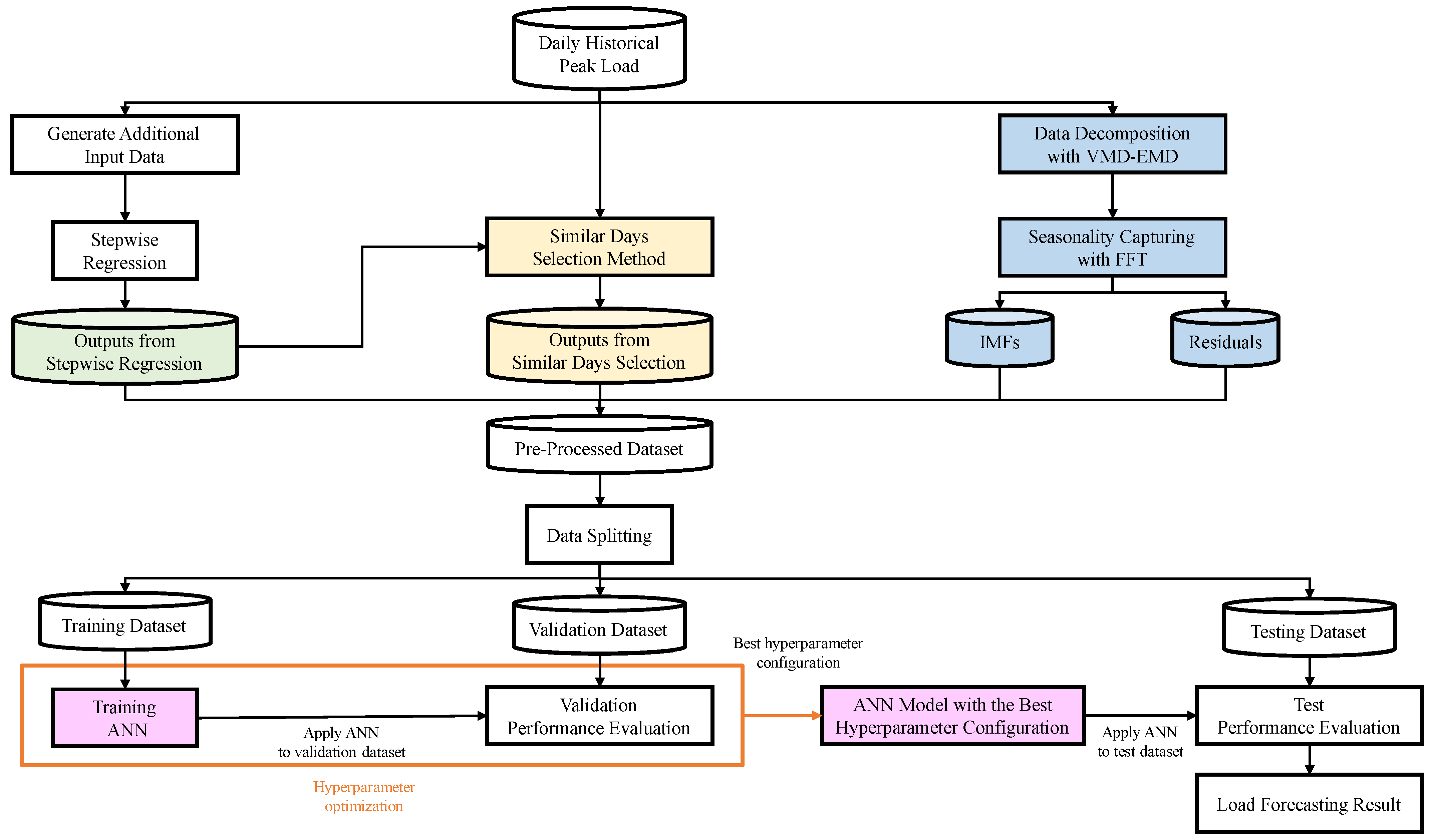
2.1. Architecture of the Proposed Model

The architecture of the proposed model is presented in Figure 1. It consists of three parts, which are input variable selection, input data decomposition and seasonality capturing, and forecasting model using ANN.

The input variable selection is further divided into stepwise regression and the selection of similar days. The stepwise regression technique is a standard statistical modeling approach that is performed to select a set of significant input variables from additional generated input data, while the similar days selection method is developed to select the days that are relatively similar to the target date to forecast the peak load. In the similar days selection method, similarity between two dates is measured using a weighted K-dimension Euclidean distance, where the K dimensions are significant variables from the stepwise regression and the weight for each variable is its coefficient in the regression model. In other words, the K dimensions of input variables used in the distance calculation are screened by stepwise regression to reduce the computational cost of the forecasting model. In the data decomposition and seasonality capturing part, historical data is decomposed using the VMD-EMD. Then, seasonal factors are measured and captured using the FFT.

Outputs from the first two parts include a screened dataset containing significant input variables, peak loads of the similar days, and IMFs and residuals from the VMD-EMD and FFT techniques. These outputs are used as the pre-processed dataset for training the forecasting model (ANN) in part three. The pre-processed dataset is split into training, validation, and testing datasets. First, an ANN is trained using the training dataset. Then, the validation dataset is applied to the trained ANN model for hyperparameter tuning. In hyperparameter tuning, the learning procedure is repeated until the model performance reaches the optimal point. After the best hyperparameter configuration is found, the tuned ANN model is tested with the unseen testing dataset to check for model overfitting and to evaluate the model’s forecasting performance.

The proposed model is constructed to have high forecasting performance, while reducing the computational cost of the forecasting model. High performance of the model is achieved by training the model with denoised data that present clear seasonality and trends and with the peak load of highly similar dates selected from the similar days selection method. The neural network structure and its computational cost can be reduced by training the model only with the significant variables selected from stepwise regression. In addition, the proposed similar days selection method has the ability to handle both normal days (defined as weekdays and weekends that are not special holidays in this paper) and special holidays, which makes the forecasting model more suitable to apply in a real situation. Moreover, the bias caused by hyperparameters can be prevented by applying the hyperparameter optimization technique. The bias in testing process from imbalanced number of normal days and special holidays in testing dataset can be avoided by taking their equal sample sizes. With the combination of the methods mentioned above, the proposed model can produce highly accurate forecast values, as well as reduce the complexity and computational cost. The concepts of data preparation, input variable selection, data decomposition and seasonality capturing, and ANN are presented in Section 2.2, Section 2.3, Section 2.4, and Section 2.5 respectively.

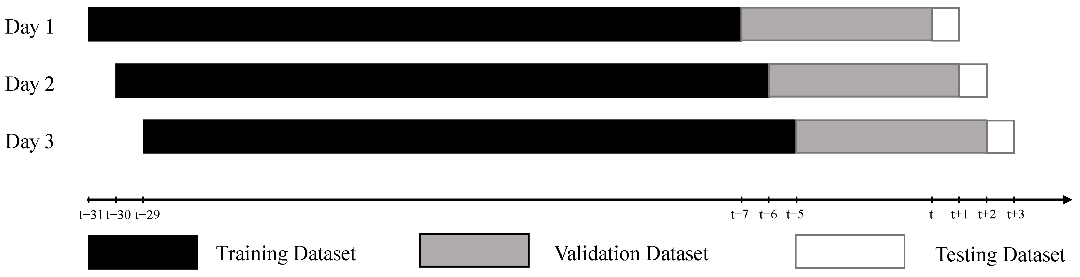
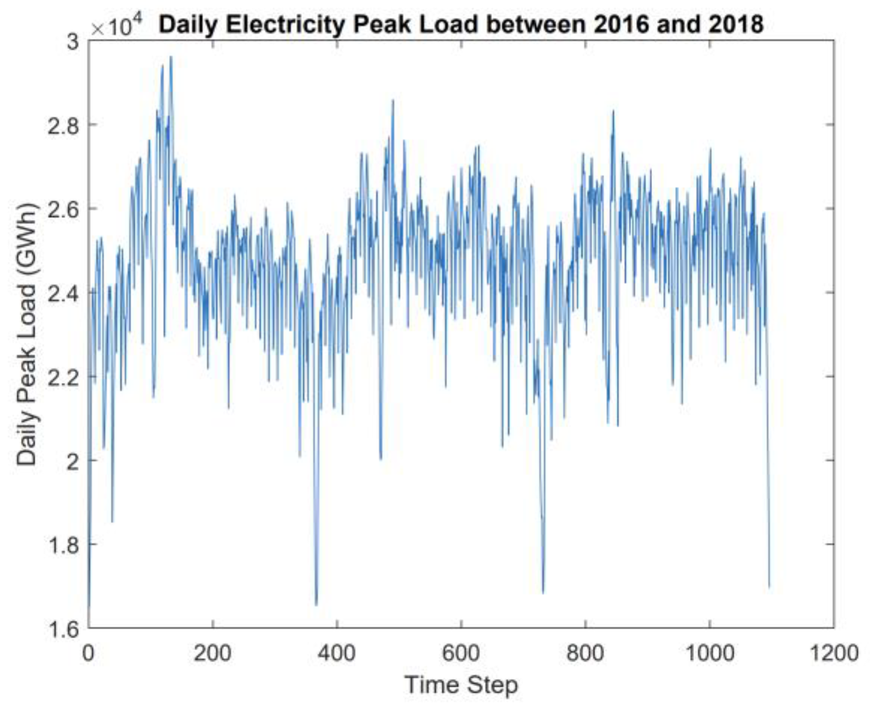
2.2. Data Preparation

In this study, Thailand’s electricity generation network is used as a case study to evaluate the efficiency of the forecasting model. Daily peak load in megawatts (MW) from January 2016 to December 2018 are used as raw input data. According to data separation theory, it is a common practice to divide the time series data into training, validation, and testing datasets [46]. This study uses variables that are derived from daily peak loads of 31 days before the target forecast date as a training dataset to let the model learn the patterns that appear in the historical data. To validate the performance of the forecasting model, 7 days before the forecasting target date is used as a validation dataset while keeping the target forecast date as a testing dataset.

To comprehensively validate the accuracy of the proposed model under various patterns of the peak load, the target forecast dates are selected by taking samples from the normal days and special holidays of the testing dataset. The samples are used to construct the forecasting model, instead of using all days in the testing dataset, to reduce the computational cost and to guide the forecasting model to learn the data patterns from normal days and from special holidays in a balanced manner. To achieve this balance, the number of the selected normal day is set as equal to the total number of special days in a year. In other words, taking equal sample sizes from normal days and special holidays can avoid bias in the testing process caused by a large number of normal days relative to the number of special holidays. The number of days of the week (Mon to Sun) is also equally selected. In each month, one day is randomly selected as the target forecast date first. Then, for the months that contain 31 days, one additional target forecast date is randomly selected. The criterion for assigning one day or two days is set based on the number of days in the month. The process of randomly selecting the forecasted target date is shown in Figure 2.

The pattern of electricity peak load fluctuates and continuously changes over time. To make the forecasting model adapt to each change, one-day-ahead forecasting is assigned for every target date in the testing dataset. To simulate a real situation, walk-forward testing (or sliding windows testing) is used to test the robustness of the model. In the walk-forward testing, the data is divided into training, validation, and testing datasets that contain overlapping data. Each dataset is selected by rolling forward through the time series as shown in Figure 3. Although this testing process is a time-consuming process due to the frequency of the retained data, the strength of this process is the adaptability, when the pattern of electricity peak load changes, which makes the walk-forward testing suitable to apply in a real situation [46].

2.3. Input Variable Selection

2.3.1. Additional Input Data Generation

First, the raw dataset containing two variables, date and peak load, from EGAT is processed to generate additional input data for the stepwise regression. The generated additional input variables are candidate input variables to be selected by stepwise regression. The generated inputs are binary indicator variables for day-of-the-week (Mon to Sun) and weekends, historical daily peak load with the lagged value from one day ($y_{t-1}$) to 10 days ($y_{t-10}$), lagged daily peak to moving average weekly and monthly index (${LPI}_t\left(L\right)$), and moving average ($MA\left(Q\right)$), starting from $\mathit{MA}\left(2\right)$ to $\mathit{MA}\left(7\right)$. The mathematical expression to compute ${LPI}_t\left(L\right)$ and $MA\left(Q\right)$ are as follows:

$${LPI}_t\left(L\right)=\frac{y_t}{\raisebox{1ex}{$\left({\sum }_{t=1}^L{y}_t\right)$}\!\left/ \!\raisebox{-1ex}{$L$}\right.}$$

(1)

$$MA\left(Q\right)=\frac{{\sum }_{q=1}^Q{y}_{t-q}}{Q}$$

(2)

where ${LPI}_t$(L) is lagged daily peak to moving average index, $y_t$ represents daily peak load at period t, L is length of the day, which is set equal to 7 days and 30 days, when considering the weekly LPI and monthly LPI, respectively, q is number of lagged period, and $Q$ is length of the day, which is set equal to 2 days and 7 days, when considering the two-days MA and weekly MA, respectively.

2.3.2. Stepwise Regression

Regression analysis is a popular and powerful statistical method used for measuring the strength of the linear relationship between two or more variables and computing their associations. A high correlation score refers to a strong linear association between the response variable and the explanatory variables, while a low correlation indicates that the variables are weakly associated. A multiple regression model can be written as:

$$y={\beta }_0{+\beta }_1{x}_1{+\beta }_2{x}_2{+\dots +\beta }_M{x}_M+\epsilon ,$$

(3)

where y is the response variable, ${\beta }_i$ represents the regression coefficient parameters (i = 0, 1, …, M), $x_i$ represents explanatory variables (i = 1,2, …, M), $\epsilon$ is a random error component, and M represents total number of explanatory variables.

Stepwise regression is a technique used to improve the accuracy of the regression model [47]. This technique selects significant variables that are highly associated with the response variable by using p-value to measure statistical significance among the candidate input variables. The candidate variables in this study are the variables from generated additional input data process in Figure 1. The p-value for each candidate explanatory variable tests the hypothesis regarding its correlation with the response variable. If the correlation does not appear to be significant, then there is not enough association between the changes in the candidate input variables and the shifts in the response variable. There are three widely used approaches in stepwise regression. A forward selection starts with no variable in the model and then adds the variables one by one based on the most statistically significant until no variables can enter the model. Backward elimination starts with all candidate input variables in the model and then removes the least statistically significant variable one at a time until the remaining variables cannot be further removed. A bidirectional elimination is a combination of forward selection and backward elimination for the purpose of finding which variables should be included and excluded in the regression model [48]. In this study, bidirectional elimination is used to select the significant input variables to train the ANN and to compute the weights of the important factors to be used in the similar days selection method. The criteria in the bidirectional elimination are α-to-enter and α-to-remove, which are set to 0.1 in this study. In addition, to ensure that there are sufficient input data to fit the regression model, the amount of input data is set to 24 months of input data prior to the month of the target date.

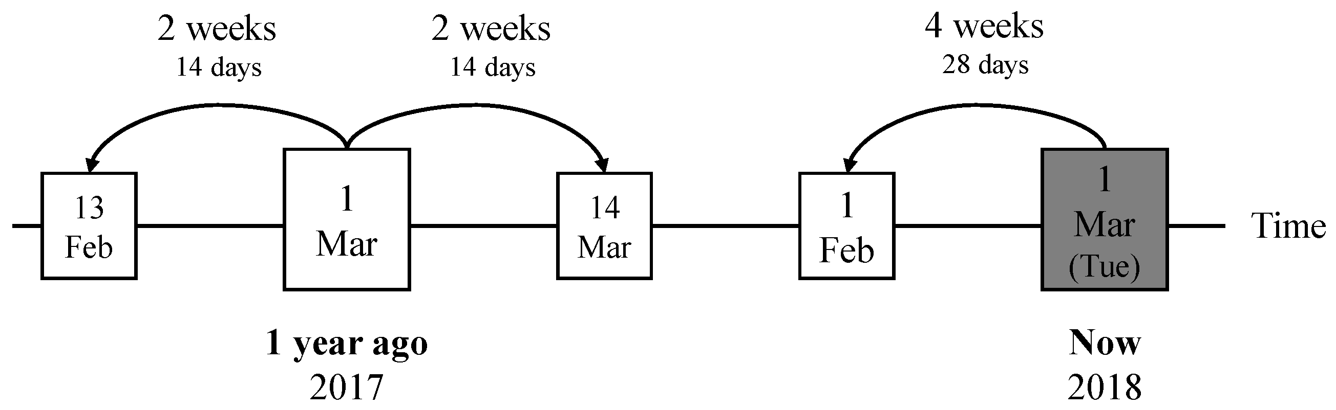
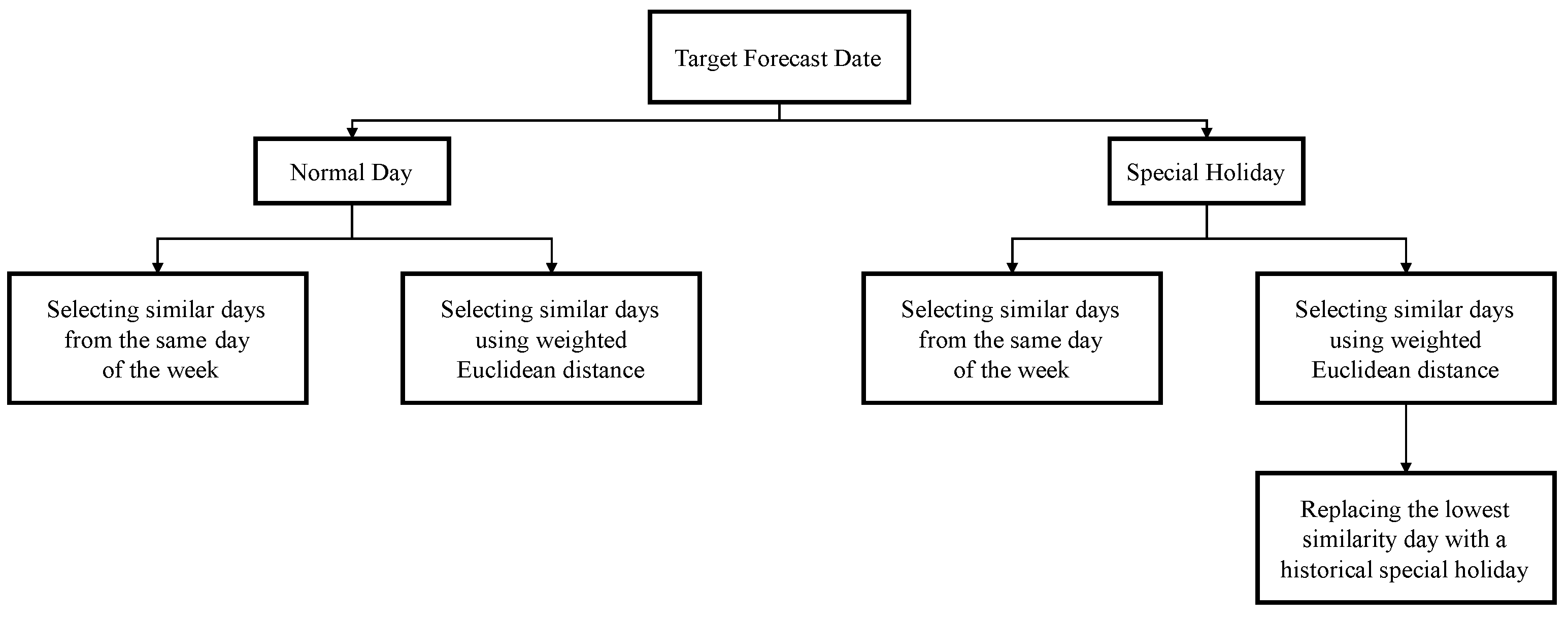
2.3.3. Similar Days Selection Method

Similar days selection method (SD) aims to find a set of dates that are similar to the target forecast date by searching through the historical data. This method selects a date based on the pattern of the daily peak load and then uses the daily peak load of the selected dates as input variables in the forecasting model. To perform similar days selection, the first step is to create a selection criterion. When creating the criterion, input variables and calculation processes for determining the selected input variables are considered [43].

This study uses a weighted n-dimension Euclidean distance as a criterion to measure the similarity among the daily peak load data of two different dates. This selection criterion interprets the similarity by using the concept of Euclidean distance, which is essential for utilizing evaluation [44]. The smaller the weighted Euclidean distance, the more similarity to the target date. Stepwise regression is used to select input variables for the similar days selection method to include only the input variables that are significantly associated with the response variable (i.e., daily peak of the target forecast date). The mathematical expression of the weighted n-dimension Euclidean distance is shown below:

$$WED=\sqrt{w_1{(\Delta P_1)}^2{+w}_2{(\Delta P_2)}^2{+\dots +w}_S{(\Delta P_S)}^2}$$

(4)

$$\Delta P_{i }{=P}_f-P_i ,$$

where WED is weighted Euclidean distance, $w_s$ represents the weighted of selected variable s from the stepwise regression, S represents total number of the selected variable, and $\Delta P_i$ represents the difference between the values of a variable of the target forecast date ($P_f$) and variable of the historical date ($P_i$).

The range of input days used in the similar days selection model is set based on correlation. Since the past 1 month and the past 1 year from the target forecast date potentially have high correlations, the limits of the days used in the similar days selection model are set as shown in Figure 4. The input range is selected from the prior four weeks to the target date, and two weeks before and after the target day in the previous year.

The appropriate number of selected days is an important research question of the similar days selection problem. When considering weighted Euclidean distance, there are many days that can be selected as the day that is similar to the target forecast date since the weighted Euclidean distance is low. To answer this question, this study proposes the criterion for determining the number of the selected days called one-year weighted average of the largest jump in seven days. The steps of the criterion are as follows:

• For a given target forecast date, rank the weighted Euclidean distance (WED) from minimum to maximum;
• Find the difference in the WED between the day with adjacent ranks in the top n days that have the lowest WED;
• Find the largest jump (largest difference) among the differences from Step 2 in the top n days. The number of selected days is the number of days before the occurrence of the largest jump;
• Repeat Steps 1 to 3 for a year (365 target dates). After completing this step, there are 365 values of the number of selected days;
• Find the frequency d_i for each possible value of the number of selected days, i = 1, 2, …, N;
• Calculate the weighted average number of selected days, $\overline{W}$, using Equation (5);
• Each value for the number of selected days has the weight $w_i$ that can be computed according to Equation (6).

$$\overline{W}=\frac{{\sum }_{i=1}^N{(d}_i{\ast w}_i)}{{\sum }_{i=1}^N{w}_i },$$

(5)

$$w_i=\frac{d_i}{{\sum }_{i=1}^N{d}_i },$$

(6)

where $\overline{W}$ is the weighted average of the number of selected days, $w_i$ represents the weight of $d_i$, and N is the possible number of selected days.

The historical data of daily peak load, day of the week, weekend, and lagged daily peak to moving average index LPI are used as the variables in the similar days selection method. However, the historical peak load has a very large value compared to the other variables in the input data. This issue makes the selection model neglect the significant variables that affect the performance of the similar days selection. As a result, the selection model becomes ineffective, especially when applied to special holidays. To resolve the issue, this study proposes a new similar days selection criterion that considers three variables, including historical daily peak load, indicator variables for day of the week, and special holidays, as shown in Figure 5.

When the target forecast date is a normal day, similar days are selected using weighted Euclidean distance and day of the week indicator. The weighted Euclidean distance measures the similarity of the peak load between the target date and another candidate date, while the day of the week indicator measures whether the candidate date has the same day of the week as the target date. For example, if the target forecast date is Tuesday, 1 March 2018, the candidate date will be selected from four Tuesdays from the prior four weeks, and two Tuesdays from two weeks before and after the target day in the previous year as shown in Figure 4. On the other hand, when the target forecast date is a special holiday, the last day of the selected similar days, $\overline{W}$, based on weighted Euclidean distance, is replaced with the same special holiday in the previous year. For example, if the target forecast date is Christmas day, the last day of the selected similar day based on the weighted Euclidean distance will be replaced with the Christmas day of the previous year.

2.3.4. Numerical Example of Input Variable Selection

In the numerical example, the target date is Monday, 1 January 2018. The raw input dataset to the stepwise regression contains 24 months of input data prior to the month of the target date, i.e., peak load from 1 January 2016 to 31 December 2017. After generating additional input data including binary indicator variables for day-of-the-week (Mon to Sun) and weekends, historical daily peak load with the lagged value from one day ($y_{t-1}$) to 10 days ($y_{t-10}$), lagged daily peak to moving average weekly and monthly index (${LPI}_t\left(L\right)$), moving average ($MA\left(Q\right)$) MA, lagged peak load, and LPI, the stepwise regression is then performed for all target dates in January 2018 with α-to-enter and α-to-remove of 0.10. Note that as the target date moves to a new month, input data are updated and a new stepwise regression is refit. The final model from stepwise regression of January 2018 is shown in Equation (7). The coefficients of significant variables in the regression model are used as weights in the calculation of weighted Euclidean distance (Equation (4)).

Table 1. Example of computing weighted Euclidean distance for = weekend indicator variable.

Target Date $\left({\mathit{P}}_{\mathit{f}}\right)$	No. $\left(\mathit{i}\right)$	Past Date $\left({\mathit{P}}_{\mathit{i}}\right)$	${\left(\mathbf{\Delta }{\mathit{P}}_{\mathit{k}}\right)}^2$ $={{(\mathit{P}}_{\mathit{f}} {- \mathit{P}}_{\mathit{i}})}^2$	${\mathit{w}}_{\mathit{k}}{\left(\mathbf{\Delta }{\mathit{P}}_{\mathit{k}}\right)}^2$	WED
1 January 2018	1	1 January 2017 (Weekday)	0	0	0
(Weekday)	2	2 January 2017 (Weekday)	0	0	0
	3	3 January 2017 (Weekday)	0	0	0
	4	4 January 2017 (Weekday)	0	0	0
	5	5 January 2017 (Weekday)	0	0	0
	6	6 January 2017 (Weekend)	1	993	31.51
	7	7 January 2017 (Weekend)	1	993	31.51

shows the example for computing the weighted Euclidean distance of the indicator variable “Weekend”. The weekend indicator is set equal to zero for weekdays and one for weekends. In Table 1, a date with low WED means that the date is relatively similar to the target forecast date, i.e., the first five dates in Table 1 are exactly similar, WED = 0, to the target date with respect to weekend indicator, while the last two dates are not the same.

The number of the selected similar days is defined using a criterion based on one-year weighted average of the largest jump in N = 7 days.

Table 2. Example of finding the largest jump in seven days.

Target Date	No.	Generated Additional Dates	WED (Ranked)	WED Difference
1 January 2018	1	3 January 2017	584.77	-
	2	31 December 2016	1135.79	551.02
	3	1 January 2017	1190.57	54.78
	4	2 January 2017	1196.36	5.79
	5	30 December 2017	1541.40	345.04
	6	31 December 2017	1595.00	53.60
	7	29 December 2017	2020.71	425.72

shows the example for finding the largest jump that occurs in seven days. First, the candidate dates are ranked ascendingly using their WED. The largest jump is the largest difference between the two adjacent candidate dates (after ranking). Thus, in this example, the largest jump occurs after the first day. After computing the largest jump of all target dates for the whole year, frequency ($d_i$), weight ($w_i$) of each possible number of days prior to the largest jump, and the weighted average number of selected similar days $\overline{W}$ are computed, as shown in

Table 3. Example of computing one-year weighted average of the largest jump in seven days.

Number of Days until the Biggest Jump Occurs	1 Day	2 Days	3 Days	4 Days	5 Days	6 Days	7 Days
$d_i$	133	70	48	38	20	33	23
wi	0.36	0.19	0.13	0.10	0.05	0.09	0.06
$\overline{W}$	2.823 ≅ 3

. In this example, $\overline{W}$ is approximately three days; therefore, the number of similar days is set to three.

Finally,

Table 4. Example of the new similar days selection criterion.

Target Date		1 January 2018 (Mon) (New Year’s Day)
Similar day selected from the same day of the week	SD1	25 December 2017 (Mon)
	SD2	18 December 2017 (Mon)
	SD3	11 December 2017 (Mon)
	SD4	4 December 2017 (Mon)
	SD5	19 December 2016 (Mon)
	SD6	26 December 2016 (Mon)
	SD7	2 January 2017 (Mon)
	SD8	9 January 2017 (Mon)
Similar day selected based on WED	SD9	3 January 2017
	SD10	31 December 2016
	SD11	1 January 2017 (previous New Year’s Day)

contains 11 similar days to the target date in this example. The first eight days (SD1–SD8) are the days that have the same day of the week indicator as the target forecast date. Three additional similar days are selected based on the weighted Euclidean distance (SD9–SD11). In the example, the target forecast date is a special holiday (New Year’s Day 2018), thus the lowest similarity day (SD11) based on the weighted Euclidean distance is replaced with the same special holiday of the previous year (New Year’s Day 2017).

$$\begin{array}{c}{y}_t{=4414+1178 Mon}_t{ + 508 Tue}_t{ + 502 Fri}_t{ + 674 Sat}_t{ - 478 Sun}_t{ - 993 Weekend}_t{- 2243 LPI}_t\left(30\right)+0.7612 \\ y_{t-1} + 0.061 y_{t-2}+0.1148 y_{t-6}+0.2105 y_{t-7} ,\end{array}$$

(7)

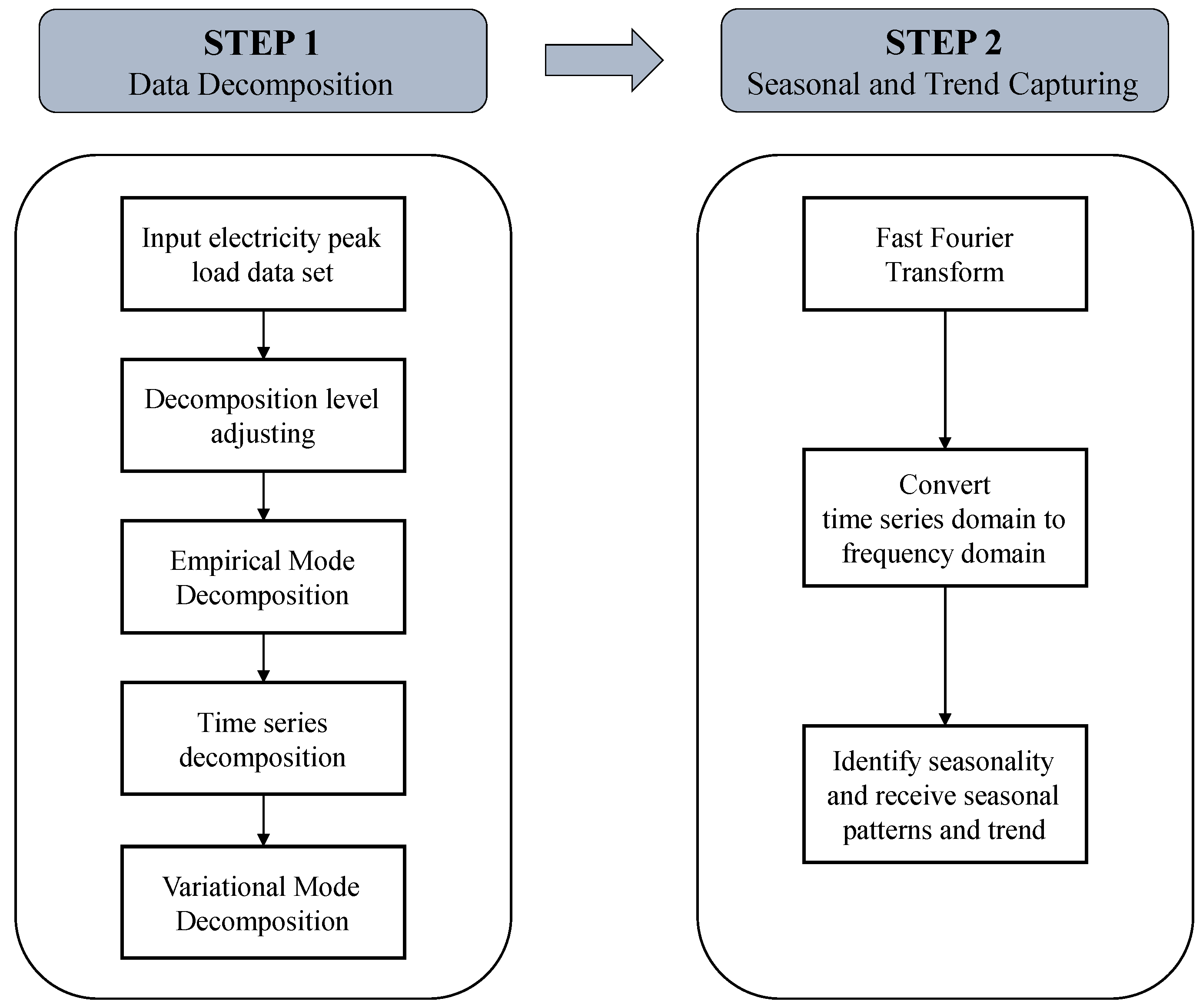
2.4. Data Decomposition and Seasonality Capturing

In the first phase, the original electricity peak load is clouded with uncontrolled noise components. Too much noise in the time series can dominate the forecasting accuracy caused by volatility and randomness [28]. To eliminate redundant noise and identify seasonality patterns, data decomposition and seasonality capturing are applied to the original data as shown in Figure 6. VMD is applied to make the original data smoother by separating the non-linear and non-stationary parts out of the time series. VMD has a problem with nonautomated decomposition level adjustment. To solve this problem, EMD is used as a guide to adjust the decomposition level of VMD due to its ability to auto-adjusted decomposition level. After performing the noise elimination process, FFT is applied to identify and capture seasonality and trend that are left in the denoised series. The description of VMD-EMD and FFT are presented in Section 2.4.1 and Section 2.4.2.

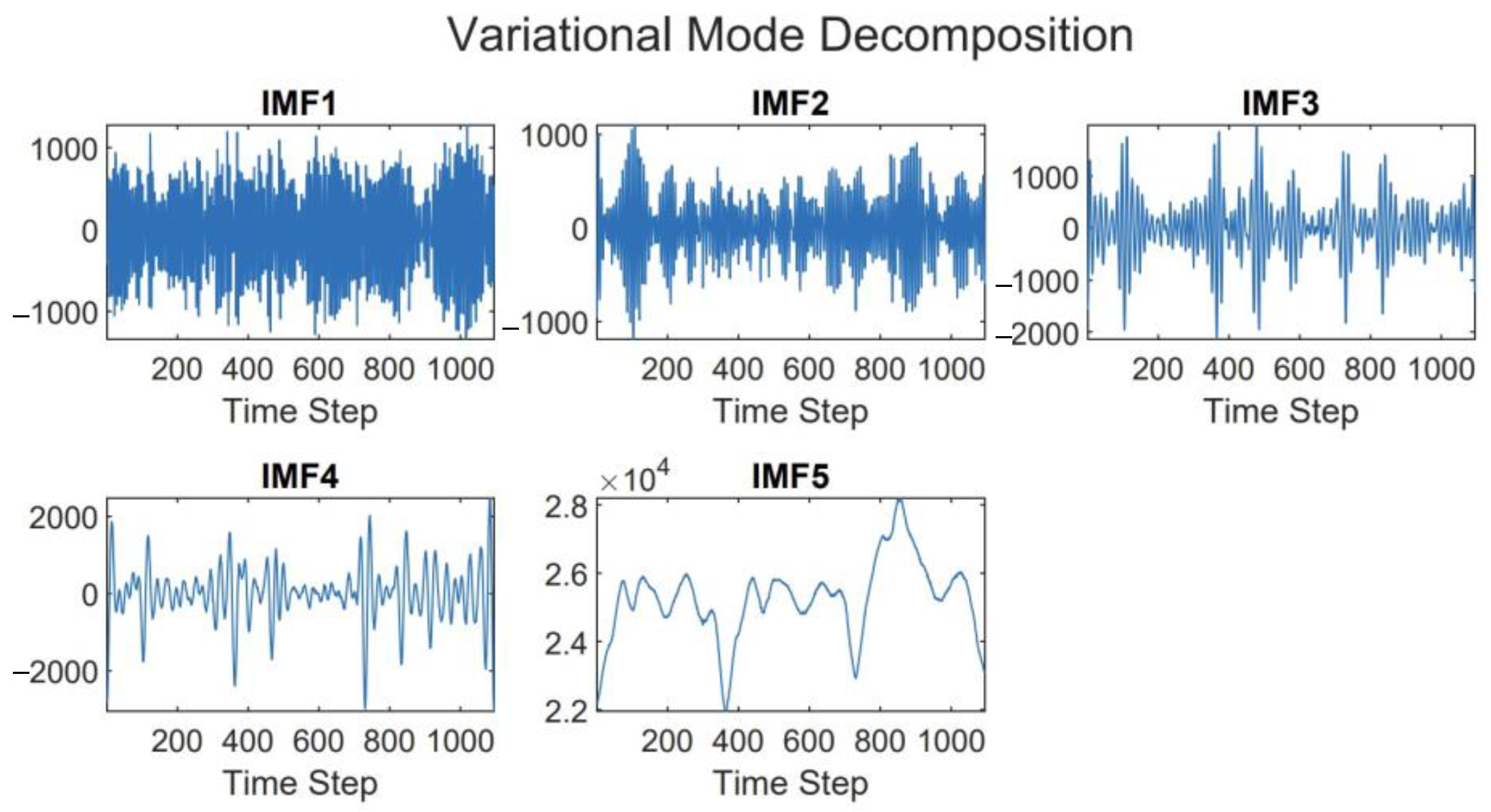
2.4.1. Variational Mode Decomposition

Variational mode decomposition (VMD) is a self-adaptive signal processing that is used to eliminate noise from the original time series data. It is capable of separating non-linear and non-stationary data by decomposing the data into intrinsic mode functions (IMFs) and residuals. Unlike the traditional EMD method, VMD solves the mode mixing problem and improves its reliability by shifting from the sifting process approach to the alternating direction method of the multipliers approach [49].

In the VMD technique, each mode is assumed to be an infinite bandwidth with unique center frequencies [50]. The steps for obtaining the bandwidth of each mode are as follows:

• In each mode (u_k), the Hilbert transform is applied to obtain a unilateral frequency spectrum that is computed from its analytical signal;
• Estimate the center frequency by applying an exponential turned to shift the model’s frequency spectrum to the baseband;
• Compute the bandwidth of each mode by applying the optimal-solution processing based on Gaussian smoothing. The mathematical expression of the constrained variational problem is as follows:

$${\mathrm{m}\mathrm{i}\mathrm{n}}_{u_k{w}_k}\left\{{\sum }_{k=1}^K\Vert {\partial }_t\left[\left(\delta \left(t\right)+\frac{j}{\mathsf{\pi }t}\right){\ast u}_k\left(t\right)\right]e^{{-jw}_{k}t}{\Vert }_2^2\right\},$$

(8)

$$\mathrm{s.t.} {\displaystyle \sum }_{k=1}^K{u}_k=f\left(t\right),$$

where δ_t is the Dirac distribution, t and k represent the time index and the number of decompositions, {u} = {u₁, …, u_k} refers to the set of modal functions, and {w} = {w₁, …, w_k} refers to the center frequencies after decompositions.

4.

To convert the constrained variational problem above into an unconstrained variation problem, the penalty term (α) and the Lagrange multiplier, λ(t), are applied to the model as follows:

$$\begin{array}{c}L\left(u_k{w}_k\lambda \right)=\alpha {\displaystyle \sum }_{k=1}^K\Vert {\partial }_t\left[\left(\mathsf{\delta }\left(t\right)+\frac{j}{\mathsf{\pi }t}\right){\ast u}_k\left(t\right)\right]e^{{-jw}_{k}t}{\Vert }_2^2\\ \Vert +f\left(t\right)-{\displaystyle \sum }_{k=1}^K{u}_k\left(t\right){\Vert }_2^2+\langle \lambda \left(t\right),f\left(t\right)-{\displaystyle \sum }_{k=1}^K{u}_k\left(t\right)\rangle \end{array}$$

(9)

5.

To find the optimal solution of the problem, the saddle point of the enlarged Lagrange function is obtained from the Alternate Direction Method (ADM) as follows:

$${\mathrm{Min}: \hat{u}}_k^{n+1}=\frac{\hat{f}\left(w\right)-{\sum }_{i\ne k}\hat{u}\left(w\right)+\hat{\lambda }(w)/2}{{1+2\alpha (w-w}_k{)}^2},$$

(10)

$${\mathrm{Min}: w}_k^{n+1}=\frac{{\int }_0^{\infty }w{\left|{\hat{u}}_k^{n+1}\left(w\right)\right|}^{2}dw}{{\int }_0^{\infty }{\left|{\hat{u}}_k^{n+1}\left(w\right)\right|}^{2}dw},$$

where n is the iteration number, and $\hat{f}\left(w\right)$, ${\hat{u}}_i\left(w\right)$, $\hat{\lambda }(w)$, and ${\hat{u}}_k^{n+1}$(w) represent the Fourier transforms of f(t), u_i(t), λ(t), and $u_k^{n+1}$(t), respectively.

Decomposition level adjusting is the open problem of VMD that many researchers attempt to solve. The excessive number of decomposition levels can cause mode aliasing problems and bring out additional noise, while lacking the number of IMFs will make the original data become under-decomposed. To avoid trial and error and save time in the optimization process, the advantage of the auto-adjusted decomposition level from EMD is used. Thus, the problem of determining a suitable decomposition level of VMD can be solved by using EMD as a guide.

2.4.2. Fast Fourier Transform

Fast Fourier Transform (FFT) is a popular and powerful transformation analysis. It is used to convert the time series domain to the frequency domain and clearly show the individual frequency and the dominant frequency [51]. When seasonality is hidden in the time series, FFT is considered to be an effective method that has the ability to identify seasonality behind the time series.

Historical electricity peak load is the time series dataset that consists of complex patterns affected by the seasonal component. To improve the forecasting performance, the effective way is to train the forecasting model with the transformed time series rather than the original time series. With the identification capability of FFT, this study uses FFT to identify and capture seasonality and trend behind the electricity peak load and use the transformed data as a set of additional variables to train the forecasting model.

2.5. Artificial Neural Network

Artificial neural network (ANN) is a machine learning model that mimics the massively parallel computations in the brain and has the capability for solving complex problems [52]. ANN can show its capability in complex control, classification, and recognition tasks and is effective in recognizing patterns and making simple rules for complex problems.

The most common ANN model is called the multi-layer feedforward neural network (MLFN). The model consists of two different phases, which are the training phase or learning phase and the execution phase. In the training phase, ANN is trained by specific input data to return a specific output. For the execution phase, ANN returns output based on the input foundation. MLFN contains three fundamental layers which are the input layer, one or more hidden layers, and the output layer. The input layer contains neurons and each neuron is multiplied by its adjustable weight. Then, the inputs that combine their weights are sent to a non-linear transfer function inside the hidden layer for computing output and sent out to the output layer. The summarized mathematical equation of the MLFN with one hidden layer is shown below:

$$y=f°\left({\displaystyle \sum }_{j=1}^J{W}_j{f}_j^h\left({\displaystyle \sum }_{i=1}^I{W}_{ij}{x}_i\right)\right),$$

(11)

where y is the output, $f°$ and $f_j^h$ are transfer functions of the output node and hidden node $j$, respectively, J denotes the number of hidden nodes, $x_i$ is the input data of input node i, I is the number of input nodes, $W_{\mathit{ij}}$ is the adjustable weight from the input node i to hidden node j, and $W_j$ is the adjustable weight from hidden node j to the output node.

3. Results

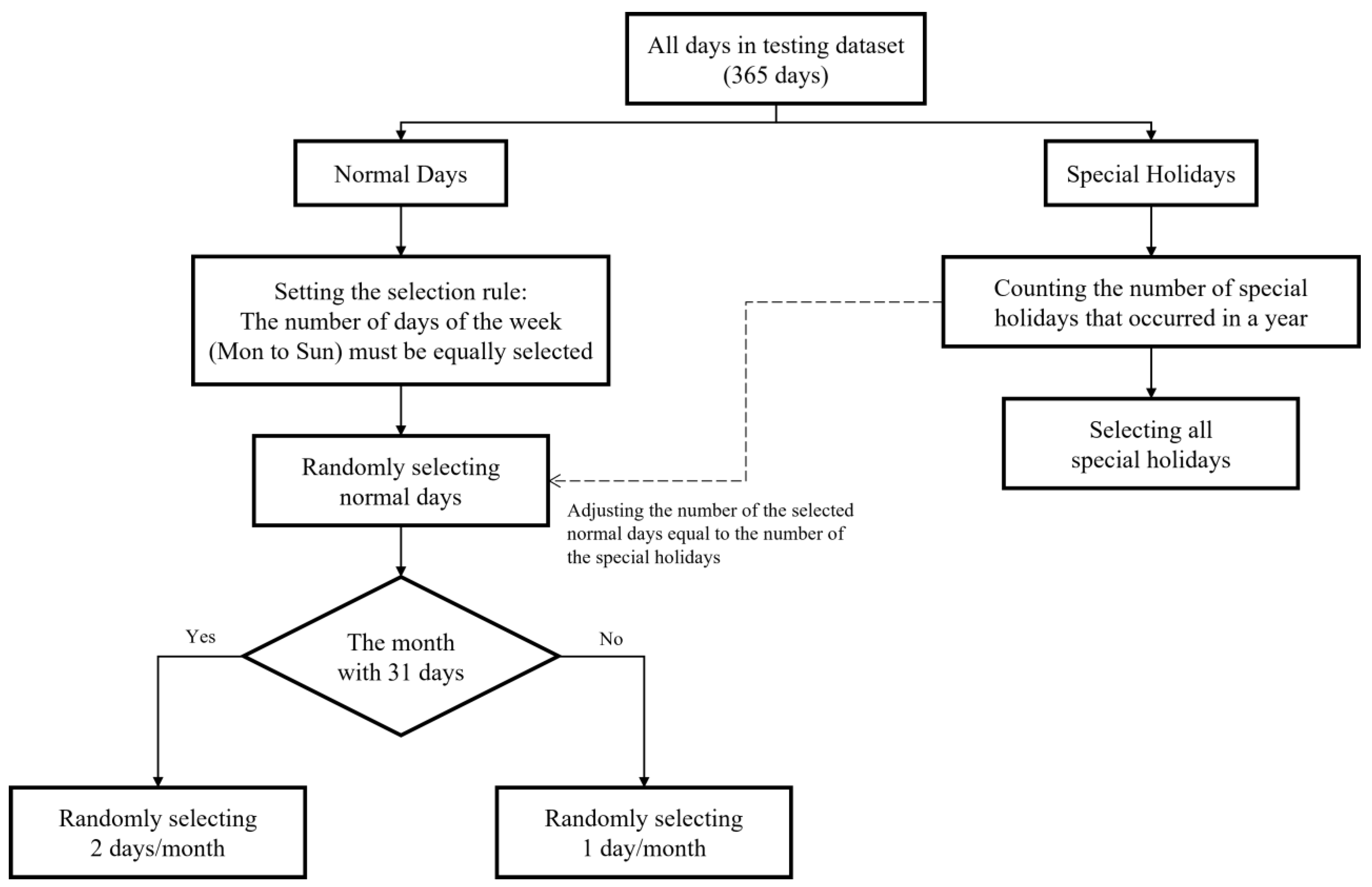
3.1. Target Forecast Date

This study selects the target forecast dates by taking samples from the days in the year 2018. To balance the learning process of the forecasting model, the number of the selected normal days is set equal to the number of special days. There are 19 special days in 2018. Thus, 19 normal days are randomly selected, and the total forecasted days, $N$, is equal to 38 days. According to the selection criterion for selecting normal days, two normal days are assigned to the months with 31 days (Jan., Mar., Jul., Aug., Oct., and Dec.) and one normal day is assigned to the other months. The randomly selected days used as the target forecast date are shown in

Table 5. List of the selected target dates used in the experiment.

Month	Target Dates
	Normal Day		Special Day
Jan.	22 January 2018 (Mon.)	27 January 2018 (Sat.)	1 January 2018 (New Year’s Day)
Feb.	20 February 2018 (Tue.)
Mar.	7 March 2018 (Wed.)	25 March 2018 (Sun.)	1 March 2018 (Makha Bucha Day)
Apr.	12 April 2018 (Thu.)		6 April 2018 (Chakri Day)	13 April 2018 (Songkran)	14 April 2018 (Songkran)	15 April 2018 (Songkran)
May	21 May 2018 (Mon.)	18 May 2018 (Fri.)	1 May 2018 (Labor Day)	4 May 2018 (Coronation Day)	14 May 2018 (Farmer’s Day)	29 May 2018 (Visakha Bucha Day)
June	16 June 2018 (Sat.)
Jul.	10 July 2018 (Tue.)	15 July 2018 (Sun.)	27 July 2018 (Asarnha Bucha Day)	28 July 2018 (King’s Brithday)	28 July 2018 (Buddhist Lent Day)
Aug.	20 August 2018 (Mon.)	1 August 2018 (Wed.)	12 August 2018 (Mother’s Day)
Sep.	11 September 2018 (Tue.)
Oct.	10 October 2018 (Wed.)	25 October 2018 (Thu.)	13 October 2018 (Memorial Day)	23 October 2018 (Piyamaharaj Day)
Nov.	22 November 2018 (Thu.)
Dec.	14 December 2018 (Fri)	8 December 2018 (Sat.)	5 December 2018 (Father’s Day)	10 December 2018 (Ratthathammanoon Day)	31 December 2018 (New Year’s Day)

.

3.1.1. Input Variables Selection

After applying stepwise regression, the significant input variables selected from stepwise regression include day of the week indicator variables (Mon., Tue., Fri., and Sun.), weekend indicator variable, weekly LPI, and historical daily peak load with the lags of one, two, six, and seven days (T − 1, T − 2, T − 6, and T − 7). The lists of generated additional input variables and the significant variables from stepwise regression are shown in

Table 6. The lists of generated additional input variables and the significant input variable.

Variable Type	Generated Additional Input Variable	Significant Input Variable
Day of the week indicators	Mon., Tue., …, Sun. (7 variables)	Mon., Tue., Fri., Sun. (4 variables)
Weekend indicator	0, 1 (2 variables)	0, 1 (2 variables)
Historical peak load	T − 1, T − 2, …, T − 10 (10 variables)	T − 1, T − 2, T − 6, T − 7 (4 variables)
LPI	Weekly LPI, Monthly LPI (2 variables)	Weekly SI (1 variable)
MA(L)	MA(2), MA(3), …, MA(7) (6 variables)	None

.

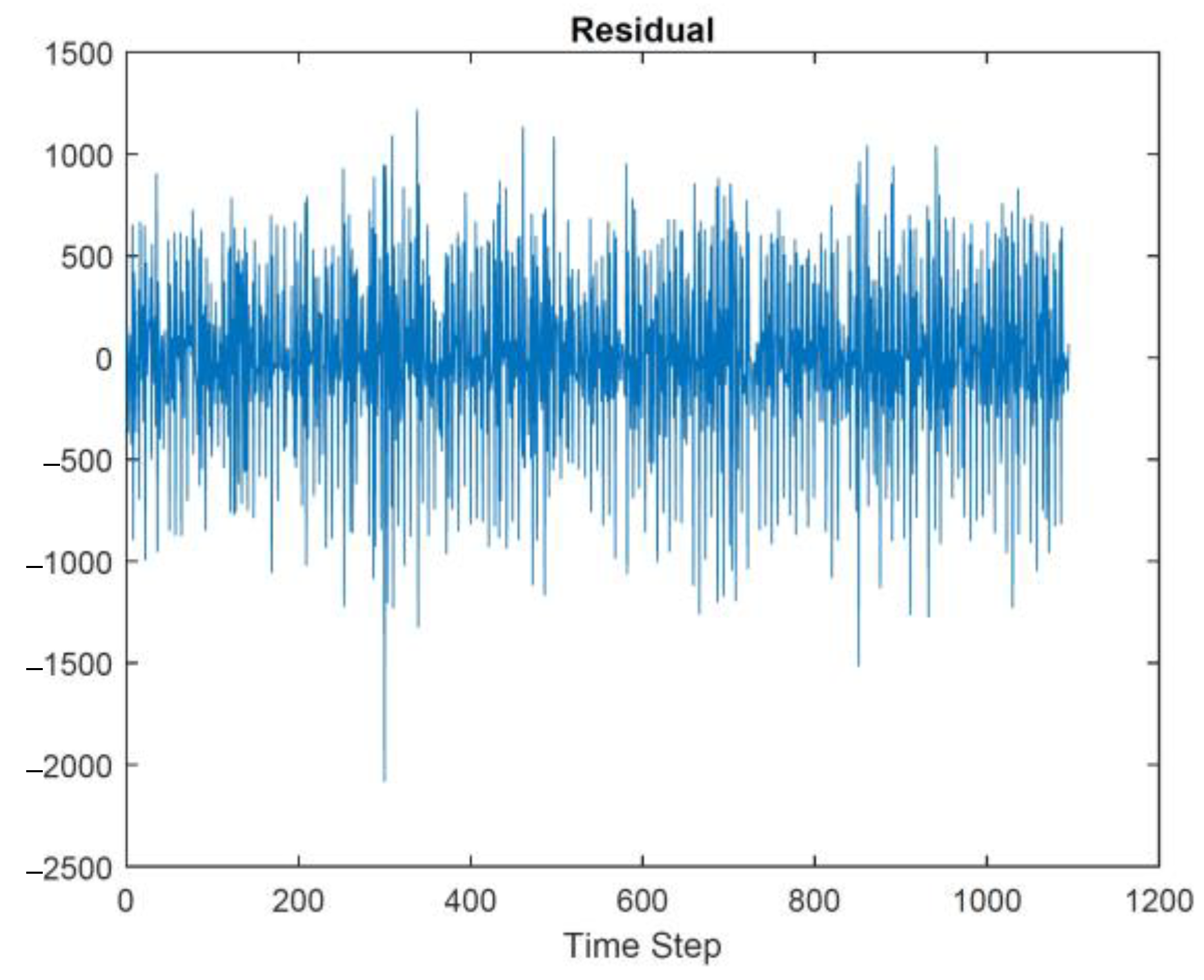
3.1.2. Data Denoising

Real electricity daily peak load data provided by EGAT from 2016–2018 are used as the experimental dataset. The original data contains 1096 observations as shown in Figure 7. The original electricity peak load shows the complex pattern related to non-linear and non-stationary parts. When using VMD, the original time series is decomposed into k IMF. The number of k represents the decomposition level of VMD that is determined by the guide from EMD. After applying EMD to the dataset of the case study, it suggests that the value of k is equal to five. MATLAB software is used for performing VMD. The other factors used in VMD are set as the default values of MATLAB software. The maximum number of optimization iterations and penalty level is set equal to 500 and 1000, respectively, while peaks are used as the method to initialize the central frequencies. The results after decomposition into five-level IMFs and residuals are shown in Figure 8 and Figure 9, respectively. Figure 8 shows the decomposition components from the highest frequency to the lowest frequency starting from IMF1 to IMF5. IMF4 and IMF5 show low-frequency signals with a strong vibration that reflect the trend components captured from the original data. Contrasting with the remaining components, IMF1, IMF2, IMF3, and the residuals in Figure 9 show high-frequency signals with low constancy but significant fluctuation.

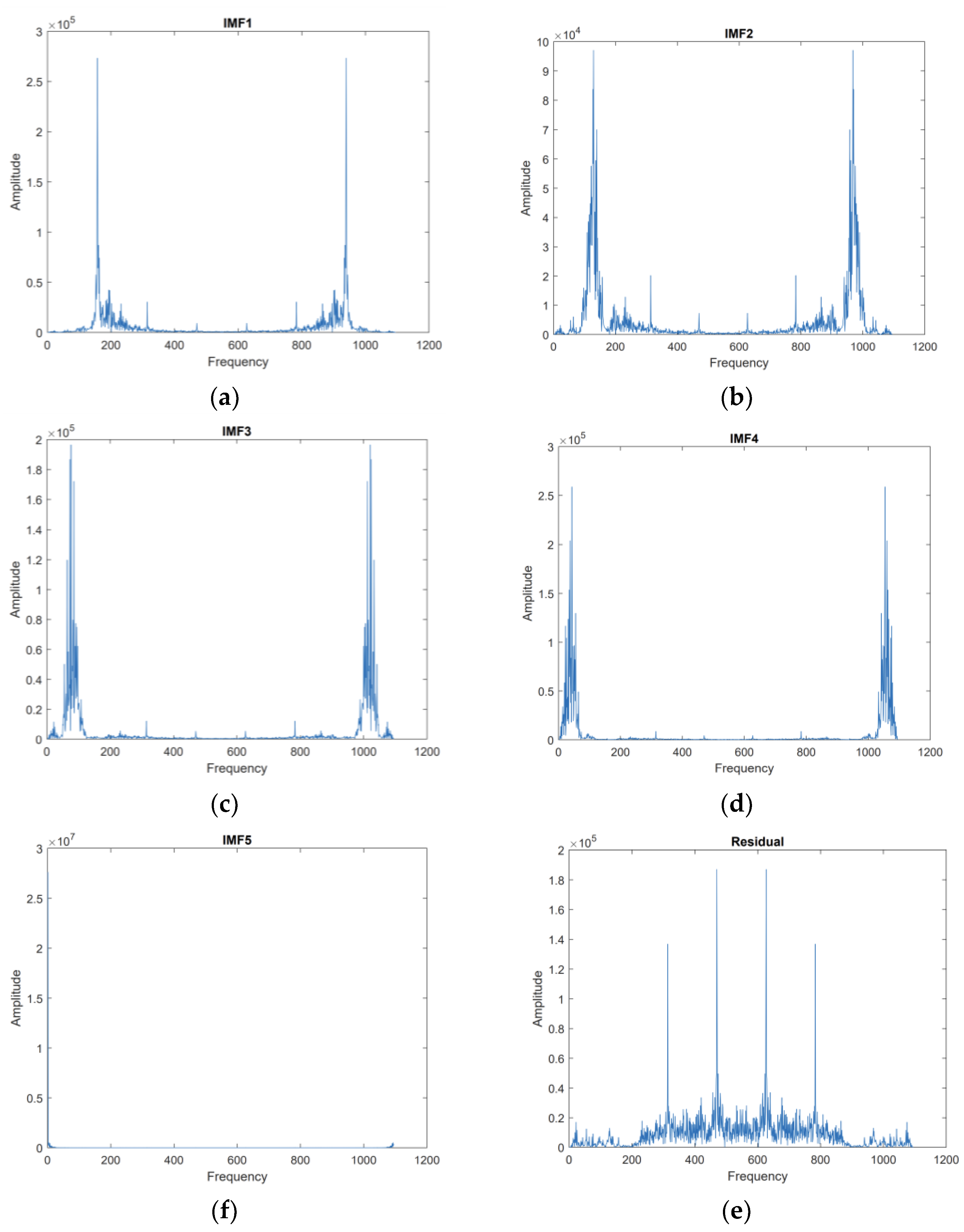
3.1.3. Seasonality and Trend Capturing

To capture the seasonality and trend components, FFT is applied to all IMFs and residuals. The resulting seasonality and trend components after applying FFT are clearer to identify and easier to capture, as shown in Figure 10.

3.2. Performance Measures

This study evaluates the forecasting performance of the models by using Mean Absolute Percentage Error (MAPE), Root Mean Square Error (RMSE), and Mean Absolute Error (MAE). MAPE is a measurement that does not depend on the unit of the forecasted data. It is adopted to explain the relative error RMSE and measures the difference between the predicted value and the actual value by presenting the error in terms of square root. MAE is another commonly used measurement of forecast errors in the time series problem. The mathematical expression of MAPE, MSE, and MAE are shown in Equation (12)–(14), respectively.

$$\mathrm{MAPE}=\frac{1}{N}{\sum }_{t=1}^N\frac{\left|\left(y_t{-\hat{y}}_t\right)\right|}{y_t}\times 100,$$

(12)

$$\mathrm{RMSE}=\sqrt{\frac{1}{N}{\sum }_{t=1}^N{\left(y_t{-\hat{y}}_t\right)}^2},$$

(13)

$$\mathrm{MAE}=\frac{1}{N}{\sum }_{t=1}^N\left|y_t{-\hat{y}}_t\right|,$$

(14)

where $y_t$ represents an actual electricity peak load in period t, ${\hat{y}}_t$ represents a forecasted electricity peak load in period t, and N represents a total number of forecasting periods.

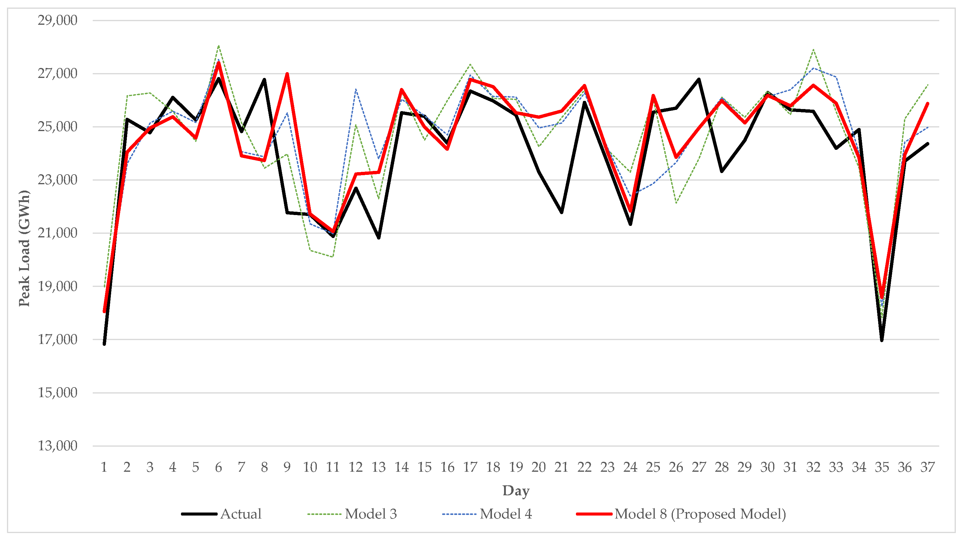
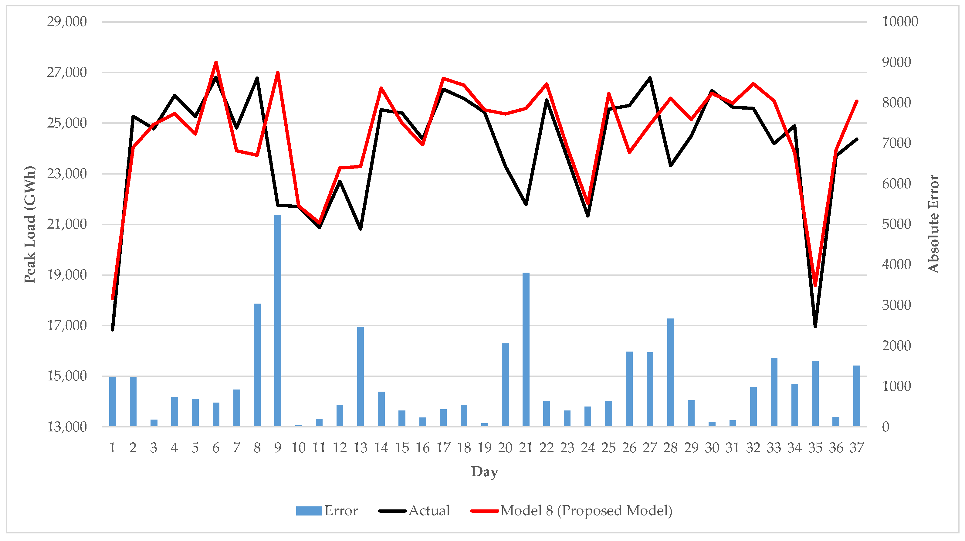
3.3. Experimental Results and Discussion

After applying the similar days selection method and data pre-processing method, significant variables from stepwise regression, daily peak loads of 11 days from the similar days selection method, and IMFs and residuals from data pre-processing are used as input variables of ANN. Eight experiments are conducted to evaluate the performance of the proposed model. The eight experiments contain all possible combinations of input variables. That is, all the input variables to the stepwise regressions, as well as only significant variables from the stepwise regression, may be used as one experimental factor. This is denoted as “all” and “stepwise.” In the case of inputs from similar days selection and VMD-EMD-FFT, the experiment is set with or without these methods in the model. The training, validation, and testing results of the eight experiments are shown in

Table 7. Results of the eight experiments when applying with training dataset.

Expr.	Stepwise	SD	VMD-EMD-FFT	Train			Validate			Test
				MAPE	RMSE	MAE	MAPE	RMSE	MAE	MAPE	RMSE	MAE
1	No	No	No	0.109%	33	26	0.066%	26	16	6.482%	1911	1498
2	No	Yes	No	0.063%	16	15	0.042%	16	10	6.523%	2035	1526
3	No	No	Yes	0.084%	27	20	0.062%	23	15	5.987%	1706	1408
4	No	Yes	Yes	0.067%	21	16	0.124%	18	27	5.257%	1626	1218
5	Yes	No	No	0.633%	259	150	0.366%	156	89	7.530%	2473	1717
6	Yes	Yes	No	0.073%	18	17	0.067%	25	16	6.324%	1949	1474
7	Yes	No	Yes	0.080%	21	19	0.068%	26	16	6.192%	1758	1423
8	Yes	Yes	Yes	0.069%	18	17	0.059%	23	14	4.894%	1593	1135

. However, before testing the forecasting model with the unseen dataset, the validation dataset is applied to optimize ANN hyperparameters that are suitable for each target forecast date. This means that the optimization process is performed every time when the target forecast date changes. This study uses grid search to optimize the hyperparameters of ANN with a single hidden layer. The grid search varies three hyperparameters, which are number of hidden nodes, training cycle, and learning rate. The optimization ranges of the hyperparameters are shown in

Table 8. The optimization range of ANN hyperparameter.

Hyperparameter	Optimization Range
Hidden node	1, 5, 10
Training cycle	50, 100, 500, 1000, 1500
Learning rate	0.1, 0.01, 0.001, 0.0001, 0.00001

.

Referring to the results in Table 7, comparisons between with and without VMD-EMD-FFT from four pairs of experiments (1 vs. 3, 2 vs. 4, 5 vs. 7, and 6 vs. 8) indicate that VMD-EMD-FFT can improve the performance of the forecasting model for all four comparisons, while the similar days selection method shows its strength only when VMD-EMD-FFT is applied to the model (i.e., experiments 3 vs. 4, and 7 vs. 8). Likewise, applying significant variables chosen from stepwise regression is effective only when the similar days method is performed (i.e., experiments 2 vs. 6, and 4 vs. 8). However, combining all three proposed methods yields the most effective model that shows the least amount of error.

According to the test performance, the proposed model (Experiment 8) performs the best among the models. The second best is the model in Experiment 4, which differs from proposed model 8 in terms of using all input variables rather than using only the significant variables from stepwise regression. The third best is model 3, which neglects input variables selected from the similar days selection method and applies only all input variables and inputs from VMD-EMD-FFT. The comparison of the top three models mentioned above is shown in Figure 11. In the case of the error in the proposed model, Figure 12 shows the forecasting error of each selected target date. Most of the large errors occur on the special days where the type of days are Friday and Saturday, as shown in days 8, 9, 20, 21, and 28.

To clearly demonstrate the effectiveness of the proposed method, an analysis of variance (ANOVA) is performed to evaluate the impacts of stepwise regression, similar days selection (SD), and data decomposition (VMD-EMD-FFT) on the prediction performance in terms of the APE. The three components of the proposed method are treated as experimental factors, while datasets (i.e., target days) are treated as blocks. Each factor has two levels, where “yes” indicates that the factor is included in the method, and “no” otherwise. With three factors and 37 target days, the experimental design is, therefore, a 2³ factorial design with blocks, containing 296 runs. In the preliminary analysis, Day, SD, and VMD-EMD-FFT appear to be highly significant. Therefore, two-factor interactions between Day, SD, and VMD-EMD-FFT are included in the ANOVA. Further analysis indicates that only the interactions between Day and SD, and between Day and VMD-EMD-FFT are important. The ANOVA table containing significant factors is shown in

Table 9. ANOVA Table.

Source	DF	Adj SS	Adj MS	F-Value	p-Value
Day	36	1.60805	0.044668	9.71	<0.00001
Stepwise regression	1	0.00009	0.000088	0.02	0.89
SD	1	0.02041	0.02041	4.44	0.037
VMD-EMD-FFT	1	0.02264	0.022637	4.92	0.028
Day∗SD	36	0.45167	0.012546	2.73	<0.00001
Day∗VMD-EMD-FFT	36	0.51886	0.014413	3.13	<0.00001
Error	184	0.84666	0.004601
Total	295	3.46838

.

Due to the significance of the interaction terms, the impacts of SD and VMD-EMD-FFT are assessed separately for each target day. Specifically, Tukey’s multiple comparisons is performed to evaluate the difference between including and excluding SD and VMD-EMD-FFT in our method for each target day. First,

Table 10. Tukey’s pairwise comparison between including and excluding SD.

SD	N	Mean	Grouping
No	148	0.0535428	A
Yes	148	0.0461328		B

shows that, on average, including SD gives a statistically significant improvement of 0.74% in APE. Likewise,

Table 11. Tukey’s pairwise comparison between including and excluding VMD-EMD-FFT data decomposition.

VMD-EMD-FFT	N	Mean	Grouping
No	148	0.0537472	A
Yes	148	0.0459434		B

shows an average improvement in APE of 0.78% from including VMD-EMD-FFT in the proposed method. A closer look on the two interaction terms reveals that SD has a major impact on two national holidays, including the Songkran festival (middle of April) and Labor Day (beginning of May), while VMD-EMD-FFT also impacts strongly on two national holidays, the Songkran festival and the King’s birthday (end of July); see

Table 12. Target days in which SD had significant impacts on APE.

Day	SD		Difference
	No	Yes
Songkran	0.142428	0.035683	10.67%
Labor Day	0.037857	0.206282	−16.84%

and

Table 13. Target days in which VMD-EMD-FFT has significant impacts on APE.

Day	VMD-EMD-FFT		Difference
	No	Yes
Songkran	0.167653	0.024599	14.31%
King’s Birthday	0.030704	0.166523	−13.58%

. The findings provide useful information regarding the target day to include (or exclude) SD and VMD-EMD-FFT when performing predictions.

Table 14. Performance comparison between the proposed model and the previous studies applied with testing dataset.

Expr.	Forecasting Model	Input Selected from			Test
		Lagged Value	SD	Data Decomposition	MAPE	RMSE	MAE
8	ANN	Stepwise	Proposed Similar Day Selection	VMD-EMD-FFT	4.894%	1593	1135
9	ANN	Stepwise	Weighted Euclidean Distance [44]	VMD-EMD-FFT	5.827%	1612	1347
10	ANN	Stepwise	Proposed Similar Days Selection	VMD-FFT [28]	5.132%	1601	1210
11	ANN	Stepwise	Proposed Similar Days Selection	EMD [6]	5.957%	1720	1392
12	LSTM [53]	[53]	No	No	8.560%	2370	1902
13	XGBoost [54]	[54]	No	No	6.147%	1992	1547

shows the comparative performance of the proposed model (Experiment 8) and the previous studies (Experiments 9, 10, 11, 12, and 13). Experiment 9 is conducted to evaluate the benefit of the proposed similar days selection method compared to the weighted Euclidean distance method from the previous research [44]. In Experiment 10, the decomposition level is set equal to eight following the previous research [28] instead of using the guide from EMD. The result from Experiment 10 shows the effectiveness of the proposed decomposition method (VMD-EMD-FFT) as the performance of Experiment 10 is worse than the proposed model (Experiment 8). Experiment 11 is conducted to test the prediction performance when applying the simple decomposition model such as EMD [6] for data decomposition. Experiment 12 and Experiment 13 are performed to strengthen the comparative analysis with the other machine learning model that appears in the literature such as deep learning, LSTM [53], and ensemble learning, XGBoost [54]. Both LSTM [53] and XGBoost [54] in Experiment 12 and Experiment 13, respectively, are constructed with the same structure as the previous research. According to the result shown in Table 8, the proposed model (Experiment 8) yields the best forecasting performance in all three measures (i.e., MAPE, RMSE, and MAE).

The proposed model shows advantages from various perspectives. The model not only shows a high forecasting performance, but also reduces the structure of the neural network. The neural network structure is minimized by training the model only with the significant variables and the days that have high similarity to the target forecast date. With this effective reduction, the neural network structure can be reduced, as well as maintaining the forecasting performance by inputting only the variables that truly affect the forecasting performance. Moreover, the forecasting performance is boosted by training the model with the denoised data that show clear seasonality and trends. To save on computational costs from training the model with the whole year data and to prevent bias from the overwhelming number of normal days compare with the number of special holidays, the random selection of data to include in the modeling process is applied. With the balance of numbers between normal days and special holidays in the training process, the proposed model has good potential to handle the special holidays with highly unusual patterns. The proposed model also prevents the bias stemming from hyperparameters by applying the optimization technique and avoiding using forecasted input variables. Thus, the result from the proposed model is accurate and contains no bias.

An additional experiment with the model that includes all days in the dataset instead of sampling as in the proposed model is conducted (called the full model). The objective of this experiment is to prove the advantages of the proposed model in saving computational costs and preventing bias of unbalanced numbers between normal days and special days. From the comparative performance shown in

Table 15. Additional experiment for comparing the full model and the proposed model.

Model	MAPE			Number of Run per Experiment	Running Time per Experiment (Min.)
	All Days	Special Days	Normal Days
Full Model	6.143%	7.636%	4.728%	365	500.05
Proposed Model	4.894%	7.095%	2.809%	37	50.69

, the proposed model requires a smaller number of runs and shorter running time per experiment, yielding the better performance in both normal and special days. This implies that with the balanced portion of normal and special days in the dataset, the proposed model can improve its accuracy from the greater number of special days while reducing overfitting with the smaller number of normal days.

4. Conclusions

This study presents a forecasting model for electricity daily peak load based on the electricity generation network in Thailand. The proposed model has made contributions in three aspects: First, introducing the criterion to randomly select the target forecast dates that can save computational cost and prevent bias of unbalanced numbers between normal days and special holidays. Second, selecting input variables by using only significant variables from stepwise regression and the days that have high similarity from similar days selection method. Third, denoising and capturing seasonality and trends using the combined VMD-EMD and FFT, which can solve the problem of adjusting the decomposition level of VMD by using EMD as a guide. The proposed model provides the best performance in terms of MAPE, RMSE, and MAE. The performance bias related to hyperparameters is also prevented by the hyperparameter optimization process. Because the computational cost is low and all input variables used in the model require no forecast, the proposed model has a potential to provide accurate one-day-ahead forecasting with an adaptive training set. Moreover, the model has the ability to handle both normal days and special holidays, which makes the proposed model valuable as an application in real situations.

Possible future research directions include applying advanced hyperparameter optimization techniques and implementing the proposed model on other machine learning algorithms as well as other forecasting problems.

References

1. Chen, Y.; Yang, Y.; Liu, C.; Li, C.; Li, L. A hybrid application algorithm based on the support vector machine and artificial intelligence: An example of electric load forecasting. Appl. Math. Model. 2015, 39, 2617–2632. [Google Scholar] [CrossRef]
2. Al-Musaylh, M.S.; Deo, R.C.; Li, Y.; Adamowski, J.F. Two-phase particle swarm optimized-support vector regression hybrid model integrated with improved empirical mode decomposition with adaptive noise for multiple-horizon electricity demand forecasting. Appl. Energy 2018, 217, 422–439. [Google Scholar] [CrossRef]
3. Li, L.-L.; Sun, J.; Wang, C.-H.; Zhou, Y.-T.; Lin, K.-P. Enhanced Gaussian process mixture model for short-term electric load forecasting. Inf. Sci. 2019, 477, 386–398. [Google Scholar] [CrossRef]
4. Singh, P.; Dwivedi, P. A novel hybrid model based on neural network and multi-objective optimization for effective load forecast. Energy 2019, 182, 606–622. [Google Scholar] [CrossRef]
5. Al-Musaylh, M.S.; Deo, R.C.; Adamowski, J.F.; Li, Y. Short-term electricity demand forecasting with MARS, SVR and ARIMA models using aggregated demand data in Queensland, Australia. Adv. Eng. Inform. 2018, 35, 1–16. [Google Scholar] [CrossRef]
6. Zheng, H.; Yuan, J.; Chen, L. Short-Term Load Forecasting Using EMD-LSTM Neural Networks with a Xgboost Algorithm for Feature Importance Evaluation. Energies 2017, 10, 1168. [Google Scholar] [CrossRef]
7. Yukseltan, E.; Yucekaya, A.; Bilge, A.H. Forecasting electricity demand for Turkey: Modeling periodic variations and demand segregation. Appl. Energy 2017, 193, 287–296. [Google Scholar] [CrossRef]
8. Son, H.; Kim, C. Short-term forecasting of electricity demand for the residential sector using weather and social variables. Resour. Conserv. Recycl. 2017, 123, 200–207. [Google Scholar] [CrossRef]
9. Jiang, W.; Wu, X.; Gong, Y.; Yu, W.; Zhong, X. Holt–Winters smoothing enhanced by fruit fly optimization algorithm to forecast monthly electricity consumption. Energy 2020, 193, 116779. [Google Scholar] [CrossRef]
10. Pappas, S.S.; Ekonomou, L.; Karamousantas, D.C.; Chatzarakis, G.E.; Katsikas, S.K.; Liatsis, P. Electricity demand loads modeling using AutoRegressive Moving Average (ARMA) models. Energy 2008, 33, 1353–1360. [Google Scholar] [CrossRef]
11. Hamzacebi, C.; Es, H.A. Forecasting the annual electricity consumption of Turkey using an optimized grey model. Energy 2014, 70, 165–171. [Google Scholar] [CrossRef]
12. Vilar, J.M.; Cao, R.; Aneiros, G. Forecasting next-day electricity demand and price using nonparametric functional methods. Int. J. Electr. Power Energy Syst. 2012, 39, 48–55. [Google Scholar] [CrossRef]
13. Hippert, H.S.; Pedreira, C.E.; Souza, R.C. Neural Networks for Short-Term Load Forecasting: A Review and Evaluation. IEEE Trans. Power Syst. 2001, 16, 44–55. [Google Scholar] [CrossRef]
14. González, C.; Mira-McWilliams, J.; Juárez, I. Important variable assessment and electricity price forecasting based on regression tree models: Classification and regression trees, Bagging and Random Forests. IET Gener. Transm. Distrib. 2015, 9, 1120–1128. [Google Scholar] [CrossRef]
15. Zurada, J.M. Introduction to Artificial Neural Systems, 1st ed.; West Publishing Co.: New York, NY, USA, 1992; pp. 26–89. [Google Scholar]
16. Amjady, N. Day-ahead price forecasting of electricity markets by a new fuzzy neural network. IEEE Trans. Power Appar. Syst. 2006, 21, 887–896. [Google Scholar] [CrossRef]
17. Dedinec, A.; Filiposka, S.; Dedinec, A.; Kocarev, L. Deep belief network based electricity load forecasting: An analysis of Macedonian case. Energy 2016, 115, 1688–1700. [Google Scholar] [CrossRef]
18. Khan, A.; Chiroma, H.; Imran, M.; Khan, A.; Bangash, J.I.; Asim, M.; Hamza, M.F.; Aljuaid, H. Forecasting electricity consumption based on machine learning to improve performance: A case study for the organization of petroleum exporting countries (OPEC). Comput. Electr. Eng. 2020, 86, 106737. [Google Scholar] [CrossRef]
19. Pannakkong, W.; Harncharnchai, T.; Buddhakulsomsiri, J. Forecasting Daily Electricity Consumption in Thailand Using Regression, Artificial Neural Network, Support Vector Machine, and Hybrid Models. Energies 2022, 15, 3105. [Google Scholar] [CrossRef]
20. Wang, D.; Luo, H.; Grunder, O.; Lin, Y.; Guo, H. Multi-step ahead electricity price forecasting using a hybrid model based on two-layer decomposition technique and BP neural network optimized by firefly algorithm. Appl. Energy 2017, 190, 390–407. [Google Scholar] [CrossRef]
21. Wang, G.; Wang, X.; Wang, Z.; Ma, C.; Song, Z. A VMD–CISSA–LSSVM Based Electricity Load Forecasting Model. Mathematics 2022, 10, 28. [Google Scholar] [CrossRef]
22. Szkuta, B.R.; Sanabria, L.A.; Dillon, T.S. Electricity Price Short-Term Forecasting Using Artificial Neural Networks. IEEE Trans. Power Appar. Syst. 1999, 14, 851–857. [Google Scholar] [CrossRef]
23. Brzostowski, K.; Świątek, J. Dictionary adaptation and variational mode decomposition for gyroscope signal enhancement. Appl. Intell. 2021, 51, 2312–2330. [Google Scholar] [CrossRef]
24. Zhengkun, L.; Ze, Z. The Improved Algorithm of the EMD Endpoint Effect Based on the Mirror Continuation. In Proceedings of the 2016 Eighth International Conference on Measuring Technology and Mechatronics Automation (ICMTMA), Macau, China, 11–12 March 2016. [Google Scholar]
25. Torres, M.E.; Colominas, M.A.; Schlotthauer, G.; Flandrin, P. A complete ensemble empirical mode decomposition with adaptive noise. In Proceedings of the 2011 IEEE International Conference on Acoustics, Speech and Signal Processing (ICASSP), Prague, Czech Republic, 22–27 May 2011. [Google Scholar]
26. Chaitanya, B.K.; Yadav, A.; Pazoki, M.; Abdelaziz, A.Y. A comprehensive review of islanding detection methods. In Uncertainties in Modern Power Systems, 1st ed.; Zobaa, A.F., Abdel Aleem, S.H.E., Eds.; Academic Press: Cambridge, MA, USA, 2021; pp. 211–256. [Google Scholar]
27. Xiao, Q.; Li, J.; Sun, J.; Feng, H.; Jin, S. Natural-gas pipeline leak location using variational mode decomposition analysis and cross-time–frequency spectrum. Measurement 2018, 124, 163–172. [Google Scholar] [CrossRef]
28. Jiang, P.; Li, R.; Liu, N.; Gao, Y. A novel composite electricity demand forecasting framework by data processing and optimized support vector machine. Appl. Energy 2020, 260, 114243. [Google Scholar] [CrossRef]
29. Zhou, Y.; Zhu, Z. A hybrid method for noise suppression using variational mode decomposition and singular spectrum analysis. Appl. Geophys. 2019, 161, 105–115. [Google Scholar] [CrossRef]
30. Natarajan, Y.J.; Nachimuthu, D.S. New SVM kernel soft computing models for wind speed prediction in renewable energy applications. Soft Comput. 2020, 24, 11441–11458. [Google Scholar] [CrossRef]
31. Chen, X.; Ding, K.; Zhang, J.; Han, W.; Liu, Y.; Yang, Z.; Weng, S. Online prediction of ultra-short-term photovoltaic power using chaotic characteristic analysis, improved PSO and KELM. Energy 2022, 248, 123574. [Google Scholar] [CrossRef]
32. Leles, M.C.R.; Sansão, J.P.H.; Mozelli, L.A.; Guimarães, H.N. A new algorithm in singular spectrum analysis framework: The Overlap-SSA (ov-SSA). SoftwareX 2018, 8, 26–32. [Google Scholar] [CrossRef]
33. Zhang, X.; Miao, Q.; Zhang, H.; Wang, L. A parameter-adaptive VMD method based on grasshopper optimization algorithm to analyze vibration signals from rotating machinery. Mech. Syst. Signal Process. 2018, 108, 58–72. [Google Scholar] [CrossRef]
34. Ding, J.; Xiao, D.; Li, X. Gear Fault Diagnosis Based on Genetic Mutation Particle Swarm Optimization VMD and Probabilistic Neural Network Algorithm. IEEE Access 2020, 8, 18456–18474. [Google Scholar] [CrossRef]
35. Gai, J.B.; Shen, J.X.; Hu, Y.F.; Wang, H. An integrated method based on hybrid grey wolf optimizer improved variational mode decomposition and deep neural network for fault diagnosis of rolling bearing. Measurement 2020, 162, 107901. [Google Scholar] [CrossRef]
36. Yang, J.; Zhou, C.; Li, X. Research on Fault Feature Extraction Method Based on Parameter Optimized Variational Mode Decomposition and Robust Independent Component Analysis. Coatings 2022, 12, 419. [Google Scholar] [CrossRef]
37. Wang, Y.; Chen, P.; Zhao, Y.; Sun, Y. A Denoising Method for Mining Cable PD Signal Based on Genetic Algorithm Optimization of VMD and Wavelet Threshold. Sensors 2022, 22, 9386. [Google Scholar] [CrossRef] [PubMed]
38. Venter, G. Review of optimization techniques. In Encyclopedia of Aerospace Engineering, 1st ed.; Bleckley, R., Shyy, W., Eds.; John Wiley & Sons, Ltd.: Hoboken, NJ, USA, 2010. [Google Scholar]
39. Fallah, S.N.; Ganjkhani, M.; Shamshirband, S.; Chau, K.-w. Computational Intelligence on Short-Term Load Forecasting: A Methodological Overview. Energies 2019, 12, 393. [Google Scholar] [CrossRef]
40. Mandal, P.; Senjyu, T.; Funabashi, T. Neural networks approach to forecast several hour ahead electricity prices and loads in deregulated market. Energy Convers. Manag. 2006, 47, 2128–2142. [Google Scholar] [CrossRef]
41. Chen, Y.; Luh, P.B.; Guan, C.; Zhao, Y.; Michel, L.D.; Coolbeth, M.A.; Friedland, P.B.; Rourke, S.J. Short-Term Load Forecasting: Similar Day-Based Wavelet Neural Networks. IEEE Trans. Power Syst. 2010, 25, 322–330. [Google Scholar] [CrossRef]
42. Mu, Q.; Wu, Y.; Pan, X.; Huang, L.; Li, X. Short-term Load Forecasting Using Improved Similar Days Method. In Proceedings of the 2010 Asia-Pacific Power and Energy Engineering Conference (APPEEC), Chengdu, China, 28–31 March 2010. [Google Scholar]
43. Park, R.-J.; Song, K.-B.; Kwon, B.-S. Short-Term Load Forecasting Algorithm Using a Similar Day Selection Method Based on Reinforcement Learning. Energies 2020, 13, 2640. [Google Scholar] [CrossRef]
44. Senjyu, T.; Takara, H.; Uezato, K.; Funabashi, T. One-hour-ahead load forecasting using neural network. IEEE Trans. Power Syst. 2002, 17, 113–118. [Google Scholar] [CrossRef]
45. The Asia Foundation. Available online: https://asiafoundation.org/where-we-work/thailand/ (accessed on 21 February 2022).
46. Kaastra, I.; Boyd, M. Designing a neural network for forecasting financial and economic time series. Neurocomputing 1996, 10, 215–236. [Google Scholar] [CrossRef]
47. Yildiz, B.; Bilbao, J.I.; Sproul, A.B. A review and analysis of regression and machine learning models on commercial building electricity load forecasting. Renew. Sust. Energy Rev. 2017, 73, 1104–1122. [Google Scholar] [CrossRef]
48. Smith, G. Step away from stepwise. J. Big Data 2018, 5, 32. [Google Scholar] [CrossRef]
49. Dragomiretskiy, K.; Zosso, D. Variational Mode Decomposition. IEEE Trans. Signal Process. 2014, 62, 531–544. [Google Scholar] [CrossRef]
50. Zhou, F.; Zhou, H.; Li, Z.; Zhao, K. Multi-Step Ahead Short-Term Electricity Load Forecasting Using VMD-TCN and Error Correction Strategy. Energies 2022, 15, 5375. [Google Scholar] [CrossRef]
51. Musbah, H.; El-Hawary, M. SARIMA Model Forecasting of Short-Term Electrical Load Data Augmented by Fast Fourier Transform Seasonality Detection. In Proceedings of the 2019 IEEE Canadian Conference of Electrical and Computer Engineering (CCECE), Edmonton, AB, Canada, 5–8 May 2019. [Google Scholar]
52. Hassoun, M.H. Fundamentals of Artificial Neural Networks, 1st ed.; MIT Press: Cambridge, MA, USA, 1995; pp. 35–54. [Google Scholar]
53. Marino, D.L.; Amarasinghe, K.; Manic, M. Building energy load forecasting using Deep Neural Networks. In Proceedings of the IECON 42nd Annual Conference of the IEEE Industrial Electronics Society, Florence, Italy, 23–26 October 2016; pp. 7046–7051. [Google Scholar]
54. Madrid, E.A.; Antonio, N. Short-Term Electricity Load Forecasting with Machine Learning. Information 2021, 12, 50. [Google Scholar] [CrossRef]
Figure 1. Overall procedure of the proposed model.
Energies 16 01860 g001
Figure 2. The process of randomly selecting the target forecast date.
Energies 16 01860 g002
Figure 3. Walk-forward testing.
Energies 16 01860 g003
Figure 4. Range of input days used in the similar day model.
Energies 16 01860 g004
Figure 5. The new similar days selection criterion considering historical peak load, day of the week, and special days.
Energies 16 01860 g005
Figure 6. The data decomposition and seasonality capturing flowchart.
Energies 16 01860 g006
Figure 7. Daily electricity peak load between 2016 and 2018.
Energies 16 01860 g007
Figure 8. The decomposition result of decomposing peak load into IMF1–IMF5.
Energies 16 01860 g008
Figure 9. The decomposition result of decomposing peak load into residuals.
Energies 16 01860 g009
Figure 10. The result after applying FFT to all IMFs and residuals. (a) IMF1; (b) IMF2; (c) IMF3; (d) IMF4; (e) IMF5; (f) residual.
Energies 16 01860 g010
Figure 11. The comparison of the top three models measuring test performance.
Energies 16 01860 g011
Figure 12. Forecasting error of the proposed model on testing dataset.
Energies 16 01860 g012