Transformer-Based Model for Electrical Load Forecasting

Abstract

Amongst energy-related CO${}_2$ emissions, electricity is the largest single contributor, and with the proliferation of electric vehicles and other developments, energy use is expected to increase. Load forecasting is essential for combating these issues as it balances demand and production and contributes to energy management. Current state-of-the-art solutions such as recurrent neural networks (RNNs) and sequence-to-sequence algorithms (Seq2Seq) are highly accurate, but most studies examine them on a single data stream. On the other hand, in natural language processing (NLP), transformer architecture has become the dominant technique, outperforming RNN and Seq2Seq algorithms while also allowing parallelization. Consequently, this paper proposes a transformer-based architecture for load forecasting by modifying the NLP transformer workflow, adding N-space transformation, and designing a novel technique for handling contextual features. Moreover, in contrast to most load forecasting studies, we evaluate the proposed solution on different data streams under various forecasting horizons and input window lengths in order to ensure result reproducibility. Results show that the proposed approach successfully handles time series with contextual data and outperforms the state-of-the-art Seq2Seq models.

1. Introduction

In 2016, three-quarters of global emissions of carbon dioxide (CO${}_2$) were directly related to energy consumption [1]. The international energy agency reported that amongst energy-related emissions, electricity was the largest single contributor with 36% of the responsibility [2]. In the United States alone, in 2019, 1.72 billion metric tons of CO${}_2$ [3] were generated by the electric power industry, 25% more than that related to gasoline and diesel fuel consumption combined. The considerable impact of electricity consumption on the environment has led to many measures being implemented by various countries to reduce their carbon footprint. Canada, for example, developed the Pan-Canadian Framework on Clean Growth and Climate Change (PCF), which involves modernization of the power system through the use of smart grid technologies [4].

The Electric Power Research Institute (EPRI) defines a smart grid as one that integrates various forms of technology within each aspect of the electrical pipeline from generation to consumption. The purpose of technological integration is to minimize environmental burden, improve markets, and strengthen reliability and services while minimizing costs and enhancing efficiency [5]. Electric load forecasting plays a key role [6] to fulfill those goals by providing intelligence and insights to the grid [7].

There exist various techniques for load forecasting, but recurrent neural network (RNN)-based approaches have been outperforming other methods [6,8,9,10]. Although these techniques have been successful in terms of accuracy, a number of downsides have been identified. Firstly, studies typically evaluate models on one or very few buildings or households [8,9,10]. We suggest that this is not sufficient to draw conclusions about their applicability over a large set of diverse electricity consumers. Accuracy for different consumers will vary greatly, as demonstrated by Fekri et al. [11]. Therefore, this research uses various data streams exhibiting different statistical properties in order to ensure portability and reproducibility. Secondly, although RNN-based methods achieve high accuracy, their high computational cost further emphasizes processing performance challenges.

In response to computational cost, the transformer architecture has been developed in the field of natural language processing (NLP) [12]. It has allowed great strides in terms of accuracy and, through its ability to be parallelized, has led to performance improvements for NLP tasks. However, the architecture is highly tailored to linguistic data and cannot directly be applied to time series. Nevertheless, linguistic data and time series both have an inherently similar characteristic: their sequentiality. This similarity, along with the remarkable success of transformers in NLP, motivated this work.

Consequently, this research proposes an adaptation of the complete transformer architecture for load forecasting, including both the encoder and the decoder components, with the objective of improving forecasting accuracy for diverse data streams. While most load forecasting studies evaluate the proposed solutions on one or a few data streams [8,9,10], we examine the portability of our solution by considering diverse data streams. A contextual module, an N-space transformation module, a modified workflow, and a linear transformation module are developed to account for the differences between language and electrical data. More specifically, these changes address the numerical nature of the data and the contextual features associated with load forecasting tasks that have no direct counterparts in NLP. The proposed approach is evaluated on 20 data streams, and the results show that the adapted transformer is capable of outperforming cutting-edge sequence-to-sequence RNNs [13] while having the ability to be parallelized, therefore addressing the performance issues of deep learning architecture as identified by L’Heureux et al. [14] in the context of load forecasting.

The remainder of this paper is organized as follows: Section 2 presents related work, where we provide a critical analysis of current work; the proposed architecture and methodology are shown in Section 3; Section 4 introduces and discusses our results, and finally, Section 5 presents the conclusion.

2. Related Work

Due to technological changes, the challenge of load forecasting has grown significantly in recent years [15]. Load forecasting techniques can be categorized under two large umbrellas: statistical models and modern models based on machine learning (ML) and artificial intelligence (AI) [16].

Statistical methods used in load forecasting include Box–Jenkins model-based techniques such as ARMA [17,18,19] and ARIMA [20,21], which rely on principles such as autoregression, differencing, and moving average [22]. Other statistical approaches include Kalman filtering algorithms [23], grey models [24], and exponential smoothing [25]. However, traditional statistical models face a number of barriers when dealing with big data [26], which can lead to poor forecasting performance [16]. In recent years ML/AI have seen more success and appear to dominate the field.

Modern techniques based on machine learning and artificial intelligence provide an interesting alternative to statistical approaches because they are designed to autonomously extract patterns and trends from data without human interventions. One of the most challenging problems of load forecasting is the intricate and non-linear relationships within the features of the data [27]. Deep learning, a machine learning paradigm, is particularly well suited to handle those complex relationships [28], and, consequently, in recent years, deep learning algorithms have been used extensively in load forecasting [11,29,30]. Singh et al. [31] identified three main factors that influenced the rise of the use of deep learning algorithms for short-term load forecasting tasks: its suitability to be scaled on big data, its ability to perform unsupervised feature learning, and its propensity for generalization.

Convolutional neural networks (CNN) have been used to address short-term load forecasting. Dong et al. [32] proposed combining CNN with k-means clustering in order to create subsets of data and apply convolutions on smaller sub-samples. The proposed method performed better than feed-forward neural network (FFNN), support vector regression (SVR), and CNN without k-means. SVR in combination with local learning was successfully explored by Grolinger et al. [10] but was subsequently outperformed by deep learning algorithms [6]. Recurrent neural networks (RNNs) have also been used to perform load forecasting due to their ability to retain information and recognize temporal dependencies. Zheng et al. [6] compared their results using RNN favorably to FFNN and SVR. Improving on these ideas, Rafi et al. [33] proposed a combination of CNN and long short-term memory (LSTM) networks for short-term load forecasting that performed well but was not well-suited to handle input and outputs of different lengths. This caveat is important due to the nature of load forecasting. In order to address this shortcoming, sequence-to-sequence models were explored. Marino et al. [34], Li et al. [35], and Sehovac et al. [36] achieved good accuracy using this architecture. These works positioned the S2S RNN algorithm as the state-of-the-art approach for electrical load forecasting tasks by successfully comparing S2S to DNN [36], RNN [35,36], LSTM [34,35,36], and CNN [35]. Subsequently, Sehovac et al. [37] further improved their model’s accuracy by including attention to their architecture. Attention is a mechanism that enables models to place or remove focus, as needed, on different parts of an input based on their relevance.

However, accuracy is not the only metric or challenge of interest with load forecasting. Online learning approaches such as the work of Fekri et al. [11] have been used to address velocity-related challenges and enable models to learn on the go. However, their proposed solution does not address the issue of scaling and cannot be parallelized to improve performance, as it relies upon RNNs. In order to address the need for more computationally efficient ways to create multiple models, a distributed ML load forecasting solution in the form of federated learning has been recently proposed [38]. Nevertheless, the evaluation took place on a small dataset and the chosen architecture still prohibited parallelization. Similarly, Tian et al. proposed a transfer learning adaptation of the S2S architecture in order to partly address the challenge of processing performance associated with deep learning [13]. Processing performance was improved by reducing the training time of models by using transfer learning.

The reviewed RNN approaches [11,13,37] achieved better accuracy than other deep algorithms. However, RNNs are difficult to parallelize because of their sequential nature. This can lead to time-consuming training that prevents scaling to a large number of energy consumers. In contrast, our work uses transformers, which enable parallelization and thus reduce computation time. Wu et al. [39] previously presented an adaptation of the transformer model for time series predictions; however, they did so to predict influenza cases rather than load forecasting and did not include many contextual features in their work. Zhao et al. [40] presented a transformer implementation for load forecasting tasks, however the contextual features were handled outside of the transformer and therefore added another processing complexity layer to the solution. Additionally, their work provided little details in terms of implementation, and the evaluation was conducted on a single data stream and limited to one-day-ahead predictions. Their work also did not provide information regarding the size of the input sequence. In contrast, our work presents a detailed adaptation of a transformer capable of handling the contextual features within the transformer itself, enabling us to take full advantage of the multi-headed attention modules and its ability to be parallelized.

The objective of our work is to improve accuracy of electrical load forecasting over diverse data sources by adapting the transformer architecture from the NLP domain. In contrast to the sequential nature of the latest state-of-the-art load forecasting techniques [34,35,36], the transformer architecture is parallelizable. Additionally, to ensure portability and reproducibility, the work presented in this paper is evaluated on 20 data streams over a number of input windows and for various forecasting horizons. Our transformer-based approach is shown to outperform state-of-the-art S2S RNN.

3. Load Forecasting with Transformers

The traditional transformer architecture as proposed by Vaswani et al. [12] was originally developed for natural language processing (NLP) tasks. In NLP, the input to the transformer is sentences or phrases that are first converted to numbers by an embedding layer and are then passed to the encoder portion of the transformer. The complete sentence is processed at once; therefore, the transformer needs another way to capture sequence dependency among words: this is done through positional encoding.

In contrast, load forecasting deals with very different data. The two main components of load forecasting data are energy consumption readings and contextual elements including information such as the day of the week, the hour of the day, and holidays. The similarity between load forecasting and NLP comes from the sequentiality present in data and dependencies between words/readings: this motivated the idea of adapting transformers for load forecasting. However, the difference in the nature of the data and its structure impacts the ability to directly utilize the transformer architecture and requires adaptations.

Therefore, to perform load forecasting with transformers, this research introduces contextual and N-space transformation modules along with modifications to the training and inference workflows. The following section presents how the transformer architecture is adapted for load forecasting by introducing the two workflows. For each of these, we describe how each component of the original architecture is modified and which components are added in order to successfully design the adapted model.

3.1. Model Training

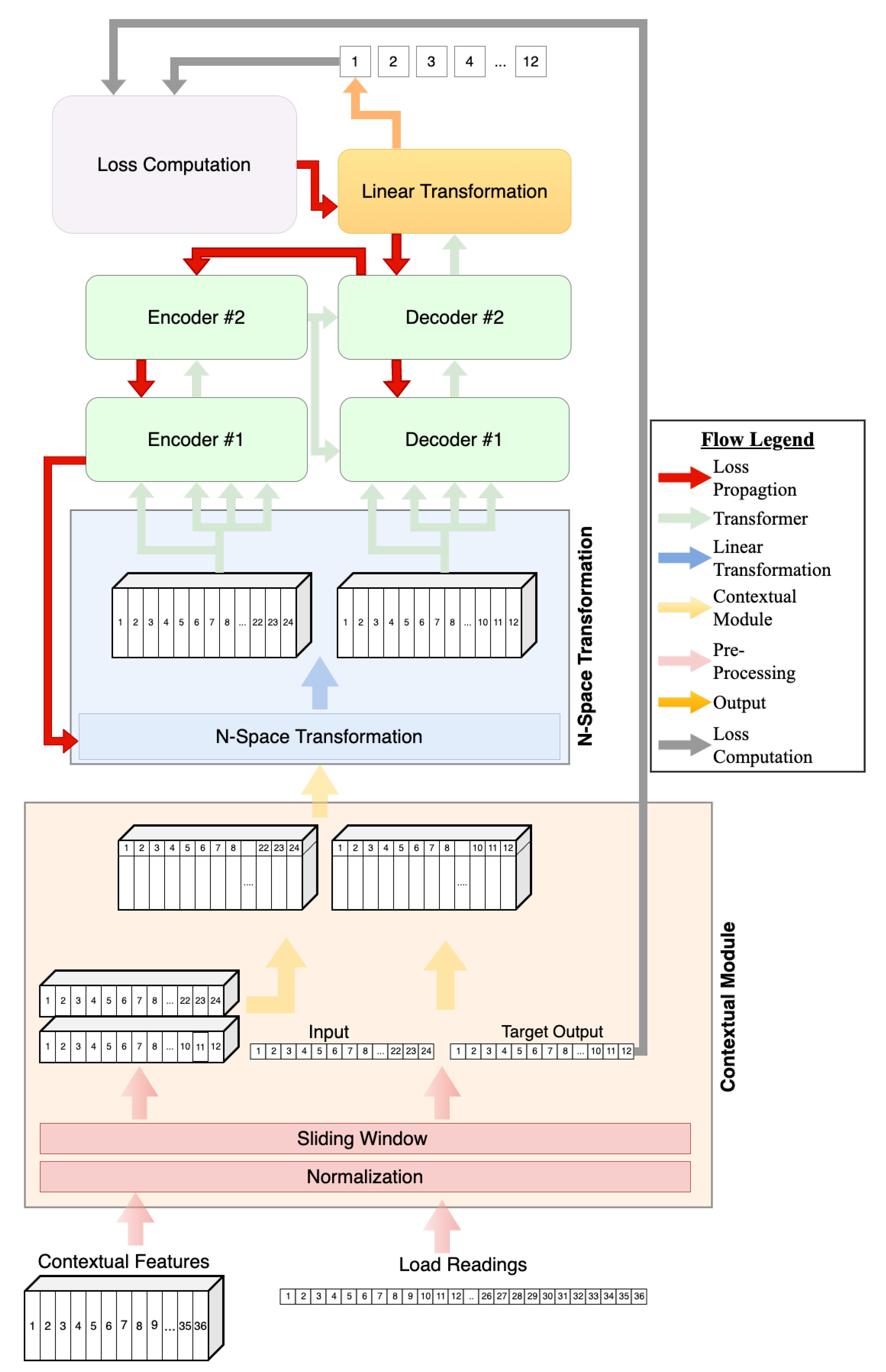
Transformer training is carried out through the contextual model, N-space transformation module, and lastly the actual transformer. Figure 1 depicts the modified architecture.

3.1.1. Contextual Module

The objective of the contextual model is to enable different processing pathways for energy readings and contextual features. Energy readings are both the input to the system and the required output, because past readings are used to predict future consumption. In contrast, contextual features are known values and do not need to be predicted by the transformer. For example, if trying to predict a load 24 steps ahead, the day of the week and the hour of the day for which we are forecasting are known. Therefore, these two components of the data can be processed differently.

The input of the system consists of energy readings combined with contextual features, while the expected output is comprised only of load values. Contextual features commonly used with load forecasting [13] include those extracted directly from the reading date/time, such as time of day and day of the week. After extraction, these features are represented numerically and combined to form contextual vectors.

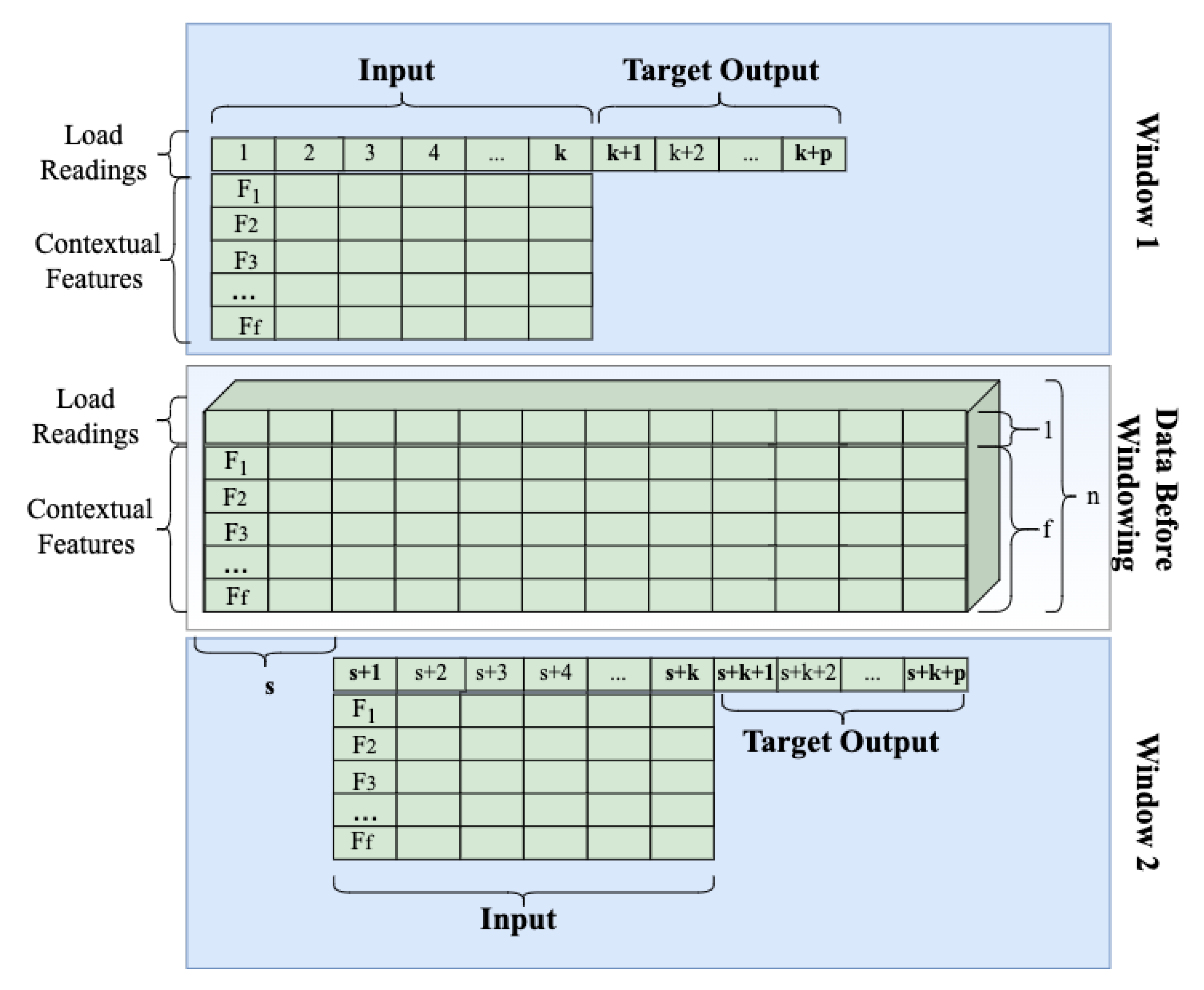
These numerical vectors are merged with load readings, resulting in n features for each time step, where n is the number of contextual features plus one to account for the load reading. At this point, the data are a stream of readings, while the transformer in NLP expects sentences. To convert these streams into a format suitable for transformers, the sliding window technique is used. The process is depicted in detail in Figure 2.

In the sliding window approach, as shown in Figure 2, the first input sample (Window 1) consists of the first k readings, thus one sample has a dimension of $k\times n$ where n is the number of features. If predicting p steps ahead, the expected output contains load readings without contextual features at time steps $k+1$ to $k+p$. Then, the window slides for s steps, the next input sample consists of readings from $s+1$ to $s+k$, and the expected output contains load readings for time steps $s+k+1$ to $s+k+p$. In this study, overlapping sliding widows are used, thus $s<k$.

In training, contextual features with the load values are the inputs to the encoder, while the inputs to the decoder are contextual features with the expected (target) load values. The output of the decoder consists of the predicted load values, which are used to compute the loss function and, consequently, to calculate gradients and update the weights.

3.1.2. N-Space Transformation Module

The purpose of the N-space transformation module is to improve the performance of the multi-headed attention (MHA) component of the transformer by transforming the input data to better capture relationships between energy readings and contextual features. Once the data pass through the contextual module, the energy reading and its contextual features form a vector. That vector $n_t$ at time t is a concatenation of contextual vector $c_t$ and energy reading $e{r}_t$ such that $n_t=(e{r}_t,c_{1t},c_{2t},c_{3t},\dots ,c_{ft})$, where f is the number of contextual features. Therefore, the length of any vector n is equal to the length of $f+1$. In order to enter the encoder, each of the k vectors corresponding to k time steps of the window are stacked together to form an augmented input matrix of dimensions $n\times k$, effectively rotating the matrix.

Since the contextual features are concatenated to the energy reading, only one column of the input matrix contains the energy reading. As multi-head attention (MHA) deals with subsets of features, several heads will only be handling contextual features; however, in energy forecasting, we are interested in the relationship of contextual features with the target variable: energy consumption.

MHA performs attention calculations on different projections of the data as follows:

$$MultiHead(Q,K,V)=Concat(hea{d}_1,\dots ,hea{d}_h)W^o$$

(1)

$$hea{d}_i=Attention(Q{W}_i^Q,K{W}_i^K,V{W}_i^V)$$

(2)

where Q, K, and V are query, key, and value vectors, respectively, used to calculate the attention and taken from the input matrix, $W^o$ are parameters among heads, and $W_i^Q$, $W_i^K$, and $W_i^V$ are projection parameters for Q, K, and V, respectively [12]. Given that h is the number of heads and $d_{model}$ represents the number of input features, the dimensions of the projection parameters are as follows:

$$W_i^Q\in {\mathbb{R}}^{d_{model}\times d_k},W_i^K\in {\mathbb{R}}^{d_{model}\times d_k},W_i^V\in {\mathbb{R}}^{d_{model}\times d_v}{W}^O\in {\mathbb{R}}^{h{d}_v\times d_{model}}$$

(3)

$$d_k=d_v=d_{model}/h=n/h.$$

(4)

The subspace defined by the projection parameters divides the input matrix along the feature dimension n, making each head responsible for only a subset of features, which leads to the energy reading $er$ not being assigned to all heads. Therefore, some heads deal with determining relationships along contextual features only, which is undesirable, as the model is trying to predict energy consumption from other features.

In order to address this challenge while taking full advantage of MHA, the proposed approach transforms the input matrix into a higher N-space before entering the transformer component. Each dimension of the new space becomes a different combination of the original features through the use of a linear transformation such that:

$$\begin{array}{cc}\hfill & I=X·A\hfill \end{array}$$

(5)

$$\begin{array}{cc}\hfill & I=\left[\begin{array}{cccc}e{r}_{11}& c_{11}& \dots & c_{1f}\\ \dots \\ e{r}_{k1}& c_{k1}& \dots & c_{kf}\end{array}\right]·\left[\begin{array}{ccc}{A}_{11}& \dots & A_{1\theta }\\ \dots \\ A_{n1}& \dots & A_{n\theta }\end{array}\right]\hfill \end{array}$$

(6)

$$\begin{array}{cc}\hfill & I=\left[\begin{array}{ccc}(e{r}_{11}{A}_{11}+\dots +c_{1f}{A}_{n1})& \dots & (e{r}_{11}{A}_{1\theta }+\dots +c_{1f}{A}_{n\theta })\\ \dots \\ (e{r}_{k1}{A}_{11}+\dots +c_{kf}{A}_{n1})& \dots & (e{r}_{k1}{A}_{1\theta }+\dots +c_{kf}{A}_{n\theta })\end{array}\right]\hfill \end{array}$$

(7)

where X is the input matrix of dimension $k\times n$, I is the matrix after transformation, and A are the transformation weights which will be learned during training. The size of the transformed space is determined by $\theta$: matrix I has dimension $k\times \theta$ after transformation. The size of $\theta$ becomes a hyperparameter of the algorithm, where finding the appropriate value may require some experimentation; this parameter will be referred to as the model dimension parameter.

After transformation, each component in matrix I includes energy readings, as seen in Equation (7). By distributing the energy reading over many dimensions, we ensure that attention deals with the feature the model is trying to predict.

3.1.3. Transformer Module

The transformer is composed of an encoder and a decoder module, as seen in Figure 1. This study used a stack of two encoders, each one with two attention heads, and the feed-forward neural network following the attention mechanism: this internal encoder architecture is the same as in the original transformer [12]. Matrix I created during N-space transformation is the input to the transformer and the expected output are the energy readings for the desired output window.

The encoder processes input matrix I, and the encoder output gets passed to the two consecutive decoders. Additionally, the decoder receives the expected output window that went through the contextual model and N-space transformation. As in the original transformer, the decoders consist of the attention mechanisms followed by the feed-forward neural network.

After the data travel through the encoder and the decoder, linear transformation is the last step. Transformation produces the predicted energy consumption by receiving data with $\theta$ dimensions and transforming them into a single value, effectively reversing the N-space transformation. The output gets compared to the target output to compute the loss. This loss is then used to compute the gradients and for backpropagation to update weights in the decoder, encoder, and N-space transformation; this process is depicted by the red arrows in Figure 1.

In the original architecture [12], because the decoder receives the expected target value as an input, the input to the decoder is shifted to the right during training to avoid the decoder learning to predict itself as opposed to the next reading. However, in this adaptation, because of the N-space transformation, the input value is no longer the same as the target output, and this step is no longer needed and is handled by various added transformations. However, the decoder input is still processed using a look-ahead mask, meaning that any data from future time steps are hidden until the prediction is made.

Note that the input contains energy consumption for past time steps, while the target output (expected output) is also energy consumption, but for the desired steps ahead. The length of the input specifies how many historical readings the model uses for forecasting, while the length of the output window corresponds to the forecasting horizon. For example, in one of our experiments, we use 24 past readings to predict 12, 24, and 36 time steps ahead.

3.2. Load Forecasting with Trained Transformer

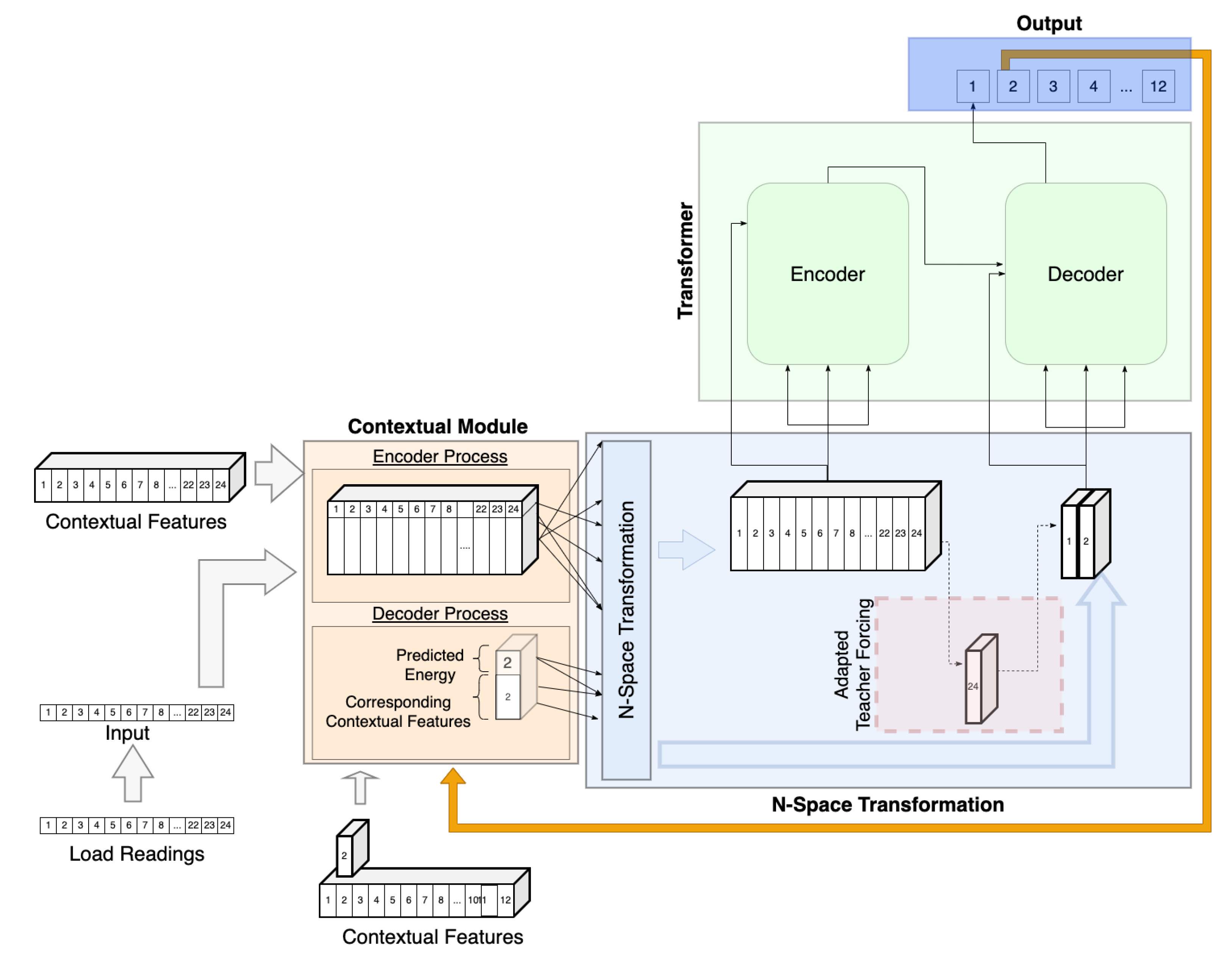
Once again, due to differences in the nature of the input data, further modifications to transformer workflow are required in order to use the trained model for inference tasks. The transformer is composed of an encoder and a decoder module, as seen in Figure 3, which depicts the inference workflow.

3.2.1. Contextual Module

During training, the contextual module is used in the same manner for both the encoder and the decoder because throughout the entire training process data are fully accessible, meaning that actual and expected values can be accessed at any time. However, this is not the case for the inference task because we do not have access to future data.

This difference is particularly significant when dealing with transformers because the transformer builds its output one step at a time and uses each step of the forecasting horizon to predict the next. The input of the decoder at each step consists of all of the previously predicted steps. This is problematic in our workflow because, while the expected input consists of load readings along with their contextual component, the output of the transformer consists only of load readings. Therefore, if we feed the transformer output directly into the decoder, the contextual features will be missing. The goal of the contextual module is to address this shortcoming through separating the contextual and load data pathways.

The typical transformer workflow is modified by sending each output step of the transformer back through the contextual and N-space transformation module before they enter the decoder. The contextual module is responsible for retrieving the corresponding contextual data and creating f features numerical vectors. This is also the case in the training workflow where it has, however, very little impact. At each step t of the prediction, the contextual data are retrieved and transformed into a contextual vector $c_t=(c_{1t},c_{2t},c_{3t},\dots ,c_{ft})$, where f is the number of contextual features. By definition, contextual values such as day, time, and even temperature are either known or external to the system.

After the context is retrieved, the predicted energy reading $pe{r}_t$ is combined with the contextual vector to create a vector n such that $m=(pe{r}_t,c_{1t},c_{2t},c_{3t},\dots ,c_{ft})$. This vector will then go through the N-space transformation module.

3.2.2. N-Space Transformation Module

The N-space transformation module behaves in the same way during inference as it does during training. The only difference is that it is used after each step t of the output as opposed to once.

After each prediction t, the output vector m, which has a dimension equal to $f+1$, is transformed by computing the dot product of vector m to the transformation weights A such that

$$\begin{array}{cc}\hfill & I_t=m·A\hfill \end{array}$$

(8)

$$\begin{array}{cc}\hfill & I_t=\left[\begin{array}{cccc}pe{r}_{t1}& c_{t1}& \dots & c_{tf}\end{array}\right]·\left[\begin{array}{ccc}{A}_{11}& \dots & A_{1\theta }\\ \dots \\ A_{n1}& \dots & A_{n\theta }\end{array}\right]\hfill \end{array}$$

(9)

$$\begin{array}{cc}\hfill & I_t=\left[\begin{array}{ccc}(pe{r}_{t1}{A}_{11}+\dots +c_{tf}{A}_{n1})& \dots & (pe{r}_{t1}{A}_{1\theta }+\dots +c_{tf}{A}_{n\theta })\end{array}\right]\hfill \end{array}$$

(10)

As opposed to during training, where the output matrix I is computed once per input sequence, it is now built slowly over time. Before each next prediction, the newly created vector $I_t$ is combined with those previously created within this forecasting horizon such that the decoder input I is:

$$\begin{array}{cc}\hfill & I=\left[\begin{array}{ccc}(pe{r}_{t1}{A}_{11}+\dots +c_{tf}{A}_{n1})& \dots & (pe{r}_{t1}{A}_{1\theta }+\dots +c_{tf}{A}_{n\theta })\\ (pe{r}_{(t-1)1}{A}_{11}+\dots +c_{(t-1)f}{A}_{n1})& \dots & (pe{r}_{(t-1)1}{A}_{1\theta }+\dots +c_{(t-1)f}{A}_{n\theta })\\ \dots \\ (pe{r}_{(t-q)1}{A}_{11}+\dots +c_{(t-q)f}{A}_{n1})& \dots & (pe{r}_{(t-q)1}{A}_{1\theta }+\dots +c_{(t-q)f}{A}_{n\theta })\end{array}\right]\hfill \end{array}$$

(11)

where q is the number of steps previously predicted and $t<horizon$. This input I is then fed to the decoder.

3.2.3. Transformer Module

The transformer is composed of an encoder and a decoder module, as seen in Figure 3. The encoder’s input is matrix I created by taking a window of historical readings of length k and processing it through the contextual and N-space transformation module in the same manner described in the training workflow. The encoder output then gets passed to the decoder.

Additionally, the decoder receives input matrix I described in the previous subsection. However, one further modification is required when the first prediction is made since there is no previous prediction available to feed the decoder. This modification is described as an adaptive teacher forcing method. The teacher forcing [41] method is a technique used in transformers with NLP where the target word is passed as the next input to the decoder. In our case, such a word is not available; therefore, we make use of an adaptive teacher forcing technique where the input for prediction Step 1 is equal to the last value of the encoder input, that is, the last row of the I input matrix. This step allows us to have an effective starting point for our predictions without compromising future results.

4. Evaluation and Results

This section presents the evaluation methodology of our various experiments, along with their results.

4.1. Evaluation Methodology

In order to evaluate the suitability of the proposed architecture for load forecasting, solutions are evaluated by performing load predictions under various settings and comparing those results with the state-of-the-art method.

In the evaluation, we compare the proposed transformer approach with S2S, as S2S has been shown to outperform RNN approaches based on GRUs, LSTMs, and other neural networks, including feedforward neural networks [36]. Note that the original transformer [12] cannot be directly used for comparison as it is designed for text and is not directly applicable to load forecasting. The S2S model with attention [37] achieves very similar accuracy to the S2S model while significantly increasing computational complexity [37]; therefore, the S2S model is used for comparison.

Fekri et al. [11] argue that it is not sufficient to evaluate and compare load forecasting results on one data stream, and that evaluation on a single stream may lead to misleading conclusions. Therefore, in order to validate the portability and repeatability of our results, various data streams are used. Moreover, different input lengths and forecasting horizons must also be considered, as the algorithm may perform better or worse depending on the considered input and output lengths.

Consequently, experiments are conducted to examine the transformer’s and S2S’s behavior for different forecasting horizons and input sequence lengths. Specifically, input lengths of 12, 24, and 36 steps are considered. For each input window length, forecasting horizons of 12, 24, and 36 steps are chosen. This makes 9 experiments for each algorithm, transformer, and S2S; thus, there are 18 experiments per data stream. Our chosen dataset contains 20 different streams, for a total of 360 experiments.

For each data stream, the last 20% of the data was reserved for testing, while the remainder was used for training. Furthermore, to avoid getting stuck in local minima [13], training was repeated 10 times for each experiment and for both algorithms, with the best-performing model being selected.

In order to assess the accuracy of the models, the most commonly used metrics in load forecasting—mean absolute percentage error (MAPE), mean absolute error (MAE), and root mean square error (RMSE) [42]—are used. These metrics can be formally defined as follow:

$$\mathrm{MAPE}=\frac{1}{N}\sum _{t=1}^N\frac{\left|y_t-\widehat{y_t}\right|}{y_t}$$

(12)

$$\mathrm{MAE}=\frac{1}{N}\sum _{t=1}^N\left|y_t-\widehat{y_t}\right|$$

(13)

$$\mathrm{RMSE}=\sqrt{\left(\frac{1}{N}\right){\sum }_{t=1}^N{(y_t-\widehat{y_t})}^2}$$

(14)

where $y_t$ is the actual value, $\widehat{y_t}$ the predicted value, and N the total number of samples. All metrics, MAPE, MAE, and RMSE, are calculated after the normalized values are returned to their original scale.

4.2. Data Set and Pre-Processing

The experiments were conducted on an open-source dataset [43] containing aggregated hourly loads (in kW) for 20 zones from a US utility company. Therefore, 20 different data streams were used. Each of these streams contains hourly data for 487 days or 11,688 consecutive readings. Hourly prediction was selected for experiments over daily predictions as it is a more challenging problem due to random intraday variations: the literature shows that the same approaches achieve better accuracy for daily predictions than for hourly predictions [10]. The dataset provided the usage, hour, year, month, and day of the month for each reading. The following temporal contextual features were also (created from reading date/time): day of the year, day of the week, weekend indicator, weekday indicator, and season. During the training phase, the contextual information and the load value were normalized using standardization [36] with the following equation:

$$\widehat{x}=\frac{x-\mu }{\sigma }$$

(15)

where x is the original vector, $\widehat{x}$ is the normalized value, and $\mu$ and $\sigma$ are the mean and standard deviation of the feature vector, respectively.

Once normalized, the contextual information and data streams were combined using the temporal information, and then a window sliding technique was applied to create appropriate samples. In order to increase our training and testing set, an overlap of the windows was allowed, and step s was set to 1.

4.3. Model Structure and Hyperparameter Tuning

Experiments were conducted on a machine running Ubuntu OS with an AMD Ryzen 4.20 GHz processor, 128 GB DIMM RAM, and four NVIDIA GeForce RTX 2080 Ti 11 GB graphics cards. In order to alleviate processing time, GPU acceleration was used while training the models. The models were developed using the PyTorch library.

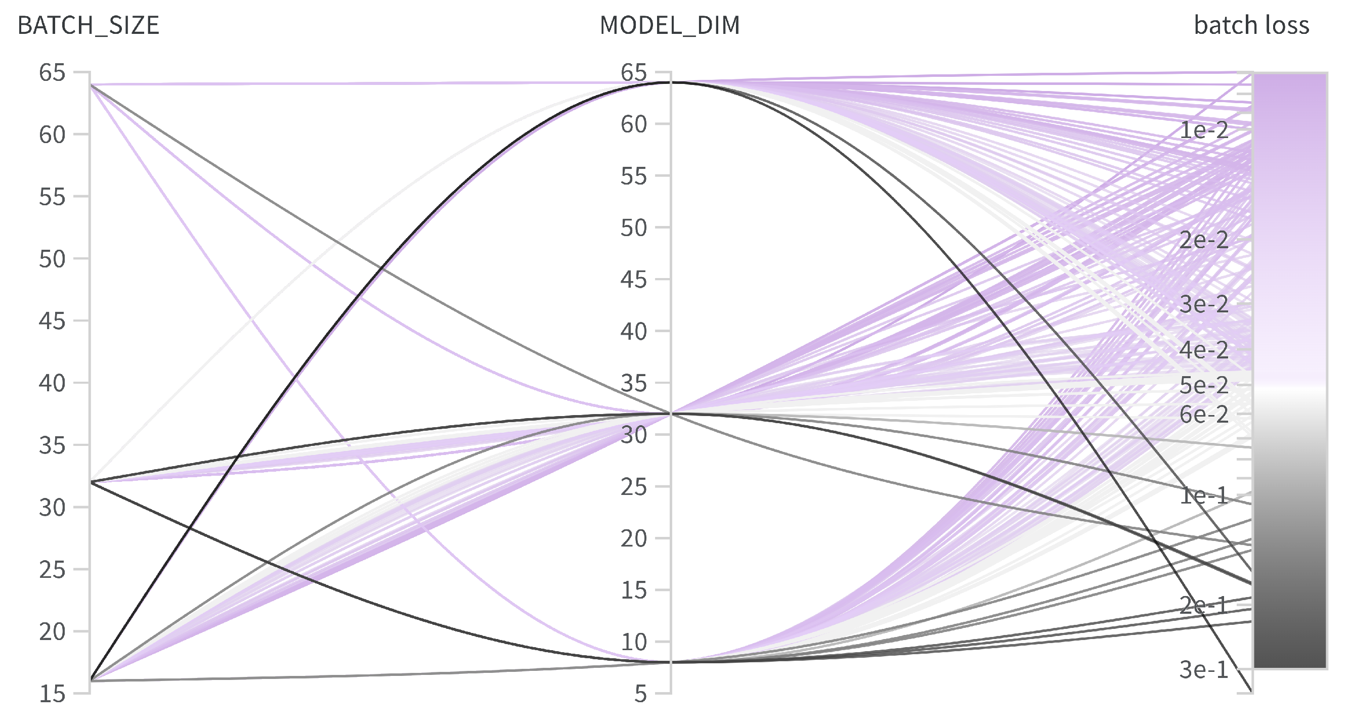
The transformer used in these experiments was made up of a stack of two encoders, two decoders, and two attention heads, and the feed-forward neural network in each encoder and decoder contained 512 neurons. The fully connected hidden layers of the transformer are those of the feed-forward networks embedded in the encoder and decoder; they use ReLU activation function. The Adam optimizer [44] was used during training, with beta values of 0.9 and 0.98 and epsilon values of $1\times {10}^{-9}$ as suggested by Vaswani et al. [12]. The learning rate along with the transformer dropout [45] rate used to prevent overfitting, the N-space dimension, and the batch size used to send data to the transformer were optimized using a Bayesian optimization approach on the Weights and Biases platform [46]. A total of 3477 runs were performed in order to identify the most relevant hyperparameters. Figure 4 shows the importance of each hyperparameter and whether or not it has a positive or negative correlation with optimizing loss.

Based on the information received by the sweeps, we were able to establish that the models appeared to reach convergence after 13 epochs, and that a learning rate of 0.001 and a dropout of 0.3 yielded the best batch loss. However, the optimal N-space dimension (model_dim) and batch size were not as easily determined. A visualization of these parameters shown in Figure 5 allowed us to choose a batch size of 64 and a model dimension of 32 because they appear to best minimize the overall loss. The model dimension refers to size $\theta$ of the N-space transformation module. Lastly, transformer weights were initialized using the Xavier initialization, as it has been shown to be effective [47,48].

The S2S algorithm used for comparison was built using GRU cells, with a learning rate of 0.001, 128 hidden layers, and 10 epochs. These parameters were established as successful in previous works [13,36]. Therefore, the chosen S2S implementation is comparable to the one proposed by Sehovac et al. [36,37].

4.4. Results

This section presents the results obtained in the various experiments and discusses findings.

4.4.1. Overall Performance

The goal of these experiments is to assess the ability of the transformer to predict electrical load under different circumstances. In order to establish the impact of the size of the input window on performance, 12, 24, and 36 historical samples were used as input for each experiment. Note that the size of the input window corresponds to the number of consecutive lagged values, or lag length, used for the prediction. Additionally, since accuracy on one horizon does not guarantee good performance on another [11], forecasting horizons of 12, 24, and 36 steps were also tested. Each of these parameters was evaluated in combination for a total of 9 experiments per stream.

The detailed average statistics over all 20 streams can be seen in

Table 1. Average accuracy over the streams for each combination of input size and forecasting horizon. The bold numbers indicate where transformers outperform S2S.

Input Window	Horizon	MAPE		MAE		RMSE
		Trans.	S2S  [36]	Trans.	S2S  [36]	Trans.	S2S  [36]
12	12	0.0946	0.1039	6180.46	6262.3	8475.7	8350.62
12	24	0.1035	0.1274	6863.35	7812.95	9695.31	10,351.87
12	36	0.1076	0.1397	7045.74	8564.05	9969.6	11,267.95
24	12	0.1077	0.0931	6607.1	5622.66	9043.54	7665.2
24	24	0.1118	0.1148	7011.42	7166.48	9717.14	9659.01
24	36	0.1122	0.1271	7267.98	8166.71	10,347	10,860.76
36	12	0.0888	0.088	5853.8	5465.43	8002.23	7440.19
36	24	0.0928	0.1046	6197.62	6779.88	8649.07	9117.58
36	36	0.0975	0.1276	6794.74	8010.88	9542.88	10,660.9

. It can be observed that 7 out of 9 times, the transformer outperforms S2S [36]. MAPE accuracy differences range from 0.93% to 3.21%, with the transformer performing 1.21% better on average when considering all experiments and 1.78% when considering only the experiments where the transformer outperforms S2S [36].

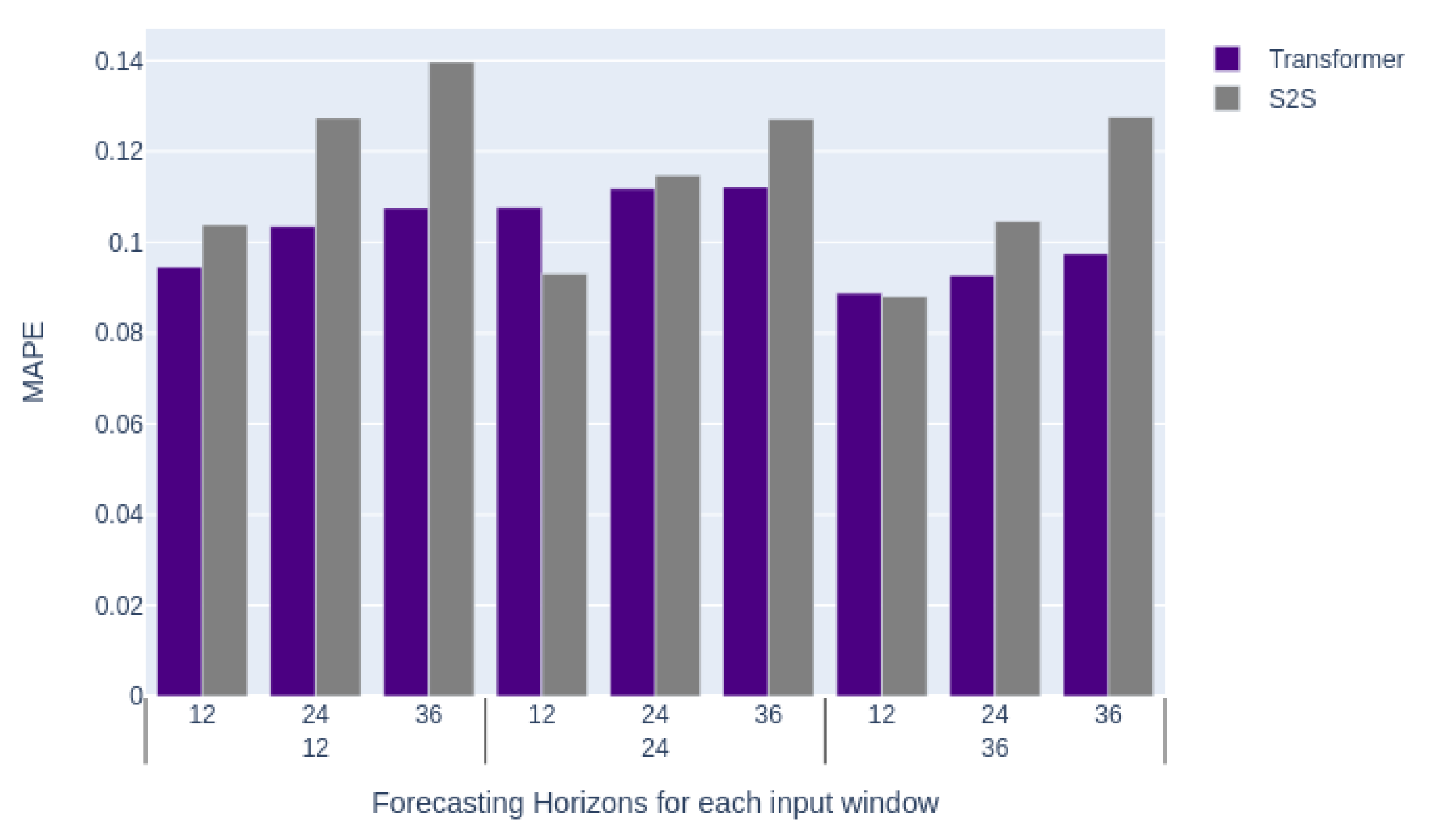
The average of all stream results for each of these experiments is shown in Figure 6. In this case, only MAPE is shown, as MAE and RMSE exhibit similar behavior. In Figure 6, we can make various observations such that the transformer performs much better than S2S [36] when using a 12 h input window, but that the results are much closer when dealing with a 24 h input window. We can also see that regardless of the input size, the transformer outperforms S2S [36] significantly when using a 36 h horizon.

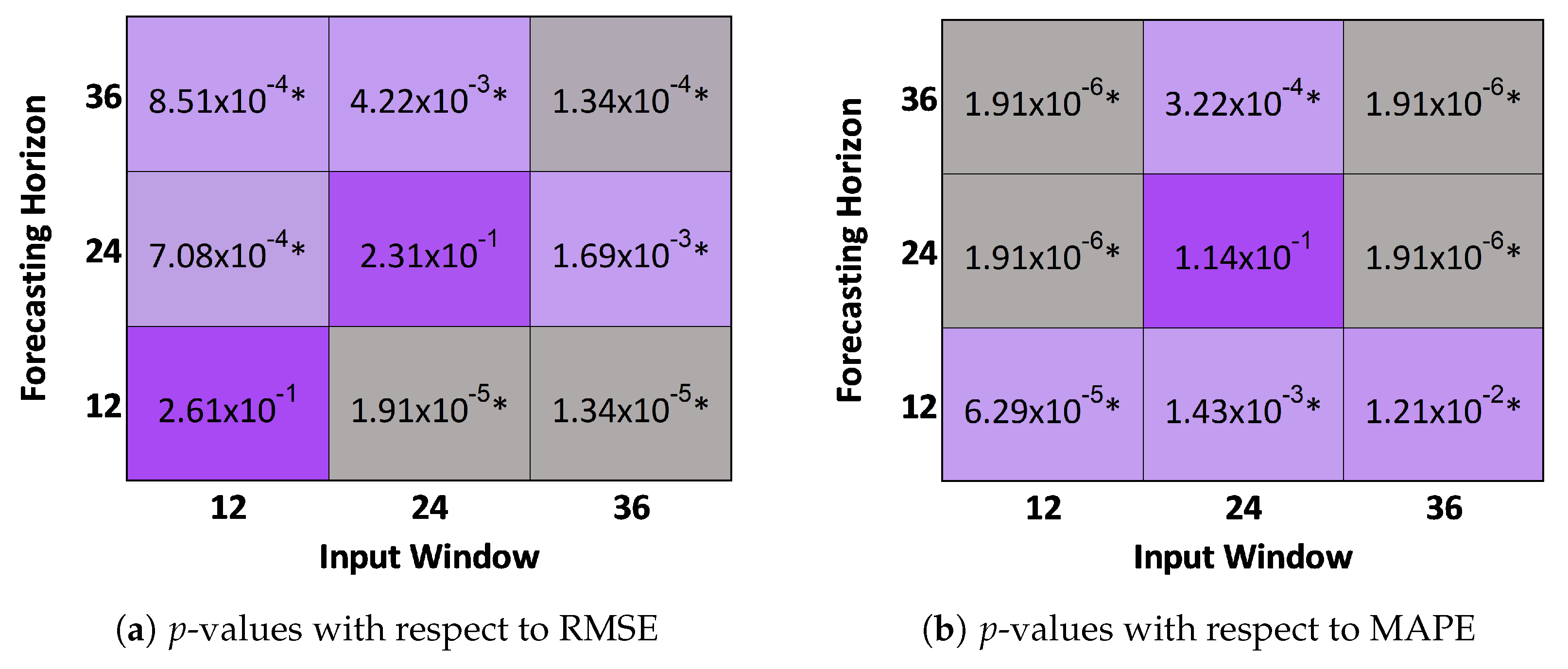
In order to assess the significance of the improvements the proposed transformer model achieves over the state-of-the-art S2S [36], the two-sided Wilcoxon signed-rank test [49] was performed with respect to MAPE and RMSE. This method has been used in the context of energy predictions and electrical load forecasting [50,51,52] and allows us to establish whether the reported model errors are significantly different. For each of the experiments, the errors obtained by the two models, S2S and our transformer model, were assessed for each of the 20 streams. The p-values for different input window sizes and forecasting horizons are shown in Figure 7.

The results show that for a significance level of $\alpha =0.05$, the errors are significantly different for 7 out of 9 experiments with regard to RMSE, and 8 out of 9 experiments for MAPE, as shown in Figure 7. Therefore, considering statistical tests from Figure 7 and the results shown in Table 1, the proposed transformer model achieves overall better accuracy than the S2S model.

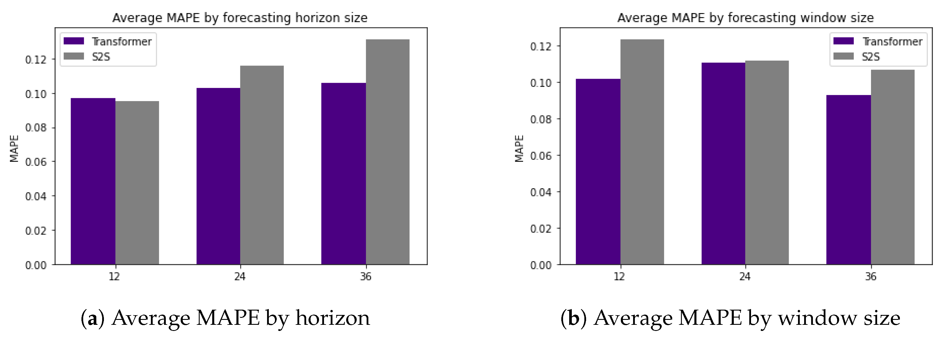
In order to investigate these observations further, we present the average performance for each forecasting horizon over all streams and experiments in

Table 2. Average performance metric per forecasting horizon. The bold numbers indicate where transformers outperform S2S.

Horizon	MAPE		MAE		RMSE
	Trans.	S2S  [36]	Trans.	S2S  [36]	Trans.	S2S  [36]
12	0.0970	0.0950	6213.7865	5783.4636	8507.1582	7818.6714
24	0.1027	0.1156	6690.7948	7253.1038	9353.8385	9709.4885
36	0.1057	0.1315	7036.1531	8247.2149	9953.1587	10,929.8686

. We can observe that the transformer performs better than S2S [36] for longer forecasting horizons, but has similar short-term performance. When predicting 36 steps ahead, the transformer performs 2.571% better on average than S2S [36]. These results are also highlighted in Figure 8a.

Similarly,

Table 3. Average performance metric per input window. The bold numbers indicate where transformers outperform S2S.

Horizon	MAPE		MAE		RMSE
	Trans.	S2S  [36]	Trans.	S2S  [36]	Trans.	S2S  [36]
12	0.1019	0.1237	6696.5146	7546.4348	9380.2027	9990.1481
24	0.1105	0.1116	6962.1674	6985.2825	9702.5603	9394.9921
36	0.0930	0.1067	6282.0524	6752.0650	8731.3925	9072.8884

shows aggregated results over various input window sizes. We can observe that transformers perform better than S2S [36] when provided with smaller amounts of data or shorter input sequences. The transformer outperforms S2S [36] by 2.18% on average using a 12-reading input window. These results are also highlighted in Figure 8b.

Zhao et al. [40] also employed the transformer for load forecasting; however, they used similar days’ load data as the input for the transformer, while our approach uses previous load readings together with contextual features. Consequently, in contrast to the approach proposed by Zhao et al. [40], our approach is flexible with regard to the number of lag readings considered for the forecasting [40], as demonstrated in experiments. Moreover, Zhao et al. handle contextual features outside of the transformer and employ a transformer with six encoders and six decoders, which increases computational complexity.

4.4.2. Stream-Based Performance

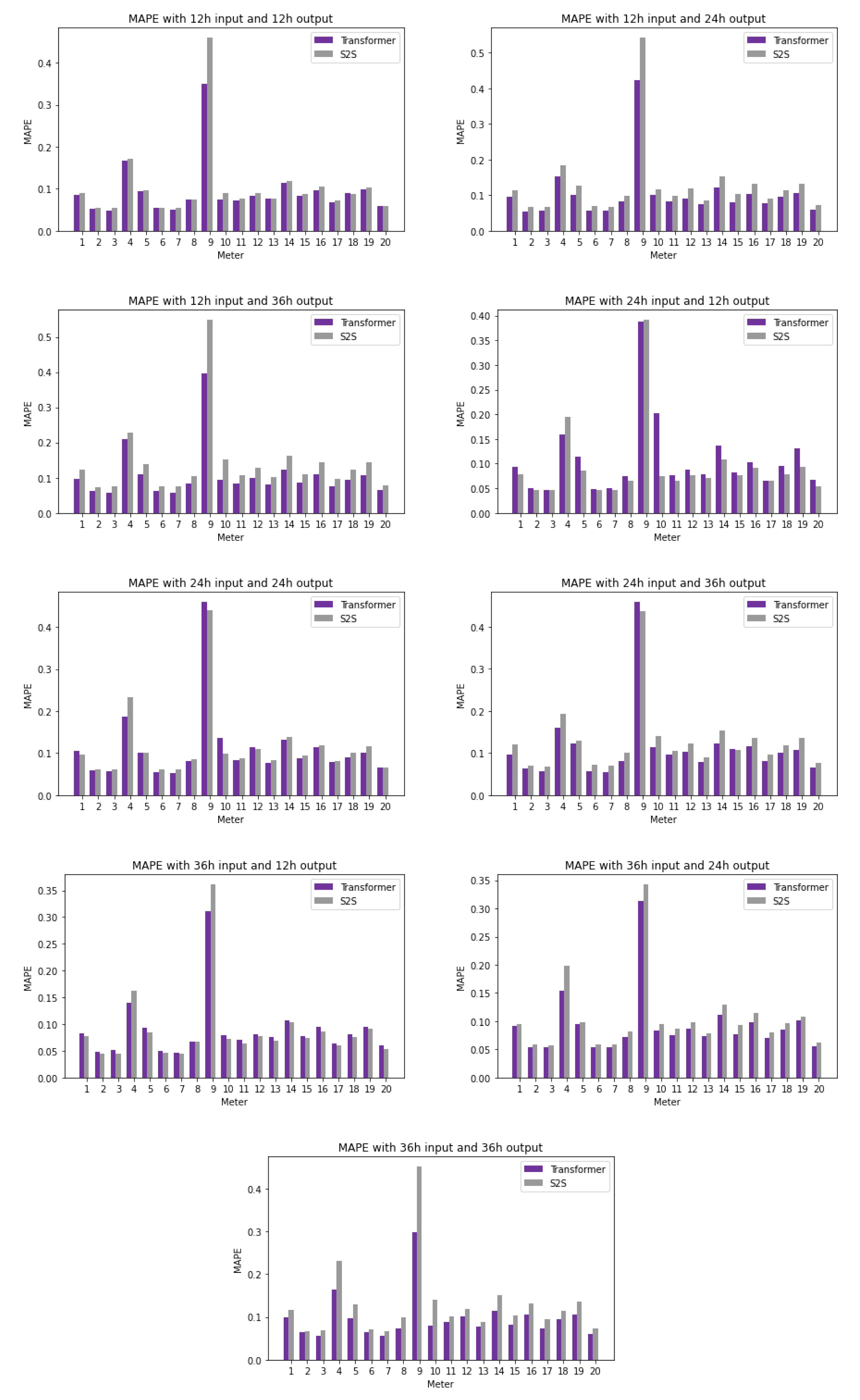
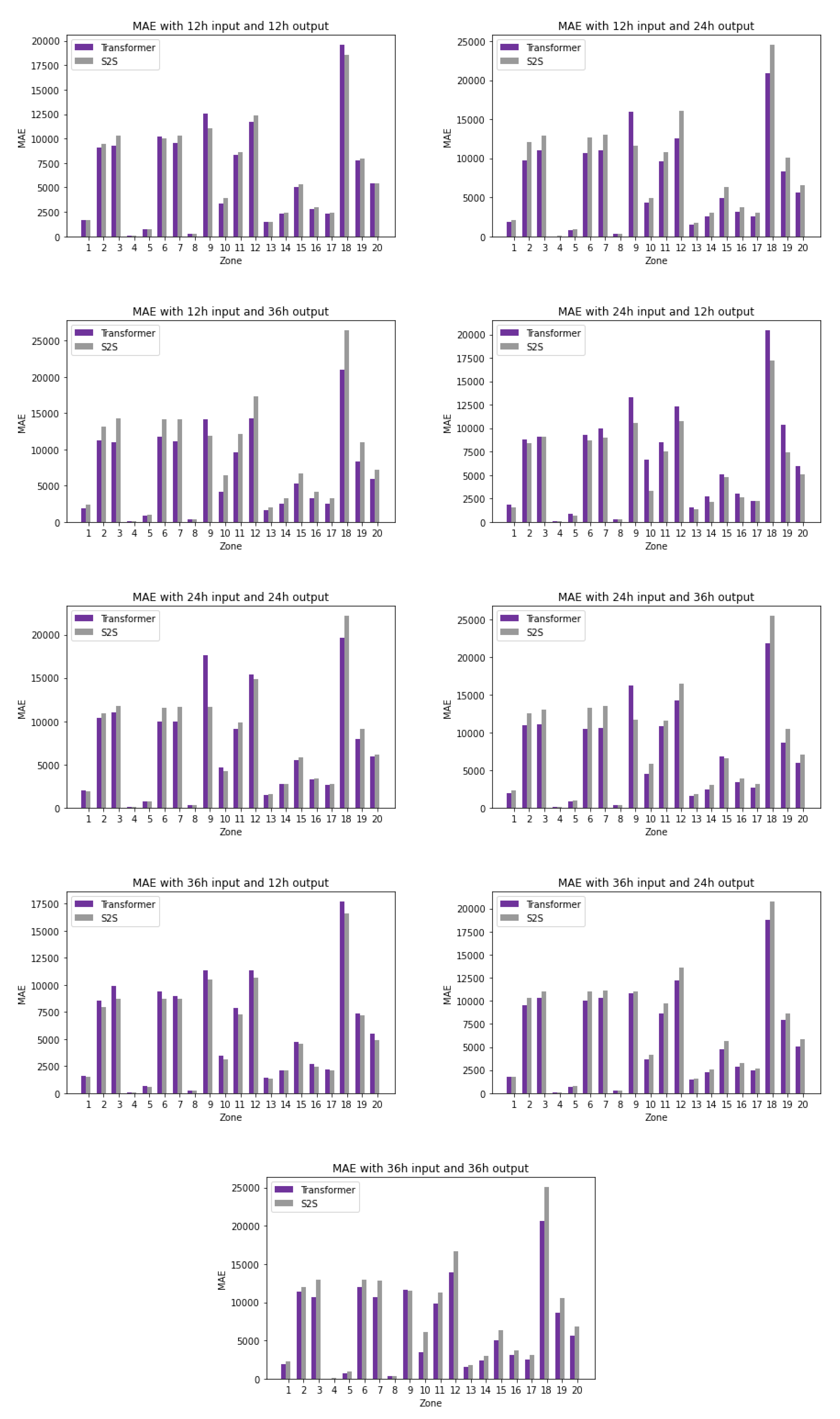
The previous subsection showcased the overall performance of transformers; however, the accuracy of the individual streams must also be investigated. Figure 9, Figure 10 and Figure 11 depict the performance of each stream under each window size and forecasting horizon over the three main metrics: MAPE, MAE, and RMSE. Visualization of the various metrics highlights some differences in results. For example, looking at detailed MAPE results shows that Zones 4 and 9 appear to behave differently than others. The MAE and RMSE show large variance in the ranges of data that we would not have otherwise observed.

After looking at the detailed results of each experiment, we further investigated the average accuracy of each stream. The results are shown in

Table 4. Accuracy comparison of S2S and Transformer for each Stream. The bold numbers indicate where transformers outperform S2S.

Zone	MAPE		MAE		RMSE
	Trans.	S2S  [36]	Trans.	S2S  [36]	Trans.	S2S  [36]
1	0.0939	0.1012	1826.3836	1929.7862	2540.3900	2607.0799
2	0.0561	0.0606	9955.8756	10,766.6417	13,568.4506	14,284.679
3	0.0539	0.0603	10,379.6343	11,554.4385	14,299.3237	15,336.5755
4	0.1660	0.1992	36.4677	36.0893	52.0658	49.6033881
5	0.1031	0.1100	761.4848	802.5733	1052.5361	1078.32458
6	0.0560	0.0619	10,434.4980	11,459.4040	14,215.9081	15,204.1639
7	0.0531	0.0606	10,246.9099	11,588.6249	14,084.0466	15,359.2081
8	0.0766	0.0863	298.2776	337.0904	412.7754	446.240376
9	0.3780	0.4420	13,743.3821	11,256.9949	21,161.6973	15,840.7173
10	0.1069	0.1085	4238.9889	4663.3933	6007.8092	6628.53789
11	0.0805	0.0883	9140.0013	9842.5011	12,841.2556	13,162.449
12	0.0939	0.1046	13,109.0104	14312.1861	18,581.9497	19,152.9508
13	0.0769	0.0827	1486.8373	1614.8049	1996.4151	2126.63412
14	0.1200	0.1352	2445.5682	2696.8011	3335.8576	3543.05389
15	0.0846	0.0945	5235.9749	5785.0526	6953.8205	7544.27375
16	0.1050	0.1176	3058.6245	3351.4500	4283.1468	4471.78485
17	0.0723	0.0820	2457.7264	2759.0086	3346.5709	3644.62272
18	0.0919	0.1012	20,060.7726	21,882.9082	27,734.4832	29,208.1563
19	0.1058	0.1176	8363.9343	9147.0767	11,380.2885	12,026.7175
20	0.0620	0.0661	5657.8772	6105.0565	7578.9121	8004.41788

. The average MAPE accuracy of each stream over all window sizes and horizons is 10.18% for transformers and 11.40% for S2S [36], but it can be seen in Table 4 that it varies from 5.31% to 37.8%. The transformer’s MAPE for the majority of the zones is below 12%. The exceptions are Zones 4 and 9, which have higher errors; still, the transformer outperforms S2S [36].

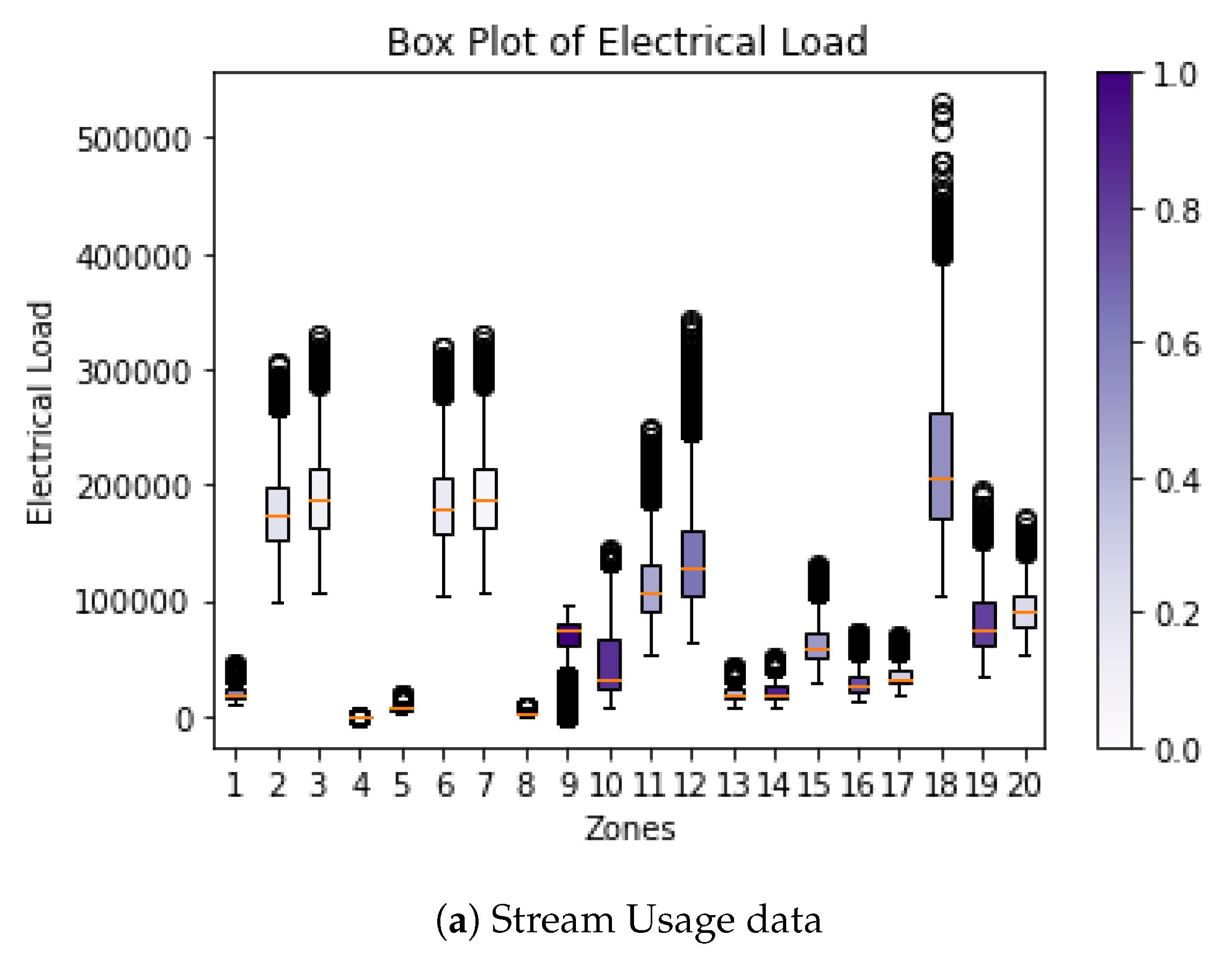
Based on the observed detailed results for each experiment presented in Figure 9, Figure 10 and Figure 11, we further investigate the variability of data. For each stream, variance was drawn using both normalized and un-normalized data. The results are shown in Figure 12.

It can be observed that the two streams that appeared to perform differently, 4 and 9, have a high number of outliers close to 0, which can affect accuracy. This may explain why, regardless of the algorithm used, the error is higher than with other streams.

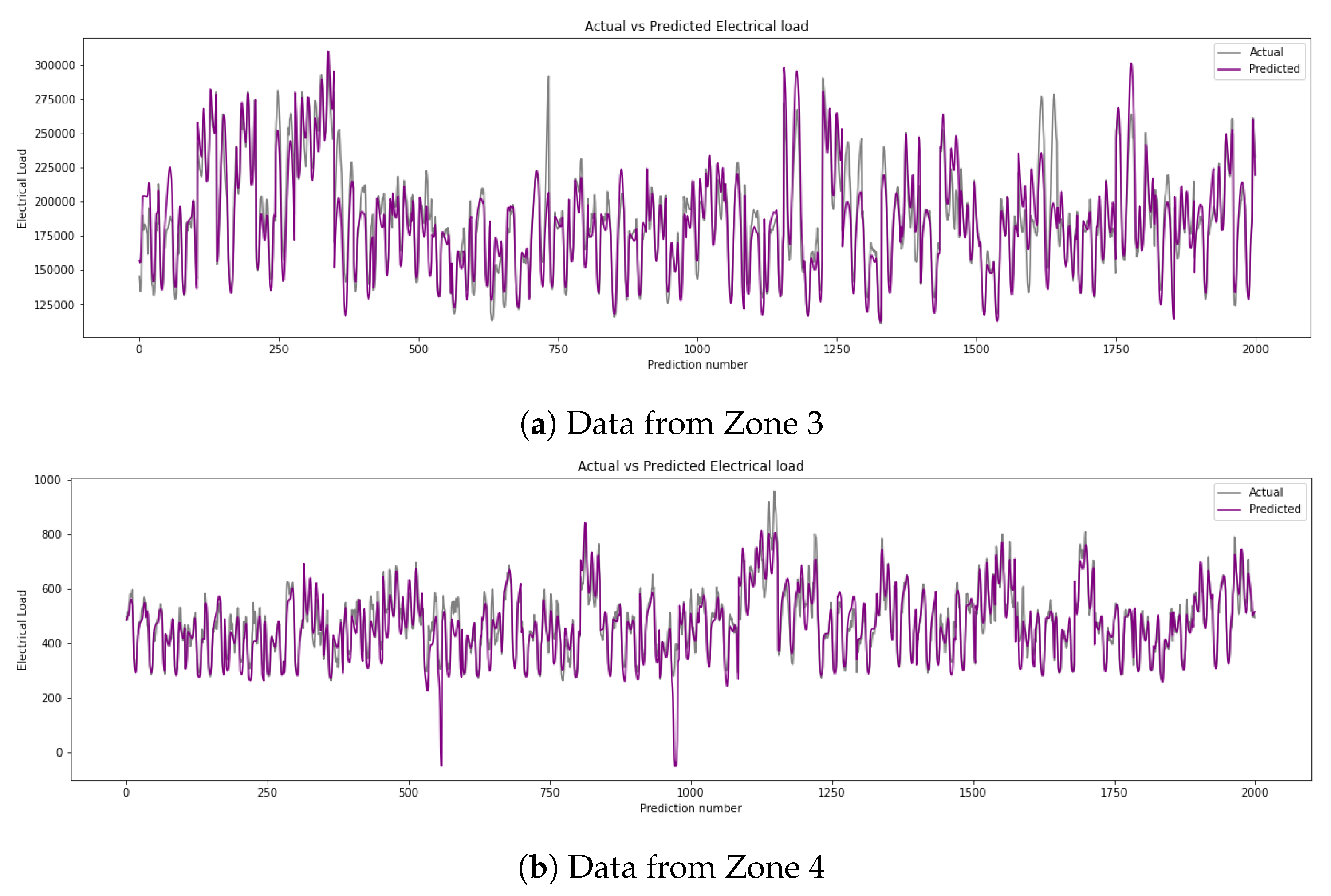
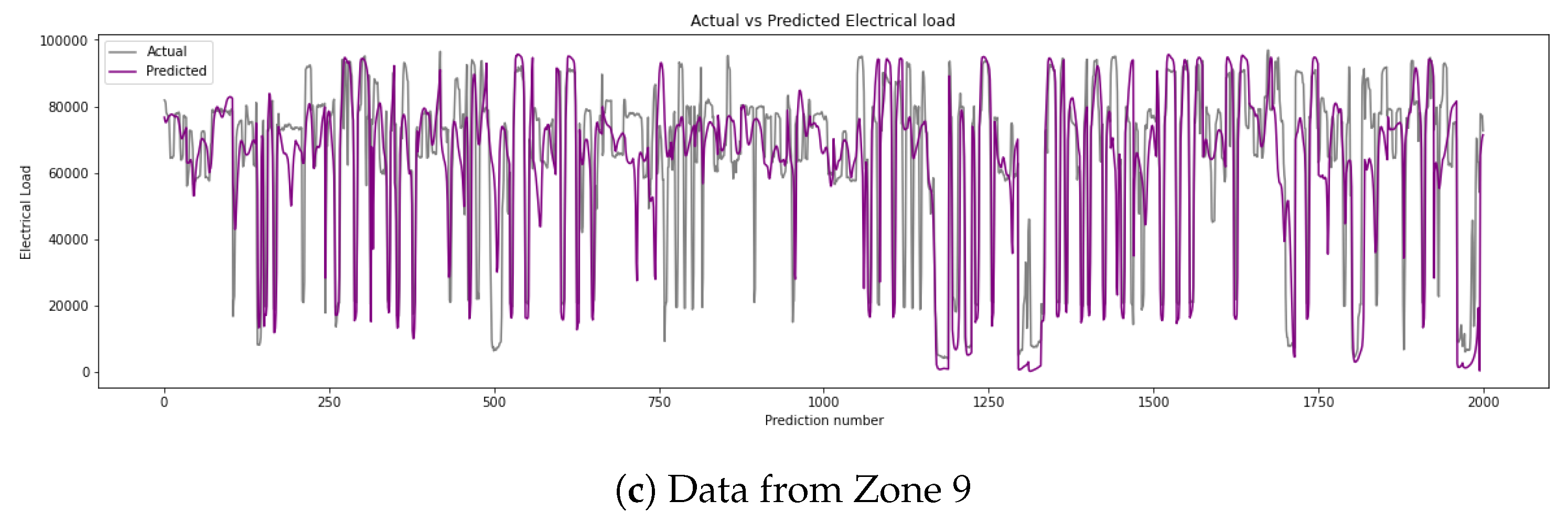
To visually illustrate the accuracy of the prediction results, the predicted and actual energy readings using a 36-step input and 36-step horizon for the streams for Zones 3, 4, and 9 are shown in Figure 13. The models shown have MAPEs of 0.05484, 0.1636, and 0.2975, respectively. The models appear to capture the variations quite well; however, lower values do appear to create some inconsistencies in prediction. These graphs only show a subset of the predicted test set but are able to showcase the differences across the various streams, such as differences in range, minimum and maximum values, and overall patterns of consumption.

In order to gain insight into the ability of the transformer to perform accurately over various streams using different input sizes,

Table 5. Comparison of average MAPE for each stream over each input size. The bold numbers indicate where transformers outperform S2S.

Zone	36		24		12
	Trans.	S2S  [36]	Trans.	S2S  [36]	Trans.	S2S  [36]
1	0.0907368	0.09602993	0.09875669	0.09860627	0.09222631	0.10894584
2	0.05524482	0.05683472	0.05724595	0.05962232	0.05577322	0.06546532
3	0.05346749	0.05671243	0.05385202	0.05880784	0.05433251	0.06546107
4	0.15230604	0.19670615	0.1685036	0.20666588	0.17727173	0.19410134
5	0.09420072	0.10373397	0.1129271	0.1058648	0.10224154	0.12029345
6	0.05647846	0.05869588	0.053517	0.05992111	0.05798402	0.06702744
7	0.05167302	0.05682455	0.05256521	0.05955054	0.0549446	0.06536387
8	0.07150024	0.0822365	0.07872773	0.08415244	0.07949735	0.0925331
9	0.3074255	0.38559468	0.43601709	0.42283669	0.39044071	0.51743441
10	0.08068328	0.10279355	0.15054447	0.10421485	0.08943305	0.11862457
11	0.07755393	0.08442687	0.0849148	0.08620438	0.07908267	0.09419119
12	0.08964494	0.0983836	0.10155942	0.10269988	0.09059058	0.11256996
13	0.07574321	0.07863231	0.07783259	0.08117275	0.07722563	0.08839613
14	0.11062324	0.12798273	0.12961384	0.13304362	0.11961636	0.14470344
15	0.07822967	0.09031995	0.0929283	0.0928472	0.0825027	0.1003986
16	0.09933909	0.11099539	0.1115117	0.11485636	0.10415954	0.12690634
17	0.06939691	0.07811709	0.07495881	0.08085506	0.07251007	0.08701767
18	0.0867606	0.09528691	0.09568781	0.09993103	0.09310351	0.10825483
19	0.10059118	0.11143918	0.11338793	0.11526007	0.10335356	0.12596767
20	0.05852363	0.06298088	0.06571468	0.06576078	0.06162274	0.06956308

shows the average MAPE for each stream over each input size. It can be observed that transformers outperform S2S [36] 55 times out of 60. Therefore, we can conclude that transformers can outperform S2S [36] in the majority of cases, regardless of variance within data streams.

5. Conclusions

Transformers have revolutionized the field of natural language processing (NLP) and have rendered NLP tasks more accessible through the development of large pre-trained models. However, such advancements have not yet taken place in the field of load forecasting.

This paper investigated the suitability of transformers for load forecasting tasks and provided a means of adapting existing transformer architecture to perform such tasks. The model was evaluated through comparisons with a state-of-the-art algorithm for energy prediction, S2S [36], and it was shown to outperform the latter under various input and output settings. Furthermore, repeatability of the results was successfully challenged by testing the model on a large number of data streams.

On average, the proposed architecture provided a 2.571% MAPE accuracy increase when predicting 36 h ahead, and an increase of 2.18% when using a 12 h input windo. The solution performed better on longer horizons with smaller amounts of input data. The transformer provided increased accuracy more than 90% of the time while having the potential to be parallelized to further improve performance.

Transformers have been shown to be highly reusable when pre-trained on large amounts of data, making NLP models more easily deployable and accessible for a variety of tasks. Future work will investigate the possibility of creating a pre-trained transformer to perform load forecasting tasks for the masses and investigate performance improvements through transformer parallelization.

References

- Walther, J.; Weigold, M. A systematic review on predicting and forecasting the electrical energy consumption in the manufacturing industry. Energies 2021, 14, 968. [Google Scholar] [CrossRef]
- International Energy Agency. Net Zero by 2050—A Roadmap for the Global Energy Sector; Technical Report; IEA Publications: Paris, France, 2021. [Google Scholar]
- U.S. Energy Information Administration (EIA). Frequently Asked Questions (FAQs). How Much Carbon Dioxide Is Produced Per Kilowatthour of U.S. Electricity Generation. 2021. Available online: https://www.eia.gov/tools/faqs/faq.php?id=74&t=11 (accessed on 20 May 2022).
- Lo Cascio, E.; Girardin, L.; Ma, Z.; Maréchal, F. How Smart is the Grid? arXiv 2020, arXiv:2006.04943. [Google Scholar] [CrossRef]
- Shabanzadeh, M.; Moghaddam, M.P. What is the Smart Grid? Definitions, Perspectives, and Ultimate Goals. In Proceedings of the 28th International Power System Conference, Tehran, Iran, 13 November 2013. [Google Scholar]
- Zheng, J.; Xu, C.; Zhang, Z.; Li, X. Electric load forecasting in smart grids using Long-Short-Term-Memory based Recurrent Neural Network. In Proceedings of the 2017 51st Annual Conference on Information Sciences and Systems, CISS 2017; Institute of Electrical and Electronics Engineers Inc.: New York, NY, USA, 2017. [Google Scholar] [CrossRef]
- Aung, Z.; Toukhy, M.; Williams, J.; Sanchez, A.; Herrero, S. Towards Accurate Electricity Load Forecasting in Smart Grids. In Proceedings of the 4th International Conference on Advances in Databases, Knowledge, and Data Applications, Saint Gilles, France, 29 February–5 March 2012. [Google Scholar]
- Zhang, X.M.; Grolinger, K.; Capretz, M.A.; Seewald, L. Forecasting Residential Energy Consumption: Single Household Perspective. In Proceedings of the 17th IEEE International Conference on Machine Learning and Applications, ICMLA, Orlando, FL, USA, 17–20 December 2018; pp. 110–117. [Google Scholar] [CrossRef]
- Jagait, R.K.; Fekri, M.N.; Grolinger, K.; Mir, S. Load forecasting under concept drift: Online ensemble learning with recurrent neural network and ARIMA. IEEE Access 2021, 9, 98992–99008. [Google Scholar] [CrossRef]
- Grolinger, K.; L’Heureux, A.; Capretz, M.; Seewald, L. Energy Forecasting for Event Venues: Big Data and Prediction Accuracy. Energy Build. 2016, 112, 222–233. [Google Scholar] [CrossRef] [Green Version]
- Fekri, M.N.; Patel, H.; Grolinger, K.; Sharma, V. Deep learning for load forecasting with smart meter data: Online Adaptive Recurrent Neural Network. Appl. Energy 2021, 282, 116177. [Google Scholar] [CrossRef]
- Vaswani, A.; Shazeer, N.; Parmar, N.; Uszkoreit, J.; Jones, L.; Gomez, A.N.; Kaiser, Ł.; Polosukhin, I. Attention is all you need. In Proceedings of the Advances in Neural Information Processing Systems, Long Beach, CA, USA, 4–9 December 2017; Volume 2017. [Google Scholar]
- Tian, Y.; Sehovac, L.; Grolinger, K. Similarity-Based Chained Transfer Learning for Energy Forecasting with Big Data. IEEE Access 2019, 7, 139895–139908. [Google Scholar] [CrossRef]
- L’Heureux, A.; Grolinger, K.; Elyamany, H.F.; Capretz, M.A. Machine Learning with Big Data: Challenges and Approaches. IEEE Access 2017, 5, 7776–7797. [Google Scholar] [CrossRef]
- Li, L.; Ota, K.; Dong, M. When Weather Matters: IoT-Based Electrical Load Forecasting for Smart Grid. IEEE Commun. Mag. 2017, 55, 46–51. [Google Scholar] [CrossRef] [Green Version]
- Hammad, M.A.; Jereb, B.; Rosi, B.; Dragan, D. Methods and Models for Electric Load Forecasting: A Comprehensive Review. Logist. Sustain. Transp. 2020, 11, 51–76. [Google Scholar] [CrossRef] [Green Version]
- Chen, J.F.; Wang, W.M.; Huang, C.M. Analysis of an adaptive time-series autoregressive moving-average (ARMA) model for short-term load forecasting. Electr. Power Syst. Res. 1995, 34, 187–196. [Google Scholar] [CrossRef]
- Huang, S.J.; Shih, K.R. Short-term load forecasting via ARMA model identification including non-Gaussian process considerations. IEEE Trans. Power Syst. 2003, 18, 673–679. [Google Scholar] [CrossRef] [Green Version]
- Pappas, S.S.; Ekonomou, L.; Karampelas, P.; Karamousantas, D.C.; Katsikas, S.K.; Chatzarakis, G.E.; Skafidas, P.D. Electricity demand load forecasting of the Hellenic power system using an ARMA model. Electr. Power Syst. Res. 2010, 80, 256–264. [Google Scholar] [CrossRef]
- Contreras, J.; Espínola, R.; Nogales, F.J.; Conejo, A.J. ARIMA models to predict next-day electricity prices. IEEE Trans. Power Syst. 2003, 18, 1014–1020. [Google Scholar] [CrossRef]
- Nepal, B.; Yamaha, M.; Yokoe, A.; Yamaji, T. Electricity load forecasting using clustering and ARIMA model for energy management in buildings. Jpn. Archit. Rev. 2020, 3, 62–76. [Google Scholar] [CrossRef] [Green Version]
- Scott, G. Box-Jenkins Model Definition. Investopedia—Advanced Technical Analysis Concepts. 2021. Available online: https://www.investopedia.com/terms/b/box-jenkins-model.asp (accessed on 20 May 2022).
- Al-Hamadi, H.M.; Soliman, S.A. Short-term electric load forecasting based on Kalman filtering algorithm with moving window weather and load model. Electr. Power Syst. Res. 2004, 68, 47–59. [Google Scholar] [CrossRef]
- Zhao, H.; Guo, S. An optimized grey model for annual power load forecasting. Energy 2016, 107, 272–286. [Google Scholar] [CrossRef]
- Abd Jalil, N.A.; Ahmad, M.H.; Mohamed, N. Electricity load demand forecasting using exponential smoothing methods. World Appl. Sci. J. 2013, 22, 1540–1543. [Google Scholar] [CrossRef]
- Wang, C.; Chen, M.H.; Schifano, E.; Wu, J.; Yan, J. Statistical methods and computing for big data. Stat. Interface 2016, 9, 399–414. [Google Scholar] [CrossRef] [Green Version]
- de Almeida Costa, C.; Lambert-Torres, G.; Rossi, R.; da Silva, L.E.B.; de Moraes, C.H.V.; Pereira Coutinho, M. Big Data Techniques applied to Load Forecasting. In Proceedings of the 18th International Conference on Intelligent System Applications to Power Systems, ISAP 2015, Porto, Portugal, 18–22 October 2020. [Google Scholar] [CrossRef]
- Cai, M.; Pipattanasomporn, M.; Rahman, S. Day-ahead building-level load forecasts using deep learning vs. traditional time-series techniques. Appl. Energy 2019, 236, 1078–1088. [Google Scholar] [CrossRef]
- Yang, W.; Shi, J.; Li, S.; Song, Z.; Zhang, Z.; Chen, Z. A combined deep learning load forecasting model of single household resident user considering multi-time scale electricity consumption behavior. Appl. Energy 2022, 307, 118197. [Google Scholar] [CrossRef]
- Phyo, P.P.; Jeenanunta, C. Advanced ML-Based Ensemble and Deep Learning Models for Short-Term Load Forecasting: Comparative Analysis Using Feature Engineering. Appl. Sci. 2022, 12, 4882. [Google Scholar] [CrossRef]
- Nilakanta Singh, K.; Robindro Singh, K. A Review on Deep Learning Models for Short-Term Load Forecasting. In Applications of Artificial Intelligence and Machine Learning; Springer: Berlin/Heidelberg, Germany, 2021. [Google Scholar] [CrossRef]
- Xishuang, D.; Lijun, Q.; Lei, H. Short-term load forecasting in smart grid: A combined CNN and K-means clustering approach. In Proceedings of the IEEE International Conference on Big Data and Smart Computing, BigComp, Jeju, Korea, 13–16 February 2017; pp. 119–125. [Google Scholar] [CrossRef]
- Rafi, S.H.; Nahid-Al-Masood; Deeba, S.R.; Hossain, E. A Short-Term Load Forecasting Method Using Integrated CNN and LSTM Network. IEEE Access 2021, 9, 32436–32448. [Google Scholar] [CrossRef]
- Marino, D.L.; Amarasinghe, K.; Manic, M. Building energy load forecasting using Deep Neural Networks. In Proceedings of the IECON 2016—42nd Annual Conference of the IEEE Industrial Electronics Society, Florence, Italy, 23–26 October 2016; pp. 7046–7051. [Google Scholar] [CrossRef] [Green Version]
- Li, D.; Sun, G.; Miao, S.; Gu, Y.; Zhang, Y.; He, S. A short-term electric load forecast method based on improved sequence-to-sequence GRU with adaptive temporal dependence. Int. J. Electr. Power Energy Syst. 2022, 137, 107627. [Google Scholar] [CrossRef]
- Sehovac, L.; Nesen, C.; Grolinger, K. Forecasting building energy consumption with deep learning: A sequence to sequence approach. In Proceedings of the IEEE International Congress on Internet of Things, ICIOT 2019—Part of the 2019 IEEE World Congress on Services, Milan, Italy, 8–13 July 2019; pp. 108–116. [Google Scholar] [CrossRef] [Green Version]
- Sehovac, L.; Grolinger, K. Deep Learning for Load Forecasting: Sequence to Sequence Recurrent Neural Networks with Attention. IEEE Access 2020, 8, 36411–36426. [Google Scholar] [CrossRef]
- Fekri, M.N.; Grolinger, K.; Mir, S. Distributed load forecasting using smart meter data: Federated learning with Recurrent Neural Networks. Int. J. Electr. Power Energy Syst. 2022, 137, 107669. [Google Scholar] [CrossRef]
- Wu, N.; Green, B.; Ben, X.; O’banion, S. Deep Transformer Models for Time Series Forecasting: The Influenza Prevalence Case. arXiv 2020, arXiv:2001.08317. [Google Scholar]
- Zhao, Z.; Xia, C.; Chi, L.; Chang, X.; Li, W.; Yang, T.; Zomaya, A.Y. Short-Term Load Forecasting Based on the Transformer Model. Information 2021, 12, 516. [Google Scholar] [CrossRef]
- Williams, R.J.; Zipser, D. A Learning Algorithm for Continually Running Fully Recurrent Neural Networks. Neural Comput. 1989, 1, 270–280. [Google Scholar] [CrossRef]
- Peng, Y.; Wang, Y.; Lu, X.; Li, H.; Shi, D.; Wang, Z.; Li, J. Short-term Load Forecasting at Different Aggregation Levels with Predictability Analysis. In Proceedings of the IEEE Innovative Smart Grid Technologies-Asia (ISGT Asia), Chengdu, China, 21–24 May 2019. [Google Scholar]
- Kaggle. Global Energy Forecasting Competition 2012—Load Forecasting. Available online: https://www.kaggle.com/c/global-energy-forecasting-competition-2012-load-forecasting/data (accessed on 1 April 2021).
- Kingma, D.P.; Lei Ba, J. Adam: A Method for Stochastic Optimization. arXiv 2014, arXiv:1412.6980. [Google Scholar]
- Srivastava, N.; Hinton, G.; Krizhevsky, A.; Sutskever, I.; Salakhutdinov, R. Dropout: A Simple Way to Prevent Neural Networks from Overfitting. J. Mach. Learn. Res. 2014, 15, 1929–1958. [Google Scholar]
- Biewald, L. Experiment Tracking with Weights and Biases. 2020. Available online: https://www.wandb.com/ (accessed on 1 May 2021).
- Bachlechner, T.; Majumder, B.P.; Mao, H.H.; Cottrell, G.W.; Mcauley, J. ReZero is All You Need: Fast Convergence at Large Depth. arXiv 2020, arXiv:2003.04887. [Google Scholar]
- Huang, X.S.; Pérez, F.; Ba, J.; Volkovs, M. Improving Transformer Optimization Through Better Initialization. In Proceedings of the 37th International Conference on Machine Learning, Virtual, 13–18 July 2020. [Google Scholar]
- Wilcoxon, F. Individual comparisons by ranking methods. Biom. Bull. 1945, 1, 80–83. [Google Scholar] [CrossRef]
- Son, H.; Kim, C.; Kim, C.; Kang, Y. Prediction of government-owned building energy consumption based on an RReliefF and support vector machine model. J. Civ. Eng. Manag. 2015, 21, 748–760. [Google Scholar] [CrossRef]
- Hu, Y.; Qu, B.; Wang, J.; Liang, J.; Wang, Y.; Yu, K.; Li, Y.; Qiao, K. Short-term load forecasting using multimodal evolutionary algorithm and random vector functional link network based ensemble learning. Appl. Energy 2021, 285, 116415. [Google Scholar] [CrossRef]
- Bellahsen, A.; Dagdougui, H. Aggregated short-term load forecasting for heterogeneous buildings using machine learning with peak estimation. Energy Build. 2021, 237, 110742. [Google Scholar] [CrossRef]
Figure 1.
Training workflow.
Figure 2.
Overlapping sliding window with contextual features.
Figure 3.
Load forecasting inference workflow of the transformer architecture.
Figure 4.
Hyperparameter relevance. Green indicates a positive correlation and red a negative correlation.
Figure 5.
Hyperparameter optimization visualization.
Figure 6.
Average MAPE comparison over various input and forecasting horizons between the transformer model and S2S [36].
Figure 7.
Heatmap of the Wilcoxon test p-values. Statistical significance, where p-value < 0.05, is indicated with “*”.
Figure 8.
Comparisons of average MAPE between the transformer model and S2S [36].
Figure 9.
MAPE comparison for each stream under each forecasting horizon and input window size between the transformer model and S2S [36].
Figure 10.
MAE comparison for each stream under each forecasting horizon and input window size between the transformer model and S2S [36].
Figure 11.
RMSE comparison for each stream under each forecasting horizon and input window size between the transformer model and S2S [36].
Figure 12.
Box plot of stream data.
Figure 13.
Usage data of different streams over time.