
Fault Arc Detection Based on Channel Attention Mechanism and Lightweight Residual Network

1
School of Software Engineering, Southeast University, Nanjing 211189, China
2
School of Electrical Engineering, Southeast University, Nanjing 211189, China
3
State Grid Guangdong Electric Power Company, Guangzhou 510600, China
*
Author to whom correspondence should be addressed.
Energies 2023, 16(13), 4954; https://0-doi-org.brum.beds.ac.uk/10.3390/en16134954
Submission received: 4 April 2023
/
Revised: 8 June 2023
/
Accepted: 16 June 2023
/
Published: 26 June 2023
(This article belongs to the Special Issue Advances and Optimization of Electric Energy System)
Abstract
:An arc fault is the leading cause of electrical fire. Aiming at the problems of difficulty in manually extracting features, poor generalization ability of models and low prediction accuracy in traditional arc fault detection algorithms, this paper proposes a fault arc detection method based on the fusion of channel attention mechanism and residual network model. This method is based on the channel attention mechanism to perform global average pooling of information from each channel of the feature map assigned by the residual block while ignoring the local spatial data to enhance the detection and recognition rate of the fault arc. This paper introduces a one-dimensional depth separable convolution (1D-DS) module to reduce the network model parameters and shorten the time of single prediction samples. The experimental results show that the F1 score of the network model for arc fault detection under mixed load conditions is 98.07%, and the parameter amount is reduced by 46.06%. The method proposed in this paper dramatically reduces the parameter quantity, floating-point number and time complexity of the network structure while ensuring a high recognition rate, which improves the real-time response ability to detect arc fault. It has a guiding significance for applying arc fault on the edge side.
1. Introduction
In China, according to the fire statistics released by the National Fire and Rescue Bureau, the number of electrical fires is still high, accounting for more than one-third of the number of various fires. More than 40% of electrical fires are caused by arc faults, which have become the main reason for electrical fire accidents in low-voltage distribution systems [1,2]. In the actual low-voltage distribution network, the arc fault is the most difficult to detect and is highly hazardous [3], so the series arc fault is one of the main culprits of an electrical fire. Therefore, it is of great significance to study the series arc fault detection technology in low-voltage systems to improve the safety of electricity and reduce the damage to peoples’ lives and property [4].
The traditional arc detection method for low-voltage series faults is based on the existence of distortion and high-frequency harmonic components in the current and voltage waveforms of the arc branch [5]. Multi-feature detection is generally based on arc time domain, frequency domain and time–frequency domain. Based on the subtraction of adjacent periodic waveforms, reference [6] used wavelet threshold denoising to extract the feature quantity of fault arc and realize the detection of fault arc. Reference [7] proposed to construct the arc image matrix by fractional Fourier transform of the current signal and used the local binary pattern to describe the characteristics of the matrix graph to detect the arc fault. In reference [8], the flat shoulder value, mutation point, current change rate and subharmonic component in the time domain are extracted and then input into the decision model defined by the author to identify the fault arc.
However, the traditional methods are faced with the problems of threshold setting difficulty, large computational complexity and poor generalization ability while using fast Fourier transform (FFT), discrete wavelet transform (WDT) and other more perfect algorithms for fast calculation. Especially with the increasing proportion of non-linear loads in low-voltage distribution systems [9], the normal current under certain operating conditions is likely to be very close to the time domain and frequency domain of the fault arc, which easily makes the arc detection wrong and missed. Michal et al. [10,11] proposed an algorithm for the incremental decomposition of a signal over time, which is about seven times faster than the FFT and cheaper to implement than FFT in arc fault detection equipment.
With the development of 5G communication technology and artificial intelligence, deep learning algorithms propose new ideas for the research of the above problems. A neural network detection model of an arc fault, which is connected with a cloud computing platform through 5G communication technology and based on current signal input, has attracted the attention of scholars at home and abroad. This kind of neural network model can automatically establish the boundary conditions of arc fault identification by training, without setting the threshold of arc fault detection [12], and has a high accuracy of arc fault identification. Yu et al. [13] proposed an improved AlexNet convolutional network and trained it based on the current data when a series fault arc occurs and obtained good detection results. Wang Y et al. [14] proposed that the ArcNet network can achieve high detection accuracy at a 10 Khz sampling rate and pass the evaluation test of the actual hardware platform.
In this paper, a one-dimensional depth separable residual network model (Faster MA-ResNet) based on the channel attention mechanism, which uses the current data set of arc fault in low-voltage series, is proposed. Firstly, the channel attention mechanism convolution module is embedded in the residual network structure. The neural network can select the channel that is more critical to identify the arc fault across the channel, thereby increasing the prediction accuracy and generalization performance of the neural network. At the same time, considering the problem of network application in the edge scene, this paper introduces a one-dimensional depth separable convolution module, the aim of which is to reduce the number of parameters of the network structure, the number of floating points and the average time of single sample prediction. Under the premise of losing small accuracy, the network structure achieves the purpose of compressing the model and improving the response speed of arc fault detection. At the same time, considering the problems of high cost and poor real-time caused by connecting fault arc detection with a cloud computing platform by using 5G communication technology, this paper introduces a one-dimensional depth separable convolution module, which aims to reduce the parameters of the network structure, floating point numbers and the average time of single sample prediction, so that the network structure can compress the model and improve the response speed of fault arc detection on the premise of losing less accuracy, so as to achieve end-side application.
2. Materials and Methods
2.1. One-Dimensional Channel Attention Mechanism
The attention mechanism in deep learning is generated by the observation mechanism of human beings on the outside, which implies a tendency to focus on local information of higher importance among a large amount of information and to select the information that is more critical for the learning of the current objects, intending to obtain the overall cognition of the current objects [15]. The attention mechanism is divided into the soft-attention mechanism and the hard-attention mechanism [16]. The soft attention mechanism is a way of paying attention to the overall situation. The weight assigned to each input item is between 0 and 1, which means different weight ratios are assigned to the input item.
The soft attention mechanism pays more attention to the channel or space. The channel attention mechanism obtains the weight of each feature channel through autonomous learning to form a weight matrix on the dimension of the channel. In the weight matrix, the greater weight indicates that the corresponding channel is more important for global learning, and the feature information of the channel is more relevant.
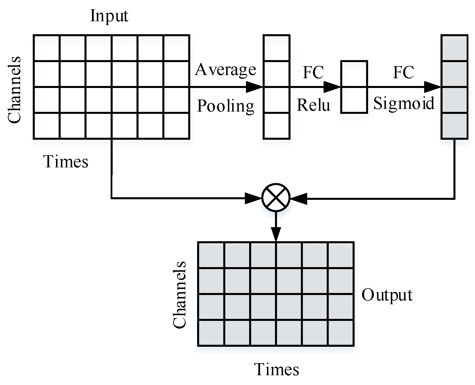
The one-dimensional channel attention mechanism module uses the SE module [17] (Figure 1) to explicitly design the dependencies among different feature channels. The first step is to change the dimensional operation of the input features (Squeeze), where the global average pooling of the space is performed on a feature map (), which means each one-dimensional feature with channel length is pooled into a mean real number and the global feature map () with feature size () is obtained. The -th element can be expressed as:
The second step is to model the correlation among channels through the bottleneck structure composed of two fully connected neural network layers to generate the relevant weight α. The expression of α is of the following form:
In Formula (2), is the weight of the first fully connected layer of the convolution process, which aims to sparse the structure of the model and enhance its generalization ability, ; is the weight of the second fully connected layer of the convolution process, which aims to recover the generalized channel to the original number of channels, ; represents the number of channels, is the hyper-parameter in the training process, generally valued at 8 or 16; represents the sigmoid activation function, which aims to normalize the weights to distribute them between 0 and 1.
The weighted feature map after the output is . The expression of is of the following form:
On the premise of increasing a small amount of computational complexity, the SE module makes the network structure pay more attention to the more important information of fault arc detection in the input item, which has a good effect on improving the performance of network structure.
Based on the SE module, this paper draws on the channel attention module (CAM) proposed by Woo et al. [18]. The structure diagram of CAM is shown in Figure 2.
In the channel attention mechanism module of the CAM mechanism, the main steps are as follows. In the first step, two feature maps are obtained by conducting two operations referred to as ‘Global Max Pooling’ and ‘Global Average Pooling’ on the input feature maps of size , respectively. In the second step, two feature maps are input into a shared neural network (shared MLP), which is composed of two layers of one-dimensional convolutional neural networks with and neurons. The third step is to add the corresponding elements to the two output vectors to obtain a new feature map.
Finally, the weight of the channel attention is obtained by the sigmoid activation function, and then the feature map weighted by the channel attention mechanism is obtained by multiplying it with the elements corresponding to the initial input feature map. The weight value formula in the one-dimensional channel attention mechanism is:
In Formula (4), and are the weights of the fully connected layer in the convolution process; denotes the sigmoid activation function; represents the average pooling feature map; represents the maximum pooling feature map.
The feature map after channel weighting is . The expression of is of the following form:
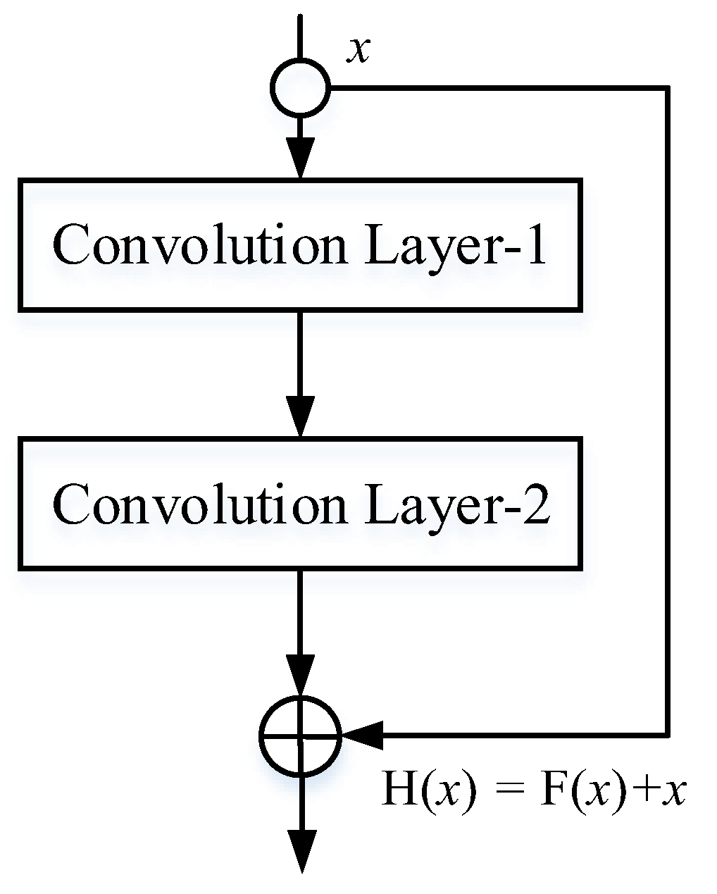
2.2. Residual Neural Network Structure
The structure of a general neural network is connected by neurons in the front and back layers. After receiving the linear mapping of the previous layer, each layer of the neural network will perform a nonlinear activation operation on the output of this layer through the activation function, which connects weights among neurons. The neural network obtains the ability to nonlinearly fit various complex data relationships by this means. In the process of network training, the backpropagation algorithm is generally used, which is based on the gradient descent strategy. In addition, the negative gradient direction of the objective function is used as the benchmark to update the parameters to be trained. It is obvious that when the number of network layers increases, the number of updated parameters will increase rapidly with the phenomenon of gradient explosion.
2.3. Depth Separable Convolution
Depth separable convolution was proposed by Sifre [20]. It was originally applied to the field of image texture classification and achieved good classification results. Chollet [21] proposed the Xception network for the first time to apply depth separable convolution to image classification. The Xception network is based on Inception v3, replacing the Inception module with depth separable convolution, thereby reducing the quantities of parameters of the model and improving the utilization of parameters. Howard et al. [22] proposed the mobile model Mobile-Net using separable depth convolution, which not only reduces the computational complexity but also reduces the size of the model. Therefore Mobile-Net has been widely used in real mobile application scenarios.
The standard convolution realizes the spatial information transmission of feature mapping and the information transmission among channels through one convolution operation. Compared with standard convolution, depth separable convolution divides the process of standard convolution into a depth convolution and a 1 × 1 pointwise convolution. Through the two steps above, the amount of calculation and parameters of the neural network can be reduced, which can improve the operation speed of the model and reduce the size of the model. The contrast between standard convolution and depth-wise separable convolution is shown in Figure 4 and Figure 5.
Figure 5a describes the deep convolution process, which is grouped according to the channel of the input feature map. Figure 5b represents the description of the pointwise convolution process, which is to convolve each group’s channels independently. Compared with quantities of the calculation and parameter in the standard convolution process, the general formulas with respect to quantities of the calculation and parameter in the standard convolution process are shown in Formulas (6) and (7).
In the formulas, is the amount of calculation in the standard convolution process; is the parameter quantity in the standard convolution process; is the number of layers of the convolutional network; is the feature size length of the l-th convolution kernel; is the number of channels output by the layer; is the number of channels output by layer (the number of channels input by layer ).
According to the depth-wise separable convolution visualization map, the general formulas with respect to quantities of the calculation and parameters in the depth-wise separable convolution process can be derived as shown in Formulas (8) and (9).
In the formulas, is the amount of calculation in the depth separable convolution process; is the parameter quantity in the process of depth separable convolution; the ratio of the amount of calculation, the number of parameters in the depth separable convolution and the standard convolution can be obtained by Formulas (10) and (11).
In the formulas, is the ratio of the calculation amount of depth separable convolution and standard convolution; is the ratio of depth separable convolution to standard convolution parameter.
2.4. Arc Fault Detection Network Model Architecture
The method mentioned in this paper combines the advantages of the residual network, one-dimensional convolution channel attention mechanism and depth separable neural network (CA-Model). It improves the accuracy of the neural network model in the process of arc fault prediction, in addition to reducing the quantities of model parameters and floating points. The neural network model used in this method is shown in Figure 6.
In Figure 6, CA-Model mainly includes residual network, one-dimensional channel attention network, one-dimensional depth separable network and prediction network module. The specific parameter settings of the network module are shown in Figure 7.
Figure 7 shows the structure flow chart of a convolutional neural network for arc fault detection. Because the model proposed in this paper has a certain depth and complexity, the diagram is presented in the form of modules. Figure 7b shows the parameter setting of ‘Dw Conv1d_block’. It includes a one-dimensional depthwise separable convolution process with a convolution kernel size of 3 and a step size of 1, a batch normalization layer, and an activation function layer. Figure 7c shows the parameters setting of ‘Resnet_block’. It includes three Dw Conv1d_block. In Figure 7a, Resnet_block2 represents two residual block unit modules, Resnet_block8 represents eight residual block unit modules, Resnet_block4 represents four residual block unit modules, FC represents the fully connected network layer.
3. Experiments and Model Validation
3.1. Arc Fault Detection Experiment
3.1.1. Data Set Establishment
The data set used in this paper is the ‘Intever public database’ for low-voltage series arc fault detection (IAED). The data set contains two different sampling frequencies of current and voltage waveforms and designs a variety of different load connection modes and uses a high-frequency current data set under three different wiring modes. The operating conditions are shown in Figure 8.
Figure 8 shows three different wiring methods used in the experiment. The lines’ devices include an arc generating device, load, 220 V AC power supply, voltmeter, and ammeter. According to the connection mode, it can be divided into the following three types:
- (a)
- The working condition of the arc generator and the single load in series.
- (b)
- The arc generator in series with two loads in parallel.
- (c)
- The arc generator connected in series with two loads in parallel and the connection mode.
The experimental data set uses two wiring methods in Figure 8a,b. Considering that the generation of low-voltage series arc fault is also affected by load type, resistance, inductive load and other factors, the data set is designed with different load types, which can effectively simulate the actual working conditions of arc occurrence. There are six different load configurations, including a microwave oven, induction cooker, electric kettle, electric oven, refrigerator and electric rice cooker.
In the experiment, a 16 bit 10 Khz embedded sensor is used in the high sampling frequency recording process. The current waveforms of the load collected by two different wiring methods are shown in Figure 9. They are: (a) the current diagram of the electric kettle is collected in a single load condition line; (b) the current diagram of the microwave oven and refrigerator in parallel are collected in the mixed load condition line.
Figure 9 shows that the current waveforms during regular operation are all relatively stable sine waveforms. The amplitude of the fault arc current is slightly smaller than the current amplitude in the normal working circuit. The current in the line will have a ‘zero break’ condition near the zero point, so it can be seen from the waveform that there is a ‘prominent flat shoulder’ phenomenon at the zero crossing. In general, the characteristics of arc fault are not prominent, and its identification is difficult.
Table 1 shows the collection time of arc and normal samples for six load configurations under a single load condition line. Table 2 shows the arc sample and average sample collection time of six load configurations in the mixed load condition (‘+’ means that two loads are connected in parallel in the line, and the line is shown in Figure 8b). Since the sampling frequency is 10 Khz, at the same time, the fault arc cycle of a sampling sequence is generally close to five. Therefore, a sampling sequence is about 100 ms.
3.1.2. Sample Data Preprocessing and Parameter Optimization
The normalization of data samples can effectively improve the accuracy of prediction. The maximum and minimum normalization method adopted in this experiment is to normalize the sample data to the interval of (−1, 1). The normalized calculation formula of its minimum and maximum values is of the following form:
In Formula (12), is the normalized sample data; and are the maximum and minimum values in the sample sequence, respectively; and are the right and left endpoints of the normalized interval, respectively.
The experimental prediction model is selected as . is the current data sequence within the -th sampling point and is the probability of arc occurrence through the -th sampling of the prediction model. is the predicted value obtained by the neural network, and the mean square error between the actual value and the predicted value is used as the loss function . The formula is of the following form:
In the formulas above, is the mapping function of neural network; is the total amount of sample data; is the parameter in the neural network.
In this experiment, the data samples are divided into the training set, verification set and test set according to the ratio of 6:3:1. According to the load type and the working condition of the mixed load, the data are divided into two groups: single load and mixed load. When the arc fault occurs, the voltage waveform change will have a lag. Due to that, the experiment selects the current as the input of the deep neural network. This experiment detects whether the arc fault occurs, which is a binary classification problem. Therefore, the training results are labelled during the experiment: 1 indicates an arc occurrence, and 0 shows no arc occurrence.
3.1.3. Experimental Parameter Settings
Network parameters include training parameters and hyperparameters. The setting of hyperparameters is often through repeated experiments. The appropriate hyperparameters have an important influence on the accuracy of neural network prediction and training time. The hyperparameters of the experiment are set as follows: the learning rate is 0.002; the data window length is 1000; the number of iterations is 100; the channel attention mechanism is 16; and the Adam algorithm is used as the optimizer during training.
The F1 value is used as the evaluation index to quantify the neural network model’s prediction effect. The prediction concerning the occurrence of an arc fault is a binary classification problem. As the most commonly used evaluation index, the F1 value can comprehensively and effectively evaluate the prediction accuracy of the network model when the proportion of positive and negative samples is unknown. The precision is the ratio of the predicted results to the actual positive samples in the positive samples. The higher the accuracy, the stronger the ability of the model to distinguish the negative examples. Its expression is as follows:
The recall rate represents the proportion of positive samples in the actual positive samples. The higher the recall rate, the stronger the model’s ability to distinguish positive samples. Its expression is as follows:
The more significant the F1 value, the better the classification effect of the neural network model. The formula can be derived as follows:
The experimental evaluation model complexity includes the space and time complexity of the model. The index of space complexity is the number of parameters in the model. The number of parameters is the number of weights in the neural network training process. The number of model parameters not only affects the prediction effect but also has a direct relationship with the memory space occupied by the model. To compress the size of the network model, the arc detection is realized on the edge end side. The time complexity index of the model is the number of floating-point operations (FLOPs).
4. Results
4.1. Design of Experimental Hardware Environment
The experiments in this chapter not only deal with a large amount of one-dimensional data but also need to prove the superiority of the network model designed in this paper through comparative experiments of different convolutional neural networks. Therefore, it is necessary to ensure that the hardware conditions of other experiments are the same. The training and testing of this experiment were carried out on an Intel i7-13700K model CPU processor and an NVIDIA RTX 24 GB model GPU processor.
4.2. Analysis of Experimental Results of the Models
Based on the residual network structure, the network model structure of this example is improved by embedding the channel attention mechanism and the one-dimensional depth separable convolution module into the deep residual network structure, which is the one-dimensional depth separable convolution residual network structure (Faster CA-Model) based on the channel attention mechanism proposed in this paper. It is experimentally evaluated under six different loads in single and mixed conditions to verify that the network structure has good prediction performance and generalization ability. The evaluation index of a single working condition is shown in Table 3.
From the analysis of the statistical results in Table 3, the average recognition accuracy under different load conditions is 97.75%; the average evaluation value of F1 is 0.9645. The network structure of this example achieves better prediction results under a single load condition. In addition, when the electric oven is used as a single load condition, its F1 value performs best, reaching 0.9794. It can be seen from the line chart in Figure 10 that the accuracy rate is relatively stable in different working conditions. Moreover, the performance of the F1 value is the most durable, indicating that the network model of this example has better recognition ability for positive and negative samples, and the performance is more robust.
The six load evaluation indexes of mixed conditions are shown in Table 4 (‘+’ means that two loads are connected in parallel in the line, and the line is shown in Figure 8b). As can be seen, the performance of the refrigerator and induction cooker in parallel is the best. In general, the version of the model under single working conditions is better than that under mixed working conditions, which also shows that the model has better prediction performance for arc fault under varied working conditions. It is more effective to solve the problem that the arc characteristics could be more evident and easier to identify under mixed load conditions.
4.3. Algorithm Performance and Model Comparison Analysis
To verify the performance of the channel attention mechanism and the one-dimensional depth separable convolution, the three network models of Basic-Model, CA-Model and Faster CA-Model are compared and analyzed based on the above parameter settings and experimental methods and three data sets of mixed load conditions. The F1 values are shown in Table 5. CA-Model is the residual network structure of the embedded channel attention module; Basic-Model is the basic deep residual network structure; Faster CA-Model is a one-dimensional depth separable network structure based on channel attention mechanism. Compared with the Basic-Model network, the F1 value of the CA-Model is 0.97, which indicates that in the process of arc fault prediction, introducing a channel attention mechanism on the same network architecture can pay more attention to the critical information in the data, thus improving the network’s ability to predict arc fault.
Aiming at the problem of many redundant parameters in the neural network, the example introduces the one-dimensional depth separable convolution module. From Table 5 and Table 6, after introducing one-dimensional depth separable convolution into CA-Model, the floating-point number of the one-dimensional depth separable neural network (Faster CA-Model) based on channel attention mechanism is reduced by 45.74%, and the parameter amount is reduced by 46.06%. At the same time, the average prediction time of each sample is reduced by 6.72 ms. Although the accuracy of the network is slightly reduced after the introduction of one-dimensional depth-wise separable convolution, a more accurate and objective F1 value can still be maintained, which proves that the one-dimensional depth-wise separable convolution network can effectively work in model compression, parameter quantity and time complexity reduction with less loss of accuracy.
To verify the generalization ability and robustness of the algorithm, this paper compares and analyzes the complexity, F1 value, time complexity and generalization performance of the depth separable arc fault detection neural network based on channel attention mechanism in five different neural network structures. Six neural network structures include Basic-Model, CA-Model, Faster CA-Model, CNN, AlexNet and Yolov3.
Under the same working condition, the model is compared with CNN, VGG-11, AlexNet and Yolov3 networks. The detection performance of arc faults with different load settings is also analyzed, and the F1 value is shown in Table 7.
According to the results of Table 7, the F1 value of the model proposed in this paper performs best under nine different working condition data sets (except for the microwave oven working condition). Still, it serves more generally on the microwave oven working condition due to the algorithm proposed in this paper being based on a deep neural network. The learning process is end-to-end, closed, so there is room for improvement. Compared with three external neural networks, CNN, AlexNet, and VGG-11, the network model proposed in this paper increases the number of layers of the network and uses the residual structure to avoid the disappearance and explosion of the gradient. The performance of F1 in nine different load settings is superior to the above three networks, and the induction cooker condition performs best, with its F1 value reaching 97.76%. Compared with the Yolov3 deep neural network, which also uses the residual network, this method adds the channel attention mechanism, which can improve the prediction accuracy of the network model. It is more evident in the electric kettle condition, which increased by nearly 3.85%. However, it performs poorly in washing machine and refrigerator conditions. The reasons and conditions need further research and analysis. Therefore, the network model proposed in this paper performs better in comparing shallow and deep neural networks under different working conditions and has good generalization performance and robustness.
Aiming at the problem that the number of deep layers of the network model brings about many network model parameters, this paper uses a one-dimensional depth separable convolutional neural network. To verify the performance of the network module in reducing parameters and single sample prediction time, six network models are quantitatively compared. The results are shown in Table 8. Compared with the CA-Model, where the one-dimensional depth separable convolution module is added, the parameter amount is reduced by 46.06%. The prediction time of a single sample is 13.89 ms. Since the prediction time of a single sample is much shorter than the time of a sampling sequence, the network model designed in this paper can meet the real-time requirements of fault arc detection. Therefore, the network structure proposed in this paper reduces a large number of parameters and saves a specific sample prediction time under the premise of losing part of the accuracy.
5. Conclusions
In order to identify the series arc fault in a line quickly and accurately, this paper proposes to introduce a channel attention mechanism and one-dimensional depth separable convolution module on the deep residual network structure. The embedded channel attention convolution module is a network that can focus on channels that are more critical for identifying arc faults. The experimental results show that the F1 value of the basic residual network structure is 93.60%, and the F1 value of the CA-Model obtained by embedding the channel attention mechanism is 98.07%, which is improved by 4.47%. This sufficiently shows that the embedded channel attention mechanism improves the detection performance of the network. After introducing the channel attention mechanism, the parameters of the network structure and the time of single sample prediction increase to a certain extent. In order to reduce the model parameters and prediction time, a one-dimensional depth separable convolution module is introduced. On the premise of less loss of accuracy, the parameter quantity is reduced by 46.06%, and the prediction time of a single sample is also saved. Through the comparative analysis of the above multi-index and multi-network, the Faster CA-Model network structure has better fault arc detection performance, generalization ability and robustness and provides the possibility for the application of fault arc detection at the edge end side. However, regardless of the economic cost, the cloud computing platform based on 5G communication technology has a better effect in terms of fault arc prediction accuracy.
Author Contributions
Conceptualization, Y.F. and G.Z.; methodology, Y.F.; validation, Y.L., Y.F., J.Z. and Y.Z.; formal analysis, X.G.; investigation, Y.F.; resources, Y.Z.; writing—review and editing, X.G. All authors have read and agreed to the published version of the manuscript.
Funding
This research was funded by Key-Area Research and Development Program of Guangdong Province under No. 2020B0101130023.
Data Availability Statement
Available upon request.
Acknowledgments
The authors would like to express their gratitude for the valuable recommendations made by the reviewers to improve the quality of this paper.
Conflicts of Interest
The authors declare no conflict of interest.
References
- Hu, A.X. National fire situation in 2020. Fire Prot. 2021, 7, 14–15. [Google Scholar]
- Medora, N.K.; Kusko, A. Arcing faults in low and medium voltage electrical systems: Why do they persist. In Proceedings of the 2011 IEEE Symposium on Product Compliance Engineering Proceedings, San Diego, CA, USA, 10–12 October 2011; IEEE: New York, NY, USA, 2011; pp. 1–6. [Google Scholar]
- Wu, Q.; Zhang, Z.C.; Tu, R.; Yang, K.; Zhou, X.J. Simulation research on steady-state heat transfer characteristics of DC fault arc. J. Electrotech. Technol. 2021, 36, 2697–2709. [Google Scholar]
- Wang, L.D.; Wang, Y. DC fault characteristics of arc and detection methods. China Sci. Technol. Inf. 2021, 06, 86–90. [Google Scholar]
- Zhu, C.; Wang, Y.; Xie, Z.H.; Ban, Y.S.; Fu, B.; Tian, M. Serial arc fault identification method based on improved AlexNet model. J. Jinan Univ. 2021, 35, 605–613. [Google Scholar]
- Zhang, G.Y.; Zhang, X.L.; Liu, H.; Wang, Y.H. On-line detection of series fault arc in low-voltage systems. Electrotech. Sci. 2016, 31, 109–115. [Google Scholar]
- Guo, F.Y.; Gao, H.X.; Tang, A.X.; Wang, Z.Y. Serial fault arc detection and line selection based on local binary mode histogram matching. J. Electrotech. Technol. 2020, 35, 1653–1661. [Google Scholar]
- Saleh, S.A.; Valdes, M.E.; MARDEGAN, C.S.; Alsayid, B. The state-of-the-art methods for digital detection and identification of arcing current faults. IEEE Trans. Ind. Appl. 2019, 55, 4536–4550. [Google Scholar] [CrossRef]
- Garima, G.; Pankaj, K.G. A design analysis and implementation of PI, PID and fuzzy supervised shunt APF at load application to improve power quality and system reliabilit. Int. J. Syst. Assur. Eng. Manag. 2021, 12, 1247–1261. [Google Scholar]
- Dołęgowski, M.; Szmajda, M. A Novel Algorithm for Fast DC Electric Arc Detection. Energies 2021, 14, 288. [Google Scholar] [CrossRef]
- Dolegowski, M.; Szmajda, M. Mechanisms of electric arc detection based on current waveform spectrum and incremental decomposition analysis. Prz. Elektrotechniczny 2016, 92, 59–62. [Google Scholar] [CrossRef]
- Zhang, T.; Wang, H.Q.; Zhang, R.C.; Tu, R.; Yang, K. Arc fault detection method based on self-normalized neural network. J. Instrum. 2021, 42, 141–149. [Google Scholar]
- Yu, Q.F.; Huang, G.L.; Yang, Y.; Sun, Y.Z. A detection method for series arc fault based on AlexNet deep learning network. J. Electron. 2019, 33, 145–152. [Google Scholar]
- Wang, Y.; Hou, L.; Paul, K.C.; Ban, Y.; Zhao, T. ArcNet: Series AC arc fault detection based on raw current and convolutional neural network. IEEE Trans. Ind. Inform. 2021, 18, 77–86. [Google Scholar] [CrossRef]
- Zhu, Z.L.; Rao, Y.; Wu, Y.; Qi, J.N.; Zhang, Y. Research progress of attention mechanism in deep learning. Chin. J. Inf. 2019, 33, 1–11. [Google Scholar]
- Li, Y. Research on Image Super-Resolution Reconstruction Method Based on Deep Learning and Attention Mechanism. Ph.D. Thesis, South China University of Technology, Guangzhou, China, 2019. [Google Scholar]
- Hu, J.; Shen, L.; Sun, G. Squeeze-and-excitation networks. In Proceedings of the IEEE Conference on Computer Vision and Pattern Recognition, Salt Lake City, UT, USA, 18–23 June 2018; pp. 7132–7141. [Google Scholar]
- Woo, S.; Park, J.; Lee, J.Y.; Kweon, I.S. Cbam: Convolutional Block Attention Module. In Proceedings of the European Conference on Computer Vision (ECCV), Munich, Germany, 8–14 September 2018; pp. 3–19. [Google Scholar]
- He, K.; Zhang, X.; Ren, S.; Sun, J. Deep Residual Learning for Image Recognition. In Proceedings of the 2016 IEEE Conference on Computer Vision and Pattern Recognition (CVPR), Las Vegas, NV, USA, 27–30 June 2016. [Google Scholar]
- Sifre, L.; Mallat, S. Rigid-Motion Scattering for Texture Classification. Comput. Sci. 2014, 3559, 501–515. [Google Scholar]
- Chollet, F. Xception: Deep Learning with Depthwise Separable Convolutions. In Proceedings of the 2017 IEEE Conference on Computer Vision and Pattern Recognition (CVPR), Honolulu, HI, USA, 21–26 July 2017. [Google Scholar]
- Howard, A.G.; Zhu, M.; Chen, B.; Kalenichenko, D.; Wang, W.; Weyand, T.; Andreett, M.; Adam, H. Mobile Nets: Efficient Convolutional Neural Networks for Mobile Vision Applications. arXiv 2017, arXiv:1704.04861. [Google Scholar]
Figure 1.
SE module structure diagram.

Figure 2.
CAM module structure diagram.

Figure 3.
Residual unit basic structure diagram.

Figure 4.
One-dimensional standard convolution process.

Figure 5.
One-dimensional depth-wise separable convolution process. (a) Depthwise Convolution; (b) Pointwise Convolution.
Figure 5.
One-dimensional depth-wise separable convolution process. (a) Depthwise Convolution; (b) Pointwise Convolution.

Figure 6.
Schematic diagram of CA-Model structure.

Figure 7.
Network module parameter setting.

Figure 8.
Arc fault experiment circuit diagram. (a) One appliance; (b) Two appliances, load 1 and load 2 are parallelly connected; (c) two appliances, arc is generated on the branch with load 1.
Figure 8.
Arc fault experiment circuit diagram. (a) One appliance; (b) Two appliances, load 1 and load 2 are parallelly connected; (c) two appliances, arc is generated on the branch with load 1.

Figure 9.
The current diagram of arc generation under different working conditions. (a) the current diagram of the electric kettle; (b) the current diagram of the microwave oven and refrigerator in parallel.
Figure 9.
The current diagram of arc generation under different working conditions. (a) the current diagram of the electric kettle; (b) the current diagram of the microwave oven and refrigerator in parallel.

Figure 10.
Line chart of the evaluation index under a single working condition of the network model.
Figure 10.
Line chart of the evaluation index under a single working condition of the network model.


Table 1.
Sample collection time information of different loads under a single working condition.
| Load Types | Fault Arc Sample(s) | Normal Sample(s) |
|---|---|---|
| Microwave Oven | 68.3 | 194.9 |
| Electromagnetic Furnace | 45.2 | 151.8 |
| Electric Kettle | 72.2 | 143.1 |
| Electric Oven | 59.2 | 131.8 |
| Refrigerator | 53.7 | 102.3 |
| Electric Rice Cooker | 62.3 | 113.6 |
Table 2.
Collection time information of arc samples with different loads under mixed conditions.
| Load Types | Fault Arc Sample(s) | Normal Sample(s) |
|---|---|---|
| Microwave Oven + Electric Kettle | 67.8 | 125 |
| Electric Rice Cooker + Electric Oven | 87.7 | 178.7 |
| Refrigerator + Electromagnetic Furnace | 72.7 | 247.5 |
Table 3.
Evaluation index of Faster CA-Model network under a single working condition.
| Load Types | Recall | Precision | F1 | Accuracy |
|---|---|---|---|---|
| Microwave Oven | 0.9432 | 0.9863 | 0.9643 | 0.9794 |
| Electromagnetic Furnace | 0.9649 | 0.9632 | 0.9747 | 0.9834 |
| Electric Kettle | 0.9346 | 0.9823 | 0.9579 | 0.9786 |
| Electric Oven | 0.9786 | 0.9802 | 0.9794 | 0.9832 |
| Refrigerator | 0.9564 | 0.9769 | 0.9665 | 0.9896 |
| Electric Rice Cooker | 0.9413 | 0.9632 | 0.9521 | 0.9565 |
Table 4.
Evaluation index of Faster CA-Model network under mixed load conditions.
| Load Types | Recall | Precision | F1 | Accuracy |
|---|---|---|---|---|
| Microwave Oven + Electric Kettle | 0.8844 | 0.9214 | 0.9026 | 0.9348 |
| Electric Rice Cooker + Electric Oven | 0.9432 | 0.9863 | 0.9643 | 0.9794 |
| Refrigerator + Electromagnetic Furnace | 0.9767 | 0.9843 | 0.9806 | 0.9875 |
Table 5.
Comparison of F1 values of different models under mixed load conditions.
| Network Model | Microwave Oven Electric Kettle | Electric Rice Cooker Electric Oven | Refrigerator Electromagnetic Furnace |
|---|---|---|---|
| Basic-Model | 0.9360 | 0.9769 | 0.9543 |
| CA-Model | 0.9807 | 0.9889 | 0.9693 |
| Faster CA-Model | 0.9617 | 0.9805 | 0.9617 |
Table 6.
Comparison of experimental results of different network models.
| Quantitative Index | Basic-Model | CA-Model | Faster CA-Model |
|---|---|---|---|
| Flops (M) | 44.81 | 45.31 | 24.58 |
| Parameters (M) | 23.22 | 22.45 | 12.12 |
| Times (ms) | 18.57 | 16.74 | 13.89 |
Table 7.
Comparison of the F1 value of the network model under different working conditions.
| Load Types | Faster CA-Model | CNN | VGG-11 | AlexNet | Yolov3 |
|---|---|---|---|---|---|
| Microwave Oven | 0.9143 | 0.8671 | 0.8896 | 0.8642 | 0.9332 |
| Electromagnetic Furnace | 0.9776 | 0.9026 | 0.8649 | 0.8762 | 0.9456 |
| Electric Kettle | 0.9736 | 0.9145 | 0.9441 | 0.9012 | 0.9351 |
| Electric Oven | 0.9623 | 0.8956 | 0.9123 | 0.9423 | 0.9521 |
| Refrigerator | 0.9457 | 0.8836 | 0.9216 | 0.8612 | 0.9432 |
| Electric Rice Cooker | 0.9633 | 0.8765 | 0.8921 | 0.9063 | 0.9612 |
| Microwave Oven + Electric Kettle | 0.9617 | 0.8469 | 0.8346 | 0.8936 | 0.8963 |
| Electric Rice Cooker + Electric Oven | 0.9805 | 0.8934 | 0.9025 | 0.9321 | 0.9452 |
| Refrigerator + Electromagnetic Furnace | 0.9617 | 0.8701 | 0.8435 | 0.8865 | 0.9601 |
Table 8.
Quantitative comparison of contrasting network models.
| Network Model | Flops (M) | Parameters (M) | Times (ms) |
|---|---|---|---|
| Faster CA-Model | 24.58 M | 12.12 M | 13.89 |
| CNN | 10.25 M | 6.23 M | 15.93 |
| VGG-11 | 52.63 M | 26.78 M | 26.41 |
| AlexNet | 32.52 M | 16.23 M | 12.36 |
| Yolov3 | 44.85 M | 23.22 M | 18.57 |
Disclaimer/Publisher’s Note: The statements, opinions and data contained in all publications are solely those of the individual author(s) and contributor(s) and not of MDPI and/or the editor(s). MDPI and/or the editor(s) disclaim responsibility for any injury to people or property resulting from any ideas, methods, instructions or products referred to in the content. |
© 2023 by the authors. Licensee MDPI, Basel, Switzerland. This article is an open access article distributed under the terms and conditions of the Creative Commons Attribution (CC BY) license (https://creativecommons.org/licenses/by/4.0/).
Share and Cite
MDPI and ACS Style
Gao, X.; Zhou, G.; Zhang, J.; Zeng, Y.; Feng, Y.; Liu, Y. Fault Arc Detection Based on Channel Attention Mechanism and Lightweight Residual Network. Energies 2023, 16, 4954. https://0-doi-org.brum.beds.ac.uk/10.3390/en16134954
AMA Style
Gao X, Zhou G, Zhang J, Zeng Y, Feng Y, Liu Y. Fault Arc Detection Based on Channel Attention Mechanism and Lightweight Residual Network. Energies. 2023; 16(13):4954. https://0-doi-org.brum.beds.ac.uk/10.3390/en16134954
Chicago/Turabian StyleGao, Xiang, Gan Zhou, Jian Zhang, Ying Zeng, Yanjun Feng, and Yuyuan Liu. 2023. "Fault Arc Detection Based on Channel Attention Mechanism and Lightweight Residual Network" Energies 16, no. 13: 4954. https://0-doi-org.brum.beds.ac.uk/10.3390/en16134954
Note that from the first issue of 2016, this journal uses article numbers instead of page numbers. See further details here.