A Reliability-Optimized Maximum Power Point Tracking Algorithm Utilizing Neural Networks for Long-Term Lifetime Prediction for Photovoltaic Power Converters

Abstract

The reliability of power converters in photovoltaic systems is critical to the overall system reliability. This paper proposes a novel active thermal-controlled algorithm that aims to reduce the rate of junction temperature increase, therefore, increasing the reliability of the device. The algorithm works alongside a normal perturb and observe maximum power point tracking algorithm, taking control when certain temperature criteria are met. In conjunction with a neural network, the algorithm is applied to long-term real mission profile data. This would grant a better understanding of the real-world trade-offs between energy generated and lifetime improvement when using the proposed algorithm, as well as shortening study cycle times. The neural network, when applied to 365 days of data, was 28 times faster than using standard electrothermal modeling, and the lifetime consumption was predicted with greater than 96.5% accuracy. Energy generated was predicted with greater than 99.5% accuracy. The proposed algorithm resulted in a 3.3% reduction in lifetime consumption with a 1.0% reduction in the total energy generated. There is a demonstrated trade-off between lifetime consumption reduction and energy-generated reduction. The results are also split by environmental conditions. Under very variable conditions, the algorithm resulted in a 4.4% reduction in lifetime consumption with a 1.4% reduction in the total energy generated.

1. Introduction

In 2021, the Intergovernmental Panel on Climate Change published the AR6 report, which stated that humans have had an “unequivocal” influence on warming the planet [1] and predicts the global temperature rise to exceed 1.5 ${}^{°}$C above pre-industrial levels before 2050 unless action is taken [2]. Presently, there is a virtual certainty that extreme weather events have increased in both frequency and intensity due to human influence, and there is high confidence that this trend will be exacerbated with rising temperatures. To curtail the temperature increase to 1.5 ${}^{°}$C, it is imperative to achieve substantial emission reduction across all sectors. In the context of the United Kingdom, the government has made a commitment to attain a net-zero greenhouse gas emission target by 2050 [3].

The UK’s Climate Change Committee projects that between 50–75% of the UK’s total energy production will come from variable renewables, including solar photovoltaic (PV) energy, by the year 2050. The generation capacity of solar PV panels, which was 14 GW in 2022, is expected to grow significantly to a range of 145–615 GW [4,5]. Ensuring solar PV energy’s substantial contribution to decarbonizing power generation requires continuous development and improvement in PV technology.

To ensure the maximum energy production from PV panels and offset the manufacturing cost, trade-offs are often made at the expense of system reliability [6]. PV arrays typically endure harsh environmental conditions, including high temperatures, vibrations, and high humidity. Among various stressors, thermal factors are deemed most critical for PV power converters, leading to losses and power cycling [7,8]. According to a survey involving industry experts, 40% of respondents identified power semiconductors as the key area for research to enhance power electronics reliability, highlighting their significance in this context. Notably, a large-scale PV plant operational over five years in Tucson, AZ, USA, experienced 37% of the unscheduled maintenance events related to inverters, accounting for 59% of unscheduled maintenance costs [9]. The survey respondents expressed a collective desire for more research into active methods aimed at improving system reliability.

Active thermal control (ATC) is utilized as an active method for reducing the damage accumulated from thermal cycling, with several techniques being suggested within the power electronic research [10]. An important part of ATC methods in power electronics is an accurate estimation of the junction temperature. Andresen et al. [11] give a review of the current temperature measurement and estimation techniques, and several implementation possibilities for ATC are described. The ATC methods discussed apply to power semiconductors in all applications, rather than specifically grid-connected PV panels. The authors in [12] also provide an overview of the junction temperature measurement and estimation techniques. Some of the literature uses temperature-sensitive electrical properties for temperature estimation [13]. For example, Xu et al. [14] proposed a method whereby the IGBT current is measured during a short circuit pulse, with the short circuit current being directly linked to the junction temperature. The results showed a good ability to predict and calculate temperature; however, this method requires additional hardware for measurement. In their work, Motto and Donlon [15] incorporated temperature sensing directly into a power module by utilizing the forward voltage drop across multiple diodes that were integrated into the semiconductor diode itself. By exploiting the linear relationship between the forward voltage drop and diode temperature, they successfully estimated the junction temperature. However, this implementation resulted in increased module complexity as a trade-off.

Analytical electrothermal models are also used widely within the literature to predict temperature, without the need for measurement hardware [6,16,17]. In [16], the system-level reliability and lifetime prediction of grid-connected PV systems were discussed, for which an electrothermal model is employed. A rainflow counting algorithm is used to find temperature cycles from the electrothermal model, with cycles to failure calculated using the Coffin–Manson law. This procedure is common and well-documented within the literature.

A “lifetime-optimized” perturb and observe (P&O) maximum power point tracking (MPPT) algorithm is proposed in [6], which works to reduce thermal stress during highly variable conditions and limits the power semiconductor junction temperature in PV systems. The results showed the lifetime was improved by 13% while sacrificing 3.7% of potential energy generation when the proposed algorithm was employed. Different parameters were tested, which demonstrated a direct trade-off between energy generation and lifetime reduction. However, the mission profile is not field data and was created based upon the analysis of real irradiance data rather than directly using real irradiance data. Additionally, simulations were only run on a mission profile lasting 10 min.

A similar concept is also presented in [18]. A look-up table was trained on the simulation data and then applied to four days of different environmental conditions. The outcome was an algorithm that improved lifetime by 4.6% while sacrificing 0.02% of total generation. With an accuracy of 95.3%, it is possible, however, that this result is statistically insignificant. Additionally, with just one day of data in each environmental condition category, reliable long term predictions cannot be made. In [19], a statistical approach for IGBT failure analysis is used after electrothermal modeling of a PV system. This is based on Monte Carlo simulations, as physical tolerances and operational stresses vary by component. Probability distribution functions for key electrical and lifetime model parameters are used to find the sensitivity to the accumulated damage. A statistical lifetime analysis is then performed, giving a lifetime with a specified confidence level. The paper discusses changing the electrothermal parameters, such as thermal resistance as the device ages, as is carried out in [20].

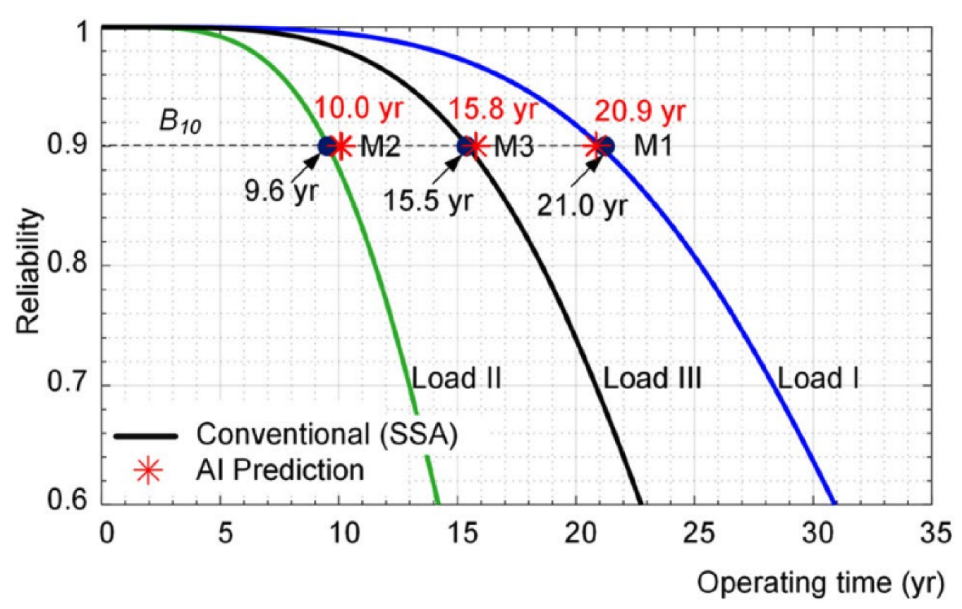
Peyghami et al. [21] introduces a novel power converter lifetime performance indicator, employing an artificial neural network (ANN) to replace the detailed electrothermal model. The paper addresses the lack of easily available long-term reliability performance indicators, allowing for better reliability-orientated design and maintenance planning. Examples of the effect of different mission profiles on the lifetime of the converters and their estimation using the detailed electrothermal-based model and the proposed AI approach are shown in that paper and also given here in Figure 1 for reference.

A Monte Carlo reliability analysis is performed to estimate the $B_{10}$ lifetime of the converter, similar to [19]. The use of ANNs decreased the required time for the lifetime calculation by a factor of 5. Converter electrothermal modeling is used to train the ANN, and the lifetime predictions are found by applying the neural network to a converter mission profile. The ANN could accurately predict the lifetime of a converter with less than a 5% error compared to the traditional stress–strength analysis. However, this paper considers a general power converter under a given constant load rather than, specifically, power converters in a PV system. As a result, with a PV system of varying power generation levels, the same analysis cannot be replicated.

The comparison of the literature studies is shown in

Table 1. Summary of Recent Research Papers on the Reliability of Power Converters.

Year	Ref.	Techniques/Methods/Applications	Contributions	Limitations	Recommendations
2023	[22]	Multivariate-LSTM model, RUL prediction in superbuck converter	Provides early warning of failure and ensures reliable and safe operation in mission-critical applications.	Uses k-fold cross technique and LTSPICE simulation for validation.	Explore more diverse datasets for further validation.
2023	[23]	Mission Profile Based Reliability Analysis, Grid-connected Solar PV-Battery	Compares lifetime of whole system in different configurations and determines AC link configuration to be more reliable.	Lack of real-world data from extreme conditions.	Further investigations into the impacts of environmental factors.
2023	[24]	ANN-fuzzy MPPT controller, Solar PV	Uses AI-based MPPT algorithms and outperforms other controllers in tracking accuracy.	Limited analysis of controller robustness under faults.	Investigate the effect of uncertainties in weather forecasts.
2022	[25]	Reliability assessment models, DC-DC converters	Provides component-level and system-level reliability assessment using different tools.	Component-level data availability varies among manufacturers.	Develop a standardized method for accelerated lifetime testing.
2022	[18]	MPPT algorithm, Grid-connected Solar PV	Introduces a temperature-controlled MPPT algorithm for lifetime improvement of PV converters.	Increased computational complexity due to lookup tables.	Optimize lookup table size for a balance between accuracy and computation time.
2022	[26]	Machine learning applications, Solar PV systems	Explores the use of ML in various aspects of PV systems.	Limited real-world deployment of ML-based controllers.	Implement ML algorithms on field-deployed PV systems for real-world performance evaluation.
2022	[27]	Intelligent Gate Drivers, Future Power Converters	Introduces intelligent gate drivers with active switching control and sensing capabilities for safe operation and thermal management of power devices.	Requires additional sensors for sensing capabilities.	Investigate cost–benefit trade-offs for the implementation of intelligent gate drivers.
2021	[28]	Comparison of Different MPPT Techniques, Various PV applications	Compares various MPPT techniques based on their performance and characteristics.	Limited testing scenarios representing extreme weather conditions.	Conduct experiments in harsh environments to assess performance robustness.
2020	[29]	Thermal Performance Improvement, Multi-Megawatt Power Converters	Implements a carrier-based active thermal control method for temperature regulation in power semiconductor devices.	Focused on a specific converter type, limited to other converter topologies.	Investigate the applicability of the proposed method for other converter topologies.
2020	[30]	Two-level reliability framework, Power converters and systems	Presents a hierarchical reliability framework bridging power converters and power systems.	Limited data availability for some components.	Collect more data to improve the reliability model accuracy.
2019	[31]	Design optimization, Solar PV systems	Provides a comprehensive overview of design optimization techniques for PV systems.	Limited focus on the impact of module-level design on system performance.	Investigate the interaction between module-level design and overall system performance.
2018	[32]	FPGA implementation, reliability and Unified power quality conditioner	Proposes an FPGA-based UPQC system for reliability and power quality improvement in distribution networks.	Evaluation limited to a specific distribution grid topology.	Validate the UPQC system performance on various distribution grid layouts.
2017	[33]	Comparison of control techniques, Grid-connected inverters	Compares various control techniques for grid-connected inverters based on their performance and capability.	Limited study on control strategies’ impact on inverter efficiency.	Investigate the trade-offs between control strategies and inverter efficiency.

. Upon summarizing the aforementioned literature, the following observations regarding the limitations in the previous studies were identified:

• The current research in the area of grid-connected PV power converter reliability implement look-up tables to shorten computation times. The accuracy of results is dependent on the size of the look-up table, which is often less than can be achieved with other methods.
• Furthermore, the current literature often uses mission profile data that are not composed of real environmental data.
• Additionally, simulations of a short duration are used that do not accurately show the results over a long period of time and do not reflect the true results if the systems were implemented in the field. As a result, the current research in this area is lacking reliable, transferable information out of simulations with regard to the design for reliability studies.
• Although the proposed multivariate-LSTM model showed better reliability predictions with higher accuracy compared to other deep learning models, there is a need for more diverse and comprehensive datasets to improve the generalizability of the model.
• During the comparison of the lifetime of a grid-connected solar PV system in AC link and DC link configurations, the comparison was based on specific load, mission profile, and the energy management system. Studies should consider a wider range of scenarios to provide more comprehensive insights into reliability differences.
• For an ANN-fuzzy MPPT controller for solar PV systems, the introduction of fuzzy logic increased the complexity of the controller.
• For the reliability assessment models for DC-DC converters, the FIDES model showed a better reliability performance compared to other techniques; it was noted that FIDES is complex in terms of computing. The research could focus on simplifying the computational process without compromising accuracy.
• For a temperature-controlled MPPT algorithm for grid-connected solar PV systems, there is a need for modifications and improvements to the existing MPPT approaches.
• For the application of machine learning (ML) techniques in solar PV systems, the main observation is the need for more open datasets with real data from PV systems to facilitate automatic learning processes.
• For the adoption of intelligent gate drivers for future power converters, there is a need for the widespread adoption of intelligent gate drivers in industrial practice.
• For thermal performance improvement in multi-megawatt power converters, one limitation identified is the high thermal stress experienced by the rotor side converter. The research could explore methods to reduce thermal stress and improve the efficiency and reliability of RSC.

Main Contributions

The main contributions of this paper can be summarized as:

• In order to tackle the aforementioned concerns raised in the existing literature, this paper aims to apply a neural network to a novel active thermal control MPPT algorithm trained using electrothermal models. The novel active thermal control MPPT algorithm presented in this paper aims to further develop the ideas existing within the present research, as well as increase lifetime without significantly negatively impacting power generation.
• The second novel aspect of this paper is to implement a neural network to estimate lifetime, allowing for long-term environmental datasets to be used without extensive and time-consuming simulations and without significantly compromising accuracy. This would grant more reliable data for design for reliability studies, such as a better understanding of real-world trade-offs between energy generated and lifetime improvement when using the ATC algorithm, as well as shortening study cycle times.

The rest of the paper is organized as follows: in Section 2, the PV electrothermal model is described, and the theory governing the power converter lifetime is given. Section 3 describes the method whereby neural networks are implemented in a way to circumvent extensive electrothermal simulations. In Section 4, an active thermal control algorithm is proposed. Section 5 discusses the implementation and details of the PV electrothermal model and neural network training. Finally, Section 6 presents the results of the study.

2. Electrothermal Lifetime Modeling

This section details the theory behind simulating an electrothermal PV model and converting temperature readings into device lifetime consumption values. As shown in [7,8,9], power converters are often the most unreliable components in grid-connected PV systems.

2.1. Electrothermal Modeling

Connecting an inherently DC PV system to the grid can be achieved in many ways [6,20,34]. The differences in implementation result from the level of control and complexity desired. However, most structures use an MPPT-controlled DC/DC stage, with a DC/AC stage connected to the grid. This paper considers a simple structure that has been documented well within the literature.

A 2-stage, single-phase, transformerless grid-connected PV system is used in this paper. The topology can be seen in Figure 2. The first stage is a boost converter controlled by an MPPT algorithm for maximum power extraction. The second stage is a full-bridge grid-connected inverter, which maintains the DC link voltage and exports AC power to the grid, at the correct voltage and phase angle. An LCL filter ensures the output grid current reaches a total harmonic distortion of less than 5% [35].

The power loss in the IGBT is calculated using Equation (1), where the total power loss is the sum of the conduction ($P_{cond}$) and switching ($P_{sw}$) losses. The conduction losses are calculated with collector–emitter voltage $V_{ce}$, collector current $I_c$ and duty cycle D. The switching losses are calculated with switching frequency $f_{sw}$, energy loss during turn on $E_{on}$ and turn off $E_{off}$ [36].

$$P_{total}=\underset{P_{cond}}{\underbrace{V_{ce}·I_c·D}}+\underset{P_{sw}}{\underbrace{f_{sw}·(E_{on}+E_{off})}}$$

(1)

The power loss in the diode is calculated using Equation (2). Similarly to IGBTs, the power loss is split into conduction and switching losses. Conduction losses are based on the forward bias voltage $V_F$, forward current $I_F$ and resistance $R_D$. Switching losses are calculated with reverse recovery charge $Q_{RR}$ and reverse bias voltage $V_R$ [37,38].

$$P_{loss}=\underset{P_{cond}}{\underbrace{V_F·I_{F,avg}+R_D·I_{F,rms}^2}}+\underset{P_{sw}}{\underbrace{\frac{f_{sw}·Q_{RR}·V_R}{3}}}$$

(2)

The semiconductor junction temperature is the temperature of the semiconductor material within the transistor. In this paper, the junction temperature is analyzed as it is a direct contributor to device degradation and failure. However, measuring this temperature is non-trivial. Section 1 gives an overview of the current temperature measurement techniques. For the analysis in this paper, a Foster thermal model is employed to find junction temperatures, with the structure shown in Figure 3 [39]. The Foster thermal models have been applied multiple times within the literature, and while they may not provide a direct link to reality as the Cauer thermal models, they are much easier to implement [6,16,17].

IGBT and diode Foster thermal model values are provided by the IGBT manufacturer. Thermal interface material (TIM) and heatsink values are taken from parts.

2.2. Lifetime Consumption Estimation

This section details the procedure used for estimating the device lifetime consumption based on the junction temperature data. This method has been well documented in literature, especially in conjunction with an electrothermal model [6,10,19,20].

Figure 4 shows short term temperature cycling. It is primarily due to the line frequency, a result of the sinusoidal currents flowing through the inverter; therefore, it typically occurs on a scale less than 1 s. Long-term temperature cycling, on the scale of a few seconds and greater, generally results from irradiance or ambient temperature changes.

The junction temperature samples from the electrothermal model are first analyzed by finding the peaks and valleys, as seen in Figure 5. This removes a lot of the unnecessary data, reducing the required computation for the next stage. A rainflow counting algorithm is then used, which will extract the temperature cycle amplitude, average cycle temperature and cycle count. These data can be used in estimating the number of cycles to failure, described by Equation (3). This equation, described in [40], encompasses many IGBT failure mechanisms.

$$N_f=K·\Delta T_j^{{\beta }_1}·exp\left(\frac{{\beta }_2}{T_j+273}\right)·t_{on}^{{\beta }_3}·I^{{\beta }_4}·V^{{\beta }_5}·D^{{\beta }_6}$$

(3)

where K is a constant term, $t_{on}$ is the heating time, I is the current per bond wire, V is the voltage class of IGBT, and D is the diameter of the bond wire. The temperature swing $\Delta T_j$, absolute temperature $T_j$ and $t_{on}$ can be seen in Figure 5. The model parameters ${\beta }_1$ to ${\beta }_6$ used in this paper are given in [40].

The accumulated lifetime consumption (LC) of the power converter can then be calculated using the Miner’s rule [41]:

$$LC=\sum _i\frac{n_i}{N_{fi}}$$

(4)

where $n_i$ is the number of thermal cycles, and $N_{fi}$ is the expected cycles to failure, calculated in Equation (3). The output, lifetime consumption (LC), is the sum of the damages from each cycle. When LC surpasses 1, the device is predicted to have reached the end of its life. This model does not take into account statistical failure mechanics or the increase in thermal resistance $R_{th}$ with device degradation.

Using the procedure outlined in this section, Section 3 describes the implementation of a regression neural network for the prediction of lifetime consumption values, removing the requirement for the electrothermal modeling described in this section.

3. Neural Network Regression of Lifetime Consumption

Neural networks are mathematical abstractions that mimic the human brain. Their structure can be adjusted to optimize various computational tasks, such as numerical prediction or classification. Regression neural networks, commonly used for making numerical predictions, are prevalent tools in handling non-linear functions. In the context of similar lifetime predictions, neural networks have been successfully applied [21]. An alternative method for estimating lifetime involves the use of look-up tables. However, the accuracy of such an approach is limited by the size of the look-up table [6]. To address this limitation, neural networks are proposed as a method for lifetime consumption prediction. This approach reduces the need for extensive long-term electrothermal modeling while achieving higher accuracy compared to look-up tables.

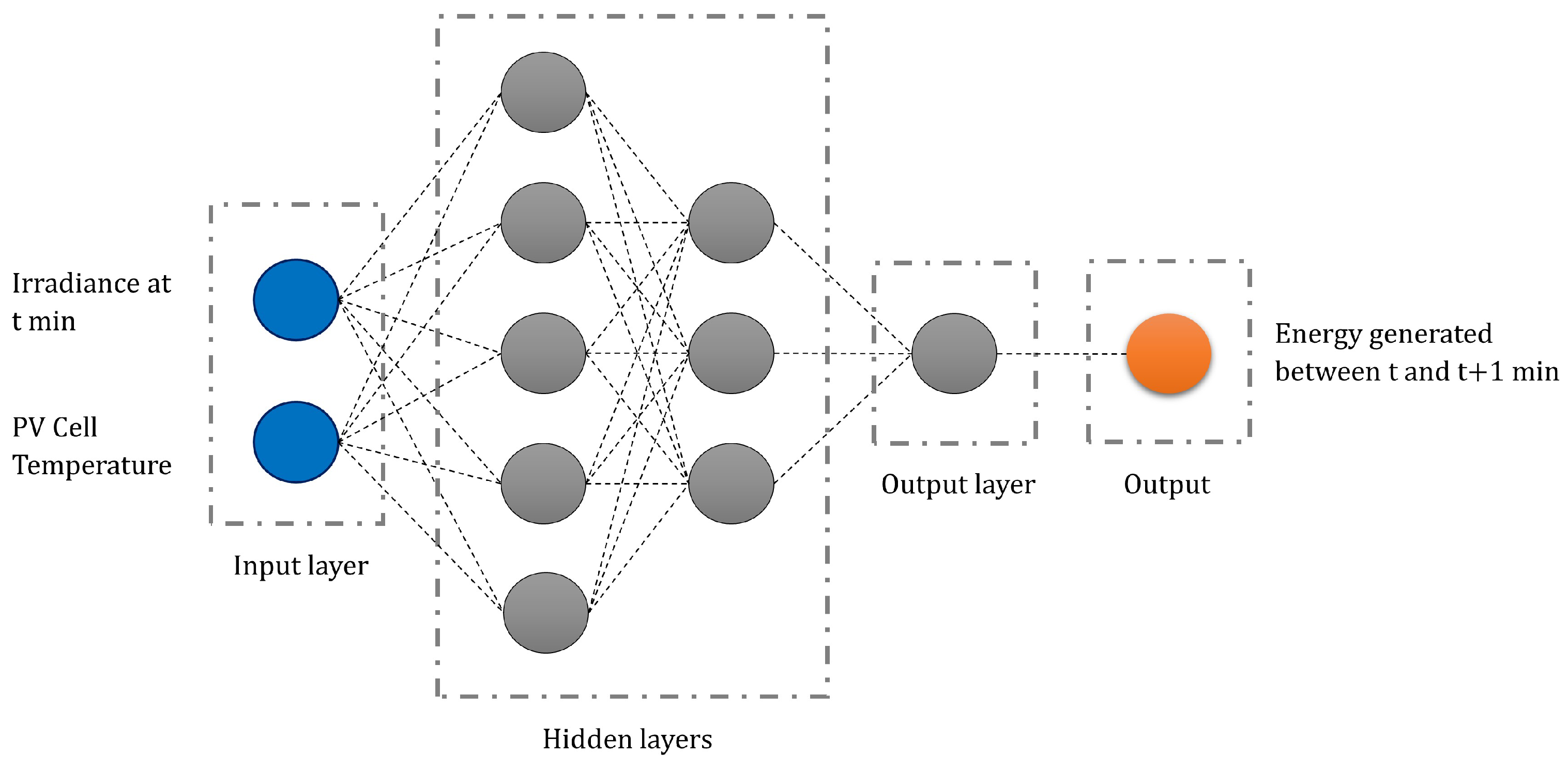
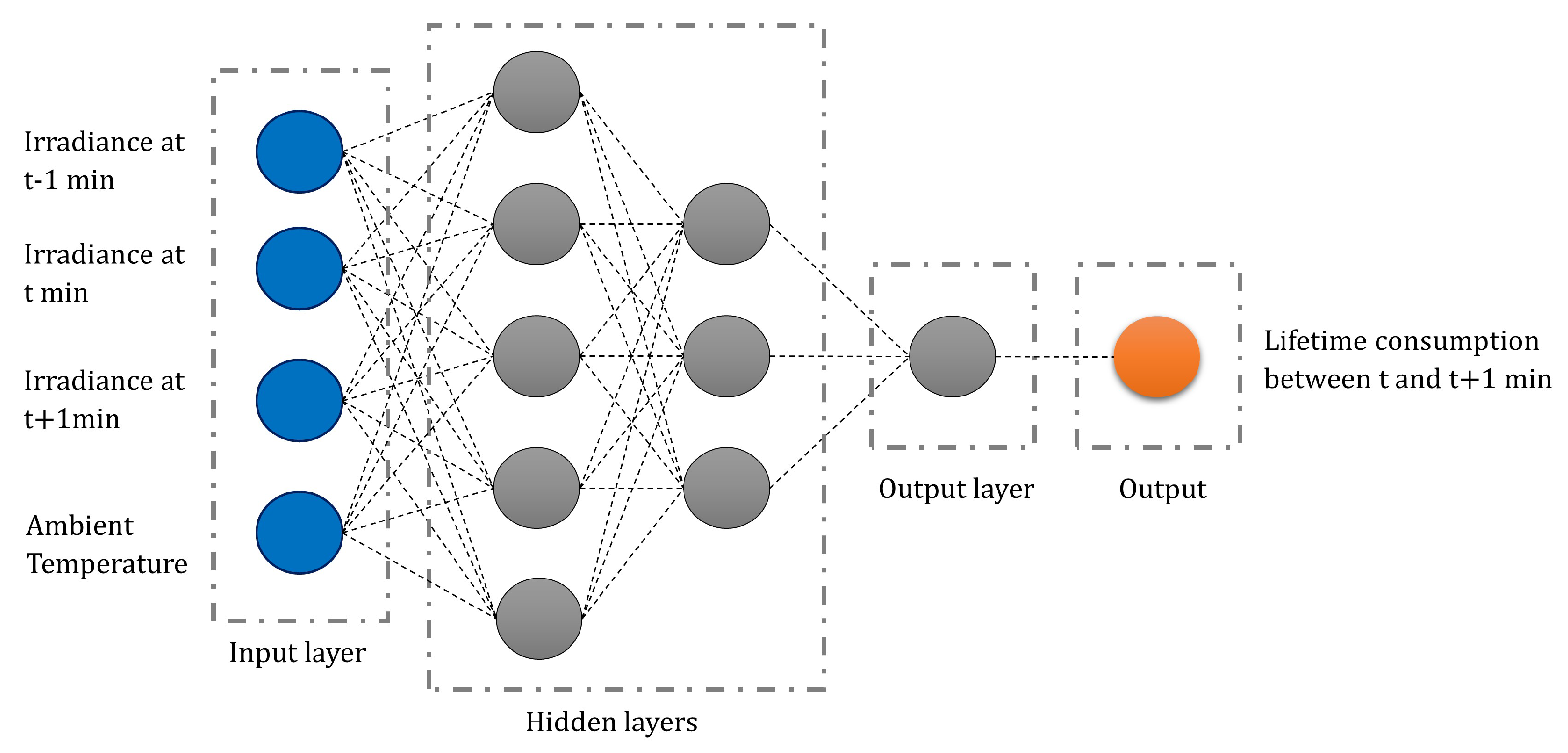
For this work, regression networks were implemented in MATLAB using fitrnet. Fitrnet trains a feed-forward, fully connected neural network designed for regression. Two separate neural networks were used, estimating energy generation (EG) and lifetime consumption (LC). A single multiple output neural network was found to be inaccurate, as network training performance metrics could not train a network accurately for multiple outputs as energy generation is comparatively easier to predict than lifetime consumption, which biased the performance metric. The structure of the neural networks used can be seen in Figure 6 and Figure 7.

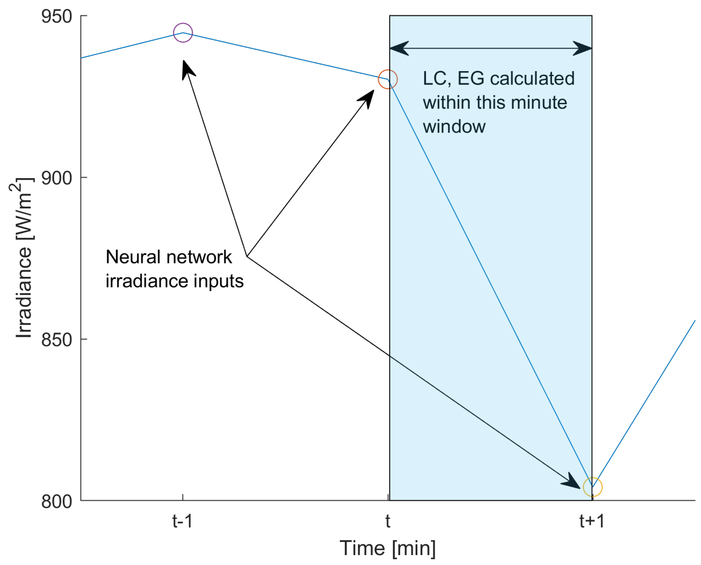
The environmental data used are sampled at a rate of once per minute. A moving window is used that predicts the energy generation and lifetime consumption within the next minute. This is shown in Figure 8. This allows the network to be applied to days of any length, days of interrupted data, as well as reducing the total amount of inputs, consequently reducing computation.

Energy generation in the next minute is predicted using the current irradiance value and cell temperature. Lifetime consumption in the next minute is predicted using the current irradiance, ambient temperature, as well as irradiance values for the minutes on either side. The reasoning for lifetime consumption inputs is focused on the junction temperature. The heat capacitance of the device and heatsink means the junction temperature is not only a function of the current irradiance but also the previous and next irradiance values.

The hidden layer structure was found through trial and error. Other network parameters such as regularization, standardization and activation function were found through hyperoptimization.

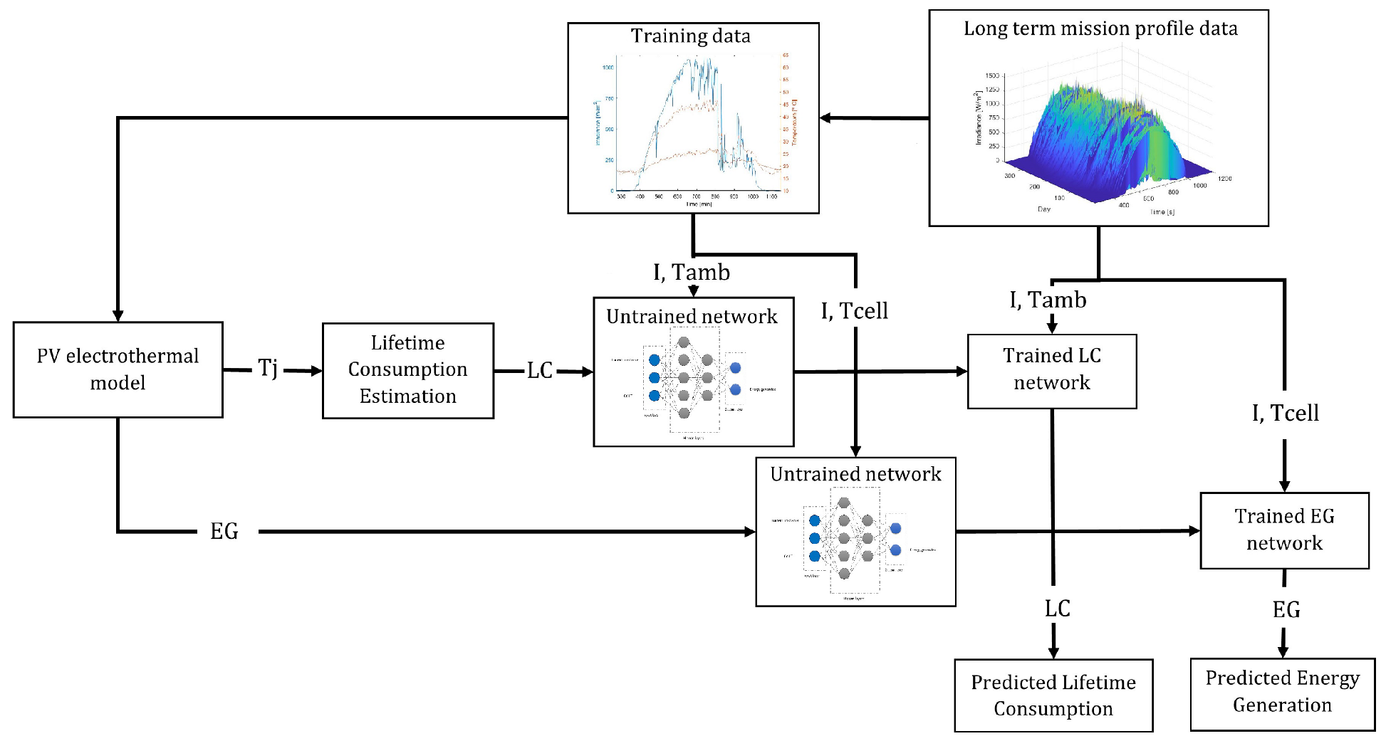
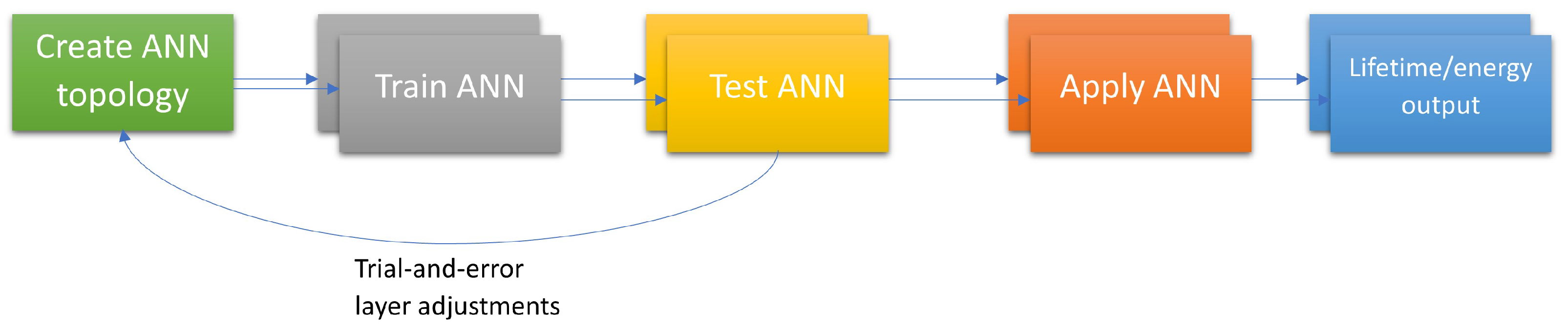
The workflow for the data, showing the process of training and applying neural networks, is shown in Figure 9, with a simplified diagram in Figure 10. The training data represent a selected sample of the long term mission profile data used to train the networks. The training of the networks requires input and target values. The target values are the output of the electrothermal model. The input values are the same inputs to the electrothermal model. Once the networks are trained, they can be applied to long term mission profile data directly, skipping the electrothermal modeling step.

Now that the tools for the prediction of long-term lifetime consumption and energy generation have been described, Section 4 proposes an algorithm for reducing lifetime consumption.

4. Novel Active Thermal Control Algorithm

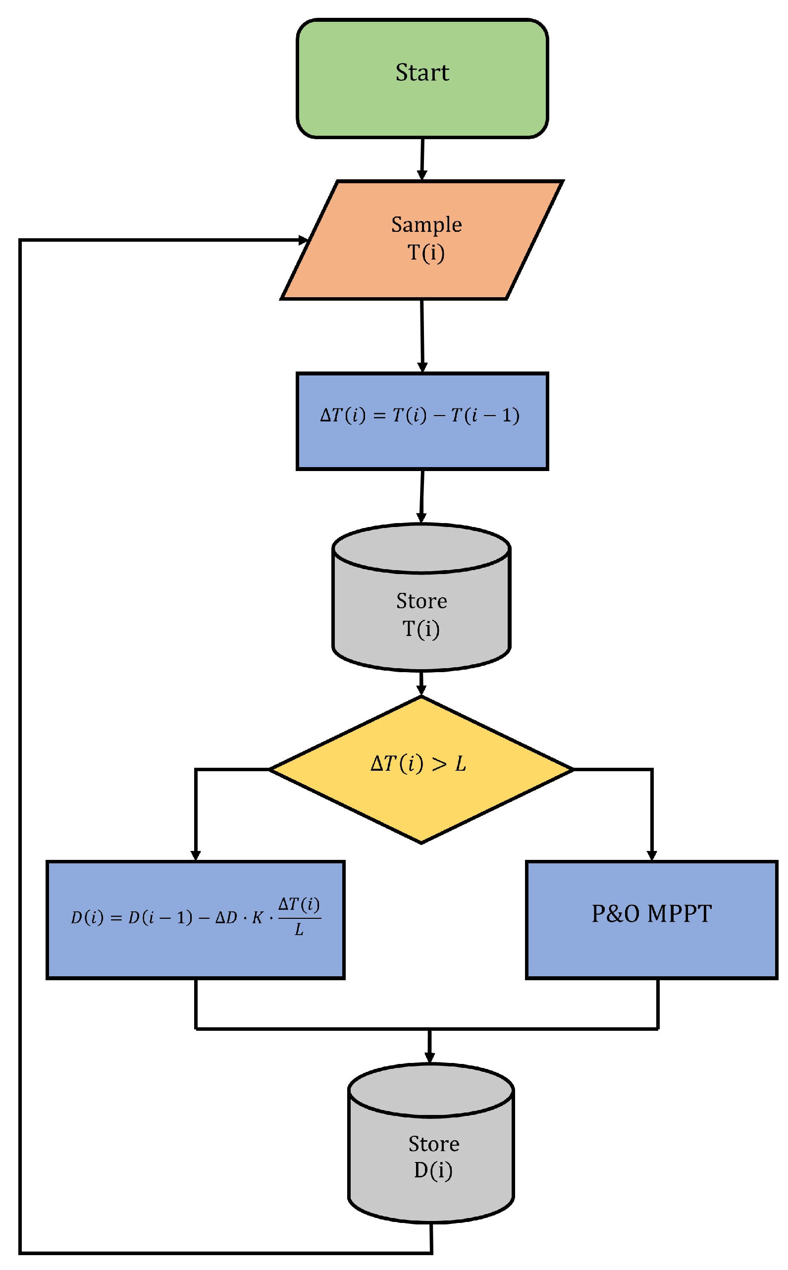
Active thermal control algorithms have become a more important area of research as the industry aims to maximize energy capture and approach device limits [10]. This paper proposes a novel ATC algorithm that works alongside an unchanged P&O MPPT algorithm. The novel ATC aspect takes control when certain temperature criteria are met.

Under normal conditions with no large fluctuations in average junction temperature, the standard P&O MPPT algorithm applies. Once the average junction temperature rise exceeds a defined threshold, the boost converter duty cycle is reduced according to the junction temperature rise, using Equation (5). The algorithm flowchart is seen in Figure 11.

$$D\left(i\right)=D(i-1)-\Delta D·K·\frac{\Delta T_j\left(i\right)}{L}$$

(5)

This equation is designed to decrease the current duty cycle by a value proportional to the ratio that the temperature rise $\Delta T_j$ exceeded the set limit L. L represents the temperature rise limit in ${}^{°}$C/s. A constant term K allows for more control over the magnitude of duty cycle adjustments. The influence of K is shown in Figure 12. $\Delta D$ is the magnitude change of the duty cycle per time-step in the standard P&O MPPT algorithm and is used as a scaling factor. With $K·\Delta T_j/L=1$, the ATC algorithm reduces the duty cycle by the same amount as an unchanged P&O algorithm.

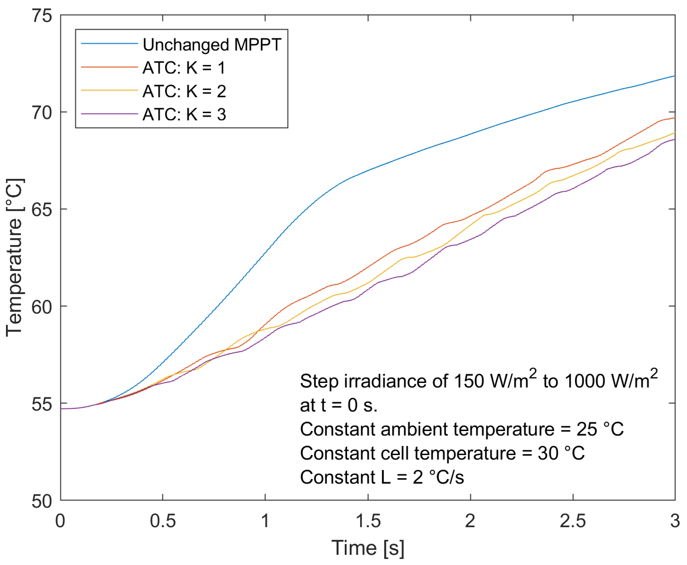
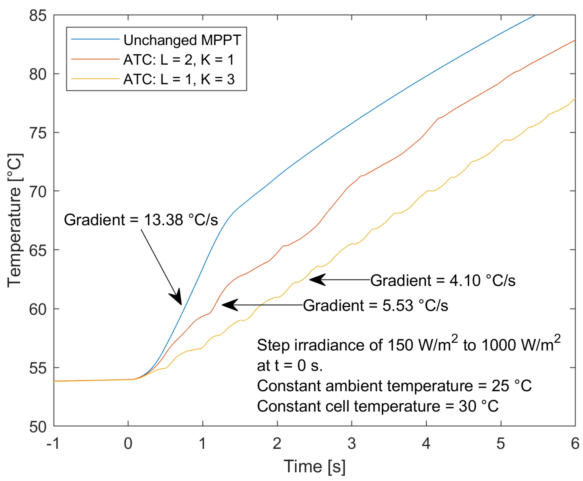
Figure 13 shows the reduction in temperature rise when a step irradiance is applied. The temperature rise rate seen is larger than the set limit. This is due to the increase in irradiance, which causes a rise in power generation.

Figure 12 shows the algorithm results with consideration of different K values. The rate limit L is the dominant parameter for the rate of junction temperature increase where the effect of K is not as pronounced.

Figure 13 demonstrates the effectiveness of the proposed algorithm, whereby the rate of junction temperature increase is decreased from 13.4 ${}^{°}$C/s using an unchanged MPPT algorithm to 4.1 ${}^{°}$C/s. As expected, decreasing the rate limit L and increasing the constant parameter K correspond to making more common and dramatic changes to the duty cycle, shown by the decreasing rate of junction temperature increase. The different parameters show that tuning is capable of adjusting the rate, which is related to the trade-off between MPPT speed (and, therefore, energy generation) and transistor damage accumulated. The slight variation in the temperature is a consequence of having the limit term L, such that the algorithm is cycling between on and off as the temperature rise fluctuates around the limit value. A lower limit is seen to cause a larger amount of variations as it is more frequently switching between active and inactive states.

The average rate of junction temperature increase is higher than the set limit L for both cases in Figure 13. With a dramatic increase in irradiance such as the one used from 150 W/m${}^2$ to 1000 W/m${}^2$, the power flow will correspondingly increase dramatically. This means that, in effect, the temperature rise due to this increased power flow cannot be compensated or slowed sufficiently by the algorithm. As a result, the temperature rise rate will exceed the set limit. With smaller or slower increases in irradiance, the algorithm is capable of achieving the set rate limit.

5. Simulation and Network Training

With the infeasibility of calculating lifetime consumption in an experimental setup, as shown in the current literature [8,10,18,21], a MATLAB/Simulink approach was taken. The electrothermal model was implemented into Simulink using the specialized power systems library.

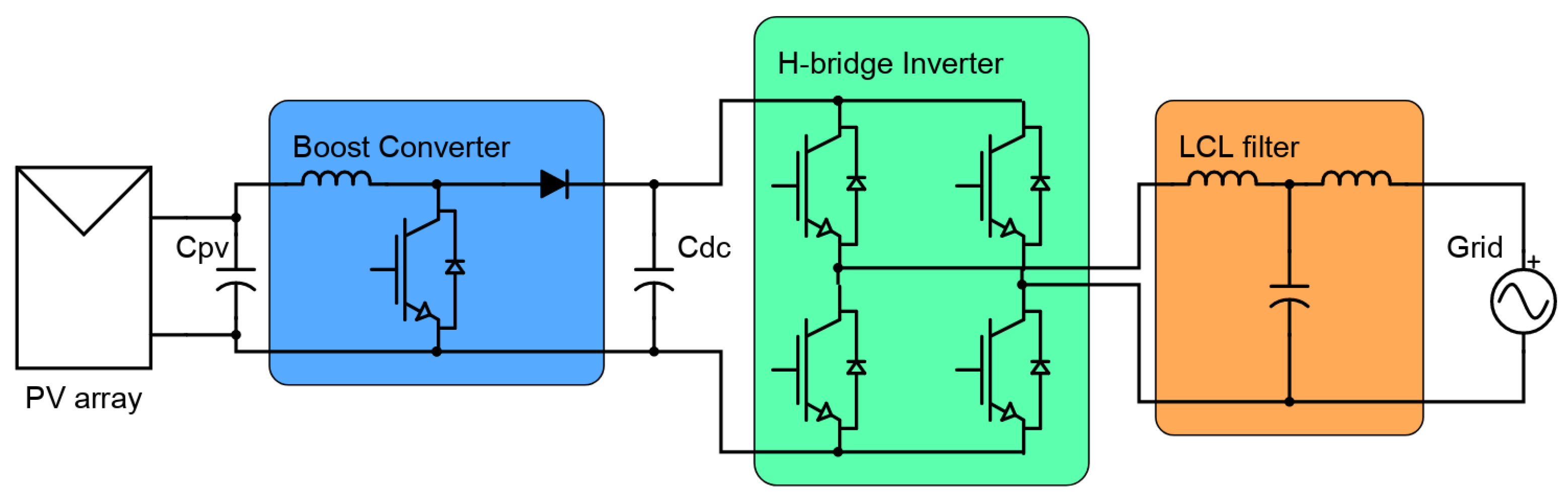
The electrical design parameters and components of the studied system are shown in

Table 2. System electrical design parameters and components.

Quantity	Value
Rated power	10 kW
RMS grid voltage	240 V
Grid frequency	60 Hz
DC link voltage	450 V
DC link capacitor	2100 $\mathsf{\mu }$F
PV capacitor	2100 $\mathsf{\mu }$F
Inverter switching frequency	7.5 kHz
Boost converter
Switching frequency	7.5 kHz
Inductor value	1.5 mH
LCL filter
Inverter side inductor	8 mH
Capacitor	5 $\mathsf{\mu }$F
Grid side inductor	4 mH
Datasheet components
IGBTs	Infineon IKW40N60H3
PV panels	Trina Solar Vertex DE19 555W

. The PV array is connected with 2 parallel strings with 9 series-connected panels on each string, with an array total open circuit voltage, $V_{oc}$, of 342.90 V and short circuit current, $I_{sc}$, of 37.12 A, assuming identical panels.

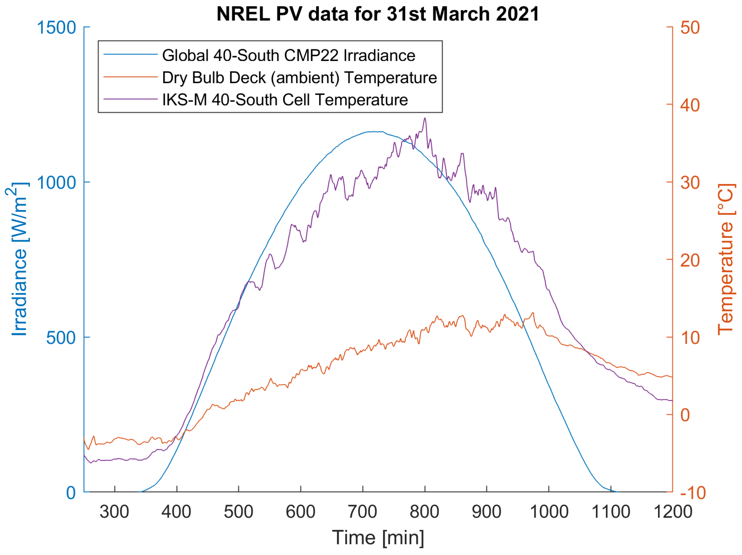
The data used in this study are from the Baseline Measurement System dataset from the National Renewable Energy Laboratory’s Solar Radiation Research Laboratory (SRRL) in Golden, CO, USA [42]. For measuring total solar irradiance, a CMP22 pyranometer inclined at 40-South is employed. The ambient temperature is taken from the instrument deck. The cell temperature uses data from IKS-M 40-South, part of the SRRL PV Resource study, located on the same site. While temperature data are available for the CMP22 pyranometer, it is believed that using PV cell temperatures would be a more realistic temperature representation for the electrical model in this study. Figure 14 shows an example of the raw environmental data source from one particular day, with the cell temperature more closely correlated to irradiance than ambient temperature.

Starting 1 January 2021, 365 days of data are used. The irradiance data below 1 W/m${}^2$ were removed as these do not contribute significantly to energy generation and provide very minimal lifetime consumption while greatly increasing the amount of time required for simulations.

The training data were carefully chosen to encompass a diverse set of conditions related to irradiance and temperature at this specific location. Meanwhile, the testing data were randomly selected. The training dataset consisted of six days, amounting to 3726 data points, while the testing dataset included seven days, comprising a total of 4762 data points.

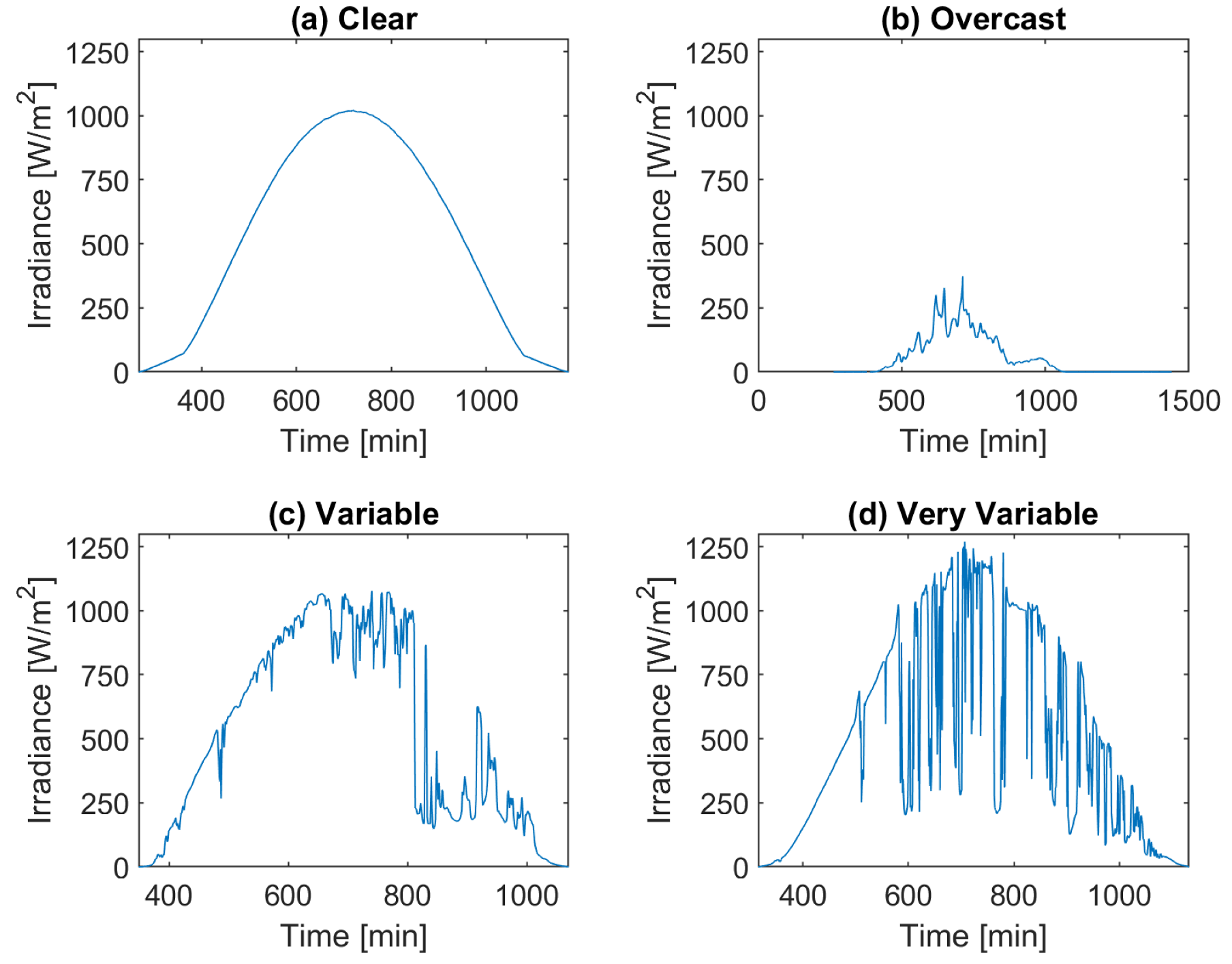
Figure 15 illustrates examples from four subsets of environmental conditions: clear, overcast, variable and very variable. The data were sorted manually, taking into account peak irradiance and irradiance changes.

Table 3. Number of days in each subset.

Day Subset	Number of Days
Clear	108
Overcast	30
Variable	136
Very variable	91

shows the number of days in each subset. By applying the trained neural networks to each subset, it can be seen how the proposed algorithm performs under different conditions.

For the ANN, three hidden layers were used, with each bracketed value in

Table 4. Neural network parameters.

Network Predictor	Hidden Layer Structure
LC	[10, 30, 1]
EG	[5, 20, 4]

denoting layer size. The layer structure can be seen in Figure 6 and Figure 7. It was found that the hidden layer structure was not critical for accuracy provided the layers were sufficiently large. For example, the accuracy of a network with a structure of [10, 30, 1] had very little difference from that of [5, 40, 1]. The hidden layer activation functions were tanh for both LC and EG networks. The larger hidden layer sizes increase training computation time. No regularization was used. Network inputs were standardized. Network target values were scaled to a range of 0 to 1.

Due to the statistical nature of network training, it was repeated five times in total. The training was repeated five times to account for the statistical variability in neural network training, as each run can yield slightly different results due to random initialization and optimization processes. The optimal number of repetitions depends on factors such as model complexity, dataset size, and available computational resources. Generally, conducting multiple repetitions (e.g., five) provides a more robust estimate of the network’s performance. However, there are diminishing returns with increasing repetitions, and the choice of the optimal number should strike a balance between statistical confidence and practical considerations. Each trained network was then applied to the testing data. The best performing network on the testing data was selected and applied to the long-term data. The network performance was measured with the error percentage of total LC or EG to the simulated values, as can be seen in Equation (6). The networks chosen using mean squared error (MSE), the performance metric used in fitrnet, proved to be less accurate, particularly in LC values. Using error percentages also gives a better understanding of accuracy, whereas MSE requires further context or comparison to understand.

$$\mathrm{Error}\% =100·|1-\frac{\sum \mathrm{Predicted}\mathrm{LC}\mathrm{or}\mathrm{EG}}{\sum \mathrm{Simulated}\mathrm{LC}\mathrm{or}\mathrm{EG}}|$$

(6)

Two sets of ATC parameters were tested to show the trade-off between energy generation and lifetime improvement. The context for the relevant parameters is found in Section 5. The algorithms using the parameters from

Table 5. ATC parameters used.

ATC No.	L	K
1	2	1
2	1	3

are referred to as ATC no. 1 and 2. The $\Delta D$ value was a constant of $3\times {10}^{-7}$ for the P&O and ATC algorithm. The reduction in junction temperature gradient for both of these sets of parameters can be seen in Figure 13.

6. Results and Discussion

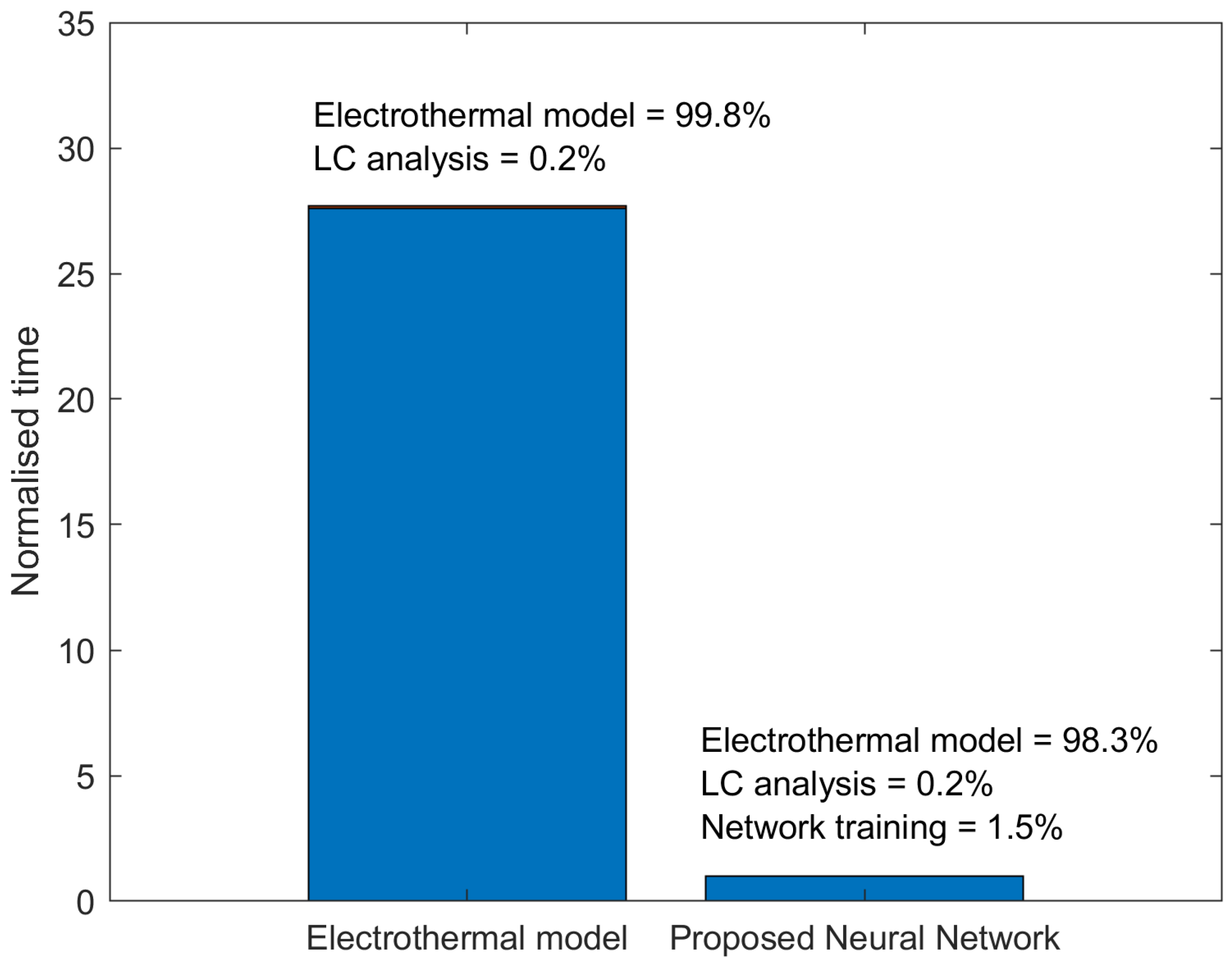
In both simulation time and total data storage space requirements, the neural network method proposed in this paper is an overwhelming improvement on traditional electrothermal models for long-term analysis. Where long-term analysis is required, using neural networks would significantly speed up development processes, meaning more effective and time-efficient designs for reliability studies can take place. The speed improvements seen in Figure 16 and

Table 6. Estimated time and storage needed for simulating 365 days of data using an electrothermal model normalized to a neural network regression approach.

Simulation Type	Total Time	Storage Requirements
Electrothermal model	27.6	28.0
Proposed Neural Network	1	1

when using the neural networks can be further improved by optimizing the amount of training and testing data. The time required for either long-term simulation or neural network training is dominated by the electrothermal model simulations, taking 99.8% and 98.3% of the total time, respectively. However, reducing the amount of training data too far results in low accuracy.

It is only economical to use neural networks as outlined when the amount of data required to predict exceeds the amount of training and testing data. Otherwise, standard electrothermal models are sufficient. Using the example of this study, with 13 days of combined training and testing the simulation, the benefits of using a neural network begins when 14 days or more are required.

Long-term data of any length could be used with no further electrothermal simulations required. However lifetime consumption values become less accurate with larger timescales as degradation becomes more prominent, and no feedback metric for degradation is applied in this paper. One year of data are used here for a balance of maintaining accurate electrothermal properties, while also ensuring a mixture of conditions, and long-term performance is still analyzed.

Due to the small sample size of electrothermal modeled days, and with training data being cherry-picked, the results in

Table 7. LC and EG percentage change using the proposed ATC algorithm from training and testing electrothermal model data relative to an unchanged P&O algorithm.

MPPT Algorithm	LC (% Change)	EG (% Change)
ATC no. 1	−1.34	−0.33
ATC no. 2	−5.42	−1.61

may not be representative of the long-term trends. Additionally, small trends may be present in the electrothermal results, but in such limited quantity to appear insignificant in the results. As a result, long-term simulations show a better approximation of how it would operate if placed in the field.

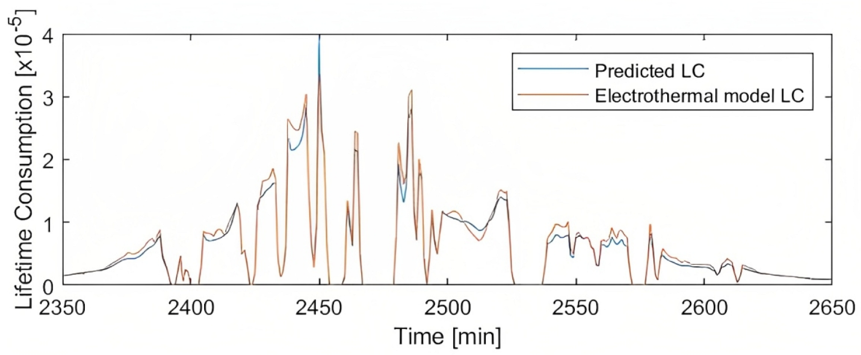
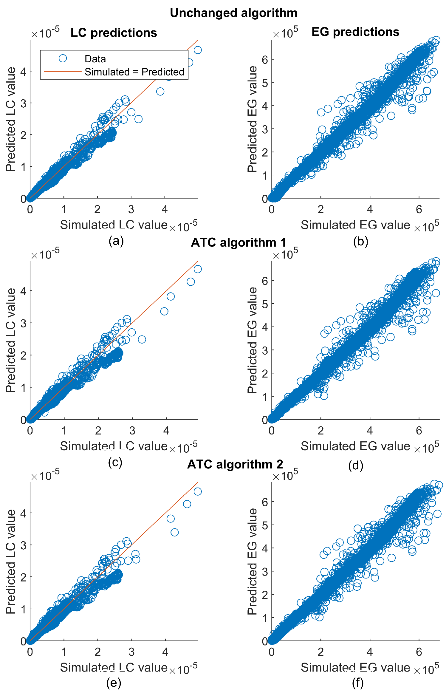
When examining the accuracy of the neural network, it can be seen that it performs to a high standard. Figure 17 shows the lifetime consumption estimations for a full day for both the electrothermal model and the neural network. Figure 18 shows a scatter plot of the accuracy in network predictions on the testing set for all the available data. Ideally, the predictions and simulated results would be equal, therefore, producing a linear line of slope 1. As a result, deviation from the line demonstrates errors in the predictions. The plots clearly show that the neural networks remain reasonably accurate for high lifetime consumption value predictions, even with relatively few observations. There is an increasing amount of error in LC with the increasing value, possibly due to the decreasing availability of training data for higher values. Furthermore, 72% of the simulated LC values were below $0.1\times {10}^{-5}$. EG can be seen as relatively easier to predict, with lower deviations from the ideal case. Energy generation, majoritively a function of irradiance, naturally sweeps through almost all the values between 0 W/m${}^2$ and its peak twice per day, whereas lifetime consumption, a more complex function, does not present such an easy target for training. This means that selecting accurate training data in the aim of optimizing lifetime consumption training is non-trivial and is the limiting step in overall network accuracy. This is demonstrated numerically in

Table 8. Neural network regression accuracy in predicted values against the testing data.

MPPT Algorithm	Total Testing Error (%)		Correlation (%)
	LC	EG	LC	EG
Unchanged	2.57	0.15	99.2	99.6
ATC no. 1	3.39	0.51	98.8	99.5
ATC no. 2	3.07	0.52	98.8	99.5

, where the percentage LC error is up to six times higher than for EG.

In this study, the proposed neural network was used to predict LC and EG values, with the later intention of comparing the outputs to determine the effectiveness of the proposed ATC algorithm. However, the neural network demonstrated in this paper can be easily applied to any PV system. While network training still requires an electrothermal model, it has demonstrated effectiveness in predicting values for the long-term data. Neural network predictions modeling PV systems could be used in the design and analysis stage of novel PV system designs or integration. Neural networks have already been applied to energy forecasting; however, this paper also demonstrates the use for reliability studies [43,44,45].

The results shown in

Table 9. LC and EG percentage change when using the proposed ATC algorithm when applied to a year-long dataset relative to an unchanged P&O algorithm.

MPPT Algorithm	LC (% Change)	EG (% Change)
ATC no. 1	−1.08	−0.47
ATC no. 2	−3.26	−0.98

agree with the electrothermal simulations with a demonstrated trade-off between lifetime improvement and energy generation, as shown by ATC no. 1 and 2. The parameters for the algorithm described in Section 4 can be tuned for any compromise level between lifetime improvement and energy generation. There is a small decrease in LC change compared to Table 7. This could be explained by the cherry-picked data and small sample size, as noted previously. However, these could also be explained by network inaccuracy.

While reducing the energy generation seems counter intuitive, it is offset by increasing the lifetime of the system. The aim is to minimize the total cost of the system over its entire life; therefore, the trade-off between lifetime improvement and energy generation demonstrated by the proposed algorithm can be used to find the optimal point. As mentioned, PV is set to play a large role in the decarbonization of energy generation globally, and reducing the levelized cost of energy is key to this role.

The results of [20] showed a significant decrease in device lifetime models when a model for degradation feedback was included. Therefore, it is suspected that if these feedback models were applied to the ATC algorithm shown in this paper, the lifetime improvements over an unchanged algorithm would increase above those shown in this section.

Table 10. LC and percentage change when using the proposed ATC algorithm split by day type relative to an unchanged P&O algorithm.

MPPT Algorithm	LC (% Change)	EG (% Change)
Clear
ATC no. 1	−1.14	−0.23
ATC no. 2	−1.59	−0.55
Overcast
ATC no. 1	327.84	−7.13
ATC no. 2	−73.503	−5.77
Variable
ATC no. 1	−2.08	−0.30
ATC no. 2	−4.26	−0.90
Very variable
ATC no. 1	−1.09	−0.46
ATC no. 2	−4.43	−1.35

presents the data split by environmental conditions. The high variation in LC seen for overcast days is due to the lower absolute LC values. This causes network inaccuracies to become more prevalent on a percentage basis. Very variable days result in 39.2 times more lifetime consumed on average than overcast days; therefore, in absolute value, improvements to overcast days are not critical. Clear days, on average, have 4.9 times greater peak solar hours compared to overcast days, where peak solar hours are equivalent to hours at an irradiance of 1000 W/m${}^2$. This means, on average, there is approximately 4.9 times more energy generation over a clear day than overcast. Additionally, overcast days occur at a rate 3.6 times less frequently than clear days. Consequently, sub-par energy performance on overcast days does not significantly reduce total energy generation over a year.

Table 11. Comparison of LC and EG percentage change when using the proposed ATC algorithm when applied to a year long dataset relative to an unchanged P&O algorithm.

Paper	LC (%)	EG (%)	Analysis Duration
This paper	−3.3	−1.0	365 days
Andresen et al. [6]	−13.0	−3.7	10 min
Tapia et al. [18]	−4.6	−0.02	4 days

shows the advantage of this paper over the existing literature. The LC and EG percentage changes for this paper are approximately a factor of four less than those of [6], suggesting similar results could be achieved with careful consideration of the algorithm parameters. With a much longer analysis duration, more confidence can be given to the results, and a better understanding of the benefits over real-world implementation can be ascertained. As mentioned previously, there are dramatic differences in the conditions over a year. Consequently, to suggest that the results seen in [6] could hold throughout a year of mixed conditions would be incorrect. Using real irradiance data means that the results in this paper represent a more reality-true picture of the algorithm benefits [18] presents favorable improvements at face value. However, with an accuracy of 95.3% for lifetime consumption compared to the above 97% accuracy in this paper, this difference in results between papers may be statistically insignificant. Additionally, while four days total of testing data are an improvement over [6], with only one day from each cloud cover category, it can be said to not be demonstrative of long-term trends, as some aspects of the small dataset may be amplifying results. Consequently, there is low confidence in the results until long-term data are used.

The techniques and results in this paper are intended for the improvement of the design for reliability studies by making economical the use of long-term datasets, allowing more reliable study insights. Compared with the existing literature, in which datasets are often at most a small number of days, the datasets used in this paper can be described as long-term as they total a full year.

7. Conclusions

This paper details the theory, implementation and results for a novel active thermal control MPPT algorithm utilizing neural networks for long-term analysis. The current literature uses short analysis durations and non-real irradiance data, limiting the analysis of the effectiveness under real-world conditions. In contrast, this paper implements long term analysis techniques and uses real meteorological data.

The proposed algorithm functioned as desired, reducing lifetime consumption values. A trade-off between lifetime improvements and energy generation was demonstrated. The algorithm parameters can be tuned to the designer’s specifications.

The neural networks were utilized to great effect for predicting lifetime consumption and energy generation values. Lifetime consumption was more difficult to accurately predict than energy generation. The results proved that this prediction method can be used for accurately modeling any PV system. Due to the requirement of electrothermal modeling for generating the training and testing data, the time and storage benefits of using neural networks are only present when long-term predictions are needed.

Further work could include using a higher resolution dataset, such as data sampled every second. One such dataset is available from the National Renewable Energy Laboratory. This could potentially increase neural network accuracy, as it would increase the amount of training data by a factor of 60. Additionally, it would better represent real-world conditions, which could change on a second by second basis.

The authors also envision several other promising future research directions for active thermal control MPPT algorithms utilizing neural networks in the renewable energy domain. First, efforts should focus on enhancing prediction accuracy by exploring advanced neural network architectures. Integrating real-time data into the algorithms would also enable real-world performance monitoring and dynamic adaptation, leading to improved overall efficiency and reliability. To optimize the trade-offs between lifetime improvements and energy generation, the research can investigate novel cost–benefit analysis frameworks and consider factors such as component aging, maintenance costs and environmental impact. Furthermore, expanding the application of active thermal control MPPT algorithms to other renewable sources, such as off-shore grid-connected wind farms, presents a promising avenue for research. Wind power converters face unique challenges related to harsh environmental conditions and variable wind patterns, and thus, customized approaches tailored to the specifics of wind energy systems are essential. Moreover, the research could focus on optimizing computational efficiency, reducing model complexity and exploring edge computing or hardware accelerators to enable real-time implementations of these algorithms in resource-constrained environments.