1. Introduction
Lithofacies identification is an essential tool in geologic investigation, where a rock type or class is assigned to a specific rock sample based on measured properties [
1]. The accuracy of this identification process directly affects reservoir evaluation and development plan formulation [
2,
3]. The traditional approach to lithofacies identification uses core- and thin-section analysis from cored-well matched with well-logs [
4,
5,
6]. However, the collection of core samples and thin sections is often constrained by time and cost. As such, indirect estimation is often required to identify lithofacies [
1]. Wire-line log measurements, such as gamma ray, neutron porosity, and resistivity are widely used to identify lithofacies for non-cored wells and intervals. However, the manual interpretation of wire-line log measurements constitutes a massive data analysis challenge for skilled interpreters and is therefore difficult to manage for many wire-line logs [
7]. The process often misses valuable information and results in increased cost and decreased efficiency. Additionally, the process often introduces errors and multiplicities [
8]. Therefore, a fast, accurate, and automated approach, reducing the need for experts’ involvement, would be beneficial. To address these challenges, different AI- and non-AI-based computational techniques and algorithms have long been used. These approaches include support vector machines (SVMs) [
9], k-nearest neighbors (k-NNs) [
1], fuzzy logic [
10,
11], artificial neural networks (ANNs), and machine learning [
4,
12,
13,
14]. The fundamental goal of these methods is to use quick, repetitive calculations with complex equations to find the spatial and mathematical correlations between wire-line log data and lithofacies.
Artificial neural networks (ANN) and machine learning (ML) techniques aid researchers in extracting valuable insights from datasets. These techniques are particularly effective in handling non-linearities inherent in wire-line log data [
15,
16]. ML, leveraging data-driven decision-making, efficiently captures information from wire-line logs without manual rule creation. With increasing computational power, these techniques have become popular for identifying lithofacies. Machine learning accuracies hinge on training phases, categorized into supervised, semi-supervised, and unsupervised techniques [
4,
17]. In supervised learning, where models are trained with annotated data, challenges arise due to limited annotated data for lithofacies identification [
18,
19]. Training with a lower percentage of annotated data introduces random noise and hampers generalization [
20]. Semi-supervised learning, utilizing both annotated and non-annotated data, offers improved accuracy when annotated data are scarce [
21,
22]. Unsupervised machine learning models, unlike their counterparts, require no annotated data for training, autonomously extracting hidden patterns [
23,
24]. Popular unsupervised techniques, such as deep convolutional autoencoders (DCAEs), k-means, and t-distributed stochastic neighbors (t-SNE), have gained prominence in lithofacies identification and broader geological investigations [
25,
26].
Cluster analysis, widely employed in data analysis and statistics, finds significant application in lithofacies identification due to its efficacy without annotated data [
8,
27,
28,
29]. Data clustering techniques facilitate the identification of clusters within wire-line log data, with the subsequent assignment to specific rock samples based on representative log signatures or core data from core- and thin-section observations, avoiding the need to analyze every detail of each well. Clustering can be executed with or without machine learning techniques. Popular non-machine learning clustering algorithms include k-means [
30], hierarchical clustering [
31], and density-based clustering (e.g., DBSCAN) [
32]. In contrast, self-organizing maps (SOM), a widely used unsupervised machine-learning-based algorithm, stands out for its advantages in lithofacies identification [
15,
33].
Lithofacies identification through data clustering is crucial for geological investigation, especially when dealing with the absence of annotated data. However, challenges arise as algorithms like k-means, hierarchical clustering, and SOM necessitate a predefined number of clusters, requiring prior knowledge about the dataset. This imposes the need for human interpretation before applying clustering algorithms, particularly when accurate cluster numbers are vital. Density-based clustering, while capable of identifying clusters, often struggles with noise and scalability issues [
34]. An ideal data clustering algorithm for lithofacies identification should not only derive cluster numbers from data distribution but also be efficient, scalable, and work with large-scale high-dimensional data without dimension reduction [
5]. The piecemeal clustering algorithm [
35], an unsupervised learning-based method that adapts the SOM training technique and integrates it with agglomerative hierarchical and density-based clustering, is employed to addressing these needs. The algorithm utilizes Euclidean distance and cosine similarity, considering all properties of each input data sample. Crucially, it automatically identifies the number of lithofacies and maps data points to their best-matched lithofacies, eliminating the need for a priori knowledge.
This study explores lithofacies identification from wire-line logs using the piecemeal clustering algorithm, focusing on two key research questions: (a) Can the piecemeal clustering algorithm identify lithofacies without prior knowledge of their number? and (b) Does this algorithm produce comparable results to other data clustering methods, as well as supervised and semi-supervised machine learning techniques? To find the answers of these questions, the piecemeal clustering algorithm was applied to wire-line data from ten wells in the Hugoton and Panoma fields in southwest Kansas and northwest Oklahoma. These wells were part of an earlier investigation into the geological and reservoir properties of the Anadarko Basin, resulting in a detailed stratigraphic framework [
36] and insights into the basin’s depositional history and hydrocarbon implications [
37]. Nine lithofacies were previously identified in the dataset [
36], consisting of five wire-line logs recorded at half-foot depth intervals, including gamma ray (
GR), resistivity (
ILD_log10), photoelectric effect (
PE), neutron-density porosity difference (
DeltaPHI), and average neutron-density porosity (
PHIND). Additional geologic variables augment the dataset, with a comprehensive description provided in
Section 3. The dataset was made publicly available through an SEG competition held in 2016 [
19,
38]. Gaussian naïve Bayes (GNB) [
39], support vector machines (SVM) [
40], XGBoost [
38], level propagation (LP) [
4,
22], and self-trained LP [
4,
41] are some of the methods previously applied on the dataset to determine the lithofacies, and showed promising results. The result from piecemeal clustering is compared to those results in this study, besides comparing it with other data clustering methods from the literature.
The outline of this paper is as follows. The paper begins by outlining the piecemeal clustering algorithm. It then introduces the wire-line log dataset and frames lithofacies identification as a clustering problem. Then, the results of our study are provided and compared with other algorithms mentioned above. Finally, the implications of the results are discussed followed by conclusion.
2. Methodology
Data clustering systematically arranges data into distinct groups. The distinct groups contain data that have a high degree of similarity among the elements chosen to describe them. Elements are discernibly different between groups [
34]. Mathematically interpreting data clusters in the context of lithofacies identification from wire-line logs requires the mathematical definition of the terms
data point and
cluster, along with other relevant concepts such as
distance,
representative cluster model, and
membership mapping.
A
data point, in this context, represents the physical properties at a certain depth in the well. Each data point is considered to be an
n-dimensional vector
in hyperspace as represented in Equation (
1), where each of the scalar components
of the vector represents one of the physical properties measured by wire-line logs, such as gamma-ray (
GR), resistivity (
ILD_log10), and average neutron-density porosity (
PHIND).
The likelihood is high that two vectors are similar if the depths from which the vectors are drawn are part of the same lithofacies. One of the ways to determine whether two vectors are similar is to calculate the
distance between them. The distance between two vectors can be measured in a variety of ways.
Euclidean distance,
, is one of the most common methods of measuring the distance between two
n-dimensional vectors
and
, where the differences between respective components are used as in Equation (
2):
where
Euclidean distance measures the distance solely based on the magnitudes of the differences between the corresponding vector components, and discounts the vectors’ similarity in their hyper-planes.
Cosine similarity,
, on the other hand, uses the hyperplane on which two vectors lie to define the similarity between two vectors as shown in Equation (
3). Here, the similarity can be used as a proxy for the distance between two vectors: the higher the similarity, the lower the distance, and vice versa.
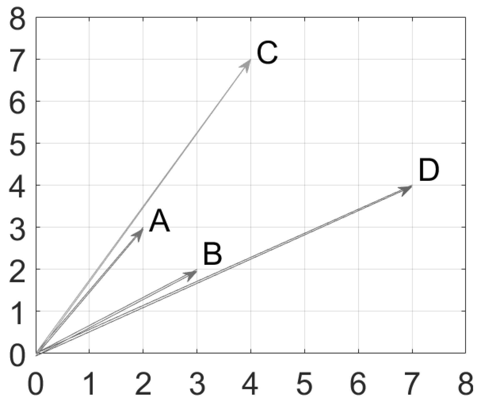
Figure 1 shows an example of how the two distance measurements, Euclidean distance and cosine similarity, vary in two-dimensional Euclidean space. The vector
is closer to
than to vector
if the distances are measured using Euclidean distance. Alternatively, vector
is closer to
than to vector
if the cosine similarity is used instead, since
and
have a very small angular difference compared to the angle between
and
.
When using data clustering to identify lithofacies from wire-line logs, one or more clusters may be part of the same lithofacies. Each cluster is often represented using its respective cluster center, a representative model of the cluster defined by a vector with the same number of components as the data point. The data points closest to the cluster center, based on a defined distance measurement, are considered members of the cluster represented by the cluster center.
2.1. Self-Organizing Maps (SOM)
The self-organizing maps (SOM) clustering algorithm starts with an initial user-defined number of clusters with their respective cluster models, which are often randomly selected [
42]. The unsupervised learning iterations then move the cluster models towards the high-density regions of the data points closest to them using an iterative learning algorithm. The learning algorithm takes a cluster model and one data point at a time to measure the degree of adjustment using two factors: Euclidean
distance between the pair and the
learning rate. The learning rate is initially selected by the user and exponentially decreases with each iteration. At the same time, the learning algorithm uses only those data points within a certain
radius from the cluster models in terms of the distance. The initial radius value typically commences at half of the maximum Euclidean distance between any two data points in the dataset, gradually and exponentially decreasing over iterations. At the end of the iterations, each of the data points is mapped to the cluster model it is closest to.
2.2. Piecemeal Clustering
The key disadvantage of self-organizing maps is that the maximum number of clusters it can produce is limited to be equal to the initially selected number of cluster models. The result is also heavily dependent on how the initial models are selected. Piecemeal clustering solves this problem using a three-phase approach. The first phase, pre-clustering, selects the initial set of cluster models and their representative models (cluster centers). This phase initially produces a larger number of clusters using the agglomerative hierarchical clustering technique. Agglomerative clustering uses the concept that each data point is itself initially a cluster and therefore by extension, also a cluster center, which can be used to model its cluster. The closest clusters are iteratively merged to form new clusters with new cluster centers defined by the centroids of the member data points of newly merged clusters.
Piecemeal clustering uniquely combines Euclidean distance and cosine similarity to measure the distance between two data points or between a data point and its corresponding cluster center. Therefore, both the magnitudes of the different vector components and their alignment in the hyperplane are accounted for in the measurement. This type of measurement is a novel feature of this clustering algorithm.
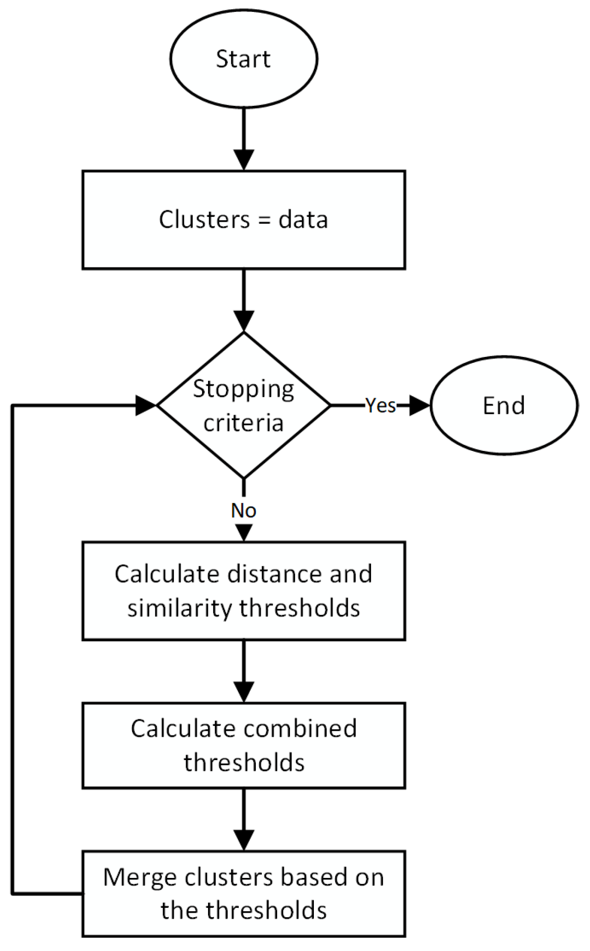
Figure 2 shows the pre-clustering flowchart and the description of the algorithm for this phase which are from Hasan et al. [
35].
The pre-clustering phase uses a parameter T, called the cutoff threshold, to define when the phase will stop. The users can choose a value of T as an input to the algorithm, based on their domain knowledge about the dataset, to define the minimum natural or expected variation in the members that a cluster may have. The input parameter T is measured in terms of the percentage of the maximum Euclidean distance between any two data points in the dataset. It is recommended to use a lower value of T when presented with a range of natural or expected intra-cluster dissimilarities or if an actual measurement is difficult to determine. The value of the cutoff threshold is only used by the algorithm to stop the pre-clustering phase and not to reach the globally optimal clustering. At best, this phase can in general only reach a locally optimum clustering. A lower value of T ensures that the globally optimal clustering is not excluded from consideration in the later phases of the algorithm. In the later phases, the nearby small clusters will be merged to form the final set of clusters. Therefore, the algorithm is robust to small changes in the value of T.
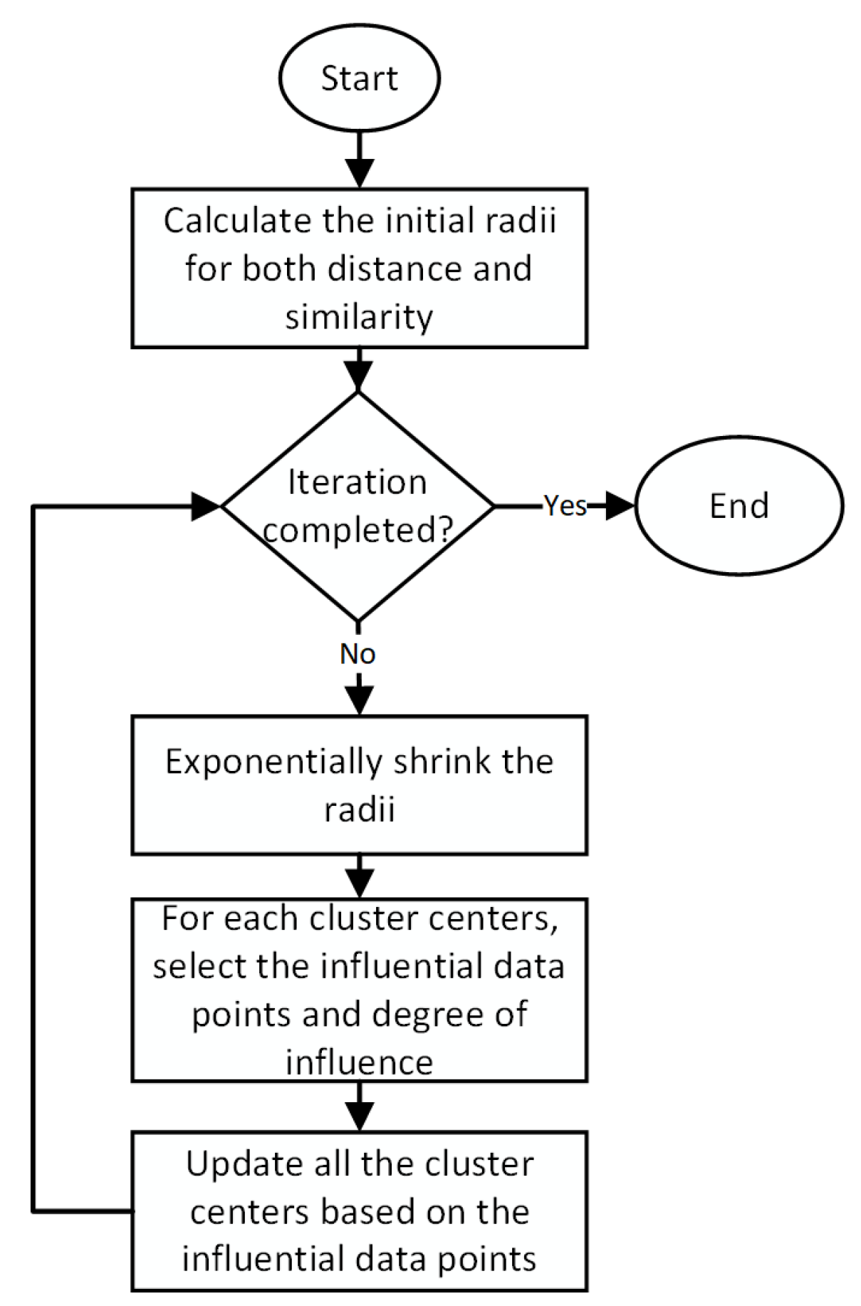
In the second phase,
training, the algorithm uses a very similar approach to self-organizing maps (SOM) to move the cluster centers towards the high-density data regions closest to them. Unlike SOM, the cluster centers are already defined in the pre-clustering phase based on the local density of the data points, making the training phase more accurate and effective. The flowchart for this phase is shown in
Figure 3 and the algorithm details are given in Hasan et al. [
35].
The training phase can be adjusted by selecting the learning rate and the stopping
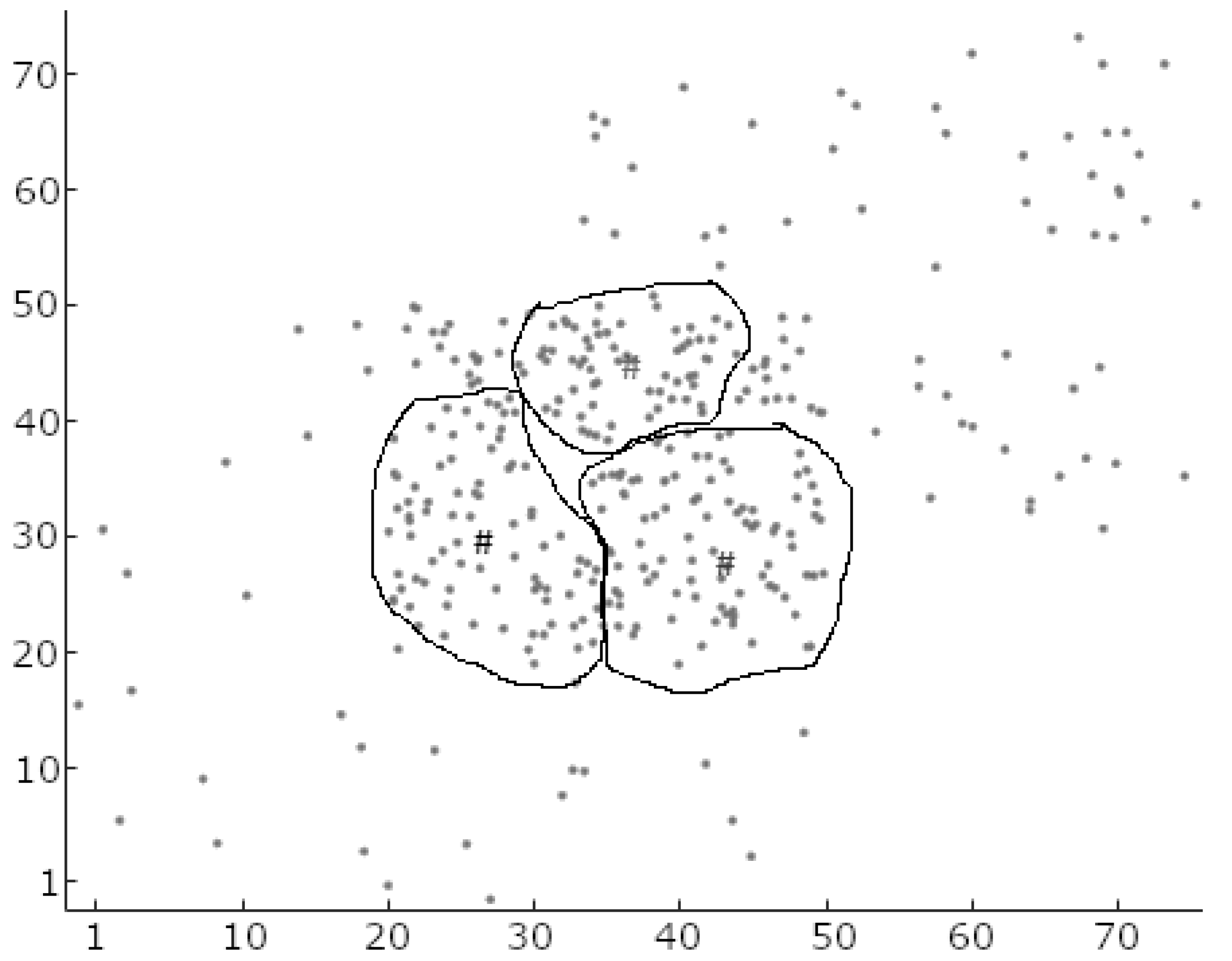
iteration number. These two parameters carry the same meanings and purposes as for the self-organizing maps (SOM) algorithm, and a similar approach to that used in SOM can be used to find the correct values. The piecemeal algorithm suggests a trial-and-error approach to select values where the sum of the distances from the data points to their respective cluster centers is the lowest for the entire dataset. The learning algorithm of this phase disregards the perceived membership of data points (local data density) found in the pre-clustering phase and considers the global data density to adjust the positions of the cluster centers. Therefore, at the end of this phase, the clusters are different in terms of their shapes and sizes. If there is more than one cluster center found within a dense set of data points, as shown in
Figure 4, the training algorithm positions the cluster centers in such a way that the next phase, post-processing, merges them together to form a single cluster. Further detail of the algorithm and mathematical formulation can be found in Hasan et al. [
35].
3. The Dataset
The Hugoton and Panoma field dataset has been used to investigate the geological and reservoir properties of the Anadarko Basin, formed during the late Paleozoic and early Mesozoic eras, which contains sedimentary rocks deposited in various environments. Dubois et al. [
36] developed a detailed stratigraphic framework for the Basin using this dataset, allowing for the identification of potential reservoirs and the reconstruction of depositional environments. Avseth et al. [
37] used the dataset to investigate the depositional history of the basin and its implications for hydrocarbon exploration. Hall and Hall [
38] examined the reservoir properties of the rocks in the region, such as porosity and permeability, while Hall [
19] developed a depositional model for the Hugoton and Panoma fields. Dunham et al. [
4] investigated the depositional history and stratigraphy of the region using the same dataset, demonstrating the value of the Hugoton and Panoma dataset for understanding the geology and hydrocarbon potential of the Anadarko Basin.
The wire-line log data in this dataset were collected from ten wells from the Hugoton and Panoma fields in southwest Kansas and northwest Oklahoma, respectively. The dataset includes wire-line log data and core samples recorded at half-foot depth increments for 4137 total data points. Dubois et al. [
36] determined that there are nine lithofacies or classes in this dataset. The first three lithofacies are non-marine, while the remaining six are marine lithofacies. Each well in the dataset is accompanied by five wire-line logs, including gamma ray (
GR), resistivity (
ILD_log10), photoelectric effect (
PE), neutron-density porosity difference (
DeltaPHI), and average neutron-density porosity (
PHIND). Additionally, there are two geologic variables provided for each well: the non-marine/marine (
NM_M) indicator and relative formation position (
RELPOS). The descriptions of these lithofacies and their depositional environments are provided in
Table 1.
The
NM_M indicator in the dataset is used to separate the non-marine and marine lithofacies, indicating that they may exist on separate manifolds. The relative formation position variable provides information on the vertical position of the lithofacies within the well [
36]. The lithofacies identified in the dataset reflect a diverse range of depositional environments, including shallow marine, fluvial, deltaic, and aeolian. The lithofacies include sandstone, shale, siltstone, and limestone [
36].
The wire-line logs in the dataset provide information on the formation properties, such as mineral content, porosity, density, and any fluid saturations (water, oil, and gas). The Gamma ray log measures the natural gamma radiation emitted by the rocks, which can be used to identify different lithologies. The resistivity log measures the electrical resistance of the rocks, which can provide information on the fluid content and mineralogy. The photoelectric effect log measures the absorption of gamma rays by the rocks, which can be used to estimate the mineral composition [
45,
46]. The neutron-density porosity difference log measures the difference between the neutron and density porosities, which can be used to estimate the porosity and lithology. Finally, the average neutron-density porosity log measures the average porosity of the rocks.
To interpret the subsurface geology and evaluate reservoir quality using the traditional method, it is important to understand the
GR and
DeltaPHI values in various lithofacies and depositional environments. Geologists can better comprehend the characteristics of rock formations and make more precise predictions about their suitability for hydrocarbon exploration and production by evaluating wire-line logs and other data. The higher maximum value of the
GR logs for marine data points suggests that marine sedimentary sequences are more likely to contain highly radioactive minerals, such as clay minerals, organic matter, and glauconite [
47]. The higher levels of inherent radioactivity of the material can contribute to increased GR measurements. On the other hand, the lower means and higher standard deviations of the
GR values for the marine data points may suggest that the lithology and depositional environments of marine sedimentary sequences are more varied, resulting in more variable
GR readings [
48,
49]. As a result of more uniform sedimentation and depositional processes, non-marine settings may have lower overall maximum gamma-ray values but more consistent
GR measurements. The similar ranges of values for
DeltaPHI indicate that porosity fluctuations in marine and non-marine sedimentary sequences may be comparable. The porosity values may be more variable in marine environments, as indicated by the discrepancies in mean and standard deviation between marine and non-marine data points. This may be because the lithology and depositional histories of marine sedimentary sequences might be more complex, resulting in more varied porosity properties [
50]. On the other hand, non-marine settings might have more homogeneous sedimentation and depositional circumstances, which would lead to more consistent porosity characteristics [
51].
4. Results
The input for the piecemeal clustering algorithm groups wire-line logs at the same well depth as a single data vector. The value for PE was missing for some depths; therefore, all logs from those depths were eliminated from the dataset. Statistical analysis was then performed on each of the wire-line logs. The analysis was initially performed for all of the depths and subsequently for data based on splitting the logs into two groups using the
values: non-marine and marine.
Table 2 summarizes the results. This statistical analysis was used to determine how piecemeal clustering can be applied to lithofacies identification on this dataset.
A significant difference in the distribution between non-marine and marine data points is shown in
Table 2.
GR has a higher maximum value for marine data points than non-marine points, while marine data points have lower mean values with higher standard deviations. Meanwhile,
DeltaPHI values are spread over a similar range, and have different means and standard deviations.
As a result of this difference in the data distributions of the datasets, the piecemeal clustering algorithm was applied separately to the wire-line logs from non-marine and marine depositions. Before applying the algorithm to the datasets, each of the logs was normalized to values between 0 and 1. This prevents Piecemeal Clustering from biasing one particular log based on its reading magnitude.
The cutoff threshold,
T, for marine data points was set to 0.045 (4.5%). The number of training iterations was set to 40, and the learning rate was set to
. The parameters were set by following the guidelines provided in the piecemeal clustering algorithm as described in [
35]. The
indicator and relative position (
RELPOS) were excluded from this analysis since these are derived from the formation tops information and constrained geology. Principal component analysis (PCA) with centered and variance-based variable weights was applied before passing the data to the algorithm. The degree of separation of the signature was very narrow for marine signatures. PCA helps spread out the data [
52]. The clustering produced six clusters.
The non-marine lithofacies are well separated, and consequently, it was easier to perform clustering on these data. A much higher value for T, 0.24 (24%), was used with ten iterations and a learning rate close to for the clustering. Piecemeal clustering produced three clusters.
To understand the accuracy of each of the predicted clusters by piecemeal clustering, each cluster representing a lithofacies was labeled using its dominating members. This was achieved by cross-referencing the members of each cluster with their respective known labeling found in the dataset. For example, the first predicted cluster contained a total of 636 members. Three-hundred and nine (309) members were labeled as non-marine sandstone (SS), 168 were labeled as non-marine coarse siltstone (CSiS), and 159 were labeled as non-marine fine siltstone (FSiS) in the known results. Therefore, SS was considered to be the dominating lithofacies; and the cluster was labeled with SS. This procedure was performed for all nine clusters.
To understand the mapping accuracy of the algorithm, two types of accuracy calculations were considered: with and without adjacency facies. All the data points that were dominating cluster members in their respective clusters were considered to be correctly mapped when calculating the accuracy without considering the adjacent facies. When calculating the accuracy with the consideration of adjacent facies, the cluster members that were not part of the dominating lithofacies but part of the adjacent facies, as found in
Table 1, were also included as correctly mapped data points. For example, in the first predicted cluster mentioned above, only 309 data points were considered to have been correctly mapped when calculating the accuracy without considering adjacent facies. In contrast, when calculating the accuracy by considering the adjacent facies, an additional 168 data points were added to the set of correctly mapped data points (total 477), which were found to be CSiS-adjacent to SS. In this case, the clustering algorithm accurately mapped 45.20% of the data points when not considering adjacent facies and had an accuracy of 81.90% when considering adjacent facies.
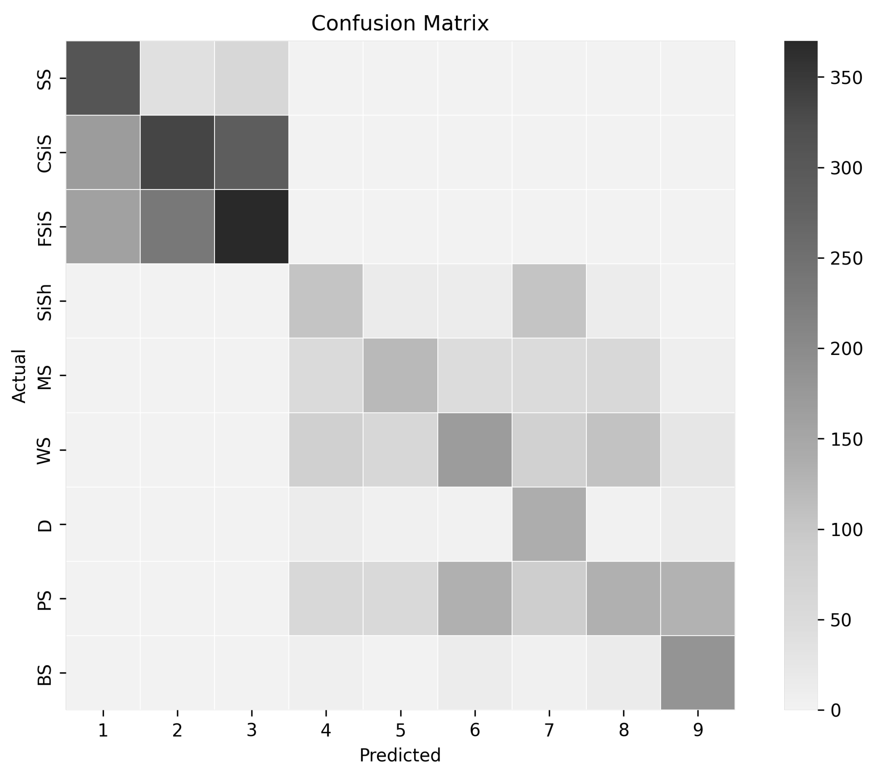
The number of elements from each lithofacies formed within a predicted cluster corresponding to a given true clusters is shown in a confusion matrix in
Figure 5. Each column represents one predicted cluster, while each row represents the number of cluster members from the known lithofacies found in each predicted cluster. For example, the aforementioned cluster is presented in column 1 in the confusion matrix. The numbers of mapped data points in each cluster are represented using gray shades, with higher numbers presented by darker gray, and lower numbers represented by lighter gray. One predicted cluster was found for each of the nine lithofacies. Therefore, the clustering algorithm accurately predicted the number of lithofacies from the dataset without using any labeled data.
Using the confusion matrix, it was also investigated whether the clustering algorithm favors isolating specific facies solely based on the wire-line log signature. In other words, how good is the algorithm at grouping the signatures from the same facies into a single cluster. The extent to which the algorithm able to accurately determine the mapping of each log signature to each of the respective facies was calculated, with and without considering the adjacent facies. The numerical result is shown in
Table 3. The confusion matrix demonstrates that the clustering performed reasonably well for some facies types but performed poorly on others. For instance, with only a few misclassifications, piecemeal clustering was successful in identifying dolomite (D) and phylloid-algal bafflestone (BS). This can be seen in the confusion matrix for rows D and BS—they are filled with lower-intensity gray for off-diagonal elements. On the other hand, for packstone–grainstone (PS) and Wackestone (WS), a large number of false positives was generated, which can also be seen in the confusion matrix, where corresponding rows have darker off-diagonal elements. A further detailed discussion of the accuracy and effectiveness of this approach is included in
Section 5.
It is important to understand how the clustering algorithm performs for each well.
Table 4 shows the name of all the wells with the breakdown of the prediction results. The names and the details of each well are found in the dataset [
19,
38].
Table 4 presents the quantity of wire-line logs, the number of logs of marine and non-marine types, and the corresponding predicted log for each well. The predicted mapping accuracy was calculated with and without considering adjacent facies. Predicted logs for non-marine facies are shown in the “predicted non-marine log” column, separated into predictions with and without considering adjacent facies. The same is performed for the marine logs in the “predicted marine logs” column. The overall accuracy is also calculated in the “Overall Accuracy” column with consideration with and without adjacent facies. It needs to be noted that, the “Recruit F9” well is a synthetic well that was specifically created for the SEG competition.
As illustrated in
Table 4, each well has a different number of logs. “Cross H Cattle” has the highest number of total logs and the highest number of non-marine logs, while “Churchman Bible” has the lowest number of total logs as well as the lowest number of non-marine logs. On the other hand, “Newbay” has the highest number of marine logs while “Shankle” and “Cross H Cattle” have the lowest.
Analyzing the known result, only “Kimzey A” and “Churchman Bible” contain all nine lithofacies. Without considering the adjacent facies, the piecemeal clustering performed best on the “Churchman Bible” and worst on “Shankle”. On the other hand, considering the adjacent facies, the algorithm performed best on “Kimzey A” and worst on “Luke G U”. Optimal results in both calculation scenarios emerged from wells with all nine facies.
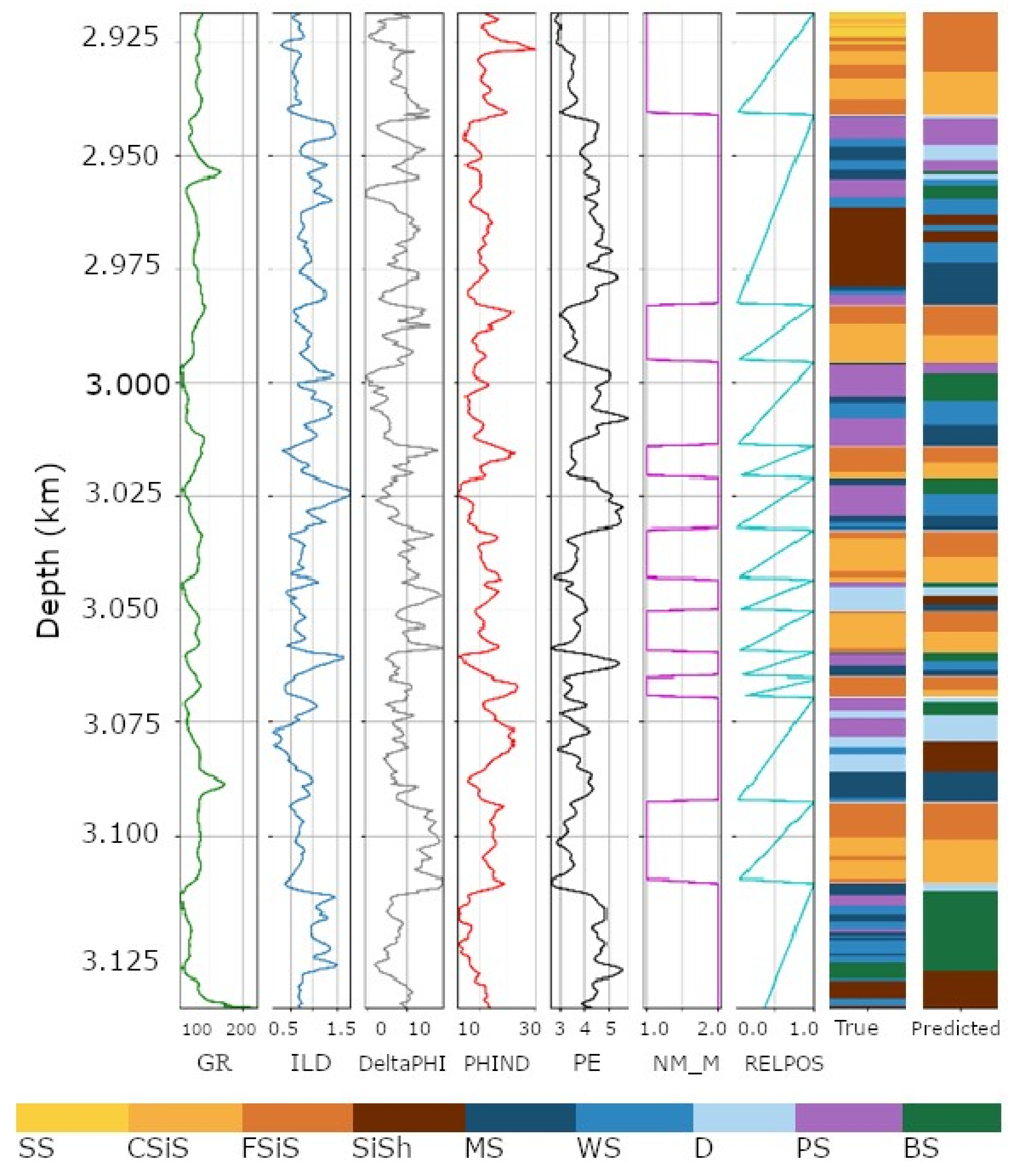
Figure 6 shows an example well, “Kimzey A”, with the lithofacies predicted by previous studies along with the predictions from piecemeal clustering. In the Figure, the wire-line logs are plotted vertically with depth varying alone the
y axis representing the depth of the well.
5. Discussion
5.1. Prediction Effectiveness
To assess the overall effectiveness of the facies classification of the wire-line logs using piecemeal clustering, a number of measures can be considered, such as accuracy, precision, recall, and F1-score. The accuracy of the algorithm was demonstrated in the previous section, where the accuracies were calculated with and without consideration of adjacent facies.
For calculating precision, recall, and F1-score, predictions excluding adjacent facing were used. The precision is the percentage of all correct positive predictions of a class out of all actual positive predictions. Precision is a useful metric when the cost of false positive predictions is very high. Non-marine coarse siltstone (CSiS) was found to give the result with the highest precision, 55.18%, while Non-marine sandstone (SS) was found to give the result with the lowest precision, 48.58% among the non-marine facies. Among the marine facies, phylloid-algal bafflestone (BS) was found to yield the result with the highest precision of 51.97%, while dolomite (D) yielded the lowest precision at 27.89%. The overall precision of 48.98% was calculated by taking the weighted average of all precision values.
The
recall, on the other hand, calculates the percentage of true positive predictions from all positive predictions.
Table 3 shows the recall values for all facies. The overall recall value is calculated by taking the weighted average of all recall values, and was found to be 47.26%.
The F1-score combines both the precision and recall by taking their harmonic mean. The highest F1-score found among non-marine facies was for non-marine sandstone (SS) at 59.10%, while the lowest score found was for non-marine coarse siltstone (CSiS) at 47.85%. Among the marine facies, the highest score was found for phylloid-algal bafflestone (BS) at 63.44%, while the lowest was found for packstone–grainstone (PS) at 35.36%. The overall F1-score was 46.96%.
The variations in precision and F1-score values among non-marine facies were observed to be lower than those for the marine facies. The difference between the highest and lowest values is significantly higher for marine facies. However, the recall values varied for both marine and non-marine facies.
It is noteworthy that efficiency experiences a marked increase when accounting for adjacency facies. This phenomenon is attributed to the constrained size of the dataset, juxtaposed with the substantial heterogeneity present in the field. It is imperative to emphasize that augmenting the input size of the study is integral for enhancing accuracy.
5.2. Comparison with Other Data Clustering Algorithms
The performance of the proposed lithofacies identification algorithm using piecemeal clustering is compared with the performances of the other aforementioned well-known data clustering algorithms in terms of clustering accuracy as well as the correct identification of the number of clusters present in the data. Subjective analyses were also used to compare the performances of the various clustering algorithms. When comparing the mapping accuracy, both accuracies with and without consideration of the adjacent facies are used. The clustering algorithms that are used in the comparison are: K-means, SOM, DBSCAN, RNN-DBSCAN, and HDBSCAN. The use of the K-means, SOM, and DBSCAN algorithms is widespread as these are more generic clustering algorithms, while the RNN-DBSCAN and HDBSCAN clustering algorithms build upon the DBSCAN algorithm while trying to overcome some of its limitations.
All algorithms compared required the setting of various parameters in order to tweak their performances. For example, K-means and SOM require the number of clusters to be specified beforehand, thus making the number of clusters a required input parameter. In the cases of these two algorithms, we assumed that the correct number of clusters was specified so that there was no chance of the number of clusters being incorrectly identified.
The DBSCAN, RNN-DBSCAN, and HDBSCAN clustering algorithms do not require the number of clusters to be a known input. However, we found that when setting the number of clusters to its known true value for any of these three algorithms, the majority of data points were identified as noise, regardless of the values set for the other parameter values input to those algorithms, and thus the resulting clusters were not comparable to those from the proposed piecemeal algorithm. Therefore, we performed a brute-force search over all possible parameter values for DBSCAN, RNN-DBSCAN and HDBSCAN algorithms, while ensuring that the detected number of clusters was close to the true number of clusters to find the optimal parameters giving the best results. For example, DBSCAN uses the value to determine the clusters, RNN-DBSCAN uses neighborhood relationships (i.e., KNN-search) to determine the data density, while HDBSCAN uses minimum spanning trees where the output clusters are determined by the tree parameters and .
Implementations of the
K-means,
SOM, and
DBSCAN clustering algorithms from the MATLAB
® machine learning toolbox were used for the comparative experiments, while the
RNN-DBSCAN package [
53] from the MATLAB
® library was used for
RNN-DBSCAN implementation. Finally, the Scikit Learn Python package [
54] was used in the experiment when using the
HDBSCAN clustering algorithm.
When generating cluster results from the compared algorithms, there were two types of optimization that could be applied: (a) optimize the algorithms to obtain the correct number of clusters and then find the mapping accuracy; or (b) optimize the mapping accuracy and see how many clusters the algorithms can produce. For
K-means and
SOM, the number of clusters must be specified, so it is only possible to optimize them for the mapping accuracy. For
DBSCAN algorithms, it was possible to optimize for both. When optimizing the results for the correct number of clusters, all of these algorithms detected the majority of the data points as noise and produced non-comparable results. Therefore, the results that are optimized for the mapping accuracy were used while keeping the number of clusters close to the known number of clusters, in the event that there is more than one result that provides a similar mapping accuracy. The experiment was run with two different methods, namely with and without splitting the dataset by marine and non-marine lithofacies. Splitting the datasets for all algorithms provided better results.
Table 5 shows the outcome of the comparison. The four rows of the table compare the accuracy of the number of clusters identified by the clustering algorithms, while the rest of the rows compare the mapping accuracy.
DBSCAN,
RNN-DBSCAN, and
HDBSCAN also separate data points as noise. The last row shows how many of the data points are found as noise by these algorithms.
The dominating facies approach previously mentioned was also applied to analyze the clusters generated by the algorithms being compared. It was found that some of the clusters generated by each of the algorithms represent the same dominating facies. At the same time, some of the lithofacies are not found as dominating facies in any of the clusters. When there is more than one cluster representing the same dominating facies, the cluster with the highest number of dominating data points is considered to be the correct mapping for the purpose of comparing accuracy. The first row of the table shows how many clusters each of the algorithms produces, and the second row shows the number of unique facies identified as dominating facies in the clusters. The number of uniquely identified marine and non-marine facies is also reported in rows three and four.
Piecemeal clustering is the only algorithm that uniquely identified all nine facies and also generated only nine unique clusters. SOM and K-means produced nine clusters as the number is given. DBSCAN could not produce nine clusters when optimized for a better mapping accuracy. RNN-DBSCAN and HDBSCAN produced 11 clusters each. HDBSCAN is the best among the algorithms that were able to identify the most unique facies. All of the algorithms compared, except RNN-DBSCAN, produced two unique non-marine facies. For identifying marine lithofacies, HDBSCAN exhibited the best result after piecemeal clustering by finding five non-marine facies.
Comparing the mapping accuracy also reveals interesting facts about the other clustering algorithms. For mapping accuracy, piecemeal clustering yields the best result for marine and non-marine facies. Among the other algorithms, DBSCAN yields the best result. HDBSCAN also produces a similar accuracy to DBSCAN and, at the same time, produces a better result in terms of finding the number of facies. Both DBSCAN and HDBSCAN also produce results close to those produced by piecemeal clustering. The total and adjacent accuracy also follow a similar comparison. DBSCAN and HDBSCAN performed better than the other three algorithms and produced results close to the piecemeal clustering.
5.3. Comparison with Other Machine Learning Methods
While piecemeal clustering outperforms the data clustering algorithms mentioned above, it is important to test how the piecemeal clustering algorithm performs against known machine-learning techniques.
Table 6 compares our results to those from five other machine-learning techniques. Five performance indicators are used for this evaluation: total accuracy, F1-score, marine (M) facies accuracy, non-marine (NM) facies accuracy, and total adjacent accuracy. The techniques examined in this paper are Gaussian naïve Bayes (GNB), support vector machines (SVM), extreme gradient boosting (XGB), label propagation (LP), self-trained label propagation (self-trained LP), and piecemeal clustering. The results for the other algorithms were obtained from the previously published experiment in [
4].
The percentage of correctly predicted wire-line log signatures from non-marine facies is measured by NM facies accuracy. In contrast, the percentage of correctly predicted wire-line log signatures of marine facies is measured by the M facies accuracy. The overall accuracy measures how many wire-line log signatures of marine and non-marine facies were adequately predicted. The total adjacent accuracy evaluates the proportion of accurately predicted log signatures of facies and respective neighboring facies, whereas the F1-score measures the balance between the precision and recall. With regard to the NM facies accuracy, the self-trained LP performed the best, coming in at 59.81%, followed by XGB, which came in at 54.40%, and was then followed by LP which came in at 51.07%, piecemeal clustering came in at 51.68%, SVM (with CV) came in at 50.41%, and finally GNB came in at 49.21%. Because self-trained LP is a sophisticated boosting algorithm that can handle nonlinear connections and has the capacity to capture interactions between various features, it attained the best accuracy. It is a type of level propagation that iteratively boosts accuracy using a self-training methodology. The powerful algorithm XGB (with default) also excels at this task. Self-trained LP outperformed all other methods in terms of M facies accuracy, coming up at 42.22%, followed by piecemeal clustering at 39.21%, SVM with CV at 36.60%, XGB at 34.67%, LP at 34.46%, and GNB at 32.26%. Piecemeal clustering, by virtue of its use of a clustering-based strategy that can spot patterns in the data and group related samples together, also did well on this challenge.
Total accuracy is a crucial parameter for assessing the overall effectiveness of algorithms. Self-trained LP in this study had the highest overall accuracy (50.92%), followed by piecemeal clustering (45.20%). XGB exhibited a performance which was similar to that of piecemeal clustering at 44.43%. SVM with CV also performed close to XGB at 43.43%. LP and GNB, on the other hand, performed the worst among all these algorithms, at 42.67% and 40.64%, respectively. Due to their capacity for handling unbalanced and noisy data as well as their capacity to learn from unlabeled data, self-trained LP and piecemeal clustering did well for this criterion.
The F1-score is another important metric that balances precision and recall. It gauges how well a model’s predictions balance positive predictive value (precision) with sensitivity (recall). For each of the machine learning methods tested in this study, F1-scores were determined. The self-trained LP had the highest F1-score in this study with 49.35%, followed by piecemeal clustering (46.96%), XGB (42.33%), SVM with CV (39.50%), LP (with default) (35.56%), and GNB (35.39%). Due to their ability to deal with unbalanced data and their capacity to learn, self-trained LP (with default) and piecemeal clustering performed well for this criterion.
Overall, piecemeal clustering has a total adjacent accuracy of 81.90%, indicating that, in most cases, the model correctly predicted the facies. While other algorithms did better than piecemeal clustering when considering the adjacent facies, piecemeal clustering was better than all other algorithms except self-trained LP when adjacent facies were not considered. In addition to that, when we look at the precision, recall, and F1-score for each facies, we can see that the piecemeal clustering performs better in predicting certain facies such as non-marine sandstone (SS) and phylloid-algal bafflestone (BS) and performs poorly in predicting other facies such as dolomite (D) and packstone-grainstone (PS). Therefore, it is important to consider these metrics when evaluating a model’s performance and making any decisions based on its predictions. It is important to note that, in these comparisons, the evaluation is specifically directed towards supervised and semi-supervised algorithms, both of which autonomously train themselves utilizing known outcomes. This intrinsic characteristic leads to the anticipation of higher accuracy results. However, it is important to acknowledge the inherent constraints associated with the utilization of supervised or semi-supervised clustering approaches, primarily attributed to the limited availability of labeled data. The generation of such data is not always feasible and, when possible, entails significant time and cost investments. One unique advantage of piecemeal clustering is that it clusters the dataset without requiring any labeled data and produces tight clusters. This advantage allows piecemeal clustering to be more useful for wells lacking core and thin slice samples. As a result, it is a significantly less expensive option in comparison to other methods while still producing comparable results.
5.4. Research Question Validation
The study was conducted to validate two research questions as presented in
Section 1. Based on the provided information, it is possible to assess whether the research questions were answered.
The first research question was ‘is it possible to identify lithofacies using the piecemeal clustering algorithm without prior knowledge of the number of lithofacies in the data?’ The algorithm identified three non-marine lithofacies and six marine lithofacies from the dataset, one for each of the nine lithofacies from the known results. It was 100% accurate in identifying the number of lithofacies. The piecemeal clustering algorithm outperformed other data clustering algorithms. In addition, based on the provided results, which included accuracy, precision, recall, and F1-score, it is possible to assess the effectiveness of identifying lithofacies using the piecemeal clustering algorithm with other machine learning techniques, when there is no prior knowledge of the number of lithofacies in the data. The precision measures the percentage of correct positive predictions of a class out of all actual positive predictions. The precision values vary for different lithofacies, with non-marine coarse siltstone (CSiS) yielding the result with the highest precision at 55.18% and non-marine sandstone (SS) receiving the result with the lowest precision at 48.58% among the non-marine facies. For marine facies, phylloid-algal bafflestone (BS) received the result with the highest precision at 51.97%, while dolomite (D) received the result with the lowest precision at 27.89%. The overall precision, calculated as a weighted average of all precision values, was 48.98%, for the piecemeal clustering algorithm.
The recall calculates the percentage of true positive predictions out of all positive predictions. The recall values for all facies are provided in
Table 3, and the overall recall value, calculated as a weighted average, was found to be 47.26% for piecemeal clustering.
The F1-score combines both precision and recall, taking their harmonic mean. Among the non-marine facies, non-marine sandstone (SS) resulted in receiving the highest F1-score at 59.10%, while non-marine coarse siltstone (CSiS) received the result with the lowest at 47.85%. For marine facies, phylloid-algal bafflestone (BS) received the highest F1-score at 63.44%, while packstone–grainstone (PS) received the lowest at 35.36%. The overall F1-score is calculated to be 46.96% for piecemeal clustering.
Based on these aforementioned results, the use of the Piecemeal Clustering algorithm for lithofacies identification without prior knowledge of the number of lithofacies in the data achieved reasonable precision, recall, and F1-scores. While the values may vary for different lithofacies, the overall performance indicates that unsupervised machine learning algorithms, such as piecemeal clustering, have the potential to effectively identify lithofacies.
The second research question was ‘does the piecemeal clustering algorithm yield comparable results to other data clustering algorithms, and supervised and semi-supervised machine learning techniques?’ Based on the provided information, the answer to this question can be inferred to be positive. The text mentions comparisons of the results obtained from different data clustering algorithms and machine learning techniques, including unsupervised piecemeal clustering. Among supervised algorithms, the comparison includes Gaussian naïve Bayes (GNB), support vector machines (SVMs), extreme gradient boosting (XGB), and semi-supervised algorithms including label propagation (LP) and self-trained label propagation (self-trained LP). This study describes the evaluation of these algorithms using various performance indicators, such as total accuracy, F1-score, marine and non-marine facies accuracy, and total adjacent accuracy. This found that piecemeal clustering performed better than the commonly used data clustering algorithms, and reasonably well compared to the other machine learning techniques in terms of accuracy, F1-score, and overall performance. Therefore, this suggests that unsupervised data clustering, represented by piecemeal clustering, can provide similar results compared to supervised and semi-supervised clustering algorithms for the identification of lithofacies. However, it is important to note that the evaluation and comparison were specific to the dataset and algorithms used in this particular study. The performance of different algorithms may vary depending on the dataset characteristics and the specific problem domain. It is recommended to consider these factors when selecting an appropriate algorithm for a given task.
6. Conclusions
In this study, the effectiveness of a novel unsupervised clustering algorithm, piecemeal clustering, was explored for identifying lithofacies without prior knowledge of the number of lithofacies in the data. The research questions address two important issues: (a) the feasibility of identifying lithofacies using the piecemeal clustering algorithm and (b) the comparison of the piecemeal clustering algorithm with other data clustering algorithms, supervised and semi-supervised machine learning techniques. By evaluating the algorithm’s performance using various metrics, such as accuracy, precision, recall, and F1-score, valuable insights into its capabilities were gained.
The results obtained from our experiments provide evidence that Piecemeal Clustering holds promise for lithofacies identification. Piecemeal clustering outperformed other commonly used data clustering algorithms and was competitive with known machine learning techniques. The evaluation included five performance indicators: total accuracy, F1-score, marine (M) facies accuracy, non-marine (NM) facies accuracy, and total adjacent accuracy. While some machine learning algorithms, such as XGB and self-trained LP (default), outperformed piecemeal clustering in specific metrics like non-marine facies accuracy and marine facies accuracy, the overall performance of piecemeal clustering was notable.
It is also important to note that the effectiveness of the piecemeal clustering algorithm varied across different lithofacies. On some lithofacies, such as non-marine sandstone (SS) and phylloid-algal bafflestone (BS), the algorithm demonstrated higher precision, recall, and F1-score, indicating that the algorithm performed better in predicting these facies. On the other hand, lithofacies like dolomite (D) and packstone–grainstone (PS) posed challenges to the algorithm, resulting in lower predictive performance. Therefore, it is crucial to consider these variations and assess the algorithm’s performance for each lithofacies category individually. It is imperative to acknowledge that the present study was conducted on a restricted set of wells, precisely 10 in number, owing to its accessibility within the public domain. The constrained availability of data may, in turn, constrain a comprehensive exploration of field heterogeneity through data clustering algorithms. To augment the efficacy of identifying lithofacies using data clustering techniques, further experiments on larger datasets are recommended. Such endeavors are anticipated to further understand the approach’s effectiveness in delineating the characteristics of lithofacies within diverse geological formations.
To further enhance the effectiveness of unsupervised clustering algorithms for the identification of lithofacies, several potential avenues can be explored. Firstly, incorporating additional variables or features derived from wire-line log measurements could provide valuable information and improve the algorithm’s accuracy. Parameters such as gamma ray (GR), resistivity (RT), neutron porosity (NPHI), and density (RHOB) have been widely used in lithofacies classification and could be considered as inputs to the clustering algorithm.
This study also demonstrated the potential of unsupervised data clustering algorithms for lithofacies identification using one state-of-the-art unsupervised data clustering algorithm. In the future, a more comprehensive study can also be conducted, employing other unsupervised data clustering algorithms on various wire-line log datasets. Furthermore, exploring advanced techniques for handling imbalanced and noisy data could address the challenges associated with certain lithofacies categories. Techniques such as data resampling, feature engineering, or applying ensemble methods might enhance the algorithm’s performance and accuracy, particularly for lithofacies with limited representation in the dataset. Additionally, incorporating domain-specific knowledge and geological constraints into the algorithm could contribute to better lithofacies identification. By integrating geological principles, such as stratigraphic layering, facies associations, and spatial patterns, the algorithm could leverage this information to guide the clustering process and improve the accuracy of lithofacies assignments.
In conclusion, this study demonstrates the potential of unsupervised clustering algorithms, particularly piecemeal clustering, for lithofacies identification without prior knowledge of the number of lithofacies. While the algorithm achieved competitive results compared to known machine learning techniques, its performance varied across different lithofacies categories. By considering additional variables, addressing data imbalances, and incorporating domain-specific knowledge, the algorithm’s effectiveness can be further enhanced. These findings contribute to the field of geoscience research and open up new opportunities for automated lithofacies identification in various applications, such as reservoir characterization and geological modeling. Future studies should continue to explore these avenues and refine the presented algorithm, and potentially others, to achieve even more accurate and robust lithofacies classification results.


