
Applications of Machine Learning in Subsurface Reservoir Simulation—A Review—Part II

1
School of Mining and Metallurgical Engineering, National Technical University of Athens, 15780 Athens, Greece
2
Institute of Geoenergy, Foundation for Research and Technology-Hellas, 73100 Chania, Greece
*
Author to whom correspondence should be addressed.
Energies 2023, 16(18), 6727; https://0-doi-org.brum.beds.ac.uk/10.3390/en16186727
Submission received: 17 July 2023
/
Revised: 7 September 2023
/
Accepted: 18 September 2023
/
Published: 20 September 2023
(This article belongs to the Special Issue Artificial Intelligence/Machine Learning Applications in the Oil and Gas Industry)
Abstract
:In recent years, Machine Learning (ML) has become a buzzword in the petroleum industry, with numerous applications which guide engineers in better decision making. The most powerful tool that most production development decisions rely on is reservoir simulation with applications in multiple modeling procedures, such as individual simulation runs, history matching and production forecast and optimization. However, all of these applications lead to considerable computational time and computer resource-associated costs, rendering reservoir simulators as not fast and robust enough, and thus introducing the need for more time-efficient and intelligent tools, such as ML models which are able to adapt and provide fast and competent results that mimic the simulator’s performance within an acceptable error margin. In a recent paper, the developed ML applications in a subsurface reservoir simulation were reviewed, focusing on improving the speed and accuracy of individual reservoir simulation runs and history matching. This paper consists of the second part of that study, offering a detailed review of ML-based Production Forecast Optimization (PFO). This review can assist engineers as a complete source for applied ML techniques in reservoir simulation since, with the generation of large-scale data in everyday activities, ML is becoming a necessity for future and more efficient applications.
1. Introduction
The primary objective of the petroleum industry and its applications is to discover and exploit oil and gas reserves to ensure affordable energy access, meet global energy demands, and maximize profits. Reservoir engineers rely on subsurface reservoir simulation as a vital tool to accomplish these goals, which plays a crucial role in gaining a comprehensive understanding of reservoir behavior, facilitating detailed analysis, and optimizing recovery processes. Simulation is used in various planning stages, reservoir development, and management to enhance the efficiency of extracting hydrocarbon reserves from underground reservoirs.
As discussed in detail in Part I [1] of the present review, reservoir simulation integrates principles from physics, mathematics, reservoir engineering, geoscience, and computer programming to model the hydrocarbon reservoir performance under various operating conditions. The reservoir simulator’s output, typically comprised of the spatial and temporal distribution of the pressure and phase saturation, is introduced to the simulation models of the following physical components in the hydrocarbon production chain, including those that produce fluids at the surface (wellbore) and process the reservoir fluids (surface facilities), thus allowing for the complete modeling system down to the sales point [2,3]. Reservoir simulators are the mathematical tools built to accurately predict all the physical fluid flow phenomena inside the reservoir with a reasonable error margin, thus acting as a “digital twin” of the physical system.
Simulators estimate the reservoir’s performance by solving the differential and algebraic equations derived from the integration of mass, momentum, and energy conservation together with thermodynamic equilibrium, which describe the multiphase fluid flow in porous media. By using numerical methods, typically finite volumes, these equations can be solved throughout the entire reservoir model for variables with space- and time-dependent characteristics, such as pressure, temperature, fluid saturation, etc., which are representative of the performance of a reservoir [3].
For this task, a static and a dynamic reservoir model must be first set up. A static reservoir model is a three-dimensional representation of a reservoir’s geological properties, such as the porosity, permeability, and rock type. It is created using geological, well, and seismic data together with a thorough interpretation, providing an approximate “snapshot” of the real reservoir at a specific time [4,5,6]. On the other hand, a dynamic reservoir model is a time-dependent simulation of fluid flow in the reservoir. It builds upon the static model by incorporating production history, fluid properties, and reservoir management strategies. The dynamic model is employed to predict reservoir behavior, optimize production, and assess various development scenarios, such as enhanced oil recovery techniques and the impact of drilling new wells.
To integrate the static and dynamic reservoir models, the simulator divides the reservoir into many cells (grid blocks), or otherwise into a large number of space and time sections, where each cell is modeled individually (Figure 1). The simulation method assumes that each reservoir cell behaves like a tank with uniform pressure, temperature and composition of the individual phases for each specific time. During the fluid flow, each cell communicates with all neighboring cells to exchange mass and energy. Subsurface reservoir models can be highly complex, exhibiting high inhomogeneity, a vast variance of the petrophysical properties, such as porosity and permeability, and peculiar shapes capturing the structure and stratigraphy of the real reservoir.
Typically, reservoir simulations employ black oil or compositional fluid models to simulate the thermodynamic behavior of fluids. Black oil models are commonly used for simple phase behavior phenomena, providing a straightforward and reasonably accurate approach [7,8]; however, in cases of production forecasting and optimization applications, especially for complex phenomena, such as CO2 injection for Enhanced Oil Recovery (EOR), fully compositional simulations are necessary to monitor detailed changes in fluid composition [9]. Compositional reservoir simulations involve stability and flash calculations using an Equation of State (EoS) model to determine the number and composition of fluid phases in each grid block. These calculations are computationally demanding, require high-performance systems to be executed successfully and, therefore, consume a significant portion of the simulation’s CPU time, as both problems need to be solved repeatedly for each discretization block, at each iteration of the non-linear solver and for each time step [10,11].
Once the reservoir model has been set up, the most computationally expensive applications of simulation, History Matching (HM) and Production Forecast and Optimization (PFO) of future reservoir performance, can be performed. HM is the most important step preceding the reservoir performance optimization and is widely covered in Part I of the present review. When it comes to predicting and optimizing reservoir performance under various production scenarios, reservoir simulation plays a vital role. It is an essential tool for production management and techno-economic planning, as these activities heavily rely on accurate reservoir performance predictions. Forecasting entails making predictions about future production rates and the distribution of reservoir pressure and saturation, which rely on historical data, reservoir characteristics, and other pertinent factors. It helps operators make informed decisions regarding resource allocation, production planning, and investment strategies. Optimization, on the other hand, focuses on maximizing production efficiency and profitability while minimizing costs, downtime, and environmental impact. It involves analyzing production processes, well performance, and reservoir behavior to identify areas for improvement. PFO techniques may include wellbore management, enhanced oil recovery methods, production scheduling, and asset management strategies [12].
While the aforementioned PFO applications are central to reservoir engineering, they pose challenges in terms of their heavy computational cost. The iterative nature of the calculations involved makes the problem under investigation computationally demanding, becoming particularly cumbersome for extensive and detailed reservoir models, where the increasing number of grid blocks, the diverse reservoir parameter distribution, and the complex well operation schedules significantly prolong the calculations performed by traditional non-linear solvers [13]. Thus, to achieve accurate forecasts and effective optimization, oil and gas operators must devise efficient ways to deal with these types of problems, such as Machine Learning (ML) techniques, to make decisions, optimize production operations, and adapt to changing market conditions, ultimately maximizing the value of oil and gas assets.
The increasing volume of data has prompted extensive research across engineering disciplines to extract meaningful patterns and insights, since human cognition alone is often insufficient to process and comprehend this vast amount of information [14]. In recent years, data-driven ML techniques have gained significant traction and proven successful in supporting field development plans. These techniques enable the development of models that capture the essence of physical problems without the need to explicitly express fundamental laws mathematically. Typically, these models take the form of functions or differential equations that provide approximate and partially imprecise results, offering fast, robust, and cost-effective solutions [15,16,17].
ML offers an automated methodology for constructing numerical models that can learn and identify patterns from observed or synthetically derived data, reducing the need for extensive human intervention and facilitating the decision-making process. ML can help in analyzing vast and complex datasets, ranging from seismic data to production records. By uncovering complex patterns and relationships, it significantly refines reservoir characterization, providing a more comprehensive and accurate representation of subsurface conditions. This improved understanding minimizes uncertainties associated with reservoir properties, boundaries, and heterogeneity, thus elevating the quality and reliability of the model. Furthermore, ML’s predictive capabilities can be used to optimize production strategies. By analyzing real-time production data and considering the complex interplay of variables, algorithms are able to devise optimal operational plans. This results in maximizing recovery rates, minimizing operational costs, and optimizing production.
As presented in Part I of the present review, the most common types of ML are Supervised Learning (SL), Unsupervised Learning (UL), and Reinforcement Learning (RL). Furthermore, the development of an ML model consists of three primary steps. First, data is collected into a large dataset, as its quantity impacts the model’s accuracy, which is used for the model’s training process. Second, data preparation, including dimensionality reduction and handling outliers or missing data, is crucial for ensuring prediction precision. Finally, the model is trained using input variables and the desired output for supervised learning, which are assessed on the model’s ability to effectively predict and classify previously unseen data.
In the context of subsurface reservoir simulation, traditional simulators generate large data ensembles offline, for various conditions, to train ML models. Unlike most ML applications, the derived data comes from computational processes rather than experiments, resulting in noiseless information. Once trained, the ML model serves as a ‘’digital twin’’ of the reservoir, offering fast and accurate predictions about past, present, and future performance. This allows the model to address various problems and support decision making more efficiently [18,19].
This review discusses the approaches of ML-based reservoir simulations to provide a wide perspective on the state-of-the-art methods currently in use for PFO applications, as HM and individual reservoir simulation runs were extensively covered in Part I of the present review. More specifically, the modeling of subsurface reservoirs is covered extensively in Part I by incorporating a review of proxy models (SRMs) and ML models that focus on CPU time-intense sub-problems while maintaining the rigorous differential equation-solving method. The most pronounced application in this category is the handling of the phase equilibrium problem in its black oil or compositional form which needs to be handled numerous times during the reservoir simulation run.
In contrast to HM methods that follow a rather straightforward approach [1], ML-based techniques for PFO offer a broad spectrum of applications. These applications include optimizing the oil and gas cumulative or individual well production, predicting the water breakthrough time in water-flooding scenarios, forecasting CO2 injection-related sweeping and recovery, and identifying optimal locations for new wells to enhance the future production.
In this part of the present review paper (Part II), the ML methods for the subsurface reservoir simulation reviewed are categorized based on the context of the problem under investigation and the ultimate purpose of each reviewed method. Section 2 reviews ML methods that serve PFO applications and Section 3 concludes the present review.
2. Machine Learning Strategies for Production Forecast and Optimization Applications
A precise prediction of oil recoveries and determination of the optimal parameters that can maximize production or Net Present Value (NPV) is crucial to establishing techno-economic assessments for various production operations. However, obtaining precise predictions using standard reservoir simulation packages can be very cumbersome, since most recovery operations are governed by the high non-linearity of the flow equations and the complex spatial distribution of the reservoir parameters (e.g., porosity, permeability, saturation, etc.). Furthermore, even in cases where the underlying relationship between oil rate and reservoir parameters can be easily established, the limited availability of data, which is usually the case, especially for newly discovered reservoirs, imposes an increased uncertainty on the simulations. On the other hand, when the number of reservoir parameters is huge and much data are available, it is usually hard and impractical to reach an optimal solution, since the models can be of very high dimensionality. Consequently, building robust and precise PFO models using the available data is of major importance to reservoir engineers since, that way, they can gain better insights about the reservoir performance and thus, plan optimally for any reservoir management and field development strategies.
As Bao et al. [20] quote, “Many methods have been developed to estimate the oil production rate in an accurate and fast manner, such as decline curve (DCA) and well test analysis, numerical /analytical reservoir stimulation for both conventional and unconventional reservoirs, but the challenge lies in the noise and missing data and anomalies that could happen in the field”. While simple reservoir simulations, material balance, and a nodal analysis can be sufficient for small production systems, large complicated systems need a more advanced approach based on multiple simulation runs that, as already mentioned, can be extremely time-consuming [21]. All the above constraints have inspired engineers to consider new and novel alternatives that can mitigate the CPU time intensity of reservoir simulators to a great extent.
The ever-growing data volume in the petroleum industry has led to the widespread use of ML techniques, especially in PFO applications. Different ML methods are widely used to obtain insights into various operational and design processes (i.e., CO2 injection into the reservoir for EOR purposes or injection well spacing optimization to improve recovery, respectively) using data obtained from the field (gauges, flow meters, etc.), sampling, logging, or experimental procedures. These methods can be adapted to obtain hydrocarbon predictions and optimize many reservoir- and production-related parameters, thus leading to an effective production optimization in a fraction of the time that would otherwise be needed using traditional reservoir simulators.
However, since data volumes have grown significantly and engineers need to deal with large amounts of data flows, some of them containing non-useful information, screening out those non-informative features is a crucial process in the construction of a reservoir model using ML, aimed at enhancing the model’s predictive accuracy and preventing the introduction of noise or overfitting (Figure 2). In the context of reservoir modeling, where accurate predictions are paramount for efficient resource management, this process involves a comprehensive evaluation of each feature’s contribution to the model’s performance. Starting with an exploration of the dataset’s characteristics and distributions, techniques such as feature importance analysis, correlation assessments, and domain knowledge are employed. By leveraging algorithms that quantify feature importance based on their impact on predictive accuracy, identifying correlations between features and the target variable, and applying statistical tests, the model developer can determine the relevance of each feature. Moreover, considering the inter-feature relationships, redundant or highly correlated attributes are identified and streamlined. Furthermore, the collaboration with domain experts can significantly aid in discerning irrelevant features that may not carry meaningful geological or geophysical significance. Through this systematic approach, non-informative features are identified, and dimensionality reduction techniques, such as regularization and dimensionality reduction algorithms, help prioritize informative attributes. This iterative process ensures that the reservoir model is built upon a foundation of relevant features, leading to enhanced precision, improved generalization, and a robust representation of the reservoir dynamics.
It should further be noted that a great number of the methods discussed in this review are based on an existing and already history-matched reservoir model rather than directly on field data. In such cases, the PFO operator is already aware that that uncertainty has been compromised through history matching, and the reservoir simulator is supposed to act as the digital twin of the real reservoir. Therefore, the incorporation of irrelevant information to the ML models is automatically skipped as the data introduced to the machines is taken from the physics-driven reservoir simulator.
Usually, for the application of ML models for PFO, two kinds of problems are considered. The first class is the so-called forward problem, in which ML models use reservoir and design parameters (e.g., fixed Bottom Hole Pressures—BHPs or production rates, injection rates and/or gas stream composition for various EOR operations, well spacing, etc.) as inputs to predict the response of the system (e.g., future production rates or NPV). Those models act as direct prediction proxies for fluid production and pressure response forecasts. The second class is the inverse design problem, where ML models predict the necessary design parameters to obtain a desired system response (i.e., production rate) [22].
The ML methodologies reviewed in this section are divided into seven distinct categories, namely production optimization and production forecast concerning conventional reservoirs, production forecast for unconventional reservoirs, EOR/Sequestration projects, heavy oil reservoirs, gas condensate reservoirs, and a few applications on flow assurance problems. Each production forecast category is split into static/dynamic models, since each type is developed using a different ML technique and presents a different output (time-static and time-dependent values, respectively).
2.1. Production Optimization of Conventional Oil Reservoirs
2.1.1. Production Optimization Based on ANNs
Starting with ML production optimization applications for conventional primary and secondary stage oil fields (i.e., non-complex reservoirs without an EOR project implementation), Koray et al. [23] developed simple Artificial Neural Network (ANN) models for the oil recovery optimization by exploiting different field development scenarios, namely normal depletion and water-flooding. ANNs are considered ideal candidates for such problems, as their architecture enables the quick capture of complex relationships within data. As depicted in Figure 3, they consist of interconnected nodes, or neurons, organized into layers that process input data and produce output predictions. This architecture excels in recognizing patterns, especially in cases where the relationships between input variables and desired outputs are nonlinear. For simple optimization tasks, ANNs can efficiently learn from historical production data and identify optimal combinations of operational parameters to achieve specific production goals. The authors used well locations, injection rates, production/injection BHPs, and water cuts of each development scenario as input to forecast the cumulative oil production for 15 years. By applying various test scenarios to the trained ANN, it was concluded that the water-flooding development strategy was the one that maximized oil production.
Zangl et al. [24] and Andersen [25] developed a similar approach by coupling a Genetic Algorithm (GA) with ANNs to achieve production optimization while reducing the computational time required by only running a limited amount of simulations. More specifically, Zangl et al. [24] trained the ANN using information about the wellhead pressure and temperature, choke size, and BHP as input and oil production as output, as obtained from simulation realizations, whereas Andersen [25] used production and injection well rates as input and total oil production as output. That way, as flow rates are regulated, different cumulative production values can be gained. Once the models are trained and validated, their output is used as a very close approximation to the simulator’s output and, that way, the GA is then employed to perform the optimization.
Although there exist many mathematical algorithms and optimization tools that are usually employed to determine the optimal number and placement of production wells [26,27], Centilmen et al. [28] moved into the ML field and built an ANN, focusing on the well placement that achieves the optimum production. The authors used two input options, one stationary (well locations) and one input related to the problem under investigation (the distance between two wells, production time, etc.) to determine each well’s production (output). The model, after being trained and validated, was used to optimize the location for the new wells that must be drilled. Doraisamy et al. [29] further improved Centilmen et al.’s work by coupling soft and hard computing methodologies to efficiently determine the optimum well placement while exploiting the processing power of back-propagation and recurrent networks and the precise description of the related physics, respectively. To achieve that, the authors trained the ANN using available real data from the oil field and data generated numerically by a simulator (coordinates of the existing, training and new wells, distances between the new and the existing wells, etc.) to determine the oil rate of each well configuration. Min et al. [30] developed an ANN embodying the productivity potential to determine the optimum new well placement that maximizes the total production. The authors introduced the productivity potential to decrease the input dataset size, since it indirectly contains many reservoir parameters (e.g., porosity, permeability) that otherwise should have been introduced individually. Thus, the model’s input consisted of time-related parameters, the wells’ distances, and the productivity potential to produce the output that is the cumulative production.
Among all secondary production schemes, water-flooding is the most commonly used one, since it is a relatively easy-to-implement process with better economics than gas injection and can effectively assist oil production. Teixeira et al. [31] developed two ANN models of varying configurations to uncover the relation between total oil production (output) and control parameters (input) for the optimization of the production strategy of a reservoir under water-flooding. The authors used water injection rates, oil production rates, and BHPs as input to predict the optimum future oil production. The proposed models were shown to perform satisfactorily; however, the results exhibited a noisy behavior in both models that could disturb the optimization process.
All of the above ANN-based techniques exhibit high efficiency in optimizing production since the quality of the predicted solutions is comparable to the performance of the original reservoir simulator when utilized to exhaustively optimize the production. Furthermore, the use of those models leads to a great decrease in the total CPU time, proving that the developed approaches can help solve optimization problems and increase the economic benefits of an oil field.
2.1.2. Production Optimization Based on Other Methods Other Than ANNs
Besides ANNs, many alternative ML methods have also been developed to effectively assist production optimization, such as Extreme Gradient Boosting (XGB), which is an ensemble learning algorithm (designed for both classification and regression tasks) that consists of a collection of Decision Trees (DTs) and falls under the category of gradient boosting methods. XGB operates through an iterative procedure (Figure 4) that transforms a training dataset into a predictive model. It starts by initializing the prediction with a constant value, typically the mean of the target variable. Then, it constructs a DT using the training dataset, aiming to minimize the gradient of the loss function. This tree captures patterns in the data and predicts residuals—differences between the actual and predicted values. The predictions from this tree are then multiplied by a small learning rate, representing the step size towards the optimal prediction. The residuals are updated using the multiplied predictions. This process iterates, with each new tree learning from the residuals left by previous trees. Finally, the predictions from all the trees are combined by summing them up, resulting in the final prediction. This sequential aggregation of predictions and residuals forms the basis of XGB’s ensemble algorithm, which efficiently captures complex relationships in data while ensuring high predictive accuracy.
Chai et al. [33] developed such an ML model, along with an ANN as well as a simpler MultiVariate Regression (MVR) model for comparison reasons, to optimize injection and production rates (output) and, therefore, optimize the development strategy of the field. First, a conventional simulator was utilized to run several production schemes and to obtain a training dataset consisting of heterogeneous porosity and permeability fields and BHPs as input and injection and production rates as output, to train the selected ML models. The Karhunen–Lo’eve expansion method was utilized to reduce the parameter space and, thus, reduce the complexity of the model. The results showed that both the XGB and ANN presented quite high and invariable accuracy when compared to the MVR method, even for the case of relatively small datasets, although the ANN presented a superior performance when larger datasets were considered. After the models were trained and tested, the well controls (BHPs for both injection and production wells) were optimized using three search-based algorithms, Particle Swarm Optimization (PSO) [34], GA, and a combination of these two, called Genetical Swarm Optimization (GSO) [35]. The main idea was that these methods provide a quick and agile solution to the optimization problem and the model can provide fast results based on the given input parameters. The results showed that GA and GSO generated better results when compared to PSO.
Guo et al. [36] developed one of the first Least Square Support Vector Regression (LSSVR) models to identify the optimum well controls (i.e., well operating conditions) that maximize the NPV and, thus, optimize the field’s production. LSSVR is an extension of the Support Vector Machine (SVM) algorithm, tailored to regression scenarios, and uses support vectors that seek to find a regression function that can accurately predict target values based on input features. To handle nonlinear relationships, LSSVR employs kernel functions to implicitly transform data into a higher-dimensional space, allowing the algorithm to capture intricate patterns in the data. Guo et al. [36] run conventional reservoir simulations, the number of which is selected with the help of the Latin Hypercube (LH) sampling method in order to build the training dataset for the LSSVR model, which consists of various well operating conditions (water injection rate for injectors; BHPs for producers) as input and NPV values as output. After the dataset is generated, the forward LSSVR model is used for optimization in conjunction with a steepest-ascent algorithm. The results were compared with the ones of the Stochastic Simplex Approximate Gradient (StoSAG) optimization algorithm [37] and conventional simulations, showing that the total computational cost is substantially reduced and, most importantly, the model’s performance presents very similar results to the CPU time-expensive StoSAG algorithm and the simulator.
Al-Lawati et al. [38] developed an unsupervised ML method to optimize gas production by determining the most favorable production parameter setup. The unsupervised model was developed to identify well clusters with comparable production profiles, which are then utilized to determine the actions that must be taken (drilling, choke size, etc.) to obtain optimal production. The model was trained using the daily gas production, drilling and completion data, and other well control data (e.g., choke size). One of the advantages of the proposed procedure is that the model can be adapted accordingly to be used as an optimization approach for many applications, such as budget handling or emissions control. Shirangi [39] developed unsupervised fast NPV models using ANNs or Support Vector Regression (SVR) and trained with well controls as input to predict NPV values, which are then optimized using a pattern search algorithm. Before the models’ development, the authors performed a kernel clustering technique to select the minimum set of conventional simulation runs required to best represent the uncertainty of the whole set. Since the quality of an ML model depends highly on the quality of the training dataset, once the models were trained, the authors added new training data points close to the optimum value to train a new model. The procedure (getting improved optimum and enhancing the training population) is repeated until the desired error margin is reached. Both models provided significant computational time reduction and accurate results.
Finally, Gu et al. [40] developed an XGB model to predict the water cut (output) of producing water-flooded wells, trained with dynamic production data (e.g., water injection, delivery capacity, liquid production, etc.) as input. The input was preprocessed using the Spearman rank correlation analysis [41], which determines the correlation between two parameters, and, in the present case, the correlation between water cut and dynamic attributes. After the model is trained and tested, a differential evolution algorithm is utilized for the optimization of the injection-production strategy by minimizing the obtained water cut. The results showed a significantly improved water-flooding process.
2.2. Production Forecasting of Conventional Reservoirs
Forecasting oil production and production economic-related parameters (e.g., NPV) equips oil and gas operators with a rigorous plan to reduce risks that might alternatively affect operational and financial decisions. The task of conducting trustworthy production predictions can be burdensome and extremely time-consuming [42], especially when numerical simulators demand a thorough reservoir static and dynamic description. Reservoir simulation demands certainty related to input data, validated through HM, which is a time-consuming approach that does not always guarantee uncertainty reduction. Furthermore, all readily available empirical correlations that calculate oil production volumes are developed using field data and, thus, they cannot be adapted and used to every reservoir around the world due to their varying complexity and heterogeneity [43].
ML methods, mostly ANNs, are widely utilized for production prediction purposes since they can provide fast and robust models that tend to overcome the drawbacks of conventional numerical simulators. Production prediction ML-based techniques can be roughly divided into two groups (Figure 5). The first is based on building ML models that predict reservoir properties and behavior based on the current state of the reservoir without considering temporal changes. It provides a snapshot of the reservoir at a specific moment, which is useful for analyzing static scenarios or short-term predictions. The training procedure for a static model involves using a dataset that captures various reservoir parameters at a particular time. The model learns the relationships between these parameters and the target variable, such as production rates or pressure, without accounting for historical data or temporal trends. The trained model can then predict reservoir outcomes based solely on the current input parameters.
The second group, on the other hand, accounts for the temporal evolution of reservoir behavior. It considers how reservoir properties change over time and how different stages influence each other. Dynamic models use time series data to capture historical patterns, making them suitable for long-term predictions and understanding reservoir dynamics. The training procedure for a dynamic model involves creating a dataset that incorporates time sequences of various reservoir parameters and corresponding outcomes. Techniques such as Recurrent Neural Networks (RNNs) or Time Series models are commonly used to handle the temporal dependencies. These models learn to predict future reservoir behavior by considering historical data points and their sequential relationships and are very efficient in predicting future time series values governed by nonlinear dynamics without the need to include the effects of any reservoir physical process, hence requiring significantly fewer input data [44].
Although both groups aim at predicting time-related data, the terms “static” and “dynamic models” are used respectively to distinguish between those predicting distinct characteristic values or time series.
2.2.1. Static Machine Learning Models
For the first category, Gharbi et al. [45] were among the first to develop an ANN to forecast the oil recovery at breakthrough for an immiscible water displacement process. The authors trained a simple ANN model using five dimensionless scaling parameters as input (mobility ratio, capillary to viscous forces ratio, gravitational to viscous forces ratio, length–thickness aspect ratio, and dip angle number) and oil recovery as output. Their work can be thought of as a generalization of the Buckley–Leverett theory using ML. Weiss et al. [46] developed an ANN model to forecast oil production for a water-flooding operation, with the help of the Fuzzy ranking method [47] that is utilized to determine the ANN input parameters (unitized area, permeability, water–oil ratio, porosity, initial BHP, and Gas to Oil Ratio—GOR). Cao et al. [48] also developed an ANN model using production-related data, to forecast the future production of existing wells, as well as of new wells by taking advantage of the production history of neighboring wells sharing similar characteristics, geological maps, pressure data, and operational constraints. In Fan et al. [49], ANN models were successfully built to forecast production using static reservoir parameters (porosity and thickness), water saturation, and well drainage areas. Simple ANN models were also developed by Elmabrouk et al. [50] and Sun et al. [51] to provide oil production forecasts, using real historical production data. The results of the above simple ANN-based models showed that they could accurately predict future oil production since they presented comparable results to conventional simulators in a fraction of the time that it would otherwise be required.
Apart from ANNs, many other methods can be used for production prediction purposes, such as Random Forests (RFs) and Gradient Boosting Regressors (GBRs). RF is a highly effective ensemble ML method used for both classification and regression tasks. It functions by combining the predictions of multiple individual DTs to achieve higher accuracy and generalization, as can be observed in Figure 6. Each tree is trained on a different subset of the data, introducing variability and reducing the risk of overfitting. During training, subsets of the data are randomly selected with replacement through a process called bootstrapping. Additionally, a random subset of features is chosen for each tree to enhance diversity among them. Each DT is trained to predict the target variable based on its associated input features. During prediction, each tree generates its output, and the final prediction is determined through a majority vote (for classification) or an average (for regression).
RFs and GBRs are both ensemble ML algorithms used for regression tasks, sharing the goal of improving predictive accuracy by combining multiple learners. However, they differ in their approach and characteristics. RFs aggregate predictions from individual decision trees in parallel, using bootstrapped subsets of data and random feature sampling to enhance diversity. GBRs, on the other hand, build an ensemble sequentially by focusing on minimizing residuals of previous learners, allowing each new learner to correct the weaknesses of the previous ones. This sequential nature may lead to slower training but often results in higher accuracy [53]. Ultimately, the choice between them depends on the problem’s complexity, available resources, and the trade-off between training time and predictive performance.
Chahar et al. [43] developed such models (RFs and GBRs), as well as an ANN model, to forecast oil production using production data, with the ANN and RF models presenting the best performance. Furthermore, the authors claim that those models can be trained with any dataset to assist production predictions. Martyushev et al. [54] tried to assess the RF method and evaluate whether it can effectively predict reservoir pressures for an oil field development when compared with statistical models, using the dynamics of indicators describing the wells’ operation and values calculated using hydrodynamic studies. Their results showed that the RF method presents a severely improved performance in comparison with a linear regression method, as far as the prediction accuracy is concerned. Han et al. [55] developed an SVM model coupled with a PSO algorithm to make predictions about the oil recovery factor using static and dynamic data, as well as fluid properties and well spacing density data, for a reservoir with low permeability. The coupled SVM-PSO model exhibited improved accuracy, compared to a classic back-propagation ANN-PSO model.
Focusing on the parameters’ dimensionality reduction for more complex reservoir models, several methods have been proposed, such as that by Zhu et al. [56], who were the first to develop an encoder–decoder Convolutional Neural Network (CNN); the methods are extensively described in Part I of the present review, and include an image-to-image regression problem to predict single-phase flow velocity and pressure fields using permeability maps (images) as input. Thus, the encoder–decoder model is built in a way so as to efficiently apprehend the complicated high-dimensional input field without employing any other dimensionality reduction techniques. This way, the encoder extracts multi-dimensional features from the input, which are then utilized by the decoder to reconstruct the output fields. Furthermore, the authors proposed a Bayesian approach to the encoder–decoder CNN model, since Bayesian networks can determine uncertainty estimates for the predictions, especially when small training datasets are used. Subsequently, Stein’s variational gradient descent algorithm [57] is used to approximate the Bayesian inference on many uncertain variables. This is a nonparametric variational inference algorithm that combines the benefits of variational inference, Monte Carlo, quasi-Monte Carlo, and gradient-based optimization methods, accomplishing great accuracy performance and uncertainty quantification, as compared with other Bayesian methods, even for small training sets. The proposed model’s efficiency was shown to be very good, implying that Bayesian models can be robust proxies for modeling and uncertainty quantification in high-dimensional problems, as well as in problems with small training datasets.
Cornelio et al. [58] suggested using encoder–decoder CNN networks to pass on common features in a dataset related to a mature unconventional field to allow a production forecast in a new unconventional one that lacks important data that are necessary for production predictions or any other field development calculations. The authors used simulation data from two fields, the Bakken (mature with many available data) and the Eagle Ford Shale (new with fewer available historical data). The former known field was used to produce the training dataset (formation and completion parameter range as input and corresponding production as output) for the model to allow the learning transfer to occur for the production forecast of the latter unknown field when new data are inserted. The primary goal of the study was to utilize the model’s learning mechanism, developed from the known field, to find, extrapolate, and share all important features to create production predictive models for the unknown one. The results showed that when the model was trained with a relatively large dataset from the known field, it could make trustworthy forecasts for wells found in that field; however, the same model could not generate good results for a well in the unknown field. Nevertheless, when the extrapolated features of the trained model were combined with a trained model of the unknown field, the results showed that the prediction efficiency presented a considerable improvement.
Illarionov E. et al. [59] presented a unified approach to reservoir simulation and HM by using a single encoder–decoder ANN with commonly used gradient-based optimization methods for both processes. The authors used the geological parameters of a 3D reservoir model as input to the model and production rate predictions as output. The encoder is utilized to transform the reservoir dynamics into a latent vector space (compressed representation of only significant features), and the decoder is used to reconstruct them into a reservoir grid. Zhang et al. [60] developed a similar study, without the HM process, with a dense encoder–decoder network using permeability and relative permeability data as inputs to make predictions about field pressures, well rates, and fluid saturation during a water-flooding process. Tang et al. [61] developed a Deep Learning (DL) Recurrent Neural Network (RNN) CNN model for prediction and HM purposes, respectively, in channelized geological models. The prediction model’s training was performed using pressure and saturation maps as input and production predictions as output, obtained by the simulation results of fluid flow in a 2D channelized system. After training and testing, the RNN’s results were utilized to match the complex channelized reservoir system using a CNN with the Principal Component Analysis (PCA) parameterization method.
PCA can be a valuable parameterization method in the context of ML for subsurface reservoir simulations, where datasets can be high-dimensional and complex. One of its benefits is its ability to reduce the dimensionality of the input data while retaining much of its important variability. By transforming the original features into a new set of uncorrelated variables (Figure 7), or principal components, PCA can significantly simplify the dataset. This dimensionality reduction not only helps alleviate dimensionality-related issues leading to improved computational efficiency, but it also aids in visualizing and interpreting the data. Furthermore, PCA’s capability to identify the most informative features allows for more focused modeling and potentially enhanced generalization performance.
All of the above ML models coupled with dimensionality reduction techniques present very accurate prediction results, while also maintaining a smaller computational cost when compared to the conventional simulators, or even to simple ML models that take into account a fully dimensional database. It must be noted that the biggest contribution of these techniques is towards complex reservoir systems where the number of parameters can be extremely high, while also presenting large distribution variations from one field location to the other (e.g., porosity and permeability). In those cases, the dimensionality reduction can significantly reduce the time that would otherwise be required since the prediction calculations are executed much faster.
Considering a more sophisticated approach, Zhong et al. [62] developed an ML model using a conditional convolutional Generative Adversarial Network (GAN), which is also described extensively in Part I of the present review that predicts the water saturation of a water-flooded heterogeneous reservoir to obtain the reservoir fluid production rate from material balance calculations. The authors used the permeability distribution information as input and the water saturation as output. The main advantage of the proposed methodology is that it can be used to estimate water and oil saturation distributions concurrently, enabling fast calculations of water and oil production rates efficiently.
Wang et al. [63] developed a not-so-used DL network, the Theory-guided Neural Network (TgNN) to forecast future reservoir responses. This is a supervised ML method since the network is trained using simulation data and, at the same time, it is directed by theory (e.g., governing equations, physical or engineering controls and constraints, sensors, etc.) related to the problem under investigation (Figure 8). Engineering controls and constraints are included since they are vital for a more precise prediction of the system’s response, which may not be sufficiently described only by physical laws corresponding to the problem under investigation. The main benefit of TgNNs is that they can make predictions with higher precision, compared to the classic DL ANNs, since they can generate more physically reasonable predictions and can generalize to problems beyond the ones covered by the existing training dataset. The authors tested the trained model with more complex scenarios (e.g., using data with noise or with outliers, using more sparse data, various engineering controls, etc.). One interesting scenario was one where monitors or sensors were set out of order, a case where unreasonable data may emerge. They performed this scenario by considering those data as outliers in three different cases, 5%, 7%, and 10%, for two different prediction steps, 30 and 50, respectively. As outliers increased, the model’s precision became worse, particularly in the smaller prediction step. Nonetheless, as the simulation proceeded, the impact of outliers was decreased by the integrated sensor knowledge in the model. Overall, the results demonstrated that the proposed model has superior predictability, as it can forecast future responses more easily, and is more generalized than DL models since it contains the theory aspects.
2.2.2. Dynamic Machine Learning Models
Classic ANNs and their variations are broadly adopted for production prediction purposes; however, they are not suitable for predicting production in a time-series way, since they cannot save information about past time. For that reason, various types of RNNs, usually Long Short-Term Memory (LSTM) ones as they can capture nonlinear features from an input dataset, are widely used to make such predictions, since each neural contains a loop that saves previous information to be used in a later stage. That way, information can be passed back and forth freely, enabling production predictions to consider time as an influential factor [64].
The architecture of an LSTM includes recurrent connections with specialized gating mechanisms that allow them to store and retrieve information over long sequences. This overcomes the vanishing gradient problem, a limitation of traditional recurrent networks, by preserving information for extended periods. Each LSTM cell contains three gates—input gate, forget gate, and output gate—that regulate the flow of information, as can be observed in Figure 9. The input gate decides which new information is important and should be added to the cell’s memory. The forget gate helps the cell determine what old information to keep and what to forget; lastly, the output gate combines the cell’s current memory with the input data to produce the output. These gates work together to manage the flow of information, allowing LSTMs to capture patterns in data sequences and remember important details over long periods, which is especially useful for tasks involving time series data such as language processing or predicting reservoir behavior.
Li et al. [66] developed a CNN model coupled with an LSTM model for time-series production prediction purposes, optimized by a PSO algorithm. That way, the important temporal production-related parameters are extracted with the CNN and are inserted into the LSTM model to obtain the corresponding features in a time-series manner. The key hyperparameters in the CNN-LSTM model are optimized with the PSO algorithm to optimally construct the model for efficient production predictions. In a similar study involving data dimensionality reductions, Liu et al. [44] used an ensemble Empirical-Mode Decomposition (EMD) technique [67] to build an LSTM model, and, later in another study [68], a Mean Decrease Impurity (MDI) technique [69] to develop an LSTM model that provided a time-series production forecast. In the first study, the EMD technique is incorporated to break down non-stationary and nonlinear production time series into orthogonal components of simple time series. First, the initial dataset, consisting of the past oil production series, is divided into a training and a testing one. Then, the test data are slowly incorporated into the training data which are decomposed using the EMD technique to generate numerous intrinsic mode functions, the stability is assessed by the means, and the curve similarity is computed using the dynamic time warping method [70]. After that, the stable functions are chosen as inputs for the LSTM model. Furthermore, the model’s hyperparameters are optimized using a GA. In the second study, the MDI is used to determine each parameter’s average impurity reduction, which is used as an indicator for the parameter selection. The more independent the production is from a parameter, the smaller is the impurity reduction value. That way, the parameters that do not significantly affect the production are eliminated, keeping only the important ones, which, in this case, are a total of 14 parameters (e.g., recoverable reserves, wellhead pressure, water cut, water injection rate, production time, etc.). Then, those parameters were introduced to the model to predict future production.
In addition, Wang et al. [54] developed a simple LSTM model to forecast oil production in a time series way from past oil production data, including the oil production index over time. Furthermore, Song et al. [71] and Huang et al. [72] also developed LSTM models, identifying the relationship between past oil rate sequential data with future production rates. Fan et al. [73] proposed an integrated approach using an Autoregressive Integrated Moving Average (ARIMA) [74] and an LSTM model together with Daily Production time series (ARIMA-LSTM-DP) to develop robust models for predicting future production. This specific approach is chosen since ARIMA is an effective statistical analysis model for stationary time series forecasting and the LSTM model is considered a reliable approach since it can capture nonlinear fluctuations in the training dataset, which can be created because of the wells’ shut-in operations. Although many engineers tend to ignore shut-in data and perform the forecasting without them, the shut-in duration is usually crucial since it can pinpoint the extent of the formation pressure recovery that has a great effect on future production. Therefore, since the shut-in operations can generate nonlinear fluctuations on the production curves, the daily production time series should be taken into consideration for the LSTM model to make accurate production forecasts. The procedure is as follows: an original training dataset from real field production data is generated and the ARIMA statistical model is employed to extract the linear production time series and return the residuals (nonlinear), which, together with the daily production time series, consist of the final input dataset for the LSTM model. Then, the LSTM model is used to make non-linear predictions. The results of the proposed approach showed that the ARIMA model alone presents a good accuracy only for the linear production decline curves, while the LSTM model demonstrates more accurate results for the nonlinear. Finally, the integrated ARIMA-LSTM-DP model presents the best predictions. Finally, Sagheer et al. [75] built a deep LSTM model, together with a GA that optimized its architecture, to make predictions about the production performance from past raw production data. Before the model’s training, the authors performed a data pre-processing procedure to mitigate the effect of noise.
Bao et al. [20] developed an RNN model for the water-flooded reservoir characterization and production prediction purposes. The model was created to identify the underlying relationship between several control parameters, such as the water injection rate and BHPs (input), and the desired production, such as production rate, water cut, and breakthrough time (output). The breakthrough time is represented in a range between 0 and 1, with the latter indicating the breakthrough. The authors examined two types of RNN models, a cascaded LSTM (an updated version of LSTMs), and an Ensemble Kalman Filter (EnKF) enhanced LSTM. The former is built based on two sequential models, one model that predicts the breakthrough time, whose output is fed to the second model that, together with the other parameters, predicts the oil production. LSTM networks usually have a large number of hyperparameters that must be tuned to obtain the optimum results. For that reason, a Bayesian optimization method is used for that purpose, since it performs faster and more accurately. The results have a good accuracy; however, they present an abrupt jump close to the breakthrough time of one well, indicating that it might have a bigger effect on the other wells, something that can potentially be fixed with more training data. Then, the EnKF is used to the previous LSTM model to perform a history matching with real-time production data, enabling the model to be constantly updated based on new observations. The results showed that the EnKF improved the results; however, the EnKF presented overfitting problems.
The results showed that all aforementioned LSTM models, with or without data dimensionality reduction techniques, and employed to further improve the production prediction accuracy, present very good results, even for more complex input data, while also retaining a fast prediction performance.
He et al. [76] developed ANN models to forecast oil well performance that were trained using the production history of each well, as well as their spacing and other time-series data. After the model is trained, it is capable of forecasting future oil production, without the need for reservoir data. The results showed that the model is very efficient in predicting future performance. Ahmadi et al. [77] used Fuzzy logic, simple ANNs, and ANNs coupled with the Imperialist Competitive Algorithm (ICA) [78], and Berneti et al. [79] used only a simple ANN with the ICA to make future oil rate predictions based on data collected using flow meters (i.e., temperature and pressure values) as input and oil flow rates as output. The ICA-ANN model was shown to present the best performance. In addition, Zhang et al. [80] developed Multivariate Time Series (MTS) analysis [81] and Vector Auto-Regressive (VAR) [82] models to predict oil production for water-flooded reservoirs. MTS is used to determine the interactions for a group of time series parameters. When historical production data are considered as the input to a model, it usually presents dependencies with other parameters as well, such as the water injection in one or multiple injectors. More specifically, for water-flooded reservoirs, it is usually troublesome to identify data relationships among injectors and producers, thus MTS should be used for a better forecasting capability. VAR, on the other hand, is a forecasting algorithm utilized mostly when the relationship between the different time series is bi-directional, which is usually the case when many injectors and producers operate at the same time. Thus, the authors first implemented an MTS analysis to optimize the injection and production time series data; i.e., medium or higher correlations between the flow rate of a producer and at least one injector are identified. That way, the VAR model can efficiently mine the flow rate relationship among an injector/producer pair. The results show that the proposed models are very accurate and can efficiently determine each injection well’s effect on production, providing a useful guide to engineers for a water-flooding development plan.
Another more complex type of ANN is Higher Order Neural Networks (HONNs) [83], which can handle nonlinear relationships and higher-level interactions between input variables. They do this by incorporating polynomial activation functions and extending the number of layers, which allows the network to model more complex data patterns. In a traditional ANN, the relationship between input and output is typically defined by a weighted sum of the inputs that are passed through an activation function. However, in a HONN, the weighted sum is replaced by a weighted sum of products of inputs. This allows HONNs to model interactions between inputs explicitly and to learn more complex decision boundaries. For example, a second-order neural network can model interactions between pairs of input features, a third-order network can model interactions between triples of features, and so forth. The higher the order of the network, the more complex are the interactions it can model.
As such, Chakra et al. [84] applied a complex network to forecast production for an oil field with limited data, along with a low-pass filter data-processing procedure to reduce the noise and Auto-Correlation and Cross-Correlation Functions (ACF and CCF) to determine the optimal input parameters. These statistical functions can determine the relationships among the input parameters. The authors examined two cases, one with only oil production data where the ACF function was used and one with water, oil, and gas production data where the CCF function was used, since it can find correlation among one or more time series data more efficiently. Although there was limited availability of input parameters, both models performed efficiently, showing that HONN models can be trained even with fewer input data. Prasetyo et al. [85] used the same concept and developed an EMD back-propagation HONN for fields with less available data, successfully making predictions on production using historical time series production data.
Furthermore, the application of pattern recognition methods to production forecasts, such as the studies by López-Yáñez et al. [86,87], has gained more popularity. More specifically, the authors used ANN and Gamma regression [88] models (pattern recognition), trained with static and dynamic parameters (water, oil, and gas production; BHPs) to forecast future oil production in a time-series manner. Gamma regression algorithms are SL algorithms designed to predict continuous numerical values and are particularly useful when the errors in prediction have varying impacts on the outcome, and a flexible approach to modeling these errors is required. The architecture involves incorporating a gamma distribution to model the heteroscedasticity of the errors, meaning that the variability of the errors changes across the range of predicted values. This distribution captures the varying uncertainty in different regions of the data. During training, the model estimates the parameters of the gamma distribution by optimizing a likelihood function that captures the relationship between the predicted values and the actual outcomes. The result is a regression model that can more accurately represent the changing uncertainties in the predictions, making it suitable for situations where accurate quantification of prediction errors is essential or any scenario where the variability of prediction errors is not constant across the data space.
The results of López-Yáñez et al. [86,87] showed that the proposed Gamma classifier model exhibits an efficient performance. These models present very good forecasting results for short-term periods (maximum one year); however, they exhibited difficulties when longer forecasting periods were examined. To account for that, Aizenberg et al. [89] extended the above studies and developed a Multilayer Neural Network with Multi-Valued Neurons (MLMVN) [90], which is a derivative-free backpropagation complex ANN, to examine long-term oil forecasting faster using real data that describe the dynamic behavior of the field (e.g., past monthly oil production from several wells), without taking into consideration the reservoir characteristics. MLMVNs employ neurons that can take on multiple discrete values, offering a more nuanced representation of information. This ability to have multi-valued activations allows MLMVNs to capture complex relationships in data more effectively, especially in tasks where finer distinctions are necessary. Therefore, as the authors note, the main benefit of this approach is that it enables local variation predictions instead of smooth curve ones as conventional methods, since the latter can discard usable data points resulting in incorrect predictions. The proposed models presented good results for a long-term oil production forecast, since they can perform long-term predictions for up to 10–15 years.
2.3. Machine Learning Methods for PFO Applications in Unconventional Reservoirs
2.3.1. Static Machine Learning Models
In recent years, researchers have agreed that it is not always feasible to determine estimates about hydrocarbons-in-place or future production performance for unconventional reservoirs (tight or fractured ones) by using traditional methods, since simple mathematical models cannot adequately describe the complexity of such systems. Therefore, ML approaches have been widely used in forecasting oil recovery and NPVs for hydraulic fracture schemes or tight reservoirs since they can assist in effectively making better and faster management decisions [91].
ML methods, more specifically, ANNs, have been used in many hydraulic fracturing applications, such as the selection of the candidate hydraulic-fractured wells that maximize gas production by Yu et al. [92] who used ANNs, GA-based Fuzzy Neural Networks (FNNs), and SVMs. They produced several realizations using traditional simulators to obtain the training sets comprising of parameters that affect the post-fracture system response (acoustic travel time, gas saturation, proppant concertation, etc.) as input and the system’s response, i.e., gas production as the output. The FNN-GA model was shown to be the most accurate. In addition, Oberwinkler et al. [93] tried to optimize the production in hydraulic-fractured reservoirs using an ANN model coupled with a GA to optimize the production after a fracture treatment. The ANN is trained using the proppant type, volume, and mass, as well as net pay thickness as inputs, and was shown to efficiently identify the underlying relationship between them and the corresponding cumulative production after one year of fracture treatment. Clar et al. [94] coupled an ANN model with a bootstrap re-sampling method to evaluate the production performance for fractured wells. They created a training data ensemble comprising of reservoir, hydraulic fracture, and production parameter values to train the model. Before the model’s training, the authors applied a cross-validation method to determine the most optimal model. After training, the bootstrap algorithm was used to examine the model’s uncertainty. The parameters that were observed to have an important impact on production are lateral length, true vertical depth, porosity, and fracture fluid intensity. Therefore, the coupled model provided a clear picture of which outputs were statistically more important, facilitating a better interpretation of the results. In addition, Carpenter C. [95] also developed a DL ANN to determine the underlying relationship between geology and the average estimated ultimate recovery for hydraulically fractured horizontal wells in tight reservoirs. The model was trained and evaluated using geological (thickness, porosity, water saturation, etc.) and production data. The results showed that the ultimate recovery predictions are imperfect; however, they are still about twice as precise as traditional methods. One of the reasons for that is the lack of fracture-related information, since that can significantly affect recovery.
Ockree et al. [96] developed three RF models to predict water, oil, and gas production, respectively, for a hydraulic-fractured reservoir. Since the production of the three reservoir fluids (water, oil, and gas) may be affected by different parameters, all fluids were modeled separately. The authors included a data pre-processing procedure using the Robust Mahalanobis statistical multivariate approach [97] to remove any outliers and incorrect data and ensure better predictions. Moreover, they removed several highly correlated parameters using a heat map of parameter correlations (known as the attribute correlation matrix). The final training input dataset, consisting of geology-related data (e.g., reservoir pressure, net pay, etc.), well spacing data (e.g., drainage per stage) and completion data (e.g., proppant per fluid ratio, stage spacing, etc.), was used for the application of the bootstrapping method, which created a thousand randomly selected replicate datasets to train a corresponding amount of DTs. When the training and testing are completed, the best model is selected by comparing the predicted production with real production values.
In addition to the ensemble methods mentioned in the precious sections, there is also the Adaptive Boosting (AdaBoost) method, which is a popular ensemble ML method. For regression cases, AdaBoost Regressor aims to build a robust predictive model by combining multiple weak learners into a strong ensemble (Figure 10). Its architecture involves iteratively fitting weak learners to the data, with each subsequent learner focusing on the instances that the previous ones struggled to predict accurately. The training process assigns varying weights to training instances, giving more importance to those with higher prediction errors. In each iteration, the algorithm adjusts the weights based on the errors made by the previous weak learners. The final prediction is a weighted sum of the individual learners’ predictions, where the weights are determined by their performance. AdaBoost adapts to the complexity of the data by giving more weight to instances that are challenging to predict, allowing it to excel in situations where the relationship between features and target values is non-linear or intricate.
Xue et al. [99] developed tree-based ensemble regression models (Polynomial regression, DTs, RFs, AdaBoost, and XGB) to optimize a completion development with the ultimate goal of improving the cumulative oil recovery for hydraulic-fractured reservoirs. First, the authors used the LH sampling method to randomly generate parameter samples. Then, they performed simulation runs using the results of an experimental design, obtaining the training dataset that consisted of well spacing, injection rate, stage and perforation spacing, pump rate, and fracture treatment quantity as input variables. After training and testing the models, they can be utilized to make predictions. The proposed approach provided high-speed predictions. The main advantage of this methodology is that it can be utilized to examine economic aspects for future completion scenarios and to improve the wells’ productivity. One of the drawbacks of this research is that the authors used a limited number of training samples for the proxies to decrease the number of simulations required, endangering the credibility of the models.
In another study, Wang et al. [100] created four ML models using ANNs, RFs, AdaBoost, and SVMs, for comparison reasons, to predict a well’s cumulative production for the first year. The training dataset consisted of well information (e.g., well locations, true vertical depth, well lateral length, wellbore direction) and stimulation information (e.g., fracture stages, total volumes of fluid and proppant, fracturing fluid type). Furthermore, a recursive feature elimination method was first utilized to examine which parameters present the greatest effect on the prediction models. The authors claim that the proposed models can help engineers design hydraulic fracture treatments in tight reservoirs. The results showed that the RF model has the best performance in terms of prediction accuracy; however, it presented overfitting issues. Park et al. [101] used different ML methods, namely polynomial regression, XGB, ANNs, and RFs, to optimize a field development strategy. The authors used conventional simulators for different injection-production scenarios to create the training dataset which was inserted into the ML models so that they learn the influence of reservoir and design (completion, well spacing, and timing) parameters on the cumulative oil production of existing and potentially new wells. Then, when the model is trained, it is applied at the well-scale and is used together with a GA that performs an optimization procedure to obtain a group of history-matched models to make production and NPV full-scale predictions. By testing the models with a blind dataset, the authors were able to show that their approach can successfully forecast the well performance even in areas with a limited availability of data (i.e., potentially newly drilled areas with fewer data), taking advantage of the history-matched parameters of nearby wells. The importance of this approach lies in the fact that the underlying simulator’s physics is embedded in the models, allowing any design parameter to be connected to well performance. The results showed that polynomial regression and XGB methods can assist an unconventional field planning based on the predicted production and economic metrics for many completion designs. However, physically impossible production values are obtained (negative oil production), showing that considering training sets without priorly obtained field knowledge can produce unrealistic values. For that reason, Lizhe et al. [91] developed a new more generalized ANN by inserting prior knowledge into the model apart from the original training data (treatment pressure and rate, cluster spacing), to predict the NPV and improve the efficiency of a hydraulic fracturing scheme. Thus, the resulting training dataset is a combination of the original one together with the fracture geometry raw (width and length of each fracture) and hand-crafted (average area, width and length, and variation of width and length) parameters, which constitute the prior knowledge. Four other models (RFs, AdaBoost, SVMs, and regular ANNs) are created for comparison reasons. The results showed that the accuracy of the models is very good and that the proposed approach surpasses the other four models in terms of efficiency.
Panja et al. [102] developed three ML models, namely Least Square Support Vector Machines (LSSVMs), ANNs, and a response surface model using second-order polynomial equations to predict the oil RF and produced GOR in fractured wells. The LSSVM method [103] is an advancement of the SVM one, in the sense that the solution can be more easily found using a set of linear equations instead of convex quadratic programming problems associated with the classic SVMs. The models were trained using static and dynamic parameters (e.g., permeability, rock compressibility, initial reservoir pressure, BHPs, etc.). The results show that the LSSVM presents the most accurate oil recovery predictions while also maintaining a good efficiency for a more complex GOR nature. Ahmadi et al. [104] developed several ML techniques, namely LSSVMs, ANNs, and Hybrid Fuzzy Kalman filter [105] with a GA (HFK-GA), to determine the water coning breakthrough time in fracture reservoirs using flow rate, cone height, viscosity of reservoir fluid, and fracture number as input data. Coning predictions are very important, since as the production rate increases the coning also increases, driving engineers to determine the cone breakthrough to set production at an allowable rate. The results showed that the LSSVM technique presented the most accurate results, as compared with the other two methods.
2.3.2. Dynamic Machine Learning Models
There are many cases, especially for hydraulic fracture applications in complex fields, where the employed ML methods are considered a challenging task. Those cases can be related to having few training samples due to unavailable field data, not taking into consideration the fracture geometry, etc. [106]. Pal M. [106] was the first to develop a DL-RNN-LSTM model to predict future oil and water production rates in a time series way for a tight carbonate reservoir under water-flooding with long horizontal wells, using a limited amount of real injection and production data as inputs. Due to data collection issues, such as challenges in injection/production measurements, in the collection of high-frequency injection/production data and in variations of injection/production data, data quality issues emerged; thus, simple manual data pre-processing procedures (e.g., checks for data formatting errors, missing values, repeated rows, spelling inconsistencies, etc.) were performed to obtain better prediction results. Furthermore, the author calculated data correlations to observe how water injection affects oil, gas, and water production. The results showed that the proposed ML model was able to predict oil production for a 5-year period with relatively good accuracy. However, when the model was used to predict the production only for the first year, the accuracy achieved was considerably higher. Furthermore, it was shown that the accuracy of the prediction results was significantly better for wells with much more available production data, suggesting that the accuracy increases as the availability of data increases. Srinivasan et al. [107] developed a novel approach to perform real-time HM and make long-term production predictions for fractured shale gas reservoirs with limited filed information utilizing Reduced Order Models (ROMs) and ANNs. The author’s aim was to generate synthetic data from both conventional reservoir simulations and ROMs (known as low-fidelity models). That way, the ANN can be trained with data obtained from the fast ROM, which is then updated with a small amount of data from the slow traditional approach (transfer learning) to improve accuracy. This process enables an efficient approach to problems related to sparsely available field or simulation data, something that is very common for unconventional reservoirs, thus providing more accurate results on production predictions. It was shown that training the ANN only with data from ROMs does not provide very accurate prediction results; however, introducing a small dataset of simulation results can boost the model’s performance. The proposed physics-informed approach was shown to be capable of performing real-time HM and production predictions for tight and/or fractured reservoirs.
Pan et al. [108] applied a cascaded LSTM model, (tree-structured LSTM network) coupled with a Savitzky–Golay filter [109] for hydraulic fracture production prediction and monitoring purposes. The filter is a polynomial algorithm used to smooth time-series data. The authors examined two cases, one with pressure and production rate time series data and one with only production time series data. In the former case, the coupled model will be used for data processing, missing values identification and, finally, production predictions. On the other hand, in the latter case, a denoising LSTM was used to reduce the noise in the training production dataset, as well as identify the missing values; however, the production predictions are executed using the conventional DCA method. The denoising model with fewer data was capable of smoothing the time series data; however, it could only assign missing values for a short period. By adding more data (i.e., pressure histories), the missing values are effectively reconstructed to obtain better predictions.
2.4. Machine Learning Methods for EOR/Sequestration Projects
2.4.1. Machine Learning Models for the MMP Calculation
Among the many applications of ML methods, several approaches have been generated for various EOR and sequestration applications, which are becoming more and more popular. Among those applications is the prediction of the Minimum Miscibility Pressure (MMP) of CO2, since it can significantly affect the design of CO2 injection operation through its impact on the injected gas sweep efficiency and, thus, the oil recovery factor. The methods currently used for MMP estimations are experimental measurements, the use of specific correlations, EoS, and computational techniques [110]. Experimental measurements are not always available since they are expensive and time-consuming; correlations can be restricted in the sense that they are usually applicable only to the parameter range they were created for, and EoS can sometimes suffer from numerical problems.
ML methods can be an efficient alternative for MMP calculations since they are robust and cheap, both in a monetary and time context. For that reason, Shokrollahi et al. [111] developed an LSSVM model to predict the MMP of pure and impure CO2. The authors trained and validated the model using a training dataset of experimental CO2 MMP values, their analogous oil and impurity compositions, reservoir temperature, Molecular Weights (MWs), etc. The results showed that the trained model surpasses all available methods, in terms of the accuracy of the predictions that are in good agreement with the experimental data. It is also shown that the model can predict the physical trend of CO2 MMP values against reservoir temperature, the MW of the heavy fraction, and H2S/N2 concentration. Ahmadi et al. [112] coupled LSSVM models with evolutionary algorithms (PSO, GA, and ICA) to predict the MMP using fluid parameters, such as reservoir temperature and the MW of C5+. It was shown that the LSSVM model, with all evolutionary algorithms, can be an efficient technique for estimating the MMP for pure and impure CO2 streams. Nevertheless, it must be noted that there is a shortage of experimental data used for the training, thus the results can be questionable. Other studies also exist, such as in the works of Huang et al. [113] and Bian et al. [110], who created an ANN and an SVR-GA model, respectively, to predict the MMP of the pure and impure CO2 in oil. The inputs to train the model were the MW of C5+, reservoir temperature, and oil composition. Moreover, Huang et al. predicted the impure CO2 MMP factor by correlating the critical temperatures and concentrations of contaminants in the injected stream. Finally, Nezhad et al. [114] developed a Radial Basis Function Neural Network (RBFNN) model to determine the CO2-oil MMP using reservoir temperature, oil composition, C5+ MW, and injected stream composition.
An RBFNN is designed for various ML tasks, including regression and classification. Its architecture consists of three layers: an input layer, a hidden layer with radial basis functions as activation functions, and an output layer (Figure 11). The hidden layer’s radial basis functions transform the input data into higher-dimensional space, allowing the network to capture complex relationships between features. During training, the network employs a two-step process. First, the centers of the radial basis functions are typically selected using clustering algorithms such as k-means, and the widths are set based on the spread of the data. Second, the output weights are adjusted using a linear regression approach, fitting the transformed data to the target values. RBFNN excels in approximating non-linear functions, making it effective for applications where data has intricate patterns or when the relationship between inputs and outputs is not explicitly known.
Most of the time, ANNs can present local minima or overfitting problems. Thus, to boost their accuracy, evolutionary algorithms can be utilized to help with such problems. In 2008, Mousavi Dehghani et al. [115] developed an ANN optimized by a GA (network architecture optimization) to predict the MMP of CO2. The ANN was trained using the reservoir temperature and fluid composition, as well as the injected gas composition as input. In 2012, Ahmadi [116] developed an ANN optimized by hybrid genetic and PSO algorithms to predict the MMP of CO2. The model was trained, using as input data the reservoir temperature, injected gas composition, volatile and intermediate fractions, and the MW of C5+. Sayyad et al. [117] developed an ANN model coupled with a PSO algorithm to predict the MMP using reservoir temperature and fluid and injected gas composition, and Chen et al. [118] used a back-propagation ANN with a GA to predict the MMP for pure and impure CO2 streams using reservoir temperature, mole fractions of volatile and intermediate oil components, MW of the C7+, and mole fractions of CO2 and other impurities in the stream. All of the above ANN-based models coupled with efficient evolutionary algorithms present considerably better prediction results, compared with the simple ANN models, since they possess the capability of mitigating overfitting and local minima issues.
2.4.2. Machine Learning Models for EOR PFO Applications
Aside from miscibility, production prediction, and EOR-related optimization processes are equally important subjects for accomplishing greater sweep efficiency, oil recovery, and subsequently, a greater NPV. One of those significant EOR processes is CO2 sequestration into depleted, or partially depleted reservoirs to reduce CO2 emissions into the atmosphere and, if combined with residual oil recovery, to increase oil production.
Thanh et al. [119] developed an efficient ANN model for oil recovery and CO2 storage capacity co-optimization. The authors used a conventional simulator to simulate the CO2 injection operation with the help of the LH sampling method. That way, the training dataset was obtained, which consisted of thickness, permeability, residual oil saturation, injection rate, producer BHPs, and porosity as input and cumulative oil production, cumulative CO2 stored, and cumulative CO2 as output. Ampomah et al. [120] developed an approach in which they proposed an ANN for oil recovery and CO2 storage capacity co-optimization by maximizing both oil recovery and CO2 storage. First, the authors performed the LH sampling method, a Monte Carlo simulation, and Sensitivity Analysis (SA) to examine the influence of several uncertain variables (e.g., injector BHPs, Water alternating gas-WAG cycle, injection/production rates, GOR) on the set OF. Then, the most influential parameters (e.g., vertical permeability anisotropy) were selected as inputs for the ANN model to perform the optimization. The results presented an improved oil recovery and CO2 storage optimization when compared to a simple base case scenario.
Parada Minakowski et al. [121] developed cascaded ANN models to screen different EOR methods (e.g., water-flooding, steam injection, and injection of CO2/N2) by predicting oil rate, cumulative oil, and production time for each operation. The authors used a reservoir simulator to produce a training dataset for various operating strategies for each EOR method, consisting of reservoir fluid properties (e.g., oil gravity, viscosity, composition), rock parameters (permeability, porosity, thickness, water and oil saturation, etc.) and design characteristics (e.g., completion, well patterns and spacing, and well operating conditions such as production/injection pressures) as input. For the steam injection project, the input also incorporated the injection and saturation temperature, as well as enthalpy values of gas, liquid, and injection conditions. Therefore, a corresponding number of ANN models was generated, depending on a combination of the different EOR methods, fluid characteristics, and design parameters. As a result, the proposed methodology enables engineers to make predictions for many different inputs, depending on the operation design, providing a thorough screening of many depletion designs for each EOR method. Moreover, in her dissertation, Parada Minakowski C.H.P. [122] developed a similar study for screening different EOR methods using a forward and an inverse ANN. First, a traditional reservoir simulator is employed to produce the training dataset consisting of design parameters (e.g., well patterns with various operating conditions) and rock and fluid properties as inputs and the corresponding oil rate and cumulative oil production profiles as outputs. Different models are built for the different well patterns. The forward model predicts oil rate and cumulative production, given the rock, fluid and design parameters, while the inverse model predicts the design parameters, given the rock and fluid parameters and the desired oil rates and cumulative oil production. Both models provided accurate results. In another study, Surguchev et al. [123] built multi-criterion back-propagation and Scaled Conjugate Gradient (SCG) ANN models to screen different EOR schemes (gas injection, steam injection, and cyclic water-flooding) for different reservoir conditions (i.e., different input parameter ranges). The training dataset consisted of reservoir parameters (permeability, porosity, depth, fluid properties, heterogeneity, rock type, salinity, etc.) as input and the EOR methods for assessment as output, in the form of a scale that is between the interval of 0.7 and 1.0. As it was shown, in many cases the SCG approach presented more accurate results than the back-propagation one. The most crucial advantage of this method is that the ANN models allow the usability of various data, and they can act as screening tools for the efficiency of many EOR operations.
CO2 sequestration in coal seam reservoirs is a widespread technology, since coal seams are among the most beneficial formations for CO2 storage. The most important benefits of this operation in such reservoirs is that, as studies show, CO2 shows a sorbing preferability in coal, replacing the coalbed methane that can be produced at the surface, and, furthermore, a very big CO2 volume can be stored at low pressures, eventually cutting down the total storage cost that is usually necessary for constructing additional platforms for storage purposes [124]. For those reasons, Mohammadpoor et al. [125] developed a back-propagation ANN model to forecast two of the most important performance indicators for CO2 storage projects in coal methane reservoirs, methane recovery, and the amount of CO2 injected. As a first step, the authors run several conventional simulations to obtain the training dataset, consisting of porosity, permeability, pressure, thickness, temperature, and water saturation as input and CO2 injected and methane production as output, normalizing the mean and standard deviation to improve the model’s accuracy. The authors also developed an RBFNN model for comparison reasons, which showed promising results; however, the ANN’s performance was of better quality. In a similar study in 2004, Odusote et al. [126] created a back-propagation ANN model to predict the crucial performance indicators for CO2 storage projects in coal seams, such as cumulative CO2 injected, amount of CO2 sequestered, cumulative methane produced, and CO2 breakthrough time. The authors run several simulation scenarios in a compositional coalbed methane simulator, to obtain the necessary input parameters for the ANN model, namely reservoir properties (e.g., porosity, permeability, water saturation, initial pressure, CO2 and CH4 sorption pressure and volume, etc.) and design parameters (e.g., injector orientation, pressure and length, etc.), normalized for more accurate results. The most important advantage of the proposed method is that it enables engineers to screen for the feasibility of CO2 sequestration in such reservoir types. Later in 2005, Gorucu et al. [127] developed a similar ANN model to predict the same performance indicators as Odusote et al., except for cumulative CO2 injected. Their training dataset consisted of reservoir (e.g., porosity, permeability, water saturation, etc.), design (e.g., well pattern, spacing) and operational parameters (e.g., injection/production pressures, skin factor) as input. The results of the aforementioned studies showed that the proposed models were very accurate in predicting critical CO2 injection performance indicators.
Apart from the ANNs mentioned above, other methods such as Multivariate Adaptive Regression Splines (MARS) can be effectively used to optimize and predict production. MARS is an ML algorithm used for regression tasks, and is particularly effective for capturing complex relationships between variables. Its architecture involves creating a model by combining piecewise linear segments, allowing it to capture non-linear interactions between features (Figure 12). MARS builds its model iteratively, adding basis functions (BFs) in response to patterns in the data. Initially, the algorithm starts with a constant model that predicts the mean of the target variable. It then explores possible splits in the data based on each feature and identifies breakpoints that minimize the residual sum of squares. The basis functions can be linear or hinge functions, allowing MARS to create both linear and non-linear segments. The algorithm prunes the model by iteratively removing basis functions that do not contribute to improving the fit. This ensures a parsimonious yet accurate model. MARS is particularly useful when interactions between features are intricate or when the data exhibits non-linearities.
Chen et al. [129] developed such an approach to determine the optimal well controls that maximize the NPV. The authors used injection rate and production BHPs as input and cumulative oil production and CO2 stored as output. The ML model is then optimized by employing the StoSAG optimization algorithm. Kuk et al. [130] developed a novel auto-adaptive parameterized DT that is capable of automatically maximizing the NPV for a Carbon Capture Sequestration (CCS)—EOR process. The auto-adaptive DT is developed to replace the randomly selected limit values of the DT’s attributes with parameters whose optimum values are determined using the Sequential Model-based Algorithm Configuration (SMAC) optimization tool. In every DT iteration, the results are fed into the simulator to determine the NVP, which is then used by the SMAC which varies the limit values to obtain improved results that lead to the determination of the best NPV. When the model was applied to a real reservoir simulation of a CCS-EOR operation, it optimized the oil production during the CO2-EOR production stage, while also minimizing the amount of CO2 injected.
Artun et al. [131] developed two inverse models (one simple ANN and one RNN) to examine a cyclic pressure pulsing (huff ‘n’ puff) scheme with N2 and CO2 in a depleted, naturally fractured reservoir. First, the authors run several reservoir compositional simulations based on various huff ‘n’ puff designs to obtain the input–output dataset that will train the models. To identify the cyclic, time-dependent nature of the operation, the dataset consisted of desired performance characteristics (e.g., peak oil rate and time, initial gas rate, final GOR, incremental oil production, stimulation ratio) as inputs and different design parameters (e.g., injection rate, injected gas amount, injection period in days and months) as outputs. Then, the inverse model is trained to predict the design parameters. After the model is validated using a blind dataset, its efficiency is assessed by comparing its output values with the reservoir simulation ones. It was shown that the model was not able to identify the underlying physics very well since the problem under investigation is an inverse one and there is not a unique solution. Because of that, the authors made several modifications to mitigate the presented issue, such as incorporating functional links to the output parameters (parameters that are functions of other parameters) to help the model better understand the connections and physics between them. Finally, another issue emerged: the difficulty of differentiating between the different cycles. While the model made precise predictions for the first cycle, as their number expanded, the precision was reduced, since at each cycle a certain gas volume is added, disturbing the reservoir system; thus, the design scheme of each period is altered based on the previous one. To mitigate this issue, the authors used a single-layered RNN model that identified the physics of the operation more easily. Mo et al. [132] developed an encoder-decoder CNN model to perform an image-to-image regression strategy to solve a CO2–water multiphase flow problem for a CO2 CSS project with limited data. That way, the authors were able to extract multi-dimensional features from the input permeability field, which are then utilized by the decoder to reconstruct the output pressure and saturation images. Furthermore, they used a two-fold training procedure by integrating a regression loss with a segmentation loss function to efficiently describe the highly discontinuous saturation front. To accurately depict the high-dimensional and time-dependent outputs, time, in the form of injection duration, is incorporated in the training dataset as an additional scalar input. Even though the training dataset was of a limited capacity, the model was able to accurately predict the spatiotemporal development of pressure and CO2 saturation fields.
2.4.3. Machine Learning Models for EOR Trapping Performance Metrics
Apart from the MMP and production performance, trapping performance metrics are also considered in ML approaches, such as in research by Thanh et al. [133], who developed several ML methods, namely SVMs and RF, with a Gaussian Process Regression (GPR), to evaluate the CO2 trapping mechanism in saline aquifers. To obtain the training dataset for the models, the authors run a large number of simulations obtaining several useful CO2 trapping-related parameters as inputs (geologic parameters, petrophysical properties, and other physical characteristics data) and the corresponding residual trapping, solubility trapping, and cumulative CO2 injection as outputs. The results showed that all ML models can be good candidates for predicting the CO2 trapping performance; however, the GPR model, followed by the SVM one, exhibited the highest performance, demonstrating that they can successfully and robustly assist in numerical simulation for sequestration applications. Kim et al. [134] used a simple ANN model to predict only the CO2 storage efficiency in saline aquifers, i.e., trapping indices of the residual CO2 and solubility trapping mechanisms. The authors created the training data with a reservoir simulator using a parameter SA, where the parameters that mostly affect the CO2 sequestration (porosity, permeability, thickness, depth, and residual gas saturation) were identified. The results showed that the model’s accuracy is excellent and, hence, it can be used as a potent tool for predicting the practicability of CO2 sequestration. In his Dissertation, Al-Nuaimi M. [135] developed an ANN model to make pressure and saturation (CO2 plume) time-series distribution predictions for a CO2 injection process into a saline aquifer. The author used reservoir static and dynamic data as input. The results showed that the model is capable of effectively predicting the pressure and CO2 distributions.
Wen et al. [136] developed a DL ANN model to predict the CO2 plume migration in highly heterogeneous reservoirs. The authors run several reservoir simulations to obtain the training dataset which consisted of input parameters such as permeability, injection duration, rate, and location. Furthermore, they were able to take into consideration the buoyancy so that the model could establish the effect of gravity, viscous, and capillary forces, which are crucial parameters when predicting CO2 plume migration. After the model was trained and validated, it was shown that it was able to generalize to a limited extent, by extrapolating beyond the bounds of the training set. In order to further improve the generalization efficiency, the authors proposed a fine-tuning process to transfer new information to the model without any retraining. In another study, Zhong et al. [137] used a conditional deep convolutional GAN model to predict the migration of the CO2 plume in heterogeneous storage reservoirs. This specific model, as the classic GAN, is a semi-supervised one, in the sense that it self-trains to boost its overall quality without the need for major assumptions about the input distributions. The model was developed to identify the dynamic functional mappings among high-dimensional inputs and outputs (permeability and phase saturations, respectively) by also incorporating the injection duration as conditional information. The results of both studies by Wen et al. [136] and Zhong et al. [137] showed that the proposed models can accomplish high accuracy for forecasting CO2 plume spatiotemporal evolution patterns, as compared to the results of traditional compositional reservoir simulators.
2.4.4. Machine Learning Models for WAG-EOR Applications
Static Machine Learning Models
Among the different injection schemes for various EOR applications, the WAG scheme has been widely studied in terms of ML. Recently, You et al. [138,139] developed a robust strategy that integrated a DL ANN and a PSO algorithm to examine the possibility of storing large amounts of CO2 inside a partially depleted reservoir using the CO2-WAG process. Thus, ANN models are trained with geological, geophysical, and engineering data as inputs to forecast hydrocarbon production, CO2 storage, and reservoir pressure responses. These outputs can help assess the problem’s specific OF, expressed by cumulative oil production and CO2 sequestration volume. Furthermore, the NPV and reservoir pressure are utilized to scan for the best solutions. The results show that the proposed approach is more potent for CO2-EOR optimization projects, leading to an increased production and CO2 storage amount. In particular, those improvements led to an increased NPV, validating the benefits of the proposed approach for CO2 EOR/sequestration applications. Van et al. [140] developed an ANN model to predict the recovery factor, oil rate, GOR, cumulative CO2 production, and storage for a multi-cycle WAG process. The model was trained using initial water saturation, vertical-to-horizontal permeability and WAG ratios, and the duration of each cycle as input. The results showed a very good oil recovery factor, cumulative CO2 production, and storage accuracy; however, oil rate and GOR predictions presented significantly less accurate results. By using the proposed model, engineers can make economic assessments and identify the optimum WAG design.
Apart from the more conventional ML methods mentioned above, there also exists the Group Method of Data Handling (GMDH) which is used for regression and classification tasks. Its architecture involves a self-organizing approach to building models by iteratively selecting and combining features (Figure 13). It forms a network of interconnected nodes, where each node represents a candidate model. Initially, the algorithm starts with a single node representing a simple model using one input variable. As it progresses, GMDH adds more nodes, each considering different combinations of input variables and their interactions. The algorithm evaluates the performance of each node using a specified criterion, often minimizing the mean squared error for regression tasks. Nodes with the best performance are retained, and the process continues iteratively, creating more complex models. Such as in the case of MARS, GMDH also employs a pruning step to remove redundant or less informative nodes. The result is an ensemble of interconnected models that collaboratively predict the target variable [141].
Belazreg et al. [142] created a WAG incremental recovery factor predictive model using the GMDH model. The authors trained and validated the models with the results of many WAG simulation runs, based on a factorial design of the experiment, that provides the relationship between the output (pore volume of injected gas, reservoir pressure, pore volume of injected water before the WAG initialization) and the corresponding selected model parameters, i.e., permeability, oil and gas gravity, water viscosity, solution GOR, WAG ratio and cycle, etc. The results showed that the GMDH model presented great efficiency in terms of its ability to optimize the network architecture and accomplish accurate predictive models that can help engineers achieve fast WAG risk assessments prior to launching the time and cost-expensive technical studies. Later, Belazreg et al. [143] confirmed the applicability of the GMDH method to make recovery factor predictions by utilizing real field data from WAG projects across the world.
Additionally, Belazreg et al. [144] developed recovery factor models that, as demonstrated, can efficiently be adapted to predict the WAG incremental recovery factor of a CO2-WAG procedure and, also, can rank the most important parameters with the highest effect on the WAG process. The training dataset contains many WAG-related real data, such as the WAG scheme (miscible; immiscible), permeability, oil gravity and viscosity, reservoir temperature and pressure, and hydrocarbon pore volume of gas injected. The benefit of the proposed method is that it can be used by engineers to predict the WAG incremental recovery factor ahead of any expensive laboratory and technical studies, giving prior fast and accurate information about the WAG process. In a recent study, Li et al. [145] developed an RF regression algorithm to predict oil production, CO2 storage amount, and CO2 storage efficiency for a CO2-WAG operation. The authors run several simulations to represent CO2-WAG development schemes and obtain the training set which consisted of the CO2-WAG period, CO2 injection rate, and water–gas ratio as the input parameters. Then, the bagging method was used to sample several sub-sets from the training set to train each DT. It was shown that the proposed model could efficiently predict CO2-WAG performance, since it presented high-accuracy results under computational efficiency.
Nwachukwu et al. [146] used the XGB method to predict reservoir responses during CO2-WAG injection, represented by defined OFs and based on injector well locations (input) since they greatly affect the responses. Furthermore, the authors included well-to-well connectivities, injector block permeabilities and porosities, and initial injector block saturations as inputs. The defined OFs are based on NPV, cumulative oil/gas production, and CO2 stored. The authors extended their previous ML method and developed [147] an additional XGB method to determine reservoir responses, represented by a defined OF based on NPV, for changes in well placement, WAG ratio, and slug size. Furthermore, the authors performed an optimization of well locations and controls, using the Mesh Adaptive Direct Search (MADS) technique, providing improvements without increasing the computational cost. Alizadeh et al. [148] built two models, a mathematical-based one and an ANN one, to predict oil recovery using dimensionless scaling groups, based on geological, reservoir, and fluid properties, whose effect on the WAG displacement procedure is determined by an SA. Their results confirmed the ANN’s suitability for predicting oil recoveries. You et al. [149] developed Gaussian kernel SVR (Gaussian-SVR) models integrated with a multi-objective PSO algorithm to obtain optimal results for multi-objective optimization problems in the context of a CO2-WAG project. For the optimization, various operational parameters that affect the CO2-WAG operation (e.g., water/gas injection duration, producer BHP, water injection rate) were used. The hyperparameters of the models were adjusted with Bayesian optimization to accomplish the best possible generalization. The study exhibited very good results that were validated by performing simulations using the obtained optimized parameters. The advantage of this study is that it provides engineers with the capability to optimally design a CO2-WAG process. Additionally, it can apply to the optimization of numerous operational parameters of the CO2-WAG procedure, expanding the solving capability of large-scale optimization problems.
Dynamic Machine Learning Models
Although a plurality of models has been created for WAG operations, most of them are developed to predict static values (e.g., oil production or NPV) for a specific time frame and not in a time-series one. In projects where time has a dominant effect, such as the WAG process, dynamic models are more suitable, since they provide the opportunity to produce any desired parameter (e.g., production rates) as a function of time, making the optimization process more resilient, especially for EOR processes.
In 2018, Amar et al. [150] developed time-dependent ANN models to optimize a WAG project by integrating them with a GA and an Ant Colony Optimization (ACO) method [151]. The authors used the LH sampling method to select the most appropriate training dataset, which consisted of water and gas injection rates as a function of time. After the models were trained and validated, their output, which is oil and water production rates in real-time, is used by the optimization algorithms to determine the optimum WAG parameters, namely gas and water injection rates and injection half-cycle, WAG ratio, and slug size, that maximize the cumulative oil production based on several time-depending constraints, such as the maximum oil production, set ranges for gas and water injection rates, etc. The results showed that both ANN-GA and ANN-ACO models were efficient and could imitate the simulator’s performance. Later, in 2020, Amar et al. [152] moved in the same direction and created dynamic SVR models coupled with a GA to optimize the CO2-WAG procedure with time-dependent constraints. The authors first used the LH sampling method to select the most appropriate dataset to train the models. Their main goal was to determine the most suitable hyperparameters of the SVR models and, when the training and validation are complete, to couple the GA for identifying the optimum WAG parameters that maximize cumulative oil production, with time-dependent water-cut constraints. The results showed that the proposed model is very efficient and capable of optimizing a WAG process in real-time. Finally, in 2021, Amar et al. [153] extended their research and developed Multi-Layer Perceptron (MLP) (i.e., a DL ANN) and RBFNN models, with the same training dataset as before, to determine the parameters needed (oil/water production rates—real-time) to optimize the WAG design parameters, such as water and gas injection rate, half-cycle time and downtime, and based on several constraints (a limit for the water cut value and reservoir pressure). Once developed, these models were optimized using the Levenberg–Marquardt (LM) algorithm [154] for the MLP, and the ACO and Grey Wolf Optimization (GWO) [155] algorithms for the RBFNN to enhance their accuracy. The results showed that the coupled MLP-LM model presents a better efficiency than the other two coupled methods.
2.5. Machine Learning Methods for Heavy Oil Production Applications
Heavy oil production includes many new novel technologies for extracting heavy oil since the estimated reserves are approximated to be something over 6 trillion barrels, three times the number of conventional oil and gas production [156]. In recent years, many methods for enhancing the recovery of heavy crude oil have been developed due to the constantly increasing demand for discovering new unconventional resources such as heavy oil, shale, and bitumen [157]. EOR methods used to recover the viscous heavy oil comprise non-thermal and thermal methods. The former exploits the ability of chemicals and microbes to release the heavy oil trapped inside the reservoir, while the latter, primarily steam injection, is the most effective for decreasing oil viscosity and, thus, mobilizing it [158]. Both of these EOR methods require computationally expensive calculations when using compositional numerical simulators. Therefore, proxy models using ML methods as acceleration tools can provide an efficient alternative.
2.5.1. Machine Learning Models for Thermal EOR Applications
One of the most used thermal methods is Steam-Assisted Gravity Drainage (SAGD), in which steam (water or solvent) is injected to warm the heavy oil so that it can be efficiently delivered to the surface by decreasing its viscosity. During this process, the determination of the optimum steam injection pressure is of major importance since it corresponds to the total steam amounts being used and, hence, affects the economics of the process.
Static Machine Learning Models
Kam et al. [158] developed a back-propagation ANN model to determine the operating injection pressures that provide the maximum economic profit with respect to production efficiency. The back-propagation method minimizes the OF with respect to bitumen production, steam injection, solvent retention, commodity price, and manufacturing cost. The proposed model can be applied to optimally design injection scenarios without modifying the production facilities. Sun et al. [159] developed an ANN model to predict the oil flow rate and cumulative oil production for SAGD and Cyclic Steam Stimulation (CSS) processes, using rock and fluid properties (i.e., relative permeability and fluid viscosity). The cycle in the CSS operation automatically shifts when the production rate decreases below a set threshold value and the operation ends when the initial flow rate of one cycle cannot sustain such a value. Thus, the model will also be used to determine the number of CSS cycles and the analogous oil rate and cumulative production. The benefits of the proposed approach are that it can help engineers obtain a fast and robust oil recovery prediction for SAGD-CSS operations. In another study [160], the same authors built an ANN model to predict the number of CSS cycles and oil production profiles. The ANN model was trained using several rock and fluid parameters as input, such as relative permeability, temperature-dependent viscosity, etc. Since the CSS procedure presents very high nonlinearities, the ANN is used as a clustering model (classification) to determine the number of CSS cycles. Then, sub-ANN proxies are generated to make oil rate predictions (regression) for the identified number of cycles. The models were validated using large blind datasets, as compared with traditional simulation tools, showing that they can be efficiently utilized to make accurate predictions. The authors stated that the developed models can be used for both classification and nonlinear regression problems. Shafiei et al. [161] developed a novel screening ANN-based model combined with a PSO algorithm (for the ANN’s architecture optimization) to forecast the recovery factor and steam-to-oil ratios for a steam flooding process in naturally fractured heavy oil reservoirs. The authors used several highly influential parameters as input, such as in situ viscosity, porosity, fracture and rock permeability, reservoir thickness and depth, steam injection rate and quality, and initial oil saturation. The coupled model’s results were compared with the ones from a simple back-propagation ANN showing that the coupled model is better at predicting the reservoir performance. The main benefit of the proposed model is that it can be used for techno-economic evaluations ahead of field implementations.
The above methods are employed to make predictions about homogenous reservoirs; however, the application of ML techniques in heterogeneous SAGD reservoirs is lacking. For that reason, Queipo et al. [162] developed an ANN-based global optimization model to improve operational (e.g., steam-injected enthalpy, injection temperature, etc.) and geometrical (e.g., vertical and horizontal spacing, well length) parameters to obtain the most favorable steam injection scenario for a SAGD operation in a heterogeneous field by maximizing/minimizing an OF that incorporated NPVs, cumulative oil production, and steam injection. Furthermore, by utilizing sampling techniques where the sampling arrangement is adjusted in real-time, auspicious areas are being examined based on the knowledge provided by the model and the given error values of the OF. The results showed that the proposed technique is very efficient and can be used in exchange for highly cost-ineffective conventional simulators for a wide range of optimization purposes.
In another study, Queipo et al. [163] developed a fast and global minimum ML method to predict permeability and porosity distributions in multiphase heterogeneous reservoirs, utilizing static and dynamic data (inverse problem). The proposed approach builds a surrogate model of an OF. First, the authors used the LH sampling method to select a sample from the parameter space and run several simulations, creating the training dataset which consists of static (porosity and permeability) and dynamic parameters (cumulative oil production and gas/oil ratio) as input and the corresponding OF value as output. Then, a simple neural network is developed, whose purpose is to identify the relationship between input and output data. After that, a Design and Analysis of Computer Experiment (DACE) [164] model is developed to account for the residuals, i.e., optimize the difference between the simulated OF values and the proxy ones. The surrogate model consists of the integration of the ANN with the DACE model. The results showed that the proposed method can be effectively applied for reservoir characterization, as well as for other petroleum engineering operations (e.g., production predictions and optimization), and can surpass the performance of other global optimization methods. Amirian et al. [165] developed an ANN to forecast cumulative production profiles in heterogeneous reservoirs for a SAGD process. The authors performed reservoir simulations to obtain the training and validation datasets that consisted of parameters that are connected with reservoir heterogeneities and operating parameters as input, such as the number of shale layers, thickness and their average distance to the injection wells, average porosity, permeability, shale indicator, etc. The output of the model was the oil cumulative production. Furthermore, the PCA method is employed to input the dimensionality reduction, improving forecast quality. The authors further improved the quality of the models’ output by performing cluster analysis (deterministic and fuzzy-based techniques) to determine data structures and clusters before the ANN training. That way, a separate ANN is generated for every cluster. The results were shown to be of good quality and, by using the PCA and clustering techniques together before the ANN modeling, the feasibility of the proposed approach for large fields with numerous data is validated.
Apart from the above-mentioned methods in the conventional supervised/unsupervised learning framework, the application of RL has also been investigated. A simple illustration of RL is presented in Figure 14. The framework in RL is pretty similar to that of unsupervised forward modeling, in the sense that there is an input corresponding to the current state of the system to be controlled, which runs through the ANN model to produce an output for which the target label is not known beforehand. The model, called the policy network, transforms inputs (states) into outputs (actions) and is trained to learn a policy by directly interacting with the environment of interest so that it maximizes a reward in the operating environment [166].
Guevara et al. [167] developed an RL model to maximize the NPV for a SAGD process. In this process, the agent interacts with the environment (reservoir simulation model) to determine the optimal policy. At every learning time step, the agent increases (or decreases) the steam injection rate (action), obtains the corresponding NPV (reward) and examines the system’s response (state of the environment). The reward is directly determined by the OF, which provides positive values for good actions that minimize it and negative values for bad actions that maximize it. This process will eventually designate bigger rewards for actions that correspond to bigger reductions in the OF, pointing the agent to actions that accelerate the convergence. The results showed that the proposed RL method improves the NPV by optimizing the steam injection policy, while also reducing the total computational burden by 60%.
Figure 14.
Reinforcement Learning [168].
Figure 14.
Reinforcement Learning [168].

Dynamic Machine Learning Models
The thermal studies mentioned so far do not provide the prediction of production over time, but they are restricted to only providing cumulative volumes, recovery factors, or NPVs. For that reason, Panjalizadeh et al. [169] developed the first dynamic ANN model, coupled with a GA, for the uncertainty analysis and optimization of a steam flooding operation, i.e., optimum steam injection rate, steam quality, and optimum injection time. First, the authors performed an SA with the help of a factorial design to identify the most important parameters that could possibly affect the operation, based on which they run simulations to obtain the training dataset. The final dataset consisted of pore volume multipliers, steam injection rate and quality, and a rock volume multiplier as the influential input parameters, and the cumulative oil production and oil steam ratio for a 5-year period as output. The results of the time-depend ANN are then used to execute a Monte Carlo simulation for risk analysis purposes where uncertain parameter values, within ranges, are selected and utilized as input to ANN models, acquiring cumulative distribution functions for the same period of time, which can be used for decision making during the design of steam flooding operations. As far as the optimization is concerned, the GA is employed to determine optimum steam injection conditions. Fedutenko et al. [170] developed an RBFNN dynamic model to forecast the oil production performance from a limited number of simulations for a SAGD operation. The network choice was based on the fact that RBFNNs present similar prediction capabilities as DL ANNs and require less data and less training time to achieve accurate prediction, compared with the simple single-layer ANNs. First, simulations are run for a ten-year period, based on various sets of operational parameters (e.g., well patterns and spacing, injection rate, injector’s BHP variations every two years, etc.) and constraints (e.g., minimum BHP, maximum liquid, and steam rates), with the aid of the LH sampling method, to generate the training dataset, which consisted of input and time series values of cumulative oil production, oil RF, and production rate as output. Then, the RBFNN model is put in motion to forecast the production data for a 10-year period and for any operational parameter combination. The model’s accuracy was verified using a blind dataset, and the results were compared with the ones obtained from the conventional reservoir simulator, showing that the proposed model can efficiently act as a reservoir simulator’s ‘’digital twin’’, requiring less computational burdens.
Klie H. [171] was the first to develop ANN models combined with analytical ones to predict the production for a SAGD operation. Analytical models are developed based on the correlation between cumulative production curves, growth functions, and diffusion phenomena, enabling the accurate depiction of production profiles. These functions are used to calculate forecasted exponential growth by using existing data. First, first-order production profiles are established with growth function models and then ML ones are incorporated to predict the residuals, i.e., mismatch, between the available data and the growth function results, enabling the identification of subsidiary production trends that may have been remaining buried in the data. As a result, this approach could be helpful in boosting the accuracy of the predictions. The proposed methodology can be used either with field or simulation data, and it was proven to be very auspicious for long-range prediction purposes.
2.5.2. Machine Learning Models for Non-Thermal (Chemical) EOR Applications
Non-thermal EOR methods are also gaining more ground, especially when dealing with heavy oils, mainly due to the low injection cost, as compared with the thermal methods. More specifically, polymer flooding, which is a chemical EOR method, is usually carried out after a water-flooding procedure. During this process, polymer amounts are injected into the reservoir to decrease the water mobility, and, thus, boost the sweep efficiency [172]. When using the classic reservoir simulators to perform such processes, the computational burden will be very high, especially for complex fields; however, ML methods can be utilized to predict the recovery factor and NPV, which are among the most important parameters of a chemical flooding operation.
Static Machine Learning Models
Sometimes, mixing polymers and surfactants in the injected water of the water-flooding scheme will efficiently enhance the oil recovery. For that reason, in his Master’s thesis, Alghazal [173] developed ANN models to investigate polymer gel treatments in a fractured reservoir. A forward model was used to determine the production rate, water cut and recovery factor for a certain reservoir (matrix and fracture porosity and permeability, fracture spacing, reservoir thickness, and initial water saturation) and design parameters (drainage area, injection rate, producer BHP, polymer concentration, and cross-linker concentration), and a second inverse model was used to predict the design parameters needed for the desired production. Al-Dousari et al. [174] developed an ANN to forecast the oil recovery factor and breakthrough time for a Surfactant–Polymer (SP) chemical flooding process, using surfactant and polymer slug size, surfactant concentration, surfactant/oil and polymer/surfactant mobility ratio, surfactant and polymer adsorption, interfacial tension, reservoir heterogeneity, permeabilities, capillary pressure, water-flood residual saturations, optimal salinity, gravity, and rock wettability. Compared to conventional simulation models and other non-linear multivariate models, the proposed ANN-based model can predict the chemical flood performance much faster and with a very low error. Thus, the proposed model can be utilized as an efficient tool for initial appraisals of SP flood operations. Van et al. [175,176] developed a robust ANN model to predict the oil recovery factor of an SP chemical flooding using alkali and polymer concentrations, surfactant concentrations, polymer slug size, well distances, etc., as input values. They performed an SA for high-impact parameters from the results of the ANN, creating a quadratic response surface to optimize design parameters, with the ultimate goal of maximizing the NPV of the flooding process. The authors claim that the proposed model can be easily applied to many chemical flooding economic considerations and for larger reservoir-scale projects.
Ahmadi [177] developed a simple ANN model coupled with a PSO algorithm (optimizing the ANN architecture) to predict the recovery factor and chemical flooding cost more efficiently. The authors performed several numerical simulations to obtain the training dataset, which consisted of surfactant slug size and concentration, polymer concentration in surfactant slug and drive size, polymer concentration in polymer drive, etc., as input and the recovery factor and NPV as output. The proposed model can be efficiently used as a predictive alternative for chemical flooding operations.
Karambeigi et al. [178] developed an MLP model to predict the recovery factor and NPV for an SP chemical flooding process using surfactant slug size and concentration, polymer concentration and drive size, the salinity of polymer drive, etc. The network’s architecture was optimized for better prediction results. The results show that the model has very good accuracy, demonstrating that MLP-based chemical flooding is trustworthy and computationally inexpensive. Ahmadi et al. [179] and Kamari et al. [172] developed LSSVM models to predict the recovery factor and NPV for SP flooding, by using inputs similar to that of Karambeigi et al. More specifically, Ahmadi et al. [179] optimized their LSSVM model with a GA and Kamari et al. [172] evaluated the process, regarding technological and economic aspects, by conducting an SA. The results showed that the models present good accuracy since they agree with real data. Finally, the results of the SA show the positive/negative influence of input parameters on oil recovery and NPV. Larestani et al. [180] developed various ML models using MLPs, Cascaded networks, RBFNNs, ANNs, SVRs, and DTs to predict the oil recovery factor and NPV, regarding several input parameters, similar to those of Karambeigi et al. The authors also performed an SA to determine the most influential parameters. The results showed that the Cascade network outperformed the others, in terms of the recovery factor and NPV prediction accuracy. Finally, Amirian et al. [181] created ANN models coupled with a GA to forecast the chemical flooding performance for heavy oils, using porosity, permeability, API gravity, viscosity, etc. The ANN model architecture is optimized using a hybrid method of k-fold cross-validation and GA, which is a unique approach that is not observed in the existing literature. The developed models could predict the recovery factor with good accuracy.
Dynamic Machine Learning Models
The chemical EOR studies mentioned so far do not provide the prediction of production over time, but they are restricted to only providing cumulative volumes or the recovery factor. In addition, most of them do not take into consideration the design or reservoir parameters needed to obtain the desired production.
In his dissertation, Sun [182] and developed ANN models for chemical and thermal EOR operations (cyclic gas injection operations). For the first case, the author ran many injection schemes to obtain the synthetic training dataset consisting of spatial properties (e.g., porosity, thickness, permeability), initial conditions data (e.g., pressure, water saturation, etc.), fluid properties (e.g., viscosity, etc.), relative permeability coefficients, and design parameters (e.g., steam quality, injection rate and temperature, production well BHP, etc.) as input and oil production, water production, and injection well sandface pressure for approximately 20 years as output. Based on these data, the author trained a forward ANN based on all aforementioned inputs to predict the corresponding outputs, and an inverse ANN trained with spatial properties, initial conditions, permeability coefficients, and oil production time series data to predict the design parameters, as well as water production and pressure over time. The forward model presented significantly better results. For the second case, the author ran simulations to obtain the training dataset consisting of the same spatial properties, initial conditions data, fluid properties, and relative permeability coefficients, as well as polymer properties (e.g., polymer adsorption, salinity coefficient, polymer viscosity, etc.) and design parameters (e.g., injection rate, slug and pattern size, etc.) as input and oil production, water production, and injection well sandface pressure as output. The author developed the same models as in the first case. The forward model presented significantly better results. Later, in 2020, Sun et al. [22] developed forward and inverse ANN models for a polymer injection project, the same as the dissertation of Sun [182] for the chemical operation with the same input–output parameters. The forward model predicts reservoir time series responses and is coupled with a PSO algorithm to optimize the project’s NPV, whereas the inverse is employed to make predictions about the project’s design parameters that meet the desired oil production criteria. The models were validated with blind datasets verifying their efficiency. The proposed methodology (forward and inverse models) can be used to determine the optimum chemical injection strategy that can satisfy the expected production predictions, as well as help engineers acquire fast economical appraisals for related projects.
Similarly, Abdullah et al. [183] developed five back-propagation ANN models (one forward and four inverse) to predict the reservoir response over time (e.g., oil production rate) for a chemical EOR project. The first forward model forecasts the reservoir response (i.e., oil rate, water cut, injector BHP, cumulative oil production) for the reservoir (e.g., permeability, thickness, residual oil saturation, chemical adsorption) and design parameters (e.g., pattern size, chemical slug size, concentration). The second model performs an HM based on the reservoir response, the third predicts the design parameters for the reservoir response, and the fourth and fifth models predict the design parameters for a specific oil production and project lifetime. The results showed that the proposed models can effectively reproduce the results obtained from the simulator while significantly reducing the computational time required. More specifically, the first model presented a low error value (5%); however, the inverse models presented a larger one (10%).
Considering more complex ML methods, Chaotic Neural Networks combine the principles of chaotic dynamics and ANNs to create models that can capture and simulate chaotic behavior. Their architecture typically involves a feedforward network with an additional layer dedicated to simulating chaotic dynamics. This chaotic layer generates chaotic trajectories based on the previous states and input data. The chaotic trajectories serve as additional inputs to the neural network, enhancing its ability to capture intricate patterns and non-linear relationships in the data. Their training procedure involves optimizing the weights of the network using standard backpropagation algorithms, while the chaotic layer parameters are adapted to generate chaotic trajectories that enhance the network’s representation capabilities. The combination of chaotic dynamics and neural networks allows the modeling of complex and unpredictable systems, making them suitable for applications such as time series prediction and other domains where chaotic behavior is present [184,185]. Jiang et al. [185] successfully developed a chaotic neural network to forecast oil production and the resulting water cut for a polymer chemical flooding procedure. They concluded that chaotic neural networks can improve the accuracy of prediction of nonlinear time series with optimistic application prospects.
2.6. Machine Learning Methods for Gas Condensate Reservoirs
Gas condensate reservoirs have been at the center of attention for many studies, since they present a unique depletion behavior. Those systems are characterized by the presence of a hydrocarbon liquid phase during an isothermal depletion strategy, which can cause problems such as the loss of surface-recoverable condensate. Those problems are usually mitigated by applying pressure maintenance processes that enable the generation of high surface gas recoveries together with a low number of condensates. For pressure maintenance purposes, surface gas or other gases are injected into the reservoir, keeping its pressure higher than the dew point one and, as a result, the condensate that is formed due to the pressure decline is re-vaporized, thus avoiding potentially permanent condensate being trapped into the reservoir’s pores. Every injection operation is heavily connected with the phase behavior of the reservoir fluid, the injected gas, and their interactions, imposing an excessive computational burden when using conventional compositional simulations to predict the reservoir performance [186]. Therefore, ML methods have become popular for alleviating those issues when using industry-standard simulators.
Gas-cycling processes can generally help eliminate (or mitigate) the risk associated with the formation of condensate inside the reservoir. For that reason, Ayala et al. [186] developed an ANN model with an SCG algorithm as the back-propagation method to solve both forward and inverse problems for pressure maintenance purposes of gas-cycling operations in gas condensate reservoirs. The authors used a conventional reservoir simulator to run several gas injection scenarios to generate the dataset that will train the proxies after the most dominant parameters for the pressure maintenance simulations were identified. The dataset for the forward model consisted of % gas to sales, gas production, and reinjection rates as input and dry gas and surface condensate recovery at abandonment conditions as output (predicted values). The dataset for the inverse model is the same as the forward; however, this time, the model predicts gas production and reinjection rates for the desired dry gas and surface condensate recoveries. The models were shown to successfully reproduce dry gas and surface condensate recoveries and gas production and reinjection rates, respectively, for the inputs that they were trained and validated for, presenting a good generalization prospect. The proposed workflow can help engineers design an efficient optimized development strategy that can be used before any expensive laboratory and technical studies.
2.7. Machine Learning Methods for Flow Assurance Problems
Apart from the above-reviewed ML applications, another important category also exists, that of flow assurance, which will be briefly analyzed. Flow assurance is an analysis procedure used to evaluate the impact of generated hydrocarbon solids (i.e., asphaltenes, wax, and hydrates) on production due to their depositions in the flow system, usually in the vicinity of the wellbore’s bottom hole area and pipeline flow systems [187].
The various fluctuations in pressure, temperature (e.g., thermal EOR methods), and fluid composition inside a reservoir can de-stabilize its hydrocarbon mixture, resulting in the formation of an unstable and heavy organic-rich and solid-like mixture (e.g., asphaltenes or waxes). These mixtures tend to precipitate at the bottom of a wellbore and inside the producing layers in a small radius around it, causing pore clogging and, thus, preventing the fluid flow inside the wellbore. The prediction of asphaltene precipitation is usually a demanding task since their formation depends on many parameters [188,189].
The description of asphaltene precipitation is generally performed using two kinds of models. The first ones, which are thermodynamic, require asphaltene properties as input (e.g., density, MW, solubility parameter) to estimate their phase behavior. However, these models recognize asphaltenes only as pseudo-components, something that creates deviations in the asphaltene phase behavior prediction. The second model consists of scaling equations which does not require any asphaltene properties. Instead, by fitting a specific set of experimentally obtained data, the asphaltene precipitation at other conditions can be estimated. However, even though scaling equations are very simple and precise, they do not include the effect of temperature and, thus, they are not considered suitable for predicting the asphaltene precipitation at different temperature conditions.
Since the prediction of asphaltene precipitation using traditional methods can cause errors and deviations, the utilization of ML methods to boost the precision of asphaltene prediction models has been studied. Generally, the input parameters to asphaltene precipitation predictive models usually consist of oil composition, density and MW of the heavy fraction, reservoir temperature and bubble point pressures, GOR, saturates, n-C5 asphaltenes and resins (wt%), etc. In that context, several authors have tried to create ML-based methods to determine the precipitated amount of asphaltenes due to natural depletion, such as Zendehboudi et al. [189] and Ahmadi [190] who developed ANNs optimized by an ICA and Ahmadi [191] who developed an ANN optimized by unified PSO, which uses the exploration and exploitation properties of both the local and global PSO variants. Later, Ahmadi et al. [192] built an ANN optimized by a PSO algorithm, as well as by a hybrid optimization method (GA-PSO) to predict the asphaltene precipitation [193].
In another study, Ashoori et al. [194] compared the scaling equations method with an ANN model, both of them utilized to predict the asphaltene precipitation amount at specific operating conditions using experimental data. The results showed that the ANN model was in better agreement with experimental data than the scaling equations.
Moving away from ANNs, Kamari et al. [195] developed an LSSVM model to estimate the asphaltene precipitation onset pressure and oil saturation conditions using onset and bubble point pressure data from the literature. Furthermore, Ghorbani et al. [196] built an SVR model coupled with a GA to predict the asphaltene precipitation.
Apart from asphaltenes, wax deposits can also cause problems during production. Waxes, as opposed to asphaltenes which are a subclass of aromatics, are mixtures of heavy n-alkanes and i-alkanes (paraffins) [188]. Although mostly encountered in surface facilities, risers, pipelines and separators, and not in subsurface systems like the reservoir and the wellbore, it is worth mentioning several researchers who have focused on predicting wax deposition conditions and amount, like Amar et al. [197] who developed an MLP optimized with LM and Bayesian Regularization algorithms to predict the deposited wax amount during production and Benamara et al. [198] who used the same methodology to determine the Wax Appearance Temperature (WAT). In another study, Benamara et al. [199] built RBFNN models coupled with two optimization algorithms, namely GA and Artificial Bee Colony (ABC) [200], to predict the WAT. Furthermore, Bian et al. [201] effectively used SVR models integrated with a GWO algorithm to predict the WAT.
Obanijesu et al. [202] generated an ANN model to predict the possibility of wax deposition using viscosity, pressure, and temperature data. Kamari et al. [203] developed an LSSVM model together with the Coupled Simulated Annealing (CSA) optimization algorithm to predict the wax deposition (i.e., weight percent of deposited wax), which presented good results, as compared with experimental data on wax deposition. Chu et al. [204] built a coupled Adaptive Neuro-Fuzzy Inference System (ANFIS)-PSO model to predict wax deposition. The results showed that the ANFIS-PSO model presented a better efficiency when compared to the results reported by Kamari et al. [205].
ANFIS combines the adaptive learning capabilities of ANNs with the interpretability of fuzzy logic to create hybrid models that excel in capturing complex relationships between inputs and outputs. ANFIS architecture typically involves a layered structure, where each layer represents a specific component of the fuzzy inference system (Figure 15). The input layer receives the input data, which then passes through a series of interconnected nodes known as the “membership layer”. These nodes fuzzify the data based on predefined linguistic terms. Subsequent layers, known as “rules”, calculate the firing strengths of the fuzzy sets. An adaptive layer combines the outputs of the rule nodes using weights learned during training. The hybrid nature of ANFIS allows it to adaptively adjust its parameters through a hybrid learning algorithm, often based on gradient descent, least squares, or other optimization methods.
As far as the wax deposition rate is concerned, Kamari et al. [205] developed an efficient LSSVM model coupled with a CSA optimization algorithm to estimate it using crude oil dynamic viscosity, shear stress, a wax molecular concentration gradient, and temperature difference in pipelines as input parameters. In another study, Xie et al. [207] also tried to predict the wax deposition rate by developing an RBFNN model.
Finally, as in the case of waxes, hydrates are also encountered in surface systems, mostly in production/injection pipelines due to the extremely high-pressure/low-temperature conditions that are encountered. However, to have a complete picture of the flow assurance in ML applications, it is deemed necessary to mention a few researchers who have studied the hydrate formation conditions under the ML context.
As far as hydrate formation conditions and other related subjects are concerned, Yu et al. [208] developed RFs, Naive Bayes, and SVR models to determine the formation conditions of natural gas hydrates, and Qasim et al. [209] presented four different case studies involving the use of ML methods for gas hydrates prediction purposes. Suresh et al. [210] developed three ML algorithms based on ANNs, LSSVMs, and Extremely Randomized Trees (ERTs) to evaluate their accuracy in predicting the gas hydrate formation conditions when the input parameters consist of gas composition, pressure, the concentration of the inhibitor, and the output of hydrate formation temperatures. Kumari et al. [211] examined LSSVM and ANN models in conjunction with Genetic Programming (GP) and GA to predict the stability conditions of gas hydrates, and Hosseini et al. [212] developed MLP, DTs, and ERTs to estimate the methane-hydrate formation temperature in brines. The results showed that the ML-based model mentioned above can predict the methane-hydrate formation temperature with good accuracy.
3. Discussion
This paper presents an extensive review of the Machine Learning (ML) models developed for subsurface reservoir simulation, highlighting the different applications and challenges related to Production Forecasting and Optimization (PFO). Since reservoir simulations are typically run using conventional simulators which are extremely costly in terms of computational time, ML models are capable of simplifying those complicated procedures and providing fast subsurface evaluations within an acceptable error margin.
As demonstrated by the reviewed papers, selecting the most suitable ML model can be a challenging task since the chosen model should exhibit an efficient performance tailored to the specific problem being studied (optimization, recovery rate forecasting, or time series production performance, etc.). Therefore, it is considered wiser to first deeply understand the problem under investigation from the reservoir engineer’s point of view to efficiently decide the right course of action. In addition, since each problem can vary significantly, its complexity, as well as its dataset, must be taken into account, since, for simpler, well-defined tasks, linear regression or decision trees might suffice; however, for more complex and non-linear relationships, more complex methods, such as deep learning or recurrent models, may be more appropriate. These methods are more suitable since they tend to reduce overfitting and can handle large amounts of high-dimensional data with multiple features.
As far as the high-dimensional data are concerned, many treating methods exist that can reduce their dimensionality, making it plausible for much simpler ML methods to be used. ML models coupled with dimensionality reduction techniques have been shown to lead to very accurate prediction results, while also maintaining a smaller computational cost when compared to simpler ML models which take into account a fully dimensional database. It must be noted that the biggest contribution of these techniques is towards complex reservoir systems where the number of parameters can be extremely high, while also presenting large distribution variations from one field location to the other. In those cases, the dimensionality reduction can significantly reduce the time that would otherwise be required, since the prediction calculations are executed much faster. Furthermore, dimensionality reduction can improve model performance by removing noise, redundant or irrelevant features, and focusing on the most informative ones, leading to better generalization and prediction accuracy. However, it must be noted that with dimensionality reduction comes the cost of the potential loss of information. As commented by most of the authors of the reviewed papers, reducing dimensions can discard some variability and fine-grained details, leading to a less accurate representation of the original data.
For the ML strategies concerning production forecast and optimization, two approaches have dominated the research area. The first entails building ML models that can identify the underlying relationship between production and reservoir parameters; the second is based on identifying patterns related to previous values in a time series fashion, usually about production, for forecasting future values. The second approach can prove to be highly effective in forecasting future time series values influenced by nonlinear dynamics, eliminating the necessity to factor in the impacts of any physical reservoir processes. As a result, it demands considerably fewer input data. While both categories are focused on predicting time-related data, they are termed “static models” and “dynamic models”, respectively, differentiating them based on whether they forecast unique characteristic values or sequential time series.
To summarize and further highlight the reviewed ML strategies for production forecast and optimization, Table 1 was created. The reviewed works have been distinguished according to their application, the training scheme utilized (supervised/unsupervised/reinforcement learning), the specific topic handled, the ML technology utilized (e.g., ANNs, SVMs, etc.), and the related references.
As can be observed from Table 1, a wide range of ML methods is readily available, with each one specialized to the problem under investigation. Artificial Neural Networks (ANNs) are mostly used for these applications, such as predicting production recovery factors and net present values, as well as optimizing well locations and design parameters to achieve the best possible production. Furthermore, these models are developed to account for various production stages, such as normal depletion, water-flooding, enhanced oil recovery, hydraulic fracture operations, etc., demonstrating that ANNs are an excellent ML choice when trying to make straightforward static production predictions since they can identify the underlying relationship between production and reservoir parameters. However, in cases where engineers need to make production predictions in a time series manner, classic ANNs or alternative regression models are not the right way to go. In such cases, dynamic models are a better choice, usually various types of recurrent networks, since they can be very efficient in predicting future time series values governed by nonlinear dynamics without the need to include the effects of any reservoir physical process, hence requiring significantly fewer input data.
Clearly, reservoir engineering and reservoir simulation are applied sciences which cannot invoke the development of new ML methods. In fact, it is the computer science field that keeps devising new modeling techniques which are subsequently applied to various applications such as the ones discussed in this review paper. However, the tailoring and adaptation of established ML methods in the reservoir simulation context to improve PFO efficiency and speed, as well as the related selection and preparation of the input and output features, do constitute an innovative aspect.
More specifically, in the field of oil and gas production forecast and optimization, particularly when dealing with intricate reservoirs and dynamic time series production data, the above dynamic models present several novel aspects. These algorithms, inspired by human learning processes, enable the developer to make sequential decisions in complex environments. When applied to production optimization, they can navigate the complexities of heterogeneous reservoirs and fluctuating production conditions, adapting strategies over time to maximize recovery rates while minimizing operational costs. Another groundbreaking facet is the use of Convolutional Neural Networks (CNNs) that excel in capturing relationships between interconnected reservoir elements, such as rock layers and well locations, facilitating a holistic understanding of the reservoir’s behavior. This innovation enables more accurate predictions and enhanced optimization strategies, aligning with the dynamics inherent to complex reservoirs. Finally, unsupervised ML methods, such as the Theory-guided Neural Networks (TgNN), as presented in the reviewed paper [56], are directed by theory (e.g., governing equations, physical or engineering controls and constraints, etc.), along with simulation data, enabling the utilization of engineering controls and constraints for a more precise prediction of the system’s response, which may not be sufficiently described only by physical laws corresponding to the problem under investigation. The main benefit of TgNNs is that they can make predictions with higher precision, compared to other methods, since they can generate more physically reasonable predictions and can generalize to problems beyond the ones covered by the existing training dataset.
There is compelling evidence of the practical industrial benefits that ML technologies have brought to subsurface reservoir simulation within the oil and gas industry. As mentioned in Part I of our review work [1], it is well known that the oil and gas industry is quite reluctant in adopting new technologies, since potential failure or even sub-optimality may lead to a loss of millions of dollars. As a result, many operators still rely on reservoir engineers’ expertise to optimize their production only to the extent humans can do without the help of Artificial Intelligence.
As far as the availability of commercial PFO software is concerned, to the best of our knowledge, two major players in the market (SLB and CMG) have developed PFO tools which are incorporated into their software solutions. CMG has developed CMOST (latest version 2023.20) which deals with various aspects of optimization such as defining well production/injection rates and bottom hole pressures.
As far as published real-world applications are concerned, one notable example is Chevron’s adoption of ML for automated History Matching (HM) [213]. By integrating ML algorithms into their reservoir modeling process, Chevron achieved faster and more accurate HM, which is essential for generating reliable reservoir models. This not only saved significant manual effort but also led to improved reservoir characterization, enabling better-informed decision making regarding drilling and production strategies. Equinor, a leading energy company, applied ML methods for real-time production optimization in the Johan Sverdrup oilfield [214]. By analyzing complex datasets from sensors and production processes, ML algorithms provided actionable insights to operators, enabling them to fine-tune production parameters in real time. This resulted in increased production rates, reduced operational costs, and improved overall efficiency. Additionally, Shell’s collaboration with Nvidia showcased the power of ML in seismic interpretation [215]. By leveraging Nvidia’s GPUs and deep learning algorithms, Shell was able to process and interpret seismic data at an unprecedented speed. This enhanced the accuracy of reservoir imaging, improved well placement decisions, and ultimately contributed to maximizing oil recovery. In the Middle East, Saudi Aramco employed ML methods for reservoir characterization and optimization [216,217]. Their project utilized AI algorithms to analyze vast datasets from different oil fields, leading to improved understanding of reservoir behavior, optimized drilling and production strategies, and increased hydrocarbon recovery. These examples highlight the benefits of ML in the oil and gas industry, including faster and more accurate modeling, real-time optimization, enhanced reservoir understanding, and increased hydrocarbon recovery.
4. Conclusions
Machine learning (ML) has emerged as a powerful tool in the field of subsurface reservoir simulations, providing a transformative approach to understand and predict complex reservoir behaviors. ML algorithms have the ability to handle high-dimensional and multi-variate data, making them ideal for reservoir simulations where numerous parameters such as fluids’ saturation, temperature, pressure, porosity, permeability, etc., need to be considered simultaneously. This multi-dimensional analysis capability significantly enhances the accuracy of reservoir simulations and predictions.
The integration of ML methods into production forecast and optimization applications marks a transformative advancement in the field of oil and gas exploration and production. The dynamic and complex nature of reservoir systems demands accurate predictions and efficient operational strategies, and ML techniques have risen to meet these challenges. Through the analysis of historical data, real-time monitoring, and the ability to adapt to changing conditions, ML algorithms offer unparalleled insights into reservoir behavior.
The ML model applications reviewed in the present work, particularly deep learning and recurrent networks, can uncover complex patterns and relationships in data that may not be readily apparent by traditional simulation methodologies. This ability to learn from large volumes of production data, usually in the form of time series, and identify underlying patterns has been very important in improving the predictive accuracy of reservoir performance, fluid flow dynamics, and recovery techniques. Furthermore, the use of ML in reservoir simulations also offers the benefit of continuous learning and improvement. As more data are gathered over time from reservoir operations, and as models are updated, the predictions and insights generated by ML models become more accurate and reliable.
However, it is important to note that while ML offers significant advantages, it also poses certain challenges. Ensuring data quality and handling missing or uncertain data remain critical issues. In addition, the interpretability of ML models, especially complex ones such as neural networks, is another area that needs attention. Lack of full automation is also a major issue which limits the incorporation of this technology to commercial software applications.
In summary, ML applications in subsurface reservoir simulations offer the potential to drastically improve the efficiency, accuracy, and speed of reservoir management and decision-making processes. As technology continues to advance and more data become available, ML models will likely become even more integrated into a reservoir simulation, leading to even greater optimization and efficiency in the oil and gas industry.
Author Contributions
Conceptualization, A.S. and V.G.; methodology, A.S.; investigation, A.S.; writing—original draft preparation, A.S.; writing—review and editing, V.G.; visualization, A.S. All authors have read and agreed to the published version of the manuscript.
Funding
This research received no external funding.
Data Availability Statement
No new data were created or analyzed in this study. Data sharing is not applicable to this article.
Conflicts of Interest
The authors declare no conflict of interest.
Abbreviations
| Abbreviations | Meaning |
| ML | Machine Learning |
| EOR | Enhanced Oil Recovery |
| EoS | Equation of State |
| HM | History Matching |
| PFO | Production Forecast and Optimization |
| SL | Supervised Learning |
| UL | Unsupervised Learning |
| RL | Reinforcement Learning |
| NPV | Net Present Value |
| DCA | Decline Curve Analysis |
| BHP | Bottom Hole Pressure |
| ANN | Artificial Neural Network |
| GA | Genetic Algorithm |
| XGB | Extreme Gradient Boosting |
| MVR | MultiVariate Regression |
| PSO | Particle Swarm Optimization |
| GSO | Genetical Swarm Optimization |
| LSSVR | Least Square Support Vector Regression |
| LH | Latin Hypercube |
| StoSAG | Stochastic Simplex Approximate Gradient |
| SVR | Support Vector Regression |
| GOR | Gas to Oil Ratio |
| RF | Random Forest |
| GBR | Gradient Boosting Regressor |
| SVM | Support Vector Machine |
| CNN | Convolutional Neural Network |
| DL | Deep Learning |
| RNN | Recurrent Neural Network |
| PCA | Principal Component Analysis |
| GAN | Generative Adversarial Network |
| TgNN | Theory-guided Neural Network |
| LSTM | Long Short-Term Memory |
| EMD | Empirical-Mode Decomposition |
| MDI | Mean Decrease Impurity |
| ARIMA | Autoregressive Integrated Moving Average |
| EnKF | Ensemble Kalman Filter |
| ICA | Imperialist Competitive Algorithm |
| MTS | Multivariate Time Series |
| VAR | Vector Auto-Regressive |
| HONN | Higher Order Neural Network |
| ACF | Auto-Correlation Function |
| CCF | Cross-Correlation Function |
| MLMVN | MultiLayer network with Multi-Valued Neurons |
| FNN | Fuzzy Neural Network |
| DT | Decision Tree |
| AdaBoost | Adaptive Boosting |
| LSSVM | Least Square Support Vector Machines |
| HFK | Hybrid Fuzzy Kalman filter |
| ROM | Reduced Order Model |
| MMP | Minimum Miscibility Pressure |
| MW | Molecular Weight |
| RBFNN | Radial Basis Function Neural Network |
| SA | Sensitivity Analysis |
| WAG | Water alternating gas |
| SCG | Scaled Conjugate Gradient |
| MARS | Multivariate Adaptive Regression Splines |
| CCS | Carbon Capture Sequestration |
| SMAC | Sequential Model-based Algorithm Configuration |
| GPR | Gaussian Process Regression |
| GMDH | Group Method of Data Handling |
| MADS | Mesh Adaptive Direct Search |
| ACO | Ant Colony Optimization |
| MLP | Multi-Layer Perceptron |
| LM | Levenberg–Marquardt |
| GWO | Grey Wolf Optimization |
| SAGD | Steam-Assisted Gravity Drainage |
| CSS | Cyclic Steam Stimulation |
| DACE | Design and Analysis of Computer Experiment |
| SP | Surfactant–Polymer |
| WAT | Wax Appearance Temperature |
| ABC | Artificial Bee Colony |
| CSA | Coupled Simulated Annealing |
| ANFIS | Adaptive Neuro-Fuzzy Inference System |
| ERT | Extremely Randomized Tree |
| GP | Genetic Programming |
References
- Samnioti, A.; Gaganis, V. Applications of Machine Learning in Subsurface Reservoir Simulation—A Review—Part I. Energies 2023, 16, 6079. [Google Scholar] [CrossRef]
- Alenezi, F.; Mohaghegh, S.A. Data-Driven Smart Proxy Model for a Comprehensive Reservoir Simulation. In Proceedings of the 4th Saudi International Conference on Information Technology (Big Data Analysis) (KACSTIT), Riyadh, Saudi Arabia, 6–9 November 2016; pp. 1–6. [Google Scholar]
- Ghassemzadeh, S. A Novel Approach to Reservoir Simulation Using Supervised Learning. Ph.D. Dissertation, University of Adelaide, Australian School of Petroleum and Energy Resources, Faculty of Engineering, Computer & Mathematical Sciences, Docklands, VIC, Australia, November 2020. [Google Scholar]
- Abdelwahhab, M.A.; Radwan, A.A.; Mahmoud, H.; Mansour, A. Geophysical 3D-static reservoir and basin modeling of a Jurassic estuarine system (JG-Oilfield, Abu Gharadig basin, Egypt). J. Asian Earth Sci. 2022, 225, 105067. [Google Scholar] [CrossRef]
- Abdelwahhab, M.A.; Abdelhafez, N.A.; Embabi, A.M. 3D-static reservoir and basin modeling of a lacustrine fan-deltaic system in the Gulf of Suez, Egypt. Pet. Res. 2022, 8, 18–35. [Google Scholar] [CrossRef]
- Radwan, A.A.; Abdelwahhab, M.A.; Nabawy, B.S.; Mahfouz, K.H.; Ahmed, M.S. Facies analysis-constrained geophysical 3D-static reservoir modeling of Cenomanian units in the Aghar Oilfield (Western Desert, Egypt): Insights into paleoenvironment and petroleum geology of fluviomarine systems. Mar. Pet. Geol. 2022, 136, 105436. [Google Scholar] [CrossRef]
- Danesh, A. PVT and Phase Behavior of Petroleum Reservoir Fluids; Elsevier: Amsterdam, The Netherlands, 1998; ISBN 9780444821966. [Google Scholar]
- Gaganis, V.; Marinakis, D.; Samnioti, A. A soft computing method for rapid phase behavior calculations in fluid flow simulations. J. Pet. Sci. Eng. 2021, 205, 108796. [Google Scholar] [CrossRef]
- Voskov, D.V.; Tchelepi, H. Comparison of nonlinear formulations for two-phase multi-component EoS based simulation. J. Pet. Sci. Eng. 2012, 82–83, 101–111. [Google Scholar] [CrossRef]
- Wang, P.; Stenby, E.H. Compositional simulation of reservoir performance by a reduced thermodynamic model. Comput. Chem. Eng. 1994, 18, 75–81. [Google Scholar] [CrossRef]
- Gaganis, V.; Varotsis, N. Machine Learning Methods to Speed up Compositional Reservoir Simulation. In Proceedings of the EAGE Annual Conference & Exhibition incorporating SPE Europe, Copenhagen, Denmark, 4–7 June 2012. [Google Scholar]
- Aminian, K. Modeling and simulation for CBM production. In Coal Bed Methane: Theory and Applications, 2nd ed.; Elsevier: Amsterdam, The Netherlands, 2020; ISBN 9780128159972. [Google Scholar]
- Jaber, A.K.; Al-Jawad, S.N.; Alhuraishawy, A.K. A review of proxy modeling applications in numerical reservoir simulation. Arab. J. Geosci. 2019, 12, 701. [Google Scholar] [CrossRef]
- Sircar, A.; Yadav, K.; Rayavarapu, K.; Bist, N.; Oza, H. Application of machine learning and artificial intelligence in oil and gas industry. Pet. Res. 2021, 6, 379–391. [Google Scholar] [CrossRef]
- Bao, A.; Gildin, E.; Zalavadia, H. Development of Proxy Models for Reservoir Simulation by Sparsity Promoting Methods and Machine Learning Techniques. In Proceedings of the 16th European Conference on the Mathematics of Oil Recovery, Barcelona, Spain, 3–6 September 2018. [Google Scholar]
- Denney, D. Pros and cons of applying a proxy model as a substitute for full reservoir simulations. J. Pet. Technol. 2010, 62, 41–42. [Google Scholar] [CrossRef]
- Ibrahim, D. An overview of soft computing. In Proceedings of the 12th International Conference on Application of Fuzzy Systems and Soft Computing, ICAFS, Vienna, Austria, 29–30 August 2016. [Google Scholar]
- Samnioti, A.; Anastasiadou, V.; Gaganis, V. Application of Machine Learning to Accelerate Gas Condensate Reservoir Simulation. Clean Technol. 2022, 4, 153–173. [Google Scholar] [CrossRef]
- James, G.; Witten, D.; Hastie, T.; Tibshirani, R. An Introduction to Statistical Learning: With Applications in R; Springer: New York, NY, USA, 2013; ISBN 978-1-4614-7139-4. [Google Scholar]
- Bao, A.; Gildin, E.; Huang, J.; Coutinho, E.J. Data-Driven End-To-End Production Prediction of Oil Reservoirs by EnKF-Enhanced Recurrent Neural Networks. In Proceedings of the SPE Latin American and Caribbean Petroleum Engineering Conference, Virtual, 27–31 July 2020. [Google Scholar]
- Wang, P.; Litvak, M.; Aziz, K. Optimization of Production Operations in Petroleum Fields. In Proceedings of the SPE Annual Technical Conference and Exhibition, San Antonio, TX, USA, 29 September–2 October 2002. [Google Scholar]
- Sun, Q.; Ertekin, T. Screening and optimization of polymer flooding projects using artificial-neural-network (ANN) based proxies. J. Pet. Sci. Eng. 2020, 185, 106617. [Google Scholar] [CrossRef]
- Koray, A.M.; Bui, D.; Ampomah, W.; Kubi, E.A.; Klumpenhower, J. Application of Machine Learning Optimization Workflow to Improve Oil Recovery. In Proceedings of the SPE Oklahoma City Oil and Gas Symposium, Oklahoma City, OK, USA, 17–19 April 2023. [Google Scholar]
- Zangl, G.; Graf, T.; Al-Kinani, A. Proxy Modeling in Production Optimization. In Proceedings of the SPE Europec/EAGE Annual Conference and Exhibition, Vienna, Austria, 12–15 June 2006. [Google Scholar]
- Andersen, M.G. Reservoir Production Optimization Using Genetic Algorithms and Artificial Neural Networks. Master’s Thesis, Norwegian University of Science and Technology Department of Computer and Information Science, Trondheim, Norway, July 2019. [Google Scholar]
- Pershin, I.M.; Papush, E.G.; Kukharova, T.V.; Utkin, V.A. Modeling of Distributed Control System for Network of Mineral Water Wells. Water 2023, 15, 2289. [Google Scholar] [CrossRef]
- Raji, S.; Dehnamaki, A.; Somee, B.; Mahdiani, M.R. A new approach in well placement optimization using metaheuristic algorithms. J. Pet. Sci. Eng. 2022, 215 Part A, 110640. [Google Scholar] [CrossRef]
- Centilmen, A.; Ertekin, T.; Grader, A.S. Applications of Neural Networks in Multiwell Field Development. In Proceedings of the SPE Annual Technical Conference and Exhibition, Houston, TX, USA 3–6 October 1999. [Google Scholar]
- Doraisamy, H.; Ertekin, T.; Grader, A.S. Field development studies by neuro-simulation: An effective coupling of soft and hard computing protocols. Comput. Geosci. 2000, 26, 963–973. [Google Scholar] [CrossRef]
- Min, B.H.; Park, C.; Kang, J.M.; Park, H.J.; Jang, I.S. Optimal well placement based on artificial neural network incorporating the productivity potential. Energy Sources Part A 2011, 33, 1726–1738. [Google Scholar] [CrossRef]
- Teixeira, A.F.; Secchi, A.R. Machine learning models to support reservoir production optimization. IFAC-Pap. 2019, 52, 498–501. [Google Scholar] [CrossRef]
- Amjad, M.; Ahmad, I.; Ahmad, M.; Wróblewski, P.; Kaminski, P.; Amjad, U. Prediction of Pile Bearing Capacity Using XGBoost Algorithm: Modeling and Performance Evaluation. Appl. Sci. 2022, 12, 2126. [Google Scholar] [CrossRef]
- Chai, Z.; Nwachukwu, A.; Zagayevskiy, Y.; Amini, S.; Madasu, S. An integrated closed-loop solution to assisted history matching and field optimization with machine learning techniques. J. Pet. Sci. Eng. 2021, 198, 108204. [Google Scholar] [CrossRef]
- Kennedy, J.; Eberhart, R. Particle Swarm Optimization. In Proceedings of the IEEE International Conference on Neural Networks, Perth, WA, Australia, 27 November–1 December 1995; pp. 1942–1948. [Google Scholar]
- Grimaccia, F.; Mussetta, M.; Zich, R.E. Genetical Swarm Optimization: Self-Adaptive Hybrid Evolutionary Algorithm for Electromagnetics. IEEE Trans. Antennas Propag. 2007, 55, 781–785. [Google Scholar] [CrossRef]
- Guo, Z.; Reynolds, A.C. Robust Life-Cycle Production Optimization with a Support-Vector-Regression Proxy. SPE J. 2018, 23, 2409–2427. [Google Scholar] [CrossRef]
- Xu, J.; Zhou, W.; Li, H.; Wang, X.; Liu, S.; Fan, L. Stochastic simplex approximation gradient for reservoir production optimization: Algorithm testing and parameter analysis. J. Pet. Sci. Eng. 2022, 209, 109755. [Google Scholar] [CrossRef]
- Lawati, M.; Thatcher, J.; Rehman, A.; Gee, I.; Eldred, M. AI for Production Forecasting and Optimization of Gas Wells: A Case Study on a Gas Field in Oman. In Proceedings of the SPE Symposium: Artificial Intelligence—Towards a Resilient and Efficient Energy Industry, Virtual, 18–19 October 2021. [Google Scholar]
- Shirangi, M.G. Applying Machine Learning Algorithms to Oil Reservoir Production Optimization; Research Report; Stanford University: Stanford, CA, USA, 2012. [Google Scholar]
- Gu, J.; Liu, W.; Zhang, K.; Zhai, L.; Zhang, Y.; Chen, F. Reservoir production optimization based on surrogate model and differential evolution algorithm. J. Pet. Sci. Eng. 2021, 205, 108879. [Google Scholar] [CrossRef]
- Gupta, A. Spearman’s Rank Correlation: The Definitive Guide to Understand. 2023. Available online: https://www.simplilearn.com/tutorials/statistics-tutorial/spearmans-rank-correlation (accessed on 29 April 2023).
- Mannon, R.W. Oil production forecasting by decline curve analysis. In Proceedings of the Fall Meeting of the Society of Petroleum Engineers of AIME, Denver, CO, USA, 3–6 October 1965. [Google Scholar]
- Chahar, J.; Verma, J.; Vyas, D.; Goyal, M. Data-driven approach for hydrocarbon production forecasting using machine learning techniques. J. Pet. Sci. Eng. 2022, 217, 110757. [Google Scholar] [CrossRef]
- Liu, W.; Liu, W.D.; Gu, J. Forecasting oil production using ensemble empirical model decomposition based Long Short-Term Memory neural network. J. Pet. Sci. Eng. 2020, 189, 107013. [Google Scholar] [CrossRef]
- Gharbi, R.; Karkoub, M.; ElKamel, A. An artificial neural network for the prediction of immiscible flood performance. Energy Fuels 1995, 9, 894–900. [Google Scholar] [CrossRef]
- Weiss, W.W.; Balch, R.S.; Stubbs, B.A. How Artificial Intelligence Methods Can Forecast Oil Production. In Proceedings of the SPE/DOE Improved Oil Recovery Symposium, Tulsa, OK, USA, 13–17 April 2002. [Google Scholar]
- Chen, S.J.; Hwang, C.L. Fuzzy Ranking Methods. In Fuzzy Multiple Attribute Decision Making. Methods and Applications; Springer: Berlin/Heidelberg, Germany, 1992; ISBN 978-3-540-54998-7. [Google Scholar]
- Cao, Q.; Banerjee, R.; Gupta, S.; Li, J.; Zhou, W.; Jeyachandra, B. Data Driven Production Forecasting Using Machine Learning. In Proceedings of the SPE Argentina Exploration and Production of Unconventional Resources Symposium, Buenos Aires, Argentina, 1–3 June 2016. [Google Scholar]
- Fan, L.; Zhao, M.; Yin, C.; Peng, X. Analysis method of oilfield production performance based on BP neural network. Fault-Block Oil Gas Field 2013, 20, 204–206. [Google Scholar]
- Elmabrouk, S.; Shirif, E.; Mayorga, R. Artificial Neural Network Modeling for the Prediction of Oil Production. Pet. Sci. Technol. 2014, 32, 1123–1130. [Google Scholar] [CrossRef]
- Sun, L.; Bi, Y.; Lu, G. Application of BP Neural Network in Oil Field Production Prediction. In Proceedings of the 2nd World Congress on Software Engineering, Wuhan, China, 19–20 December 2010. [Google Scholar]
- Park, M.; Jung, D.; Lee, S.; Park, S. Heatwave Damage Prediction Using Random Forest Model in Korea. Appl. Sci. 2020, 10, 8237. [Google Scholar] [CrossRef]
- Masui, T.; Towards Data Science. All You Need to Know about Gradient Boosting Algorithm—Part 1. Regression. 2022. Available online: https://towardsdatascience.com/all-you-need-to-know-about-gradient-boosting-algorithm-part-1-regression-2520a34a502 (accessed on 3 May 2023).
- Martyushev, D.A.; Ponomareva, I.N.; Zakharov, L.A.; Shadrov, T.A. Application of machine learning for forecasting formation pressure in oil field development. Izv. Tomsk. Politekh. Univ. Inz. Georesursov. 2021, 332, 140–149. [Google Scholar]
- Han, B.; Bian, X. A hybrid PSO-SVM-based model for determination of oil recovery factor in the low-permeability reservoir. Petroleum 2017, 4, 43–49. [Google Scholar] [CrossRef]
- Zhu, Y.; Zabaras, N. Bayesian deep convolutional encoder–decoder networks for surrogate modeling and uncertainty quantification. J. Comput. Phys. 2018, 366, 415–447. [Google Scholar] [CrossRef]
- Liu, Q.; Wang, D. Stein Variational Gradient Descent: A General-Purpose Bayesian Inference Algorithm. arXiv 2016. [Google Scholar] [CrossRef]
- Cornelio, J.; Razak, S.M.; Jahandideh, A.; Jafarpour, B.; Cho, Y.; Liu, H.; Vaidya, R. Investigating Transfer Learning for Characterization and Performance Prediction in Unconventional Reservoirs. In Proceedings of the SPE Middle East Oil & Gas Show and Conference, Sanabis, Bahrain, 28 November–1 December 2021. [Google Scholar]
- Illarionov, E.; Temirchev, P.; Voloskov, D.; Kostoev, R.; Simonov, M.; Pissarenko, D.; Orlov, D.; Koroteev, D. End-to-end neural network approach to 3D reservoir simulation and adaptation. J. Pet. Sci. Eng. 2022, 208, 109332. [Google Scholar] [CrossRef]
- Zhang, K.; Wang, X.; Ma, X.; Wang, J.; Yang, Y.; Zhang, L.; Yao, J.; Wang, J. The prediction of reservoir production-based proxy model considering spatial data and vector data. J. Pet. Sci. Eng. 2022, 208, 109694. [Google Scholar] [CrossRef]
- Tang, M.; Liu, Y.; Durlofsky, L.J. A deep-learning-based surrogate model for data assimilation in dynamic subsurface flow problems. J. Comput. Phys. 2020, 413, 109456. [Google Scholar] [CrossRef]
- Zhong, Z.; Sun, A.Y.; Wang, Y.; Ren, B. Predicting field production rates for waterflooding using a machine learning-based proxy model. J. Pet. Sci. Eng. 2020, 194, 107574. [Google Scholar] [CrossRef]
- Wang, N.; Zhang, D.; Chang, H.; Li, H. Deep learning of subsurface flow via theory-guided neural network. J. Hydrol. 2020, 584, 124700. [Google Scholar] [CrossRef]
- Wang, H.; Mu, L.; Shi, F.; Dou, H. Production prediction at ultra-high water cut stage via Recurrent Neural Network. Petrol. Explor. Develop. 2020, 47, 1084–1090. [Google Scholar] [CrossRef]
- Fan, H.; Jiang, M.; Xu, L.; Zhu, H.; Cheng, J.; Jiang, J. Comparison of Long Short Term Memory Networks and the Hydrological Model in Runoff Simulation. Water 2020, 12, 175. [Google Scholar] [CrossRef]
- Li, W.; Wang, L.; Dong, Z.; Wang, R.; Qu, B. Reservoir production prediction with optimized artificial neural network and time series approaches. J. Pet. Sci. Eng. 2022, 215, 110586. [Google Scholar] [CrossRef]
- Wu, Z.; Huang, N.E. Ensemble Empirical Mode Decomposition: A noise-assisted data analysis method. Adv. Adapt. Data Anal. 2009, 1, 1–41. [Google Scholar] [CrossRef]
- Liu, W.; Liu, W.D.; Gu, J. Petroleum Production Forecasting Based on Machine Learning. In Proceedings of the 3rd International Conference on Advances in Image Processing (ICAIP), New York, NY, USA, 8–10 November 2019. [Google Scholar]
- Lee, C. Feature Importance Measures for Tree Models—Part I. VeriTable. 2017. Available online: https://medium.com/the-artificial-impostor/feature-importance-measures-for-tree-models-part-i-47f187c1a2c3 (accessed on 2 May 2023).
- Zhang, J.; Towards Data Science. Dynamic Time Warping—Explanation and Code Implementation. 2020. Available online: https://towardsdatascience.com/dynamic-time-warping-3933f25fcdd (accessed on 2 May 2023).
- Song, X.; Liu, Y.; Xue, L.; Wang, J.; Zhang, J.; Wang, J.; Jiang, L.; Cheng, Z. Time-series well performance prediction based on Long Short-Term Memory (LSTM) neural network model. J. Pet. Sci. Eng. 2019, 186, 106682. [Google Scholar] [CrossRef]
- Huang, R.; Wei, C.; Wang, B.; Yang, J.; Xu, X.; Wu, S.; Huang, S. Well performance prediction based on Long Short-Term Memory (LSTM) neural network. J. Pet. Sci. Eng. 2022, 208, 109686. [Google Scholar] [CrossRef]
- Fan, D.; Sun, H.; Yao, J.; Zhang, K.; Yan, X.; Sun, Z. Well production forecasting based on ARIMA-LSTM model considering manual operations. Energy 2021, 220, 119708. [Google Scholar] [CrossRef]
- Shumway, R.H.; Stoffer, D.S. Time Series Regression and ARIMA Models. In Time Series Analysis and Its Applications; Springer: New York, NY, USA, 2013; ISBN 978-1-4757-3263-4. [Google Scholar]
- Sagheer, A.; Kotb, M. Time series forecasting of petroleum production using deep LSTM recurrent networks. Neurocomputing 2019, 323, 203–213. [Google Scholar] [CrossRef]
- He, Z.; Yang, L.; Yen, Y.; Wu, C. Neural-Network Approach to Predict Well Performance Using Available Field Data. In Proceedings of the SPE Western Regional Meeting, Bakersfield, CA, USA, 26–30 March 2001. [Google Scholar]
- Ahmadi, M.A.; Ebadi, M.; Shokrollahi, A.; Mohammad, S.; Majidi, J. Evolving artificial neural network and imperialist competitive algorithm for prediction oil flow rate of the reservoir. Appl. Soft Comput. 2013, 13, 1085–1098. [Google Scholar] [CrossRef]
- Atashpaz-Gargari, E.; Lucas, C. Imperialist competitive algorithm: An algorithm for optimization inspired by imperialistic competition. In Proceedings of the IEEE Congress on Evolutionary Computation, Singapore, 25–28 September 2007. [Google Scholar]
- Berneti, S.M.; Shahbazian, M. An Imperialist Competitive Algorithm Artificial Neural Network Method to Predict Oil Flow Rate of the Wells. Int. J. Comput. Appl. 2011, 26, 47–50. [Google Scholar]
- Zhang, R.; Jia, H. Production performance forecasting method based on multivariate time series and vector autoregressive machine learning model for waterflooding reservoirs. Pet. Explor. Dev. 2021, 48, 201–211. [Google Scholar] [CrossRef]
- Singh, A.; Analytics Vidhya. Multivariate Time Series Analysis with Python for Forecasting and Modeling. 2018. Available online: https://www.analyticsvidhya.com/blog/2018/09/multivariate-time-series-guide-forecasting-modeling-python-codes/ (accessed on 9 May 2023).
- Prabhakaran, S. Vector Autoregression (VAR)—Comprehensive Guide with Examples in Python. 2019. Available online: https://www.machinelearningplus.com/time-series/vector-autoregression-examples-python/?utm_content=cmp-true (accessed on 9 May 2023).
- Madan, M.; Gupta, M.M.; Bukovsky, I.; Homma, N.; Solo, A.M.G.; Hou, Z. Fundamentals of Higher Order Neural Networks for Modeling and Simulation. In Artificial Higher Order Neural Networks for Modeling and Simulation; IGI Global: Pennsylvania, PA, USA, 2012; ISBN 1466621753. [Google Scholar]
- Chakra, C.; Song, K.Y.; Saraf, D.N.; Gupta, M.M. Production Forecasting of Petroleum Reservoir applying Higher-Order Neural Networks (HONN) with Limited Reservoir Data. Int. J. Comput. Appl. 2013, 72, 23–35. [Google Scholar]
- Prasetyo, J.N.; Setiawan, N.A.; Adji, T.B. Forecasting Oil Production Flowrate Based on an Improved Backpropagation High-Order Neural Network with Empirical Mode Decomposition. Processes 2022, 10, 1137. [Google Scholar] [CrossRef]
- López-Yáñez, I.; Sheremetov, L.; González-Sánchez, A.; Ponomarev, A. Time Series Forecasting: Applications to the Upstream Oil and Gas Supply Chain. In Proceedings of the 7th IFAC Conference on Manufacturing Modeling, Management, and Control, Saint Petersburg, Russia, 19–21 June 2013. [Google Scholar]
- López-Yáñez, I.; Sheremetov, L.; Yáñez-Márquez, C. A novel associative model for time series data mining. Pattern Recognit. Lett. 2014, 41, 23–33. [Google Scholar] [CrossRef]
- Lopez-Martin, C.; López-Yáñez, I.; Yáñez-Márquez, C. Application of Gamma Classifier to Development Effort Prediction of Software Projects. Appl. Math. Inf. Sci. 2012, 6, 411–418. [Google Scholar]
- Aizenberg, I.; Sheremetov, L.; Villa-Vargas, L.; Martinez-Muñoz, J. Multilayer Neural Network with Multi-Valued Neurons in time series forecasting of oil production. Neurocomputing 2016, 175, 980–989. [Google Scholar] [CrossRef]
- Aizenberg, I. Complex-Valued Neural Networks with Multi-Valued Neurons. In Studies in Computational Intelligence; Springer: New York, NY, USA, 2011; Volume 353, ISBN 978-3-642-20352-7. [Google Scholar]
- Lizhe, L.; Fujian, Z.; You, Z.; Zhuolin, C.; Bo, W.; Yingying, Z.; Yutian, L. The prediction and optimization of Hydraulic fracturing by integrating the numerical simulation and the machine learning methods. Energy Rep. 2022, 8, 15338–15349. [Google Scholar] [CrossRef]
- Yu, T.; Xie, X.; Li, L.; Wu, W. Comparison of Candidate-Well Selection Mathematical Models for Hydraulic Fracturing. Adv. Intell. Syst. Comput. 2015, 367, 289–299. [Google Scholar]
- Oberwinkler, C.; Ruthammer, G.; Zangl, G.; Economides, M.J. New Tools for Fracture Design Optimization. In Proceedings of the SPE International Symposium and Exhibition Formation Damage Control, Lafayette, LA, USA, 18–20 February 2004. [Google Scholar]
- Clar, F.H.; Monaco, A. Data-Driven Approach to Optimize Stimulation Design in Eagle Ford Formation. In Proceedings of the SPE/AAPG/SEG Unconventional Resources Technology Conference, Denver, CO, USA, 22–24 July 2019. [Google Scholar]
- Carpenter, C. Geology-Driven Estimated-Ultimate-Recovery Prediction with Deep Learning. J. Pet. Technol. 2016, 68, 74–75. [Google Scholar] [CrossRef]
- Ockree, M.; Brown, K.G.; Frantz, J.; Deasy, M.; John, R. Integrating big data analytics into development planning optimization. In Proceedings of the SPE/AAPG Eastern Regional Meeting, Pittsburgh, PA, USA, 7–11 October 2018. [Google Scholar]
- Cabana, E.; Lillo, R.E.; Laniado, H. Multivariate outlier detection based on a robust Mahalanobis distance with shrinkage estimators. Stat. Pap. 2021, 62, 1583–1609. [Google Scholar] [CrossRef]
- Natras, R.; Soja, B.; Schmidt, M. Ensemble Machine Learning of Random Forest, AdaBoost and XGBoost for Vertical Total Electron Content Forecasting. Remote Sens. 2022, 14, 3547. [Google Scholar] [CrossRef]
- Xue, H.; Malpani, R.; Agrawal, S.; Bukovac, T.; Mahesh, A.L.; Judd, T. Fast-Track Completion Decision Through Ensemble-Based Machine Learning. In Proceedings of the SPE Reservoir Characterization and Simulation Conference and Exhibition, Abu Dhabi, United Arab Emirates, 17–19 September 2019. [Google Scholar]
- Wang, S.; Chen, S. Insights to fracture stimulation design in unconventional reservoirs based on machine learning modeling. J. Pet. Sci. Eng. 2019, 174, 682–695. [Google Scholar] [CrossRef]
- Park, J.; Datta-Gupta, A.; Singh, A.; Sankaran, S. Hybrid physics and data-driven modeling for unconventional field development and its application to US onshore basin. J. Pet. Sci. Eng. 2021, 206, 109008. [Google Scholar] [CrossRef]
- Panja, P.; Velasco, R.; Pathak, M.; Deo, M. Application of artificial intelligence to forecast hydrocarbon production from shales. Petroleum 2018, 4, 75–89. [Google Scholar] [CrossRef]
- Suykens, J.A.K.; Vandewalle, J. Least Squares Support Vector Machine Classifiers. Neural Process. Lett. 1999, 9, 293–300. [Google Scholar] [CrossRef]
- Ahmadi, M.A.; Ebadi, M.; Hosseini, S.M. Prediction breakthrough time of water coning in the fractured reservoirs by implementing low parameter support vector machine approach. Fuel 2014, 117, 579–589. [Google Scholar] [CrossRef]
- Chen, G.; Xie, Q.; Shieh, L.S. Fuzzy Kalman filtering. Inf. Sci. 1998, 109, 197–209. [Google Scholar] [CrossRef]
- Pal, M. On application of machine learning method for history matching and forecasting of times series data from hydrocarbon recovery process using water flooding. Pet. Sci. Technol. 2021, 39, 519–549. [Google Scholar] [CrossRef]
- Srinivasan, S.; O’Malley, D.; Mudunuru, M.K.; Sweeney, M.R.; Hyman, J.D.; Karra, S.; Frash, L.; Carey, W.; Gross, M.R.; Guthrie, G.D.; et al. A machine learning framework for rapid forecasting and history matching in unconventional reservoirs. Sci. Rep. 2021, 11, 21730. [Google Scholar] [CrossRef]
- Pan, Y.; Bi, R.; Zhou, P.; Deng, L.; Lee, J. An effective physics-based deep learning model for enhancing production surveillance and analysis in unconventional reservoirs. In Proceedings of the Unconventional Resources Technology Conference, Denver, CO, USA, 22–24 July 2019. [Google Scholar]
- Savitzky, A.; Golay, M.J. Smoothing and differentiation of data by simplified least squares procedures. Anal. Chem. 1964, 36, 1627–1639. [Google Scholar] [CrossRef]
- Bian, X.Q.; Han, B.; Du, Z.M.; Jaubert, J.N.; Li, M.J. Integrating support vector regression with genetic algorithm for CO2-oil minimum miscibility pressure (MMP) in pure and impure CO2 streams. Fuel 2016, 182, 550–557. [Google Scholar] [CrossRef]
- Shokrollahi, A.; Arabloo, M.; Gharagheizi, F.; Mohammadi, A.H. Intelligent model for prediction of CO2—Reservoir oil minimum miscibility pressure. Fuel 2013, 112, 375–384. [Google Scholar] [CrossRef]
- Ahmadi, M.A.; Zahedzadeh, M.; Shadizadeh, S.R.; Abbassi, R. Connectionist model for predicting minimum gas miscibility pressure: Application to gas injection process. Fuel 2015, 148, 202–211. [Google Scholar] [CrossRef]
- Huang, Y.F.; Huang, G.H.; Dong, M.Z.; Feng, G.M. Development of an artificial neural network model for predicting minimum miscibility pressure in CO2 flooding. J. Pet. Sci. Eng. 2003, 37, 83–95. [Google Scholar] [CrossRef]
- Nezhad, A.B.; Mousavi, S.M.; Aghahoseini, S. Development of an artificial neural network model to predict CO2 minimum miscibility pressure. Nafta 2011, 62, 105–108. [Google Scholar]
- Mousavi, S.M.; Sefti, M.V.; Ameri, A.; Kaveh, N.S. Minimum miscibility pressure prediction based on a hybrid neural genetic algorithm. Chem. Eng. Res. Des. 2008, 86, 173–185. [Google Scholar]
- Ahmadi, M.A. WITHDRAWN: Prediction of minimum miscible pressure by using neural network-based hybrid genetic algorithm and particle swarm optimization. J. Pet. Sci. Eng. 2012. [Google Scholar] [CrossRef]
- Sayyad, H.; Manshad, A.K.; Rostami, H. Application of hybrid neural particle swarm optimization algorithm for prediction of MMP. Fuel 2014, 116, 625–633. [Google Scholar] [CrossRef]
- Chen, G.; Fu, K.; Liang, Z.; Sema, T.; Li, C.; Tontiwachwuthikul, P.; Idem, R. The genetic algorithm based back propagation neural network for MMP prediction in CO2-EOR process. Fuel 2014, 126, 202–212. [Google Scholar] [CrossRef]
- Thanh, H.V.; Sugai, Y.; Sasaki, K. Application of artificial neural network for predicting the performance of CO2 enhanced oil recovery and storage in residual oil zones. Sci. Rep. 2020, 10, 18204. [Google Scholar] [CrossRef]
- Ampomah, W.; Balch, R.S.; Cather, M.; Will, R.; Gunda, D.; Dai, Z.; Soltanian, M.R. Optimum design of CO2 storage and oil recovery under geological uncertainty. Appl. Energy 2017, 195, 80–92. [Google Scholar] [CrossRef]
- Parada Minakowski, C.H.; Ertekin, T. A New Screening Tool for Improved Oil Recovery Methods Using Artificial Neural Networks. In Proceedings of the SPE Western Regional Meeting, Bakersfield, CA, USA, 21–23 March 2012. [Google Scholar]
- Parada Minakowski, C.H. An Artificial Neural Network Based Tool-Box for Screening and Designing Improved Oil Recovery Methods. Ph.D. Dissertation, Energy and Geo-Environmental Engineering, The Pennsylvania State University, University Park, PA, USA, January 2007. [Google Scholar]
- Surguchev, L.; Li, L. IOR Evaluation and Applicability Screening Using Artificial Neural Networks. In Proceedings of the SPE/DOE Improved Oil Recovery Symposium, Tulsa, OK, USA, 3–5 April 2000. [Google Scholar]
- Talapatra, A. A study on the carbon dioxide injection into coal seam aiming at enhancing coal bed methane (ECBM) recovery. J. Pet. Explor. Prod. Technol. 2020, 10, 1965–1981. [Google Scholar] [CrossRef]
- Mohammadpoor, M.; Qazvini Firouz, A.R.; Torabi, F. Implementing Simulation and Artificial Intelligence Tools to Optimize the Performance of the CO2 Sequestration in Coalbed Methane Reservoirs. In Proceedings of the Carbon Management Technology Conference, Orlando, FL, USA, 7–9 February 2012. [Google Scholar]
- Odusote, O.; Ertekin, T.; Smith, D.H.; Bromhal, G.; Sams, W.N.; Jikich, S. Carbon Dioxide Sequestration in Coal Seams: A Parametric Study and Development of a Practical Prediction/Screening Tool Using Neuro-Simulation. In Proceedings of the SPE Annual Technical Conference and Exhibition, Houston, TX, USA, 26–29 September 2004. [Google Scholar]
- Gorucu, F.B.; Ertekin, T.; Bromhal, G.S.; Smith, D.H.; Sams, W.N.; Jikich, S.A. A Neurosimulation Tool for Predicting Performance in Enhanced Coalbed Methane and CO2 Sequestration Projects. In Proceedings of the SPE Annual Technical Conference and Exhibition, Dallas, TX, USA, 9–12 October 2005. [Google Scholar]
- Ahmed, A.A.M.; Deo, R.C.; Ghimire, S.; Downs, N.J.; Devi, A.; Barua, P.D.; Yaseen, Z.M. Introductory Engineering Mathematics Students’ Weighted Score Predictions Utilizing a Novel Multivariate Adaptive Regression Spline Model. Sustainability 2022, 14, 11070. [Google Scholar] [CrossRef]
- Chen, B.; Pawar, R.J. Capacity assessment and co-optimization of CO2 storage and enhanced oil recovery in residual oil zones. J. Pet. Sci. Eng. 2019, 182, 106342. [Google Scholar] [CrossRef]
- Kuk, E.; Stopa, J.; Kuk, M.; Janiga, D.; Wojnarowski, P. Petroleum Reservoir Control Optimization with the Use of the Auto-Adaptive Decision Trees. Energies 2021, 14, 5702. [Google Scholar] [CrossRef]
- Artun, Ε.; Ertekin, T.; Watson, R.; Miller, B. Designing cyclic pressure pulsing in naturally fractured reservoirs using an inverse looking recurrent neural network. Comput. Geosci. 2012, 38, 68–79. [Google Scholar] [CrossRef]
- Mo, S.; Zhu, Y.; Zabaras, N.; Shi, X.; Wu, J. Deep Convolutional Encoder-Decoder Networks for Uncertainty Quantification of Dynamic Multiphase Flow in Heterogeneous Media. Water Resour. Res. 2018, 55, 703–728. [Google Scholar] [CrossRef]
- Thanh, H.V.; Lee, K.K. Application of machine learning to predict CO2 trapping performance in deep saline aquifers. Energy 2022, 239, 122457. [Google Scholar] [CrossRef]
- Kim, Y.; Jang, H.; Kim, J.; Lee, J. Prediction of storage efficiency on CO2 sequestration in deep saline aquifers using artificial neural network. Appl. Energy 2017, 185, 916–928. [Google Scholar] [CrossRef]
- Al-Nuaimi, M.M. Application of Artificial Intelligence for CO2 Storage in Saline Aquifer (Smart Proxy for Snap-Shot In Time). Ph.D. Dissertation, College of Engineering and Mineral Resources, West Virginia University, Morgantown, WV, USA, 2022. [Google Scholar]
- Wen, G.; Tang, M.; Benson, S.M. Towards a predictor for CO2 plume migration using deep neural networks. Int. J. Greenh. Gas Control 2021, 105, 103223. [Google Scholar] [CrossRef]
- Zhong, Z.; Sun, A.Y.; Jeong, H. Predicting CO2 Plume Migration in Heterogeneous Formations Using Conditional Deep Convolutional Generative Adversarial Network. Water Resour. Res. 2019, 55, 5830–5851. [Google Scholar] [CrossRef]
- You, J.; Ampomah, W.; Sun, Q.; Kutsienyo, E.J.; Balch, R.S.; Dai, Z.; Cather, M.; Zhang, X. Machine learning based co-optimization of carbon dioxide sequestration and oil recovery in CO2-EOR project. J. Clean. Prod. 2020, 260, 120866. [Google Scholar] [CrossRef]
- You, J.; Ampomah, W.; Sun, Q. Development and application of a machine learning based multi-objective optimization workflow for CO2-EOR projects. Fuel 2020, 264, 116758. [Google Scholar] [CrossRef]
- Van, S.L.; Chon, B.H. Evaluating the critical performances of a CO2–Enhanced Oil Recovery process using artificial neural network models. J. Pet. Sci. Eng. 2017, 157, 207–222. [Google Scholar] [CrossRef]
- Anastasakis, L.; Mort, N. The Development of Self-Organization Techniques in Modeling: A Review of the Group Method of Data Handling (GMDH); Research Report 813; Department of Automatic Control & Systems Engineering, The University of Sheffield: Sheffield, UK, 2011. [Google Scholar]
- Belazreg, L.; Mahmood, S.M.; Aulia, A. Novel approach for predicting water alternating gas injection recovery factor. J. Pet. Explor. Prod. Technol. 2019, 9, 2893–2910. [Google Scholar] [CrossRef]
- Belazreg, L.; Mahmood, S.M. Water alternating gas incremental recovery factor prediction and WAG pilot lessons learned. J. Pet. Explor. Prod. Technol 2020, 10, 249–269. [Google Scholar] [CrossRef]
- Belazreg, L.; Mahmood, S.M.; Aulia, A. Random Forest algorithm for CO2 water alternating gas incremental recovery factor prediction. Int. J. Adv. Sci. Technol. 2020, 29, 168–188. [Google Scholar]
- Li, H.; Gong, C.; Liu, S.; Xu, J.; Imani, G. Machine Learning-Assisted Prediction of Oil Production and CO2 Storage Effect in CO2-Water-Alternating-Gas Injection (CO2-WAG). Appl. Sci. 2022, 12, 10958. [Google Scholar] [CrossRef]
- Nwachukwu, A.; Jeong, H.; Pyrcz, M.; Lake, L.W. Fast evaluation of well placements in heterogeneous reservoir models using machine learning. J. Pet. Sci. Eng. 2018, 163, 463–475. [Google Scholar] [CrossRef]
- Nwachukwu, A.; Jeong, H.; Sun, A.; Pyrcz, M.; Lake, L.W. Machine Learning-Based Optimization of Well Locations and WAG Parameters under Geologic Uncertainty. In Proceedings of the SPE Improved Oil Recovery Conference, Tulsa, OK, USA, 14–18 April 2018. [Google Scholar]
- Alizadeh, M.; Moshirfarahi, M.M.; Rasaie, M.R. Mathematical and neural network prediction model of three-phase immiscible recovery process in porous media. J. Nat. Gas Sci. Eng. 2014, 20, 292–311. [Google Scholar] [CrossRef]
- You, J.; Ampomah, W.; Tu, J.; Morgan, A.; Sun, Q.; Wei, B.; Wang, D. Optimization of Water-Alternating-CO2 Injection Field Operations Using a Machine-Learning-Assisted Workflow. SPE Res. Eval. Eng. 2022, 25, 214–231. [Google Scholar] [CrossRef]
- Amar, M.; Zeraibi, N.; Redouane, K. Optimization of WAG Process Using Dynamic Proxy, Genetic Algorithm and Ant Colony Optimization. Arab. J. Sci. Eng. 2018, 43, 6399–6412. [Google Scholar] [CrossRef]
- Rahman, A.; Towards Data Science. Introduction to Ant Colony Optimization (ACO). A Probabilistic Technique for Finding Optimal Paths. 2020. Available online: https://towardsdatascience.com/the-inspiration-of-an-ant-colony-optimization-f377568ea03f (accessed on 18 May 2023).
- Amar, M.N.; Zeraibi, N.; Ghahfarokhi, A.J. Applying hybrid support vector regression and genetic algorithm to water alternating CO2 gas EOR. Greenh. Gases Sci. Technol. 2020, 10, 613–630. [Google Scholar] [CrossRef]
- Amar, M.N.; Ghahfarokhi, A.J.; Wui, C.S.; Zeraibi, N. Optimization of WAG in real geological field using rigorous soft computing techniques and nature-inspired algorithms. J. Pet. Sci. Eng. 2021, 206, 109038. [Google Scholar] [CrossRef]
- Ranganathan, A. The Levenberg-Marquardt Algorithm. Tutoral LM Algorithm 2004, 11, 101–110. [Google Scholar]
- Mirjalili, S.; Mirjalili, S.M.; Lewis, A. Grey Wolf Optimizer. Adv. Eng. Softw. 2014, 69, 46–61. [Google Scholar] [CrossRef]
- Wikipedia, the Free Encyclopedia. Heavy Oil Production. Available online: https://en.wikipedia.org/wiki/Heavy_oil_production (accessed on 22 May 2023).
- Ahmad, M.A.; Samsuri, S.; Amran, N.A. Methods for Enhancing Recovery of Heavy Crude Oil. In Processing of Heavy Crude Oils—Challenges and Opportunities; Intechopen: London, UK, 2019; ISBN 978-1-83968-410-4. [Google Scholar]
- Kam, D.; Park, C.; Min, B.; Kang, J.M. An Optimal Operation Strategy of Injection Pressures in Solvent-aided Thermal Recovery for Viscous Oil in Sedimentary Reservoirs. Pet. Sci. Technol. 2013, 31, 2378–2387. [Google Scholar] [CrossRef]
- Sun, Q.; Ertekin, T. The Development of Artificial-neural-network-based Universal Proxies to Study Steam Assisted Gravity Drainage (SAGD) and Cyclic Steam Stimulation (CSS) Processes. In Proceedings of the SPE Western Regional Meeting, Garden Grove, CA, USA, 27–30 April 2015. [Google Scholar]
- Sun, Q.; Ertekin, T. Structuring an artificial intelligence-based decision-making tool for cyclic steam stimulation processes. J. Pet. Sci. Eng. 2016, 154, 564–575. [Google Scholar] [CrossRef]
- Shafiei, A.; Dusseault, M.B.; Zendehboudi, S.; Chatzis, I. A new screening tool for evaluation of steam flooding performance in naturally fractured carbonate reservoirs. Fuel 2013, 108, 502–514. [Google Scholar] [CrossRef]
- Queipo, N.V.; Goicochea, J.V.; Pintos, S. Surrogate modeling-based optimization of SAGD processes. J. Pet. Sci. Eng. 2002, 35, 83–93. [Google Scholar] [CrossRef]
- Queipo, N.V.; Pintos, S.; Rincón, N.; Contreras, N.; Colmenares, J. Surrogate modeling-based optimization for the integration of static and dynamic data into a reservoir description. J. Pet. Sci. Eng. 2002, 35, 167–181. [Google Scholar] [CrossRef]
- Santner, T.J.; Williams, B.J.; Notz, W.I. The Design and Analysis of Computer Experiments; Springer: New York, NY, USA, 2014; ISBN 978-1-4419-2992-1. [Google Scholar]
- Amirian, E.; Leung, J.Y.; Zanon, S.; Dzurman, P. Integrated Cluster Analysis and Artificial Neural Network Modeling for Steam-Assisted Gravity Drainage Performance Prediction in Heterogeneous Reservoirs. Expert Syst. Appl. 2015, 42, 723–740. [Google Scholar] [CrossRef]
- Alolayan, O.S.; Alomar, A.O.; Williams, J.R. Parallel Automatic History Matching Algorithm Using Reinforcement Learning. Energies 2023, 16, 860. [Google Scholar] [CrossRef]
- Guevara, J.L.; Patel, R.G.; Japan, J.T. Optimization of Steam Injection for Heavy Oil Reservoirs Using Reinforcement Learning. In Proceedings of the SPE International Heavy Oil Conference and Exhibition, Kuwait City, Kuwait, 10–12 December 2018. [Google Scholar]
- Sivamayil, K.; Rajasekar, E.; Aljafari, B.; Nikolovski, S.; Vairavasundaram, S.; Vairavasundaram, I. A Systematic Study on Reinforcement Learning Based Applications. Energies 2023, 16, 1512. [Google Scholar] [CrossRef]
- Panjalizadeh, H.; Alizadeh, N.; Mashhadi, H. A workflow for risk analysis and optimization of steam flooding scenario using static and dynamic proxy models. J. Pet. Sci. Eng. 2014, 121, 78–86. [Google Scholar] [CrossRef]
- Fedutenko, E.; Yang, C.; Card, C.; Nghiem, L.X. Time-Dependent Neural Network Based Proxy Modeling of SAGD Process. In Proceedings of the SPE Heavy Oil Conference-Canada, Calgary, AB, Canada, 10–12 June 2014. [Google Scholar]
- Klie, H. Physics-Based and Data-Driven Surrogates for Production Forecasting. In Proceedings of the SPE Reservoir Simulation Symposium, Houston, TX, USA, 23–25 February 2015. [Google Scholar]
- Kamari, A.; Gharagheizi, F.; Shokrollahi, A.; Arabloo, M.; Mohammadi, A.H. Integrating a robust model for predicting surfactant–polymer flooding performance. J. Pet. Sci. Eng. 2016, 137, 87–96. [Google Scholar] [CrossRef]
- Alghazal, M. Development and Testing of Artificial Neural Network-Based Models for Water Flooding and Polymer Gel Flooding in Naturally Fractured Reservoirs. Master’s Thesis, The Pennsylvania State University, Energy and Mineral Engineering, University Park, PA, USA, August 2015. [Google Scholar]
- Al-Dousari, M.M.; Garrouch, A.A. An artificial neural network model for predicting the recovery performance of surfactant polymer floods. J. Pet. Sci. Eng. 2013, 109, 51–62. [Google Scholar] [CrossRef]
- Van, S.L.; Chon, B.H. Optimization study on chemical flooding for viscous oil reservoirs by an artificial neural network with the support of the response surface methodology. Int. J. Appl. Eng. Res. 2017, 12, 15644–15658. [Google Scholar]
- Van, S.L.; Chon, B.H. Artificial Neural Network Model for Alkali-Surfactant-Polymer Flooding in Viscous Oil Reservoirs: Generation and Application. Energies 2016, 9, 1081. [Google Scholar] [CrossRef]
- Ahmadi, M.A. Developing a Robust Surrogate Model of Chemical Flooding Based on the Artificial Neural Network for Enhanced Oil Recovery Implications. Math. Probl. Eng. 2015, 2015, 1–9. [Google Scholar] [CrossRef]
- Karambeigi, M.S.; Zabihi, R.; Hekmat, Z. Neuro-simulation modeling of chemical flooding. J. Pet. Sci. Eng. 2011, 78, 208–219. [Google Scholar] [CrossRef]
- Ahmadi, M.A.; Pournik, M. A predictive model of chemical flooding for enhanced oil recovery purposes: Application of least square support vector machine. Petroleum 2016, 2, 177–182. [Google Scholar] [CrossRef]
- Larestani, A.; Mousavi, S.P.; Hadavimoghaddam, F.; Ostadhassan, M.; Hemmati-Sarapardeh, A. Predicting the surfactant-polymer flooding performance in chemical enhanced oil recovery: Cascade neural network and gradient boosting decision tree. Alex. Eng. J. 2022, 61, 7715–7731. [Google Scholar] [CrossRef]
- Amirian, E.; Dejam, M.; Chen, Z. Performance forecasting for polymer flooding in heavy oil reservoirs. Fuel 2018, 216, 83–100. [Google Scholar] [CrossRef]
- Sun, Q. The Development of an Artificial-Neural-Network-Based Toolbox for Screening and Optimization of Enhanced Oil Recovery Projects. Ph.D. Dissertation, The Pennsylvania State University, Energy and Mineral Engineering, University Park, PA, USA, December 2017. [Google Scholar]
- Abdullah, M.; Emami-Meybodi, H.; Ertekin, T. Development and Application of an Artificial Neural Network Tool for Chemical EOR Field Implementations. In Proceedings of the SPE Europec featured at 81st EAGE Conference and Exhibition, London, UK, 3–6 June 2019. [Google Scholar]
- Aihara, K. Chaotic Neural Networks. Phys. Lett. A 1990, 144, 333–340. [Google Scholar] [CrossRef]
- Jiang, J.; Shao, K.; Wei, Y.; Tian, T. Chaotic neural network model for output prediction of polymer flooding. In Proceedings of the International Conference on Mechatronics and Automation, Harbin, China, 5–8 August 2007. [Google Scholar]
- Ayala, L.F.; Ertekin, T. Neuro-simulation analysis of pressure maintenance operations in gas condensate reservoirs. J. Pet. Sci. Eng. 2007, 58, 207–226. [Google Scholar] [CrossRef]
- Ahmed, T. Equations of State and PVT Analysis; Gulf Publishing Company: Houston, TX, USA, 2007; ISBN 978-1-933762-03-6. [Google Scholar]
- Ilyshin, Y.V. Development of a Process Control System for the Production of High-Paraffin Oil. Energies 2022, 15, 6462. [Google Scholar] [CrossRef]
- Zendehboudi, S.; Ahmadi, M.A.; Mohammadzadeh, O.; Bahadori, A.; Chatzis, I. Thermodynamic Investigation of Asphaltene Precipitation during Primary Oil Production: Laboratory and Smart Technique. Ind. Eng. Chem. Res. 2013, 52, 6009–6031. [Google Scholar] [CrossRef]
- Ahmadi, M.A. Prediction of asphaltene precipitation using artificial neural network optimized by imperialist competitive algorithm. J. Pet. Explor. Prod. Technol. 2011, 1, 99–106. [Google Scholar] [CrossRef]
- Ahmadi, M.A. Neural network based unified particle swarm optimization for prediction of asphaltene precipitation. Fluid Phase Equilibria 2011, 314, 46–51. [Google Scholar] [CrossRef]
- Ahmadi, M.A.; Shadizadeh, S.R. New approach for prediction of asphaltene precipitation due to natural depletion by using evolutionary algorithm concept. Fuel 2012, 102, 716–723. [Google Scholar] [CrossRef]
- Ahmadi, M.A.; Golshadi, M. Neural network-based swarm concept for prediction asphaltene precipitation due to natural depletion. J. Pet. Sci. Eng. 2012, 98–99, 40–49. [Google Scholar] [CrossRef]
- Ashoori, S.; Abedini, A.; Abedini, R.; Nasheghi, K.Q. Comparison of scaling equation with neural network model for prediction of asphaltene precipitation. J. Pet. Sci. Eng. 2010, 72, 186–194. [Google Scholar] [CrossRef]
- Kamari, A.; Safiri, A.; Mohammadi, A.H. Compositional Model for Estimating Asphaltene Precipitation Conditions in Live Reservoir Oil Systems. J. Dispers. Sci. Technol. 2015, 36, 301–309. [Google Scholar] [CrossRef]
- Ghorbani, M.; Zargar, G.; Jazayeri-Rad, H. Prediction of asphaltene precipitation using support vector regression tuned with genetic algorithms. Petroleum 2016, 2, 301–306. [Google Scholar] [CrossRef]
- Amar, M.N.; Ghahfarokhi, A.J.; Wui, C.S. Predicting wax deposition using robust machine learning techniques. Petroleum 2022, 8, 167–173. [Google Scholar] [CrossRef]
- Benamara, C.; Gharbi, K.; Amar, M.N.; Hamada, B. Prediction of Wax Appearance Temperature Using Artificial Intelligent Techniques. Arab. J. Sci. Eng. 2020, 45, 1319–1330. [Google Scholar] [CrossRef]
- Benamara, C.; Amar, M.N.; Gharbi, K.; Hamada, B. Modeling Wax Disappearance Temperature Using Advanced Intelligent Frameworks. Energy Fuels 2019, 33, 10959–10968. [Google Scholar] [CrossRef]
- Karaboga, D. Artificial bee colony algorithm. Scholarpedia 2010, 5, 6915. [Google Scholar] [CrossRef]
- Bian, X.Q.; Huang, J.H.; Wang, Y.; Liu, Y.B.; Kasthuriarachchi, T.K.; Huang, L.J. Prediction of Wax Disappearance Temperature by Intelligent Models. Energy Fuels 2019, 33, 2934–2949. [Google Scholar] [CrossRef]
- Obanijesu, E.O.; Omidiora, E.O. Artificial Neural Network’s Prediction of Wax Deposition Potential of Nigerian Crude Oil for Pipeline Safety. Pet. Sci. Technol. 2008, 26, 1977–1991. [Google Scholar] [CrossRef]
- Kamari, A.; Khaksar-Manshad, A.; Gharagheizi, F.; Mohammadi, A.H.; Ashoori, S. Robust Model for the Determination of Wax Deposition in Oil Systems. Ind. Eng. Chem. Res. 2013, 52, 15664–15672. [Google Scholar] [CrossRef]
- Chu, Z.Q.; Sasanipour, J.; Saeedi, M.; Baghban, A.; Mansoori, H. Modeling of wax deposition produced in the pipelines using PSO-ANFIS approach. Pet. Sci. Technol. 2017, 35, 1974–1981. [Google Scholar] [CrossRef]
- Kamari, A.; Mohammadi, A.H.; Bahadori, A.; Zendehboudi, S. A Reliable Model for Estimating the Wax Deposition Rate During Crude Oil Production and Processing. Pet. Sci. Technol. 2014, 32, 2837–2844. [Google Scholar] [CrossRef]
- Stefenon, S.F.; Freire, R.Z.; Coelho, L.S.; Meyer, L.H.; Grebogi, R.B.; Buratto, W.G.; Nied, A. Electrical Insulator Fault Forecasting Based on a Wavelet Neuro-Fuzzy System. Energies 2020, 13, 484. [Google Scholar] [CrossRef]
- Xie, Y.; Xing, Y. A prediction method for the wax deposition rate based on a radial basis function neural network. Petroleum 2017, 3, 237–241. [Google Scholar] [CrossRef]
- Yu, Z.; Tian, H. Application of Machine Learning in Predicting Formation Condition of Multi-Gas Hydrate. Energies 2022, 15, 4719. [Google Scholar] [CrossRef]
- Qasim, A.; Lal, B. Machine Learning Application in Gas Hydrates. In Machine Learning and Flow Assurance in Oil and Gas Production; Springer: Cham, Switzerland, 2019; ISBN 978-3-031-24230-4. [Google Scholar]
- Suresh, S.D.; Lal, B.; Qasim, A.; Foo, K.S.; Sundramoorthy, J.D. Application of Machine Learning Models in Gas Hydrate Mitigation. In Proceedings of the International Conference on Artificial Intelligence for Smart Community, Seri Iskandar, Malaysia, 17–18 December 2020. [Google Scholar]
- Kumari, A.; Madhaw, M.; Pendyala, V.S. Prediction of Formation Conditions of Gas Hydrates Using Machine Learning and Genetic Programming. In Machine Learning for Societal Improvement, Modernization, and Progress; IGI Global: Hershey, PA, USA, 2022; ISBN 1668440458. [Google Scholar]
- Hosseini, M.; Leonenko, Y. A Reliable Model to Predict the Methane-Hydrate Equilibrium: An Updated Database and Machine Learning Approach. Renew. Sustain. Energy Rev. 2023, 173, 113103. [Google Scholar] [CrossRef]
- Wright, B. Chevron Work Flow Reinforces Importance of Simulation to Predictive Behaviors. J. Pet. Technol. 2021. Available online: https://jpt.spe.org/chevron-workflow-reinforces-importance-of-simulation-to-predictive-behaviors (accessed on 10 August 2023).
- Larsen, P.F.; Tønnessen, T.; Schuchert, F.; Khamassi, A.; Jarraya, H.; Aarrestad, H.D.; Imsland, V.; Johan, V.L. Sverdrup: The Digital Flagship. In Proceedings of the Offshore Technology Conference, Houston, TX, USA, 4–7 May 2020. [Google Scholar]
- NVIDIA. NVIDIA Success Story: Shell. Using AI and HPC to Improve the Efficiency, Safety, and Sustainability of the Energy Sector. Available online: https://images.nvidia.com/data-center/nvidia-shell-dgx-case-study.pdf (accessed on 10 August 2023).
- Gryzlov, A.; Mironova, L.; Safonov, S.; Arsalan, M. Evaluation of Machine Learning Methods for Prediction of Multiphase Production Rates. In Proceedings of the SPE Symposium: Artificial Intelligence—Towards a Resilient and Efficient Energy Industry, Virtual, 18–19 October 2021. [Google Scholar]
- Aramco. Al and Big Data. Available online: https://www.aramco.com/en/creating-value/technology-development/in-house-developed-technologies/digitalization/ai-and-big-data (accessed on 10 August 2023).
Figure 1.
Reservoir model with millions of grid blocks.

Figure 2.
Screening out non-informative dataset features.

Figure 3.
Simple one-layered Artificial Neural Network.

Figure 4.
Structure of XGB algorithm [32].
Figure 4.
Structure of XGB algorithm [32].

Figure 5.
Static and dynamic model training procedure.

Figure 6.
Random Forest architecture [52].
Figure 6.
Random Forest architecture [52].

Figure 7.
Principal component analysis.

Figure 8.
Theory-guided Neural Network architecture.

Figure 9.
Architecture of an LSTM cell [65].
Figure 9.
Architecture of an LSTM cell [65].

Figure 10.
Adaptive Boosting architecture [98].
Figure 10.
Adaptive Boosting architecture [98].

Figure 11.
Radial Basis Function Neural Network architecture.

Figure 12.
Multivariate Adaptive Regression Splines algorithm [128].
Figure 12.
Multivariate Adaptive Regression Splines algorithm [128].

Figure 13.
Group Method of Data Handling algorithm.

Figure 15.
Adaptive Neuro-Fuzzy Inference System architecture [206].
Figure 15.
Adaptive Neuro-Fuzzy Inference System architecture [206].


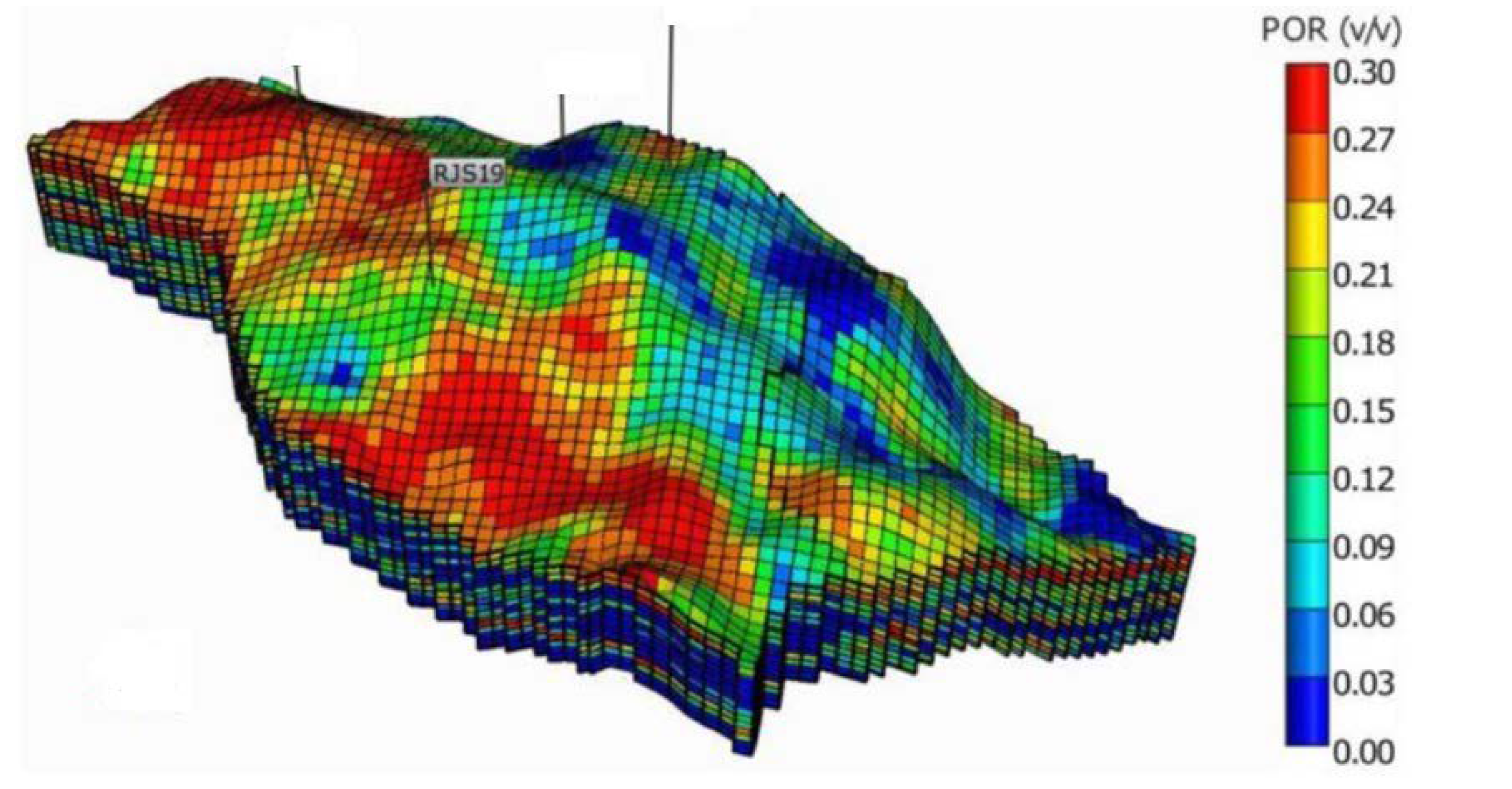
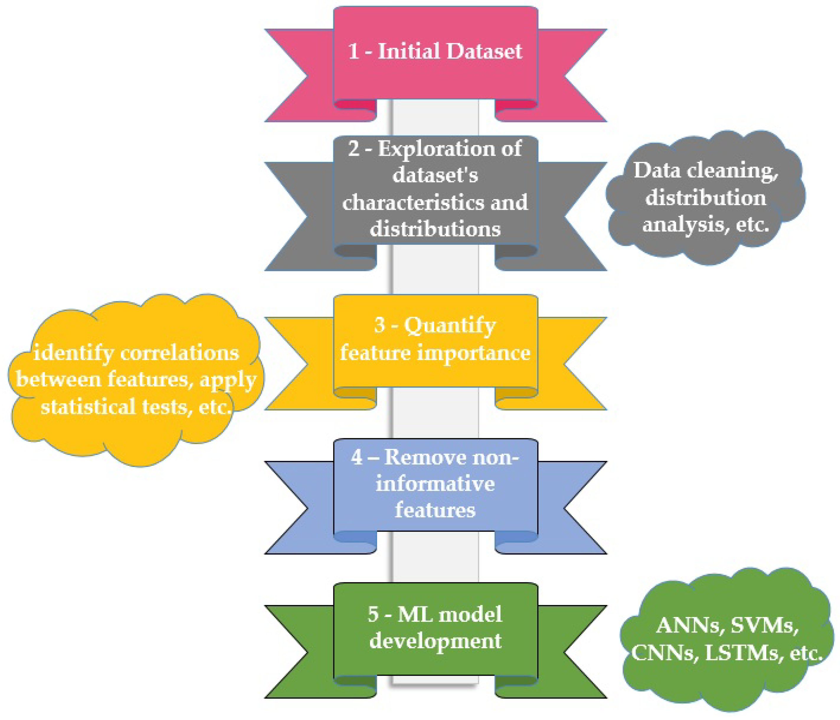
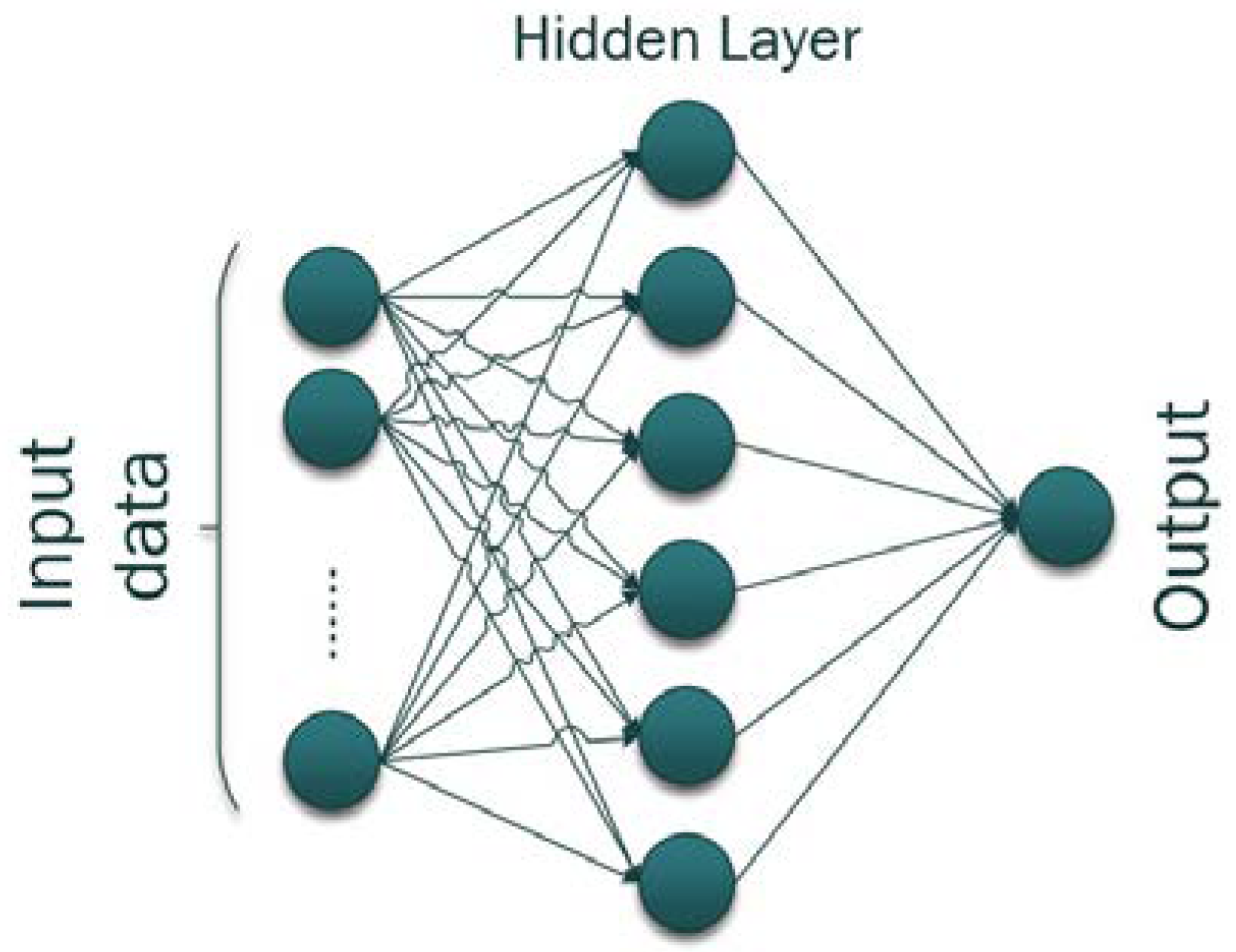
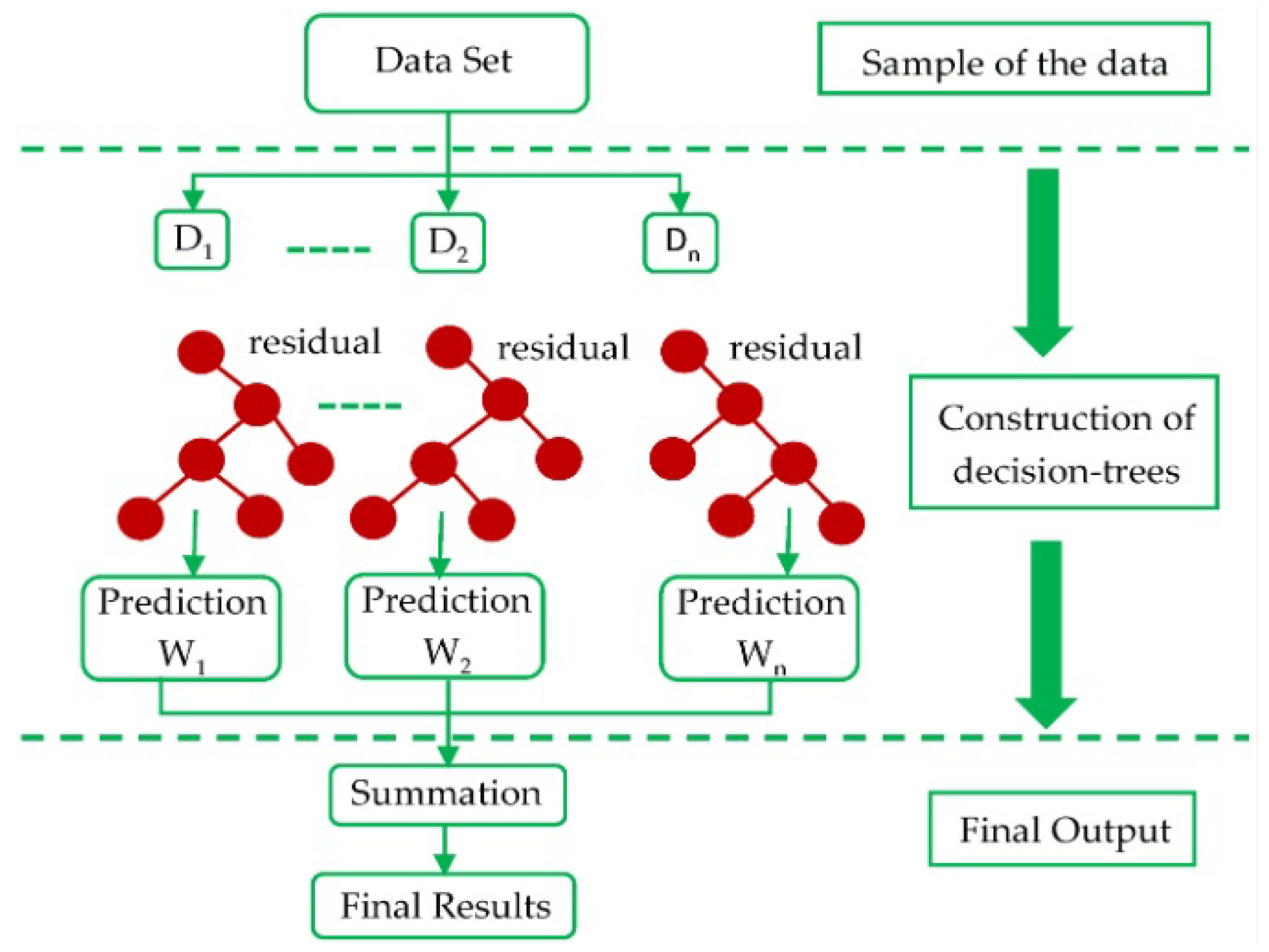
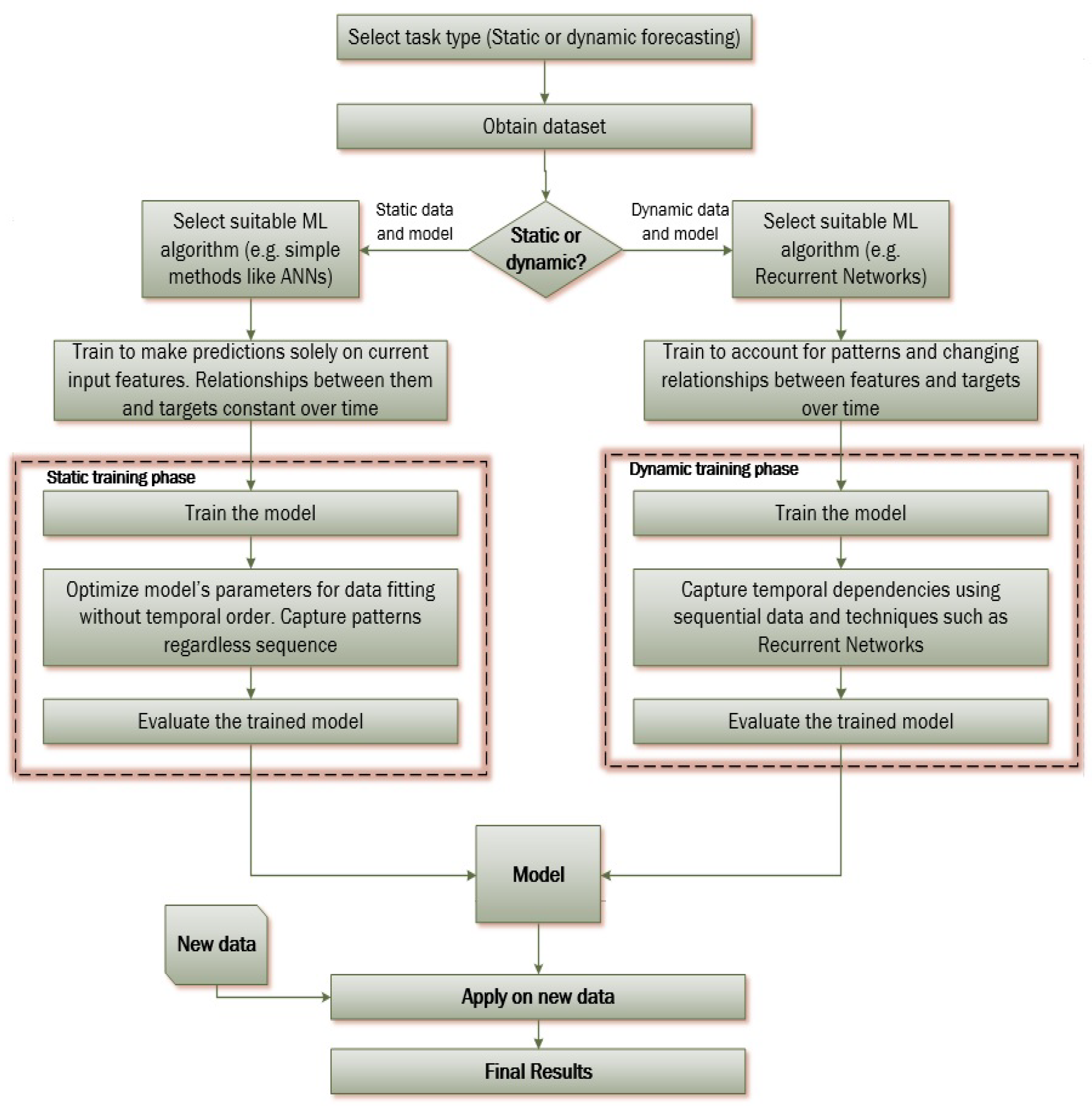
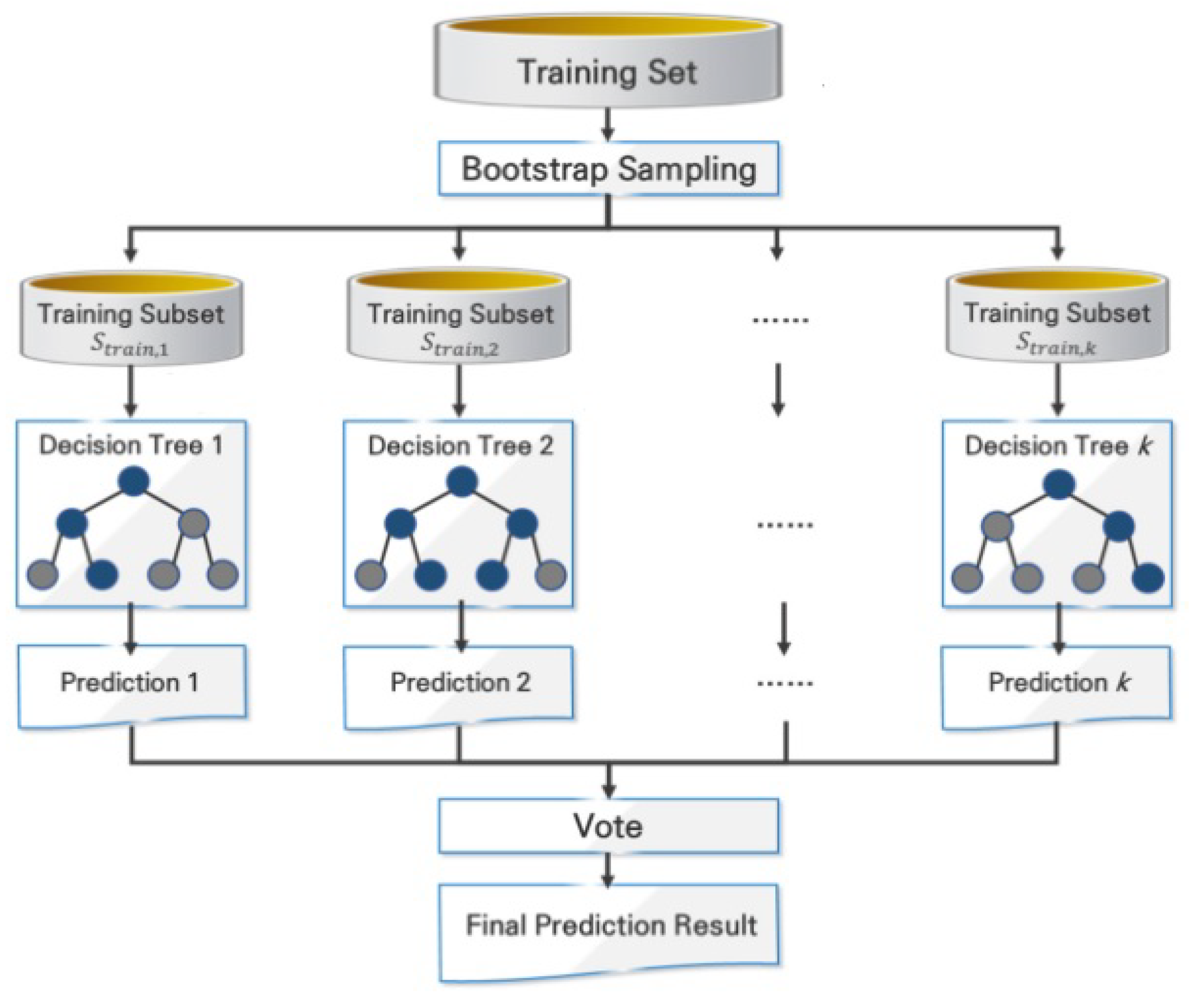
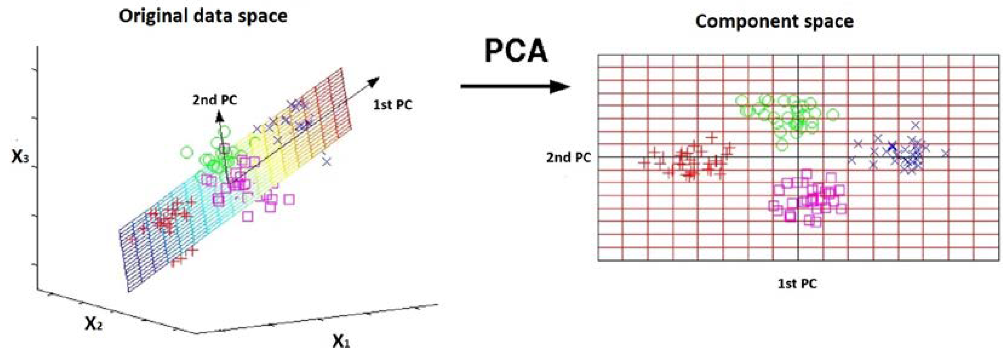
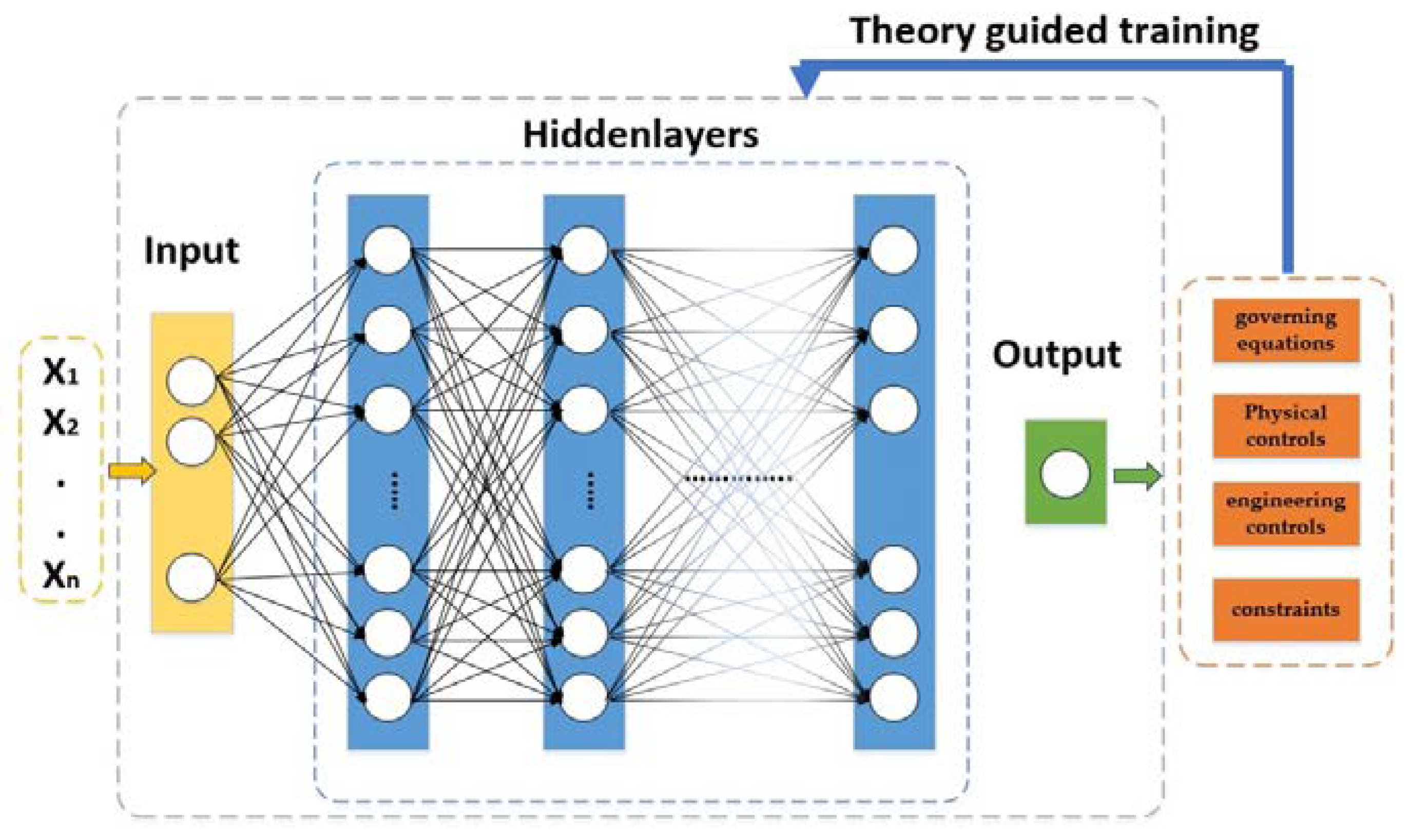
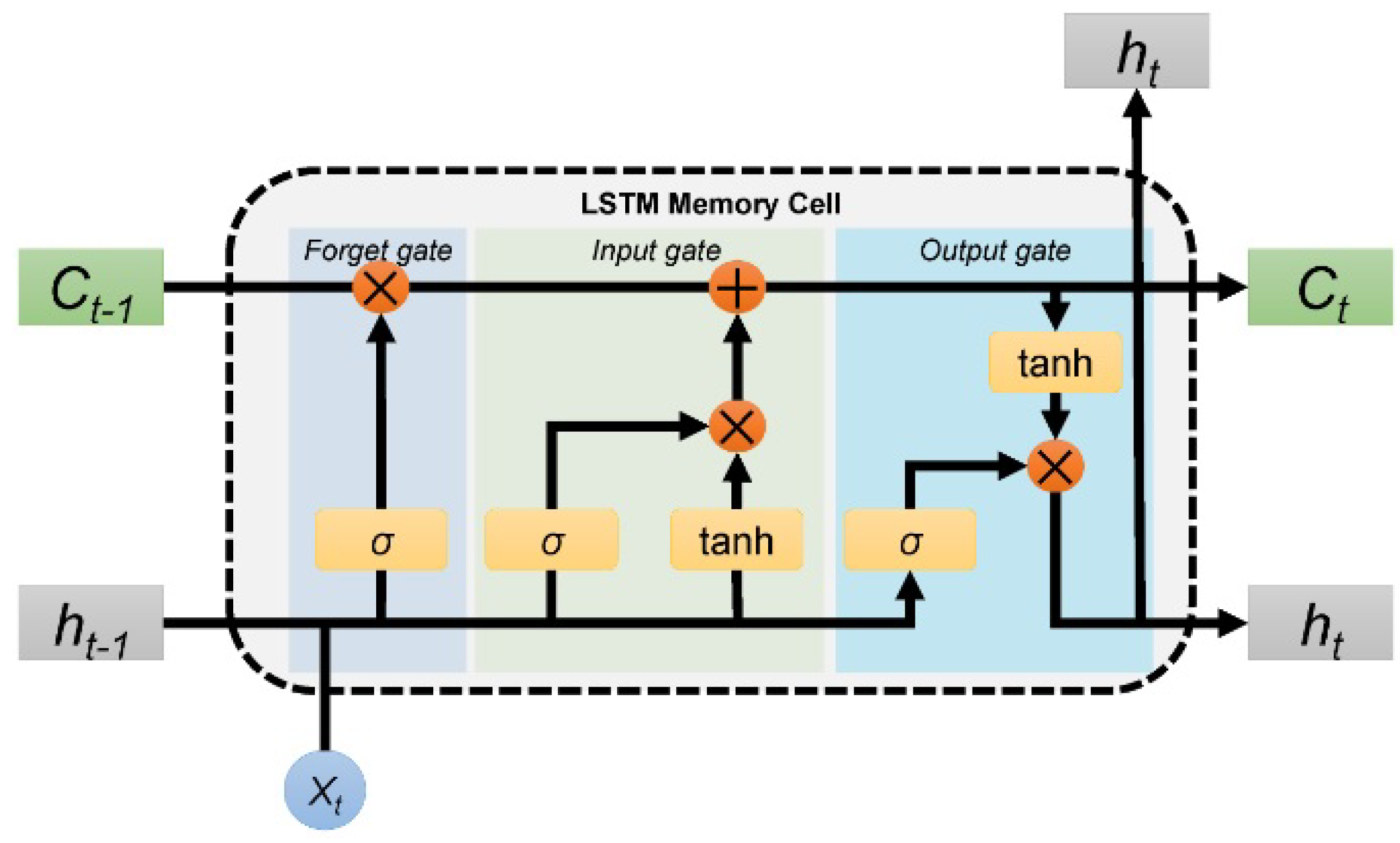
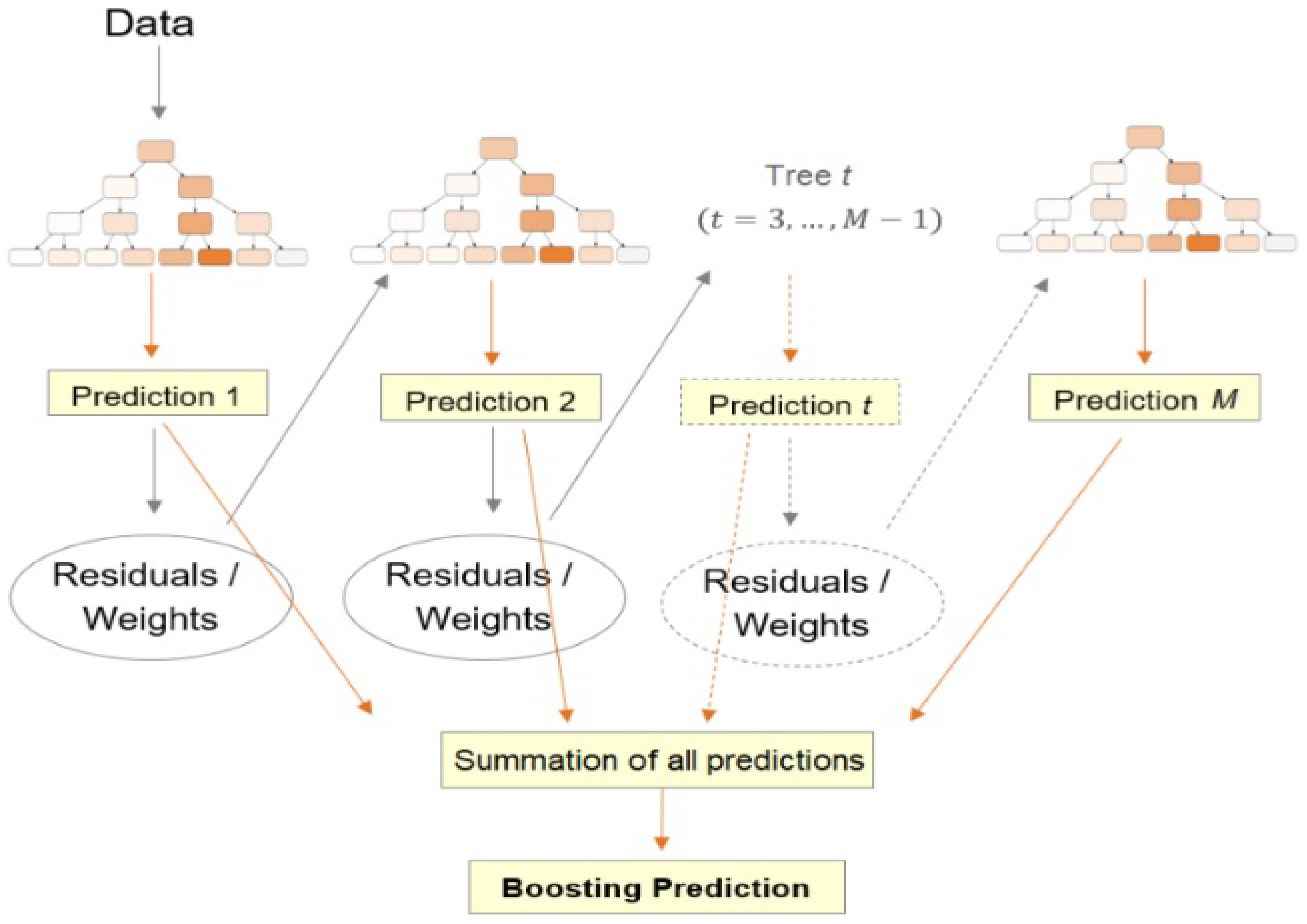
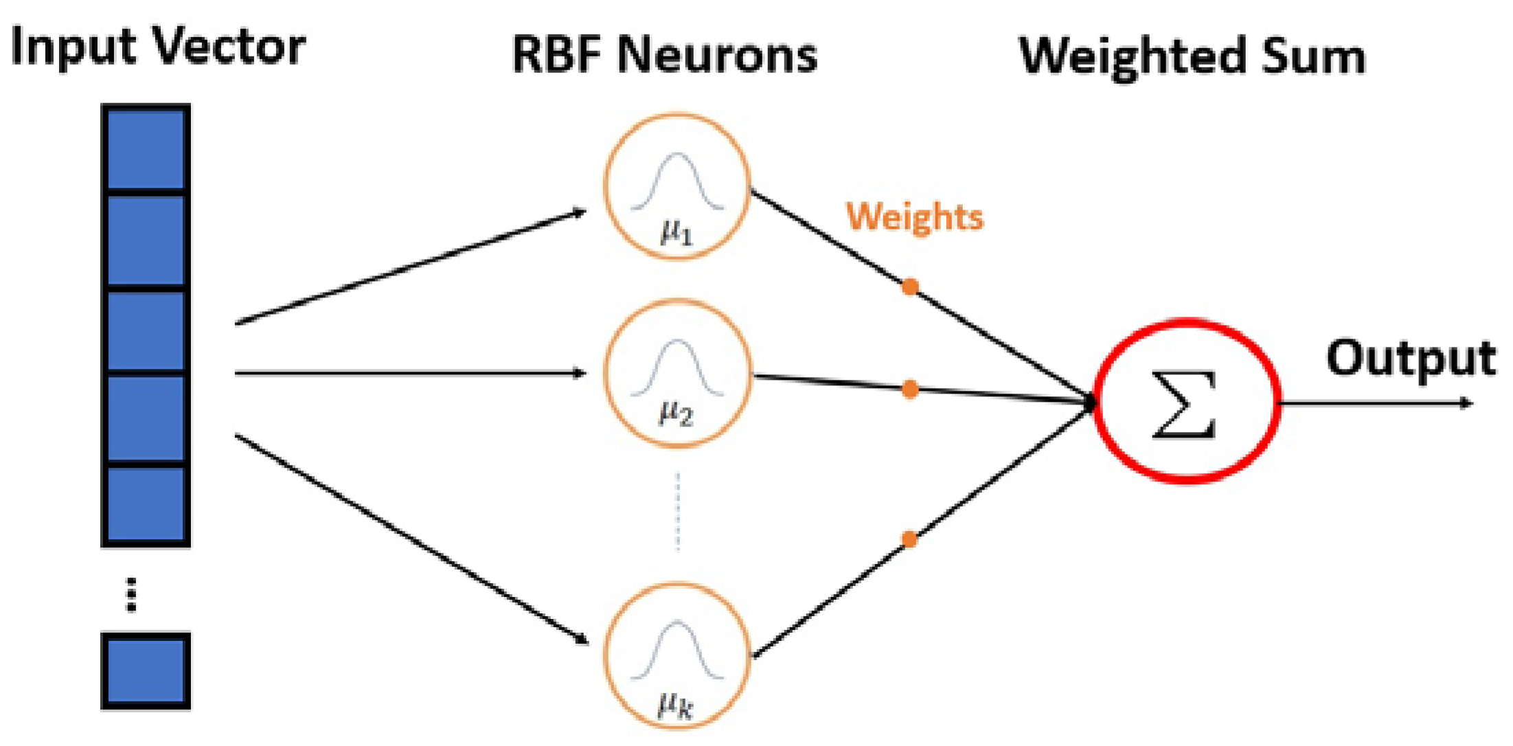
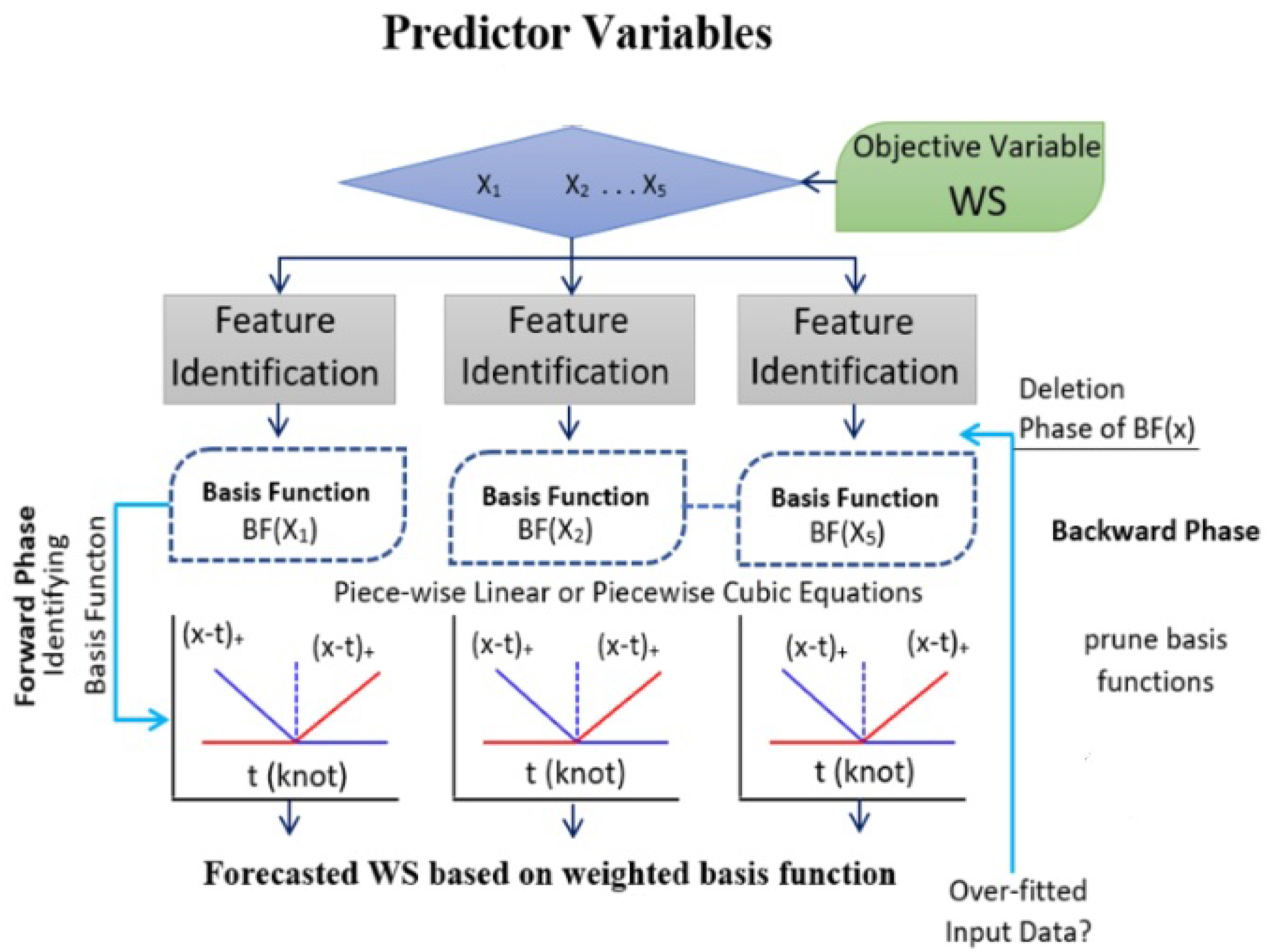
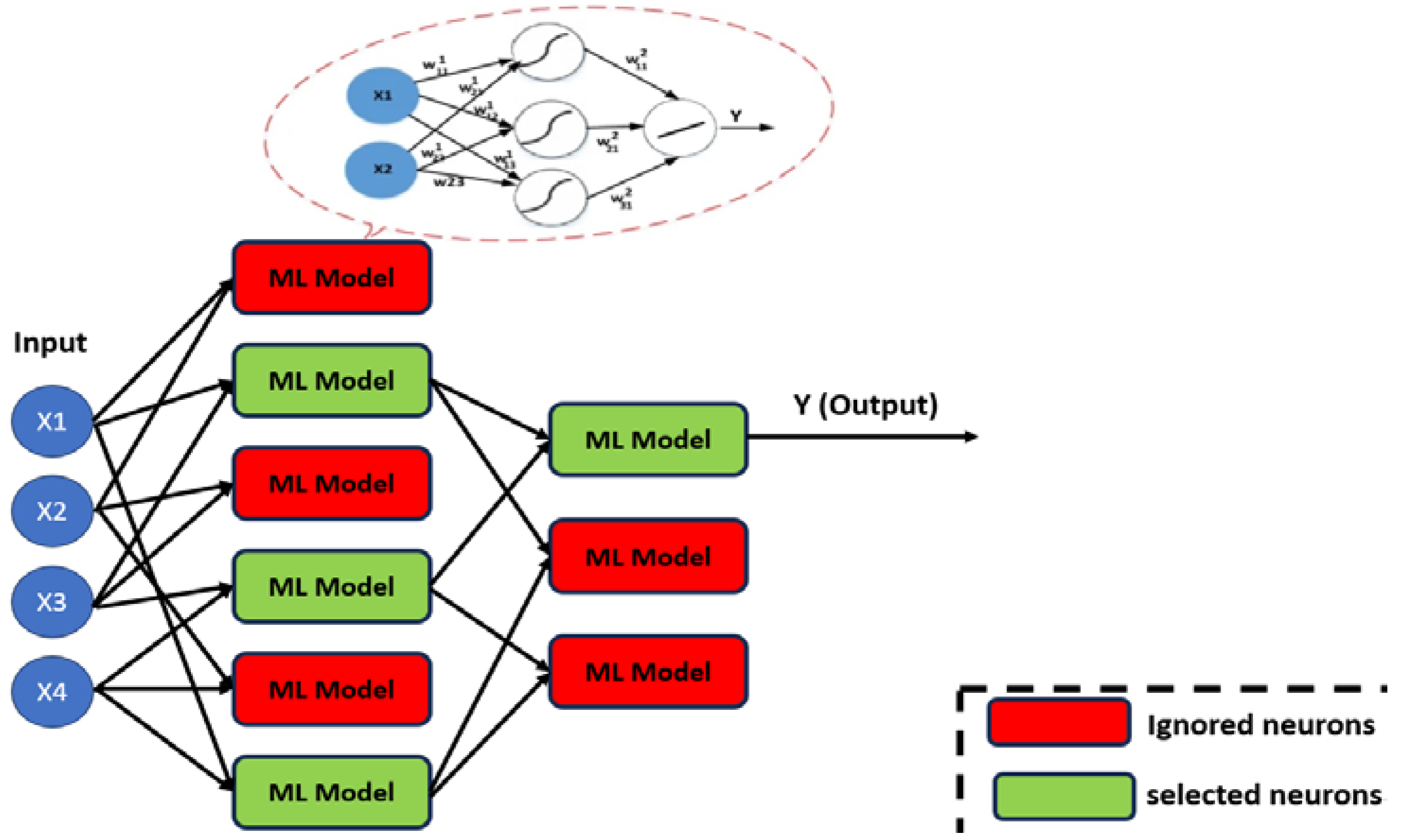
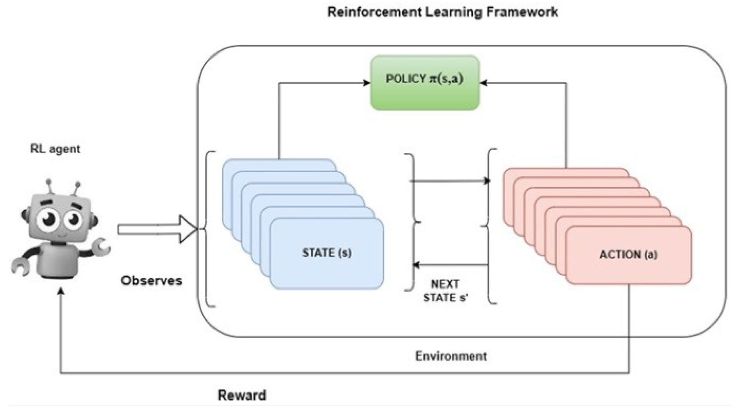
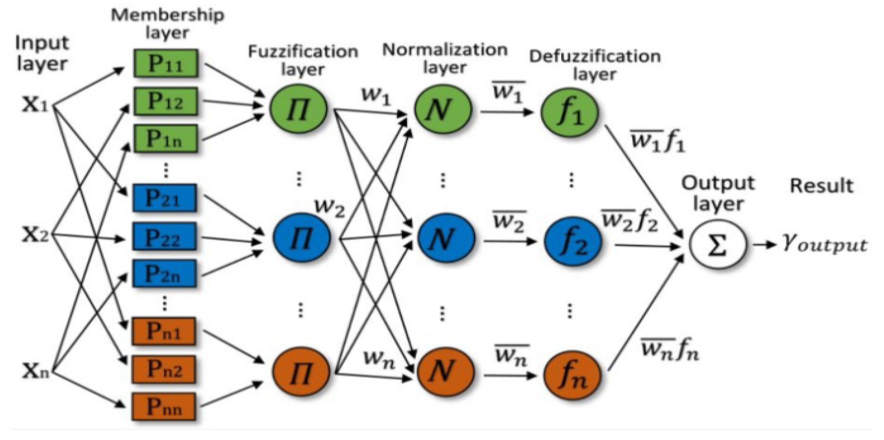
Table 1.
Production forecast and optimization applications summary.
| ML Application | ML Training Scheme | Main Objective | ML Method | Reviewed Studies (Reference List Number) |
|---|---|---|---|---|
| Optimization | Supervised | Production optimization | ANNs or ANNs with optimization techniques | [23,24,25,31,33,93,101] |
| DTs and Ensemble methods (e.g., XGB, GBR, RF) | [33,40,101] | |||
| SVMs and their variations (e.g., LSSVMs, SVRs) | [36] | |||
| Well placement optimization | ANNs or ANNs with optimization techniques | [28,30,92,162] | ||
| DTs and Ensemble methods (e.g., XGB, GBR, RF) | [99] | |||
| Unsupervised | Production optimization | Clustering techniques | [38,39] | |
| Forecasting | Supervised | Static predictions | ANNs or ANNs with optimization techniques | [45,46,48,49,50,51,91,94,100,102,104,113,115,116,117,118,119,120,121,122,123,125,126,127,131,134,140,148,158,159,160,161,163,165,173,174,175,176,177,180,181,189,190,191,192,194,202,210,211] |
| RBFNN | [114,180,199,207] | |||
| DTs and Ensemble methods (e.g., XGB, GBR, RF) | [43,54,96,100,130,133,145,146,147,180,208,210,212] | |||
| SVMs and their variations (e.g., LSSVM, SVRs) | [55,92,100,102,104,110,111,112,133,149,172,179,180,195,196,201,203,205,208,210,211] | |||
| Deep Learning (ANN, encoder- decoder CNN, RNN, etc.) | [56,58,59,60,61,95,132,136,138,139,178,197,198,212] | |||
| Theory guided networks | [63] | |||
| MARS | [129] | |||
| ANFIS | [204] | |||
| GMDH | [142,143,144] | |||
| Unsupervised | GAN | [62,137] | ||
| Reinforcement Learning | Reinforcement algorithm | [167] | ||
| Supervised | Dynamic predictions | RNNs (mostly LSTMs) | [20,44,54,66,71,72,73,75,106,108] | |
| ANNs or ANNs with optimization techniques | [22,76,77,79,86,87,107,135,150,153,169,171,182,183] | |||
| RBFNN | [153,170] | |||
| SVMs and their variations (e.g., LSSVM, SVRs) | [152] | |||
| MTS and VAR | [80] | |||
| HONNs | [84,85] | |||
| Gamma regression | [86,87] | |||
| MLMVN | [89] | |||
| Chaotic Neural Networks | [185] |
Disclaimer/Publisher’s Note: The statements, opinions and data contained in all publications are solely those of the individual author(s) and contributor(s) and not of MDPI and/or the editor(s). MDPI and/or the editor(s) disclaim responsibility for any injury to people or property resulting from any ideas, methods, instructions or products referred to in the content. |
© 2023 by the authors. Licensee MDPI, Basel, Switzerland. This article is an open access article distributed under the terms and conditions of the Creative Commons Attribution (CC BY) license (https://creativecommons.org/licenses/by/4.0/).
Share and Cite
MDPI and ACS Style
Samnioti, A.; Gaganis, V. Applications of Machine Learning in Subsurface Reservoir Simulation—A Review—Part II. Energies 2023, 16, 6727. https://0-doi-org.brum.beds.ac.uk/10.3390/en16186727
AMA Style
Samnioti A, Gaganis V. Applications of Machine Learning in Subsurface Reservoir Simulation—A Review—Part II. Energies. 2023; 16(18):6727. https://0-doi-org.brum.beds.ac.uk/10.3390/en16186727
Chicago/Turabian StyleSamnioti, Anna, and Vassilis Gaganis. 2023. "Applications of Machine Learning in Subsurface Reservoir Simulation—A Review—Part II" Energies 16, no. 18: 6727. https://0-doi-org.brum.beds.ac.uk/10.3390/en16186727
Note that from the first issue of 2016, this journal uses article numbers instead of page numbers. See further details here.