
Applications of Machine Learning in Subsurface Reservoir Simulation—A Review—Part I

1
School of Mining and Metallurgical Engineering, National Technical University of Athens, 15780 Athens, Greece
2
Institute of Geoenergy, Foundation for Research and Technology-Hellas, 73100 Chania, Greece
*
Author to whom correspondence should be addressed.
Energies 2023, 16(16), 6079; https://0-doi-org.brum.beds.ac.uk/10.3390/en16166079
Submission received: 8 July 2023
/
Revised: 4 August 2023
/
Accepted: 17 August 2023
/
Published: 20 August 2023
(This article belongs to the Special Issue Artificial Intelligence/Machine Learning Applications in the Oil and Gas Industry)
Abstract
:In recent years, machine learning (ML) has become a buzzword in the petroleum industry with numerous applications that guide engineers toward better decision making. The most powerful tool that most production development decisions rely on is reservoir simulation with applications in numerous modeling procedures, such as individual simulation runs, history matching and production forecast and optimization. However, all these applications lead to considerable computational time- and resource-associated costs, and rendering reservoir simulators is not fast or robust, thus introducing the need for more time-efficient and smart tools like ML models which can adapt and provide fast and competent results that mimic simulators’ performance within an acceptable error margin. The first part of the present study (Part I) offers a detailed review of ML techniques in the petroleum industry, specifically in subsurface reservoir simulation, for cases of individual simulation runs and history matching, whereas ML-based production forecast and optimization applications are presented in Part II. This review can assist engineers as a complete source for applied ML techniques since, with the generation of large-scale data in everyday activities, ML is becoming a necessity for future and more efficient applications.
1. Introduction
1.1. Reservoir Simulation in the Oil and Gas Industry
The discovery of oil and gas reserves and their exploitation to provide access to affordable energy, meet the world’s energy demand and maximize profit are the main objectives of the petroleum industry and its applications. Subsurface reservoir simulation is currently the most essential tool available to reservoir engineers for achieving those goals. It is crucial for the deep understanding and detailed analysis of a reservoir’s behavior as a whole, as well as for designing and optimizing recovery processes. Simulation is utilized in all essential planning stages, for reservoir development and management purposes, to make the exploitation of underground hydrocarbon reservoirs as efficient as possible.
Reservoir simulation is developed by combining principles from physics, mathematics, reservoir engineering, geoscience and computer programming to model hydrocarbon reservoir performance under various operating strategies, according to each reservoir’s respective characteristics and production conditions. A reservoir simulator’s output, typically comprised of spatial and temporal distributions of pressure and phase saturation, is introduced to simulation models of physical components in the hydrocarbon production chain, including those used to produce fluids at the surface (wellbore) and process the reservoir fluids (surface facilities), thus allowing for a complete modeling system down to the sales point [1,2]. Reservoir simulations are mathematical tools built to accurately predict all the physical fluid flow phenomena inside a reservoir within a reasonable error margin, thus acting as a “digital twin” of the physical system.
Simulators estimate a reservoir’s performance by solving the differential and algebraic equations derived from the integration of mass, momentum and energy conservation together with thermodynamic equilibrium, which describe the multiphase fluid flow in porous media. By using numerical methods, typically finite volumes, these equations can be solved throughout the entire reservoir model for variables with space- and time-dependent characteristics, such as pressure, temperature, fluid saturation, etc., which are representative of the performance of a reservoir [2].
For this task, a static and a dynamic reservoir model must first be set up. A static reservoir model is a three-dimensional representation of a reservoir’s geological properties, such as porosity, permeability and rock type. It is created using geological, well and seismic data together with a thorough interpretation, providing an approximate ‘’snapshot’’ of a real reservoir at a specific time [3,4,5]. On the other hand, a dynamic reservoir model is a time-dependent simulation of fluid flow in a reservoir. It builds upon the static model by incorporating production history, fluid properties and reservoir management strategies. A dynamic model is employed to predict reservoir behavior, optimize production and assess various development scenarios, such as enhanced oil recovery techniques and the impact of drilling new wells.
When both static and dynamic reservoir models have been created, they are integrated to estimate the reservoir’s performance. The simulator then divides the reservoir into many cells (grid blocks) or otherwise into a large number of space and time sections, where each cell is modeled individually (Figure 1). The simulation method assumes that each reservoir cell behaves like a tank with uniform pressure, temperature and composition of the individual phases for each specific time. During the fluid flow, each cell communicates with all neighboring cells to exchange mass and energy. Subsurface reservoir models can be highly complex, exhibiting high inhomogeneity, a vast variance of petrophysical properties, such as porosity and permeability, and peculiar shapes capturing the structure and stratigraphy of the real reservoir.
Typically, the simulation of the thermodynamic behavior of fluids in reservoirs is handled by means of black oil or compositional fluid models. Black oil models are widely used to express simple phase behavior phenomena, especially for low- to medium-volatility oils [6], providing a simple and sufficiently precise approach. These models utilize the black oil assumption for which the fluid, at any point along the flow inside the reservoir to the surface facilities, is considered as a binary composition fluid consisting of the stock tank oil and the surface gas. Consequently, at any given pressure, the stock tank oil is saturated with a quantity of tank gas that induces its swelling and if a further quantity of gas is present, it coexists with the oil as a free gas phase. The change in the volume of water with pressure can also be considered whereas any phase-related changes are ignored since water is assumed not to interact with hydrocarbons in such a way. These phase behavior phenomena are quantified using PVT properties that are only functions of pressure and temperature, hence ignoring the influence of the exact fluid composition [7].
When complex phase behavior phenomena take place, such as in the case of CO2 injection into a reservoir for enhanced oil recovery (EOR) purposes, the black oil assumption is no longer valid. Thus, fully compositional simulations need to be utilized to monitor in detail the fluid composition’s changes at each block and at each time step [8]. In compositional reservoir simulation, phase behavior calculations needed for each grid block of the reservoir are conducted by running stability and flash calculations based on an equation of state (EoS) model. Stability provides the number of fluid phases present in the cell (typically oil, gas or both) whereas flash calculations provide the amount and composition of all phases in equilibrium. These computations normally account for a significant part of the total CPU time and, as a result, compositional simulations need high-performance systems with significant computing power to be executed successfully [9,10]. Depending on the number of components used to describe the fluids, there is a very high demand for computational power due to the complexity and the iterative nature of the phase behavior problem solution process. Phase stability and phase split computations often consume more than 50% of the simulation’s total CPU time, as both problems need to be solved repeatedly for each discretization block at each iteration of the non-linear solver and for each time step [10]. The reservoir model configuration is completed by adding the reservoir–rock interaction, typically in the form of relative permeability and capillary pressure curves, as well as information on the producing/injecting wells, their perforations and their operating schedule.
Once the reservoir model has been set up, the most fundamental and, at the same time, computationally expensive applications of compositional simulation are reservoir adaptation, known as history matching (HM), and production forecast and optimization (PFO) of future reservoir performance. HM is the most important step preceding the calculations for the optimization of reservoir performance. It is the process of calibrating the uncertain properties and parameters of a reservoir model (such as petrophysics), based on a trial-and-error procedure, until the production and pressure values predicted by the field’s dynamic model match the historically recorded ones. Therefore, HM is an optimization problem since the Objective Function (OF) that must be minimized accounts for the difference between the data derived from the simulator and the measurements obtained from the field. Once completed, the reservoir model can be considered reliable enough to be used to perform all desired engineering and economic calculations, predictions, and production optimization [11].
Prediction of reservoir performance under various production scenarios and its optimization is the next most crucial application of reservoir simulation since production management and techno/economic planning are highly dependent on it. The primary use of reservoir performance prediction is focused on estimating the oil recovery under various production schemes, designing the wells’ configuration based on those strategies and conducting economic analysis for the future development of fields so that strategic decisions and economic evaluations are properly justified [12].
Although the above two applications are considered the core of reservoir engineering, they suffer from extremely large computational expenses due to the iterative nature of the calculations needed for their proper execution. They can be very cumbersome for very extensive and detailed reservoir models since the increasing number of grid blocks, the variant distribution of the reservoir parameters and the complexity of the wells’ operation schedule increase the time required for the calculations of a conventional non-linear solver [11]. Therefore, speeding up these applications is of great importance and each one must be considered as a separate subject for optimization.
Reservoir simulators have been modernized to meet the current needs of large data management by incorporating recent developments in High-Performance Computing (HPC), including the use of multi-threading, multi-core, multi-computer grids and cloud computing [13]. However, the continuous growth of the models’ size, resolution and physics complexity renders simulators not as fast or robust enough, thus introducing the need for more time-efficient and smart computational tools like proxy models which can adapt and provide fast and competent results that mimic real reservoir performance within an acceptable error margin.
Proxy reservoir models, also known as Surrogate Reservoir Models (SRMs), behave as the “digital twin” of a conventional reservoir simulator, in the sense that they aim to mimic its results by identifying and modeling the underlying complex relationships between various input variables and the desired outcome (i.e., pressure and saturation), in a very small fraction of the time that would otherwise be required. Proxy modeling can be broadly classified into four categories, based on their development approach, namely statistics-based models, Reduced Physics Models (RFMs), Reduced Order Models (ROMs), and Artificial Intelligence (AI)-based models, like machine learning (ML). Statistics-based models (e.g., response surfaces) provide a function that approximates the response of a full numeric simulator by capturing the input–output relationship of a sample of input parameters [14]. RFMs aim at simplifying the physics of a process, in this case, the fluid flow process inside the reservoir, by applying several hypotheses, while ROMs are used to decrease a primary system’s dimensionality by ignoring insignificant parameters while, at the same time, keeping the dominant features and physics over a defined space [14,15]. In the present review, ML-based models are considered in detail thanks to their ability to identify trends and patterns between input variables and the desired outcome and of handling multi-dimensional and multi-variety data.
1.2. Machine Learning in Reservoir Simulation
Learning from data has been a rich topic of research in many engineering disciplines since the volume of data has increased greatly and human cognition is no longer able to decipher the information and find patterns within associated data [16]. In recent years, data-driven ML techniques have gained major support and have been applied successfully to assist in field development plans. They allow the development of models that represent physical problems without the demand to mathematically express first-principle laws. Typically, they consist of a function or a differential equation that estimates the output of conventional full-scale reservoir simulation models [17,18,19], producing approximate and partially imprecise results to give fast, robust and low-cost solutions by sacrificing some accuracy for gains in agility and acceleration [19].
ML provides an automated approach to the development of numerical models that learn to recognize patterns from observed data and facilitate the decision-making process with minimal human interference. The most common types of ML are supervised learning (SL), unsupervised learning (UL) and reinforcement learning (RL), as presented in Figure 2. SL models focus on identifying the underlying relationship between observed data (inputs) and the corresponding observed outcome (output) and build a mathematical model to express their relationship. This way, when new input data arrive, the model can provide predictions of the output as efficiently as possible. They are used to solve classification and regression problems depending on whether the required output is a discrete variable (i.e., a class number) or a continuous one. UL is used when the observed data are unlabeled (i.e., there is no corresponding output) and its main purpose is to identify hidden patterns only between the given input data. Such models are mostly used for data clustering, which is a method for data partitioning into groups based on similarities with each other. RL is a method, lying in the system control context, that is based on generating models, known as agents, that predict appropriate actions, based on the observed data, to reward desired outcomes and/or punish undesired ones. As in UL, the observed data are unlabeled and, thus, the RL algorithm must instead try to first explore its environment and then determine the output which maximizes a reward through a trial-and-error process [20].
SL models can be used for classification and regression problems. In cases where the output is a continuous numerical value, the problem can be solved using regression algorithms, whereas if the output is a qualitative/discrete label, the problem is handled with classification models. Classification assigns a given observation to several discrete categories, called labels or classes, and is mostly used for pattern recognition and class predictions [20]. In their elementary form, binary classification problems assign classes to the input data, such as yes/no, 0/1, etc., although multiclass problems can be handled as well. During their training, classifiers learn each class’s decision boundary using ML algorithms that try to minimize the misclassification error [21]. Typical examples of regression modeling are models predicting fluid properties given field measurements. Similarly, classifiers can be used to identify whether a fluid is in its vapor, liquid or supercritical state based on its composition and prevailing conditions.
An ML model’s development is completed in three main steps. The first step is data gathering to form a sufficiently large dataset, which is of utmost importance since the quantity of data directly affects the accuracy of the model. This dataset, called the training dataset, is later used for the model’s training process. The second step is data preparation, or else data pre-processing, such as dimensionality reduction, outliers and missing data detection, etc. This step is crucial since the model’s prediction precision depends also on the data quality, along with quantity. Finally, the last step is the model’s training, using the training dataset, which consists of the input variables as well as the desired output (for SL). The latter is represented by a class number for the classification and by a numeric value for the regression model. It must be noted that both regression and classification models should be assessed based on their ability to predict and classify, respectively, a blind dataset (i.e., previously “unseen” data) that has not been incorporated in the original training dataset. That way, a model’s generalization capability can be evaluated and optimized to avoid creating overtrained models, which, although they provide very good results for a specific training dataset, provide poor accuracy for a new “unseen” one (overfitting) [22,23].
In the subsurface reservoir simulation context, as shown in Figure 3, conventional simulators are utilized to generate large ensembles of data offline, for various operating conditions, which are then used to train an ML model. It is crucial to note that, unlike most ML applications, the derived data are usually obtained by a computational process (i.e., the offline simulation runs) rather than some experimental procedure; hence, it is noiseless. After the model has been trained using the noiseless calculated data, it acts as the reservoir’s ‘’digital twin’’ which can now provide fast and accurate predictions about the reservoir’s past, ongoing and future performance that a classic industry simulator would need a large amount of time to perform. That way, the model can be applied to address various problems and effectively support the decision-making process more expediently.
Τhe era of ML as a fitting technique emerged back in the early 1990s by researchers who fully introduced the concept of ML, more specifically Artificial Neural Networks (ANNs), like Freeman and Skapura [24], Fauset [25] and Veelenturf [26]. However, since then, there have been numerous endeavors to apply ML in the oil and gas industry. These efforts aim to develop intelligent AI systems as an alternative to traditional reservoir simulation calculations. The number of offered ML-based solutions to engineering problems has significantly increased, as evidenced by the successful implementation of several methods for a variety of petroleum engineering problems, such as exploration [27,28], drilling operations [29,30], PVT behavior [31], reservoir management and field development planning [32], facilities monitoring and inspections [33] and, recently, chatbots [34], which guide engineers through the process of archive digging, suggest solutions to problems, etc.
While ML has shown promise in reservoir simulation applications, it also has some limitations that must be considered. The first limitation concerns data availability and quality since ML models heavily rely on large volumes of high-quality data for their effective training and performance. Nevertheless, in most of the reservoir simulation ML applications, the data used in the training process of a ML model are obtained by running conventional simulations offline; hence, the obtained data can be arbitrarily large and noise-free.
Many ML algorithms are often considered as “black box” models, meaning it can be difficult to interpret and understand the reasoning behind their predictions. This lack of interpretability can be a limitation in reservoir simulation, where engineers may require insights into the underlying physics and mechanisms driving the system behavior. In addition, ML models are usually trained on historical and/or observed data and, while they can provide accurate predictions for scenarios similar to those they have been trained against, they may struggle to generalize well to unseen or significantly differing conditions. Reservoir systems are complex and can exhibit unique characteristics, making it challenging for ML models to handle novel or rare situations.
A major aspect is the fact that ML models may not readily incorporate prior knowledge or physical laws specific to reservoir engineering. Integrating domain knowledge into ML models is crucial for maintaining physical consistency and ensuring realistic simulation results. It is of utmost importance to be aware of these limitations when applying ML in reservoir simulation. Careful consideration, appropriate data handling and model validation can help mitigate these limitations and make the best use of ML in reservoir simulation applications.
This review discusses the approaches of ML-based reservoir simulations to provide a wide perspective on the state-of-the-art methods currently in use for individual simulation runs and HM. It must be noted that the ML methods for PFO applications are reviewed in the second part (Part II) of the present review series due to the excessively large number of approaches that have been proposed on this subject.
The main goal of the first category which is based on individual simulation runs is to build ML models that reduce the overall simulation runtime by rapidly determining cell-specific parameters. Typical examples of proxy models include predicting the prevailing pressure and saturation, effectively replacing the need for a non-linear solver, and predicting the prevailing k-values, enhancing the efficiency of complex and iterative phase behavior calculations. Subsequently, the rapidly responding proxies can be introduced to any desired HM or PFO calculation, thus accelerating those tasks by orders of magnitude. The second category of HM, as a computationally expensive process, can benefit largely from the generation of proxy models that aim to optimally calibrate the uncertain parameters to achieve a good match between calculated and observed production data.
The great physical size and lack of homogeneity of hydrocarbon reservoir models require numerical models comprising a large number of cells, thus in turn imposing the need for ML-based accelerating techniques in all calculations involved such as individual runs, history matching and production optimization. However, hydrocarbons are not the only fossil fuel requiring advanced modeling techniques. For example, multiple-seam coal mining also poses a huge load due to the complexity of the 3D finite element (rather than finite volumes) method commonly used to simulate their performance.
The current process of mineral exploration can generate an enormous amount of data in the form of soil samples, geochemistry, drill results, test results, etc. Therefore, ML is employed to aid in numerous complex mining operations, such as identifying potentially promising mining areas, accelerating exploration, productivity improvement, environmental monitoring, predictive maintenance and much more.
Although the oil and gas industry, the coal mine industry and other energy sectors exhibit major differences in terms of production and operations, drawing parallels between the use of ML methods in those industries is important for several reasons. Firstly, by comparing how ML techniques have been successfully applied in different energy sectors, knowledge and best practices can be shared and transferred. What works well in one industry may inspire solutions or improvements in another, leading to more efficient applications. Furthermore, although the specific domain expertise and datasets may differ between industries, there are likely shared ML applications. For instance, problems related to predictive maintenance, improvement of technological schemes and mining-geomechanical models [35], operations and emission numerical simulations [36], productivity and safety [37] and finite element computer modeling [38] have similar underlying principles within the oil and gas industry. Thus, lessons learned in one industry can be applied to another. Finally, regardless of the specific sector, the energy industry faces similar societal and environmental challenges. Leveraging ML across different industries can collectively address energy efficiency, emissions reduction and sustainable resource management.
The major objective of the present review paper on ML applications in reservoir simulation is to provide a comprehensive overview of the recent, older and state-of-the-art ML techniques and methodologies applied in reservoir simulation. This involves discussing various ML algorithms, data preprocessing techniques, model training and evaluation approaches and their specific applications in reservoir simulation. Furthermore, this review also evaluates their performance and effectiveness in reservoir simulation and discusses the strengths, limitations and applicability of various ML algorithms in addressing different reservoir engineering problems. By pursuing these objectives, the current review on ML applications in reservoir simulation seeks to offer a comprehensive and informative reference for researchers, practitioners and decision makers operating on such tasks within the oil and gas industry.
In this paper, the ML methods for subsurface reservoir simulation reviewed are categorized based on the context of the problem under investigation and the ultimate purpose of each reviewed method. Section 2 describes generic proxy methods, like predicting the k-values, which can be utilized to speed up any desired reservoir simulation application whereas Section 3 reviews methods that directly serve the HM. Section 4 concludes the present review.
2. Machine Learning Strategies for Individual Simulation Runs
Reservoir simulation software packages are continuously being modernized based on the current needs for large data management and despite the availability of ever-growing computer power. However, simulations are still not fast or robust enough, in the context that they entail high computational costs, introducing the need for more time-efficient smart tools that can adapt and provide fast and competent predictions which mimic real reservoir performance within an acceptable error margin. In this section, ML is employed as a suitable means to accelerate individual simulation runs that can assist any desired HM or production-related calculations by using two approaches.
Firstly, fast proxy models (or else SRMs) of reservoir simulators have been proposed and can be implemented to answer a wide range of engineering questions in a fraction of the time that it would otherwise be required. Secondly, ML has been utilized to accelerate specific CPU time-intense sub-problems while maintaining the rigorous differential equation-solving method. The most pronounced application in this category is the handling of the phase equilibrium problem in its black oil or compositional form which needs to be solved numerous times during reservoir simulation runs.
SRMs using ML and pattern recognition methods to fully replace the non-linear solver were first proposed by Mohaghegh and his associates who developed SRMs that could fully reproduce the traditional black oil or compositional reservoir simulation results (i.e., high-fidelity models) on a cell basis without sacrificing the physics or the order of the system under investigation, as is the case of RFM and ROM methods, respectively. Instead, they built grid-based and well-based proxy models. Grid-based models usually provide pressure and saturation predictions for the fluid phases at the grid level based on information from the surrounding grid blocks rather than the whole reservoir. This way, the very weak dependency of the state of a cell on the ones far away from it is ignored while allowing at the same time the disengagement of the cell state. Well-based models are developed similarly to predict well-related parameters, such as gas, oil and/or water production rates, Bottom Hole Pressures (BHPs), etc.
The second category is based on rapidly and accurately predicting fluid properties, both for compositional and black oil models. As already mentioned in Section 1, compositional models are developed to monitor the fluid composition’s changes at each grid block and at each time step. Therefore, the phase behavior calculations needed for each grid block are conducted by running stability and flash calculations, processes that normally take a significant part of the total CPU time. The most burdensome fluid parameter involved in these calculations is the equilibrium coefficients, known as k-values. Their estimation is based on complicated numerical calculations, utilizing EoS-based fluid thermodynamic models, which require a large number of iterations to converge; simultaneously, they need to be performed for all grid blocks at each time step and each iteration of the non-linear solver. Thus, it is made clear that a regression-based ML model that is capable of directly predicting the necessary k-values and replacing the conventional iterative approach can significantly accelerate any simulation process [22].
Apart from predicting the k-values, another efficient way to reduce the overall computational cost is to recast the phase stability problem to a classification one, using classification ML methods, with two labels corresponding to stable/unstable fluid mixtures or single/two-phase flow. It is important to note that the execution of a phase split calculation is dependent on the stability problem. When stability tests are conducted and instability is detected, it triggers the initiation of a phase split calculation. In this kind of classification problem, the input consists of fluid composition, pressure and temperature values for the classifier to reach a solution (stable or unstable mixture) based on the phase boundaries of the p–T phase diagrams. That way, the trained classifier can replace the traditional iterative stability algorithm and substantially accelerate flow simulations with its direct non-iterative predictions [39].
For the case of black oil simulations, the grid blocks are assumed to contain three primary fluid phases (oil, gas, water). The PVT properties needed to account for the compressibility of each phase (oil, gas and water formation volume factors: Bo, Bg and Bw, respectively), the ratio of gas to reservoir oil (Gas-to-Oil Ratio—GOR) and saturation conditions (bubble and dew point pressure) which are usually readily available from experimental procedures are introduced into the simulator to perform the desired calculations. If experimental values are not available, empirical correlations are used to predict the fluids’ PVT properties utilizing field data (API, gas specific gravity and GOR). However, these correlations are not always accurate since they only perform well for the range of compositions and conditions against which they were generated, thus exhibiting poor behavior outside these bounds. As a result, to speed up and improve the accuracy of the simulation process, ML-based models have been developed, predicting these crucial parameters [40].
2.1. Machine Learning Methods for Surrogate Models
The first attempt to develop a fast proxy of a subsurface reservoir simulator was accomplished by Mohaghegh and his associates, who ran numerous studies and set up SRM methodologies by utilizing intelligent system techniques to approximate the simulation process of huge complex oil fields which would otherwise require an extremely large amount of CPU time. SRMs can mimic the behavior of a full reservoir model with precision, can be used in many applications (i.e., PFO and HM) and, in some cases, they can fully replace numerical simulators or work with them in a coupled way. This group developed many workflows, usually using ANNs, in which they propose the detailed development of such models, such as fracture propagation inverse problems, to identify potential hydraulic fracture designs [41], uncertainty analysis [42,43,44,45,46], prediction of dynamic reservoir properties [1], waterflooding operations [47], CO2 EOR and storage projects [48,49], etc. Results show that the SRMs are capable of efficiently mimicking the simulator’s predictions with fewer runs, compared to the conventional reservoir simulator that needs an excessive number of simulations, especially for complex fields.
Dahaghi et al. [50] proposed a similar methodology to obtain cumulative production predictions, this time for a complex fractured shale gas reservoir. They used ML and data mining methods to create a single-well shale SRM model to deal with direct (e.g., production prediction) as well as inverse problems (e.g., HM). According to the authors, the model was characterized as being of great efficiency and it successfully mimicked the conventional simulator with great accuracy and speed. The proposed model can be utilized for HM, uncertainty quantification and real-time production optimization. Memon et al. [51] tried a similar method by building a well-based Radial Basis Function Neural Network (RBFNN) SRM based on black oil simulation results for an initially under-saturated reservoir to predict the flowing BHP. The model’s input parameters consisted of a spatiotemporal dataset (e.g., porosity, permeability, initial oil and water saturation and oil rate). The proposed model was very efficient in comparison with conventional simulators and it can be used for many production optimization purposes by generating hundreds of accurate runs in a fraction of time that would otherwise be needed. Amini et al. [14,52] generated an SRM using ANNs to approximate the CO2 and pressure distributions for a CO2 sequestration process in a depleted reservoir. The authors ran several scenarios using a conventional simulator to create a database of static (porosity, permeability, grid block coordinates, etc.) and dynamic (phase saturation, CO2 mole fraction in the different phases, injection rate, BHPs, etc.) data for training. The model exhibited great grid block accuracy in predicting reservoir pressures and CO2 allocation within seconds.
2.2. Machine Learning Methods for Handling the Stability and Phase Split Problems
For the case of compositional simulations, several ML methods have been developed, aiming at reducing the excessively long time required for solving stability and flash calculations. In the first case, the phase stability problem is expressed as a classification problem to determine the number of phases for any given composition, pressure and temperature values. For flash calculations, ML applications are oriented toward predicting the k-values needed for those calculations in a more robust, efficient and rapid way.
The phase stability-targeted methodology was first proposed by Gaganis et al. [53] who used Support Vector Machines (SVMs) to generate a discriminating function d that emulates/replicates the phase boundary. This discriminating function is set to zero at the boundary, positively signed (+1) inside the phase envelope and negatively signed (−1) outside that, as can be seen in Figure 4. The authors obtained the dataset used to train the classifier by running regular stability tests for various uniformly drawn random combinations of composition (selected to run over the whole compositional space), pressure and temperature values. The training data needed were obtained in an automated offline way based on sample runs. The classifier was trained using labels of stable/unstable mixtures obtained by running regular stability tests, using composition and pressure and temperature values. That way, they obtained fast stability predictions which are the same as those obtained by the conventional minimum Tangent Plane Distance (TPD) ones since the classifier provides correct answers for both classes based on the sign of the predicted discriminating function.
Later, Gaganis et al. [10,54] expanded their research and answered both phase stability and phase split problems by combining SVMs for classification and ANNs for regression in a single prediction system. A single-layer ANN to predict the k-values is used only if the classifier predicts an unstable mixture. To further accelerate calculations, reduced variables were used to shrink the output. This way, the number of outputs to be predicted was at least equal to three and less than that of mixture components. The ANN-predicted reduced variables are then back-transformed to regular k-values. The results demonstrated that the proposed methodology is very efficient, with respect to the accuracy and the computational cost reduction and its applicability can be expanded from reservoir simulation to any kind of fluid flow simulation that demands numerous phase behavior calculations. After that, Gaganis [55] proposed an even more efficient treatment of the stability problem utilizing two custom discriminating functions, dA and dB, each single-sided correct. If dA is positive, the sample is definitely stable whereas it is definitely unstable if dB is positive. No concrete answer can be obtained if either of the two is negative. However, as dA and dB are built so that the ambiguous space, called “the grey area” (where no discriminating function is positive) is as narrow as possible, the need to run a conventional stability test is hugely reduced. The procedure is illustrated in Figure 4 for the case of a classifier in the 2-D input space, i.e., . For the case of constant composition stability testing, the dashed line corresponds to the phase boundary and the two coordinates to pressure and temperature. Furthermore, kernel functions are utilized to allow for simple curved, non-linear discriminating functions which can be evaluated rapidly. The method is greedy in that dA and dB can replace the lion’s share of the required stability calculations in a simulation run. Conventional, iterative calculations are only needed for points lying within the grey area.
Kashinath et al. [56] moved in the same direction as Gaganis et al. [10,54], treated the stability problem as a binary classification one and tailored it to CO2 flooding simulations. They developed two SVMs, one to determine whether the fluid under study is in the supercritical phase and a second one to predict the number of unstable phases when in the subcritical region. If the second classifier predicts an unstable phase, an ANN model was used to predict the prevailing k-values. Therefore, the authors divided the problem into three categories, namely (1) supercritical phase determination, since this entails a large calculation burden by using EoS, (2) subcritical phase stability and (3) the phase split problem. By applying this method, the authors utilized a negative flash algorithm to create a phase diagram that differentiates the subcritical and supercritical areas to determine the fluid properties of the latter. The anticipated composition phase diagrams are then used to generate a training dataset for the ML models. SVMs are employed to build two classifiers by utilizing composition and pressure inputs, where the first classifier determines if conditions are met for the supercritical region, and the second identifies the number of stable phases in the subcritical region. Finally, the phase split problem is handled by predicting k-values for sets of pressure and composition data using an ANN. The results showed that the models can effectively cut down the overall CPU time required for compositional reservoir simulations, causing a very limited decline in accuracy. Schmitz et al. [57] developed a classification method using ANN models to extend the previous approach and solve the multiphase phase stability problem. The authors examined two classification models: a feed-forward ANN and a probabilistic ANN. The training set for the models’ training was collected for pressure and temperature ranges corresponding to liquid–liquid, vapor–liquid–liquid, vapor–liquid and homogenous liquid and vapor so that the trained models can distinguish these five regions. The results showed that the proposed models could predict the equilibrium state with high precision. Gaganis et al. developed a similar technique to rapidly solve the multiphase stability problem using SVMs [58]. Wang et al. [59] developed two ANN models to treat the stability (ANN-STAB) and phase split (ANN-SPLIT) problems, in a process similar to that of Kashinath et al. For the ANN-STAB model to learn whether a given mixture under given conditions is stable or unstable, the authors generated two auxiliary models, one for predicting the upper saturation curve and one for the lower. That way, they could compare the prevailing pressure with the mixture’s saturation pressure to determine if the mixture lies inside or outside the two combined saturation pressure curves. If the ANN-STAB model indicates instability, the ANN-SPLIT model is called to predict the mole fractions and k-values, which are utilized as initial values in conventional phase split calculations. The results showed that the proposed models provide initial estimates of high accuracy, while they also achieve significantly shorter computational time.
Apart from the simple ANN models that have been reviewed so far, there are several proposed approaches based on deep learning (DL) methods. DL is a subset of the ML family widely used in cases of extremely large reservoir fields. Roughly speaking, ANNs are considered DL networks if they consist of more than three layers, including input, hidden and output layers. Unlike regular ANNs, DL ANNs can digest unstructured data in their raw form, like text and images, and they can automatically determine the set of variables that can distinguish the desired output for regression, classification and clustering tasks. By observing patterns in the data, a DL model can cluster inputs appropriately, by discovering hidden patterns without the need for the user’s intervention. Most DL ANNs are feed-forward, meaning that the information is transferred from the input to the output. Back-propagation is employed to compute and assign the error linked to each neuron, facilitating appropriate adjustment and fitting of the algorithm.
Li et al. [60] developed a DL ANN to accelerate binary-component (methane/ethane) flash calculations and compared the model against three classic methods (Successive Substitution—SS, Newton’s and sparse grids methods). The input consisted of critical pressure, critical temperature and acentric factor for both mixture components as well as temperature and pressure values and the output consisted of the mole fraction of the first component in the liquid and vapor phase. The proposed DL model was found to be significantly more efficient and faster than the SS, Newton’s and sparse grids methods.
In another study, Li et al. [61] developed a single DL ANN to approximate multicomponent stability tests and phase split calculations using results obtained from a conventional iterative NVT flash calculator (specified moles, volume and temperature) as a training dataset. To this end, the authors used a training dataset that incorporated compositional properties (critical pressure and temperature, acentric factor, etc.), overall mole fractions, overall molar concentration and temperature as input and the number of phases and mole fraction of vapor and liquid components as output. Therefore, by using a single trained DL ANN, they were able to simultaneously solve the phase stability and phase split problems in a way that the phase state could be identified without an additional stability test. The proposed model can successfully estimate the different phase states in the subcritical region of a given mixture and can make significantly faster predictions compared to those of the conventional NVT flash calculator.
For the case of very low-permeability, unconventional reservoirs, flash calculations are coupled with substantial capillary pressure effects (very narrow pore throat, resulting in large capillary pressure on the vapor–liquid phase interface) and they tend to be extremely computationally burdensome, as well as unstable. In that case, conventional compositional simulations can become a difficult task. Wang et al. [62] worked in the DL field and developed two multi-layered stochastically trained ANN models to predict the phase behavior of hydrocarbon mixtures in such unconventional reservoirs. The first ANN is used to classify the phase state of the system (stable/unstable) and the second, if the first leads to an unstable mixture, is used to predict the k-values and the capillary pressure. The training dataset for the ANN models was generated from a standalone flash calculator and consisted of composition, pressure and temperature values, as well as pore radius data, all normalized to a [0, 1] scale before entering the networks. The efficiency of the models was demonstrated, leading to their utilization as initial estimates for k-values in a conventional reservoir simulator. As a result, the speed of the reservoir simulator was noticeably enhanced. In addition, Zhang et al. [63] developed a DL ANN, similar to the one of Li et al. [61], to predict phase states and phase compositions for multicomponent hydrocarbon mixtures in complex reservoirs with significant capillary effects. The authors generated the training dataset using the results of an NVT flash calculator which is developed based on the diffuse interface theory with a thermodynamically stable evolution algorithm for a wide range of reservoir conditions. They also used the same input parameters as in their previous study (Li et al. [61]); however, they modified the output in a way that almost half of the parameters were replaced by a coefficient ϕ (mole fraction of vapor phase), aiming at securing the material balance. The only parameters remaining are the mole fractions of the vapor components. This is considered by the authors to significantly improve the model’s training, particularly for highly complex fluids with many components. In addition, the model’s hyperparameters are adjusted to optimize its architecture and, hence, its efficiency. Results show that the model can provide precise predictions with the authors claiming that the proposed workflow can be utilized for various mixtures, substantially accelerating flash calculations.
Zhang et al. [64] were the first to develop a self-adaptive DL ANN to predict the number of phases present in multicomponent mixtures and their equilibrium thermodynamic properties (component mole fractions in each phase) under various reservoir conditions. As in their previous studies (Li et al. [61], Zhang et al. [63]) the authors used the results of an NVT flash calculator to generate the model’s training dataset which consisted of the fluid’s composition, overall molar concentration and temperature values as input and the total number of phases at equilibrium and component mole fractions in each phase as output. The authors also used the critical properties of each component of the fluid under investigation as additional input to generalize the model’s capability. The authors developed a two-network structure to accelerate flash calculations for any number of components a user might select each time a new run is performed. The first network transforms the input of various numbers of components of the mixture under investigation into a unified space before the second network is put in motion. “Ghost components” of zero concentration are introduced to complete the input vector in the case of components that do not naturally appear in the mixture under study to honor the fixed input vector size. The above-proposed network structure makes the model self-adaptive when a different number of components (i.e., different model dimensionality) is considered. The findings demonstrated that the proposed model could generate precise predictions while alleviating the computational burden typically associated with conventional methods.
Reservoir systems such as gas condensates or systems where reinjection operations take place are characterized by extremely time-consuming reservoir simulations due to the complex phase behavior phenomena taking place, especially in dry gas reinjection plans where gas recycling takes place inside the reservoir and, thus, the reservoir composition is constantly updated. Samnioti et al. [22] employed an ML approach using ANNs to accelerate these complex calculations by supplying the k-values at each time step and at each pair of prevailing pressure–temperature conditions to solve the flash problem at a fraction of the time needed by conventional iterative methods. The workflow of the proposed method is illustrated in Figure 5. The ANN was trained using an ensemble of pressure, temperature and composition data as input and k-values as the output, all obtained by running offline conventional reservoir simulations on a simplistic reservoir model (sugarbox). Although this process sounds straightforward, the reservoir composition displays large variability in the case of gas reinjection, thus imposing the need for a more extended compositional space compared to the typically used fixed composition one. To handle this, the authors proposed training the ANN with an extensive dataset obtained from the simulation of various gas recycling schemes, covering any possible composition changes that might occur inside the reservoir. As a result, the computational expenses of the flash calculations were reduced by more than one order of magnitude, compared to the conventional iterative ones.
Recently, Anastasiadou et al. [39] moved similarly by trying to solve the phase stability problem, this time for an acid gas reinjection system where the required phase behavior calculations are more complex and time-consuming since they need to be repeated for an even broader compositional space to cover for the acid components (H2S and CO2) and the hydrocarbon contaminants that are being reinjected into the reservoir. The authors proposed three classification ML approaches, ANNs, decision trees (DTs) and SVMs, to solve the phase stability problem, which is crucial in acid gas reinjection designs, at a fraction of the time needed by conventional iterative methods. The workflow of the proposed method is illustrated in Figure 6. A large ensemble of training data was obtained by running the stability problem offline using a conventional method and the dataset was then introduced to the classifiers. As a result, the recommended methodology was shown to be able to adapt to all types of acid gas flow simulations.
In cases where complicated systems are under investigation (i.e., CO2-EOR), the iterative algorithm in conventional reservoir simulators may fail to converge since there are cases where the flash and the non-linear solver cannot agree on which phase (gas or liquid) is present when a stability test labels the fluid as stable. For that reason, Sheth et al. [65] used stability test results and developed two ANN models, one classifier and one regressor, to accelerate EOR simulations, such as dry gas and CO2 reinjection, by predicting the fluid’s critical temperature. Hence, the authors’ main goal was to devise an efficient way to accurately predict the crucial value to determine the fluid phase state, hence ascertaining the correct viscosity and relative permeability values to utilize, thus preventing any problems that may arise when simulating the phase behavior of complex fluids. They ran several simulation scenarios and generated a relatively small compositional training dataset using a linear mixing rule between the injected and the in situ fluid compositions, consisting of the final compositions, pressures and temperatures as input and the corresponding critical temperatures as output. The first model (classifier) is used to identify if a sequence of iterations will diverge and the second model (regressor) is used to predict the critical temperature for those iterations. The findings indicated that the proposed model yields critical temperature values that are comparable to those obtained from conventional simulators. Furthermore, it effectively reduces the computational burden associated with the calculations.
2.3. Machine Learning Methods for Predicting Black Oil PVT Properties
Correct reservoir fluid PVT properties, such as saturation pressures, volumetric factors and solubility, are crucial for all kinds of black oil reservoir calculations (material balance, oil production forecast, etc.), where a relatively small error can lead to a considerable error regarding the development of the reservoir model, future operations, etc., which can subsequently lead to inferior prediction performance. Although there are readily available empirical correlations for the determination of those properties [66], they are usually not accurate enough, imposing the need for ML model development instead.
The most important volumetric parameter of dry gases and condensates is the gas compressibility factor (Z-factor), a property needed for Bg estimations, since it is responsible for flow and volumetric calculations between reservoir and surface conditions. Most of the time, the Z-factor can be easily determined using empirical correlations fitted on the classic Standing–Katz (S–K) chart. These correlations are not always accurate enough or even valid as they have been generated based on specific pressure and temperature conditions and can sometimes produce poor results when used outside of the predetermined range. Additionally, low-accuracy estimates can be obtained when ‘’unusual’’ compositions are considered as is the case with acid or polar components.
Various recent studies have appeared making use of ML methods to predict the Z-factor from the S–K chart. Moghadassi et al. [67] developed ANN models to predict the Z-factor for pure gases using reduced temperature and pressure as input, thus replacing the hand-fitted models by Beggs and Brill [68] and Dranchuk and Abou-Kassem (DAK) [69]. The authors used various training back-propagation algorithms for comparison reasons, namely Scaled Conjugate Gradient (SCG), Levenberg–Marquardt (LM) and Resilient Back Propagation (RBP) algorithms, with the LM algorithm providing the best results. Similarly, Kamyab et al. [70] built an ANN for the estimation of the Z-factor of natural gas by utilizing a training dataset directly digitized from the S–K chart. The results showed that the trained ANN required less computational effort, was more precise than the iterative DAK algorithm and could be used for the whole pressure and temperature range of the S–K chart. Moving in a slightly different direction, Sanjari and Lay [71] built an ANN to calculate the Z-factor which, however, was trained against experimental Z-factor values rather than ones extracted from the S–K chart. The efficiency and the accuracy of the proposed ANN were compared to the most well-known empirical correlations and the Peng–Robinson EoS. The results showed that the model is more accurate compared to the other methods. Furthermore, Irene et al. [72] and Al-Anazi et al. [73] developed an ANN model to estimate the Z-factor using PVT data points extracted from the available literature. The authors performed quantitative and qualitative evaluations to examine the models’ efficiency and overall accuracy and the results showed that the developed models were compatible with experimental data upon which they were not trained, thereby verifying generalization capability and that the models are more accurate compared to the results of numerous EoS and correlations.
Mohamadi et al. [74] developed a similar approach using experimental PVT datasets of gas condensates, but this time the authors developed three ML models, namely an ANN, a Fuzzy Interface System (FIS) and an Adaptive Neuro-Fuzzy Inference System (ANFIS). The trained models were shown to perform considerably better than the available empirical correlations, with the ANN outperforming the other models. Two more research groups, Fayazi et al. [75] and Kamari [76], built SVMs to predict the Z-factor of rich gases by training their models with experimental data corresponding to a plurality of compositions, including sour gases. The former approach utilized Least Square Support Vector Machines (LSSVMs) together with the Coupled Simulated Annealing (CSA) optimization algorithm and the Z-factor was predicted as a function of gas composition, molecular weight (MW) of the heavy components and pressure and temperature values. The LSSVM method [77] is an advancement of the SVM one, in the sense that the solution can be more easily found using a set of linear equations instead of convex quadratic programming problems associated with classic SVMs. The results of both groups showed that the ML models were more efficient and precise than the empirical correlations. Chamkalani et al. [78] used Particle Swarm Optimization (PSO) [79] and Genetic Algorithms (GA) to perform an optimization process for the weights and biases of an ANN by minimizing the network’s error function against data derived from the S–K chart, in a sense of avoiding getting trapped in some local minimum. The developed model presented high efficiency and precision compared to those of empirical correlations but when optimization methods were used, the performance was enhanced significantly, with the PSO-ANN outperforming all of the other models, regarding both accuracy and computational time.
Although the above methods are considered quite an improvement for Z-factor calculation, almost all of them are suitable only for limited pressure ranges. Some of them exhibit an oscillating behavior that is attributed to the fact that the models are driven by the available data, thus leading to unrealistic derivatives of the Z-factor which in turn cannot be mapped to normal fluid compressibility values. Gaganis et al. [80] developed a hybrid ML model using the Kernel Ridge Regression (KRR) method, more specifically, the truncated regularized KRR algorithm [81], together with a linear-quadratic interpolation method to predict the Z-factor, vanquishing the disadvantages of the above techniques. The proposed methodology is presented in Figure 7 below.
The model is generated using a dataset digitized from the S–K chart. The results presented smooth, in a sense of Z-factor derivative continuity, and physically solid predictions of the Z-factor, while also achieving great accuracy, as can be seen in Figure 8. The novelty of this approach is that it can be straightforwardly used to determine the Z-factor for hydrocarbon mixtures of any composition, even when impurities are present, and at any possible reservoir pressure and temperature conditions. The model can be considered as an excellent tool for estimating gas density in many reservoir simulation applications to reduce the computational time required, such as the estimation of reserves, fluid flow inside reservoirs and wellbores, surface pipeline systems and processing equipment, etc. The proposed methodology is, however, only applicable for compositions similar to those the S–K chart was created for, and it might present significant errors when used for mixtures with significant amounts of non-hydrocarbon and/or polar compounds.
Apart from natural gases, many hydrocarbon reservoirs around the world contain a considerable amount of acid components, usually a mixture of light hydrocarbons, H2S and CO2, known as sour gases. Engineers should be able to obtain accurate thermodynamic information on these gases to successfully conduct techno-economical evaluations and make predictions about future production. Furthermore, due to the economically unattractive sulfur market price and the increasingly strict air emission standards and regulatory authorities, many oil and gas operators are in search of environment-friendly and cost-effective methods for dealing with this kind of gas, such as acid gas reinjection for EOR or sequestration purposes, where extensive thermodynamic knowledge of the associated fluids and their interactions is needed [82]. Considering the above, Kamari et al. [76] introduced an LSSVM model combined with the CSA optimization method to forecast the Z-factor for natural and sour gases as well as pure acid substances. Due to the shortage of experimental studies on sour gases, the authors used pseudoreduced pressure and temperature values from the literature as input to the model and performed a comparative study with several empirical correlations and EoS models to validate the performance of their proposed approach. The results demonstrated that the proposed model offers a significantly higher level of reliability and efficiency when compared to existing correlations and equations of state (EoS) commonly used for estimating the compressibility factor of sour and natural gases.
Saturation pressure (bubble/dew point pressure) is another important parameter for accurate black oil reservoir simulations. Saturation pressure is an extremely important fluid property in reservoir simulation since it marks the distinction between single and multiphase states, thus providing a phase stability indication. Two kinds of methods for estimating the saturation point pressure can be identified. The first is through experimental procedures using laboratory samples (e.g., Constant Volume Depletion—CVD), which are highly expensive and time-consuming. The second method concerns the use of empirical correlations or an iterative procedure based on an EoS. Although an EoS is effective for classic hydrocarbon systems without many impurities, fitting it to efficiently predict the phase behavior of complicated systems (e.g., gas condensates, oils with many impurities, etc.) is not a trivial task. Furthermore, most of the correlations existing in the literature and appearing in commercial software, although very accurate for the range of parameters they were tuned against, exhibit poor performance outside these bounds.
Researchers have tried to devise fast and efficient ways to predict those values using ML-based methods. Seifi et al. [83], developed a feed-forward multi-layer ANN model, trained with fluid properties (e.g., composition), to predict reliable initial values for the saturation pressure of given mixtures that would decrease the total time required by the iterative calculations. Gharbi et al. [84] built ANN models to directly predict saturation pressure and Bo using real-field crude oil data (i.e., GOR, gas and oil specific gravity and temperature). Similar models were developed by Al-Marhoun et al. [85] and Moghadam et al. [86], although each research group utilized different real-field input parameters. Their findings indicated that the proposed approach exhibits considerably greater accuracy in comparison to the previous correlations developed by Al-Marhoun [87,88], which were also intended for the same crude oil data. As a general conclusion, all the above ANN models provide quality predictions, significantly improving the accuracy of the most commonly used, hand-developed correlations (e.g., Standing, Al-Marhoun, etc.) [89].
Rather than ANNs, Farasat et al. [90] developed an SVM model to predict the saturation pressure using reservoir temperature, hydrocarbon and impurity compositions and MW and specific gravity of the heavy fraction. El-Sebakhy et al. [91] developed SVMs to predict saturation pressures and Bo using PVT data obtained from the literature, such as reservoir temperature, oil and gas gravity and solution GOR. The results of both studies demonstrated that the proposed models are significantly more precise than most well-known correlations.
For gas condensate reservoirs, the accurate prediction and constant monitoring of dew point pressure are very important for many engineering calculations, especially for the prediction of future production and for the design of operations where liquid condensation should be avoided. Numerous ML methods have been proposed to predict the dew point pressure such as those by Akbari et al. [92] and Nowroozi et al. [93] who developed ANN and ANFIS models, respectively, to predict the dew point pressure of gas condensate systems using compositional and thermodynamic parameters. Similarly, Kaydani et al. [94] generated a conventional back-propagation ANN to estimate the dew point of lean retrograde gas condensates using experimentally obtained PVT data (e.g., reservoir temperature, moles fractions of volatile and intermediate gases, etc.). Gonzales et al. [95] used an ANN model to estimate the dew point in retrograde gas reservoirs using experimental CVD data (gas composition, MW, specific gravity of the heavy fraction, reservoir temperature). Their results showed that the proposed model was more efficient than straight-run or mildly tuned Peng–Robinson EoS models, as well as other empirical correlations. Similarly, Majidi et al. [96] developed an ANN model to estimate the dew point pressure in gas condensate reservoirs using a set of experimental data, including compositional analysis up to C7+ and concentration of impurities, reservoir temperature and C7+ specific gravity and MW. The results showed that the proposed approach is more efficient than all existing methods thanks to the enhanced, more informative input. Furthermore, the proposed model can predict the physical trend of the dew point pressure–temperature curve along the cricondenbar and cricondentherm of the phase envelope.
The continuous improvement and the emergence of new, high-end ML technologies have led researchers to utilize them in the fluid properties domain as well. Rabiei et al. [97] developed a Multi-Layer Perceptron (MLP)–GA model to estimate the dew point pressure using reservoir temperature, mole percentage of gas components and heavy fractions properties, whereas Ahmadi et al. [98] developed a coupled ANN–PSO model to estimate the dew point for gas condensate reservoirs using compositional and thermodynamic parameters. Ahmadi et al. [99] devised an LSSVM approach, as developed by Suykens et al. [77], coupled with a GA to determine the dew point pressure in condensate gas reservoirs. For comparison reasons, a classic feed-forward ANN has also been developed and, according to the results, the proposed LSSVM model exhibited superior performance. Arabloo et al. [100] developed LSSVMs to estimate the dew point pressure for gas retrograde reservoirs, coupled with the CSA optimization algorithm for the model’s hyperparameters. The authors used the same experimental data as Majidi et al. [96] to form the model’s input, thus arriving at a new approach that is more efficient than all existing methods. Furthermore, the LSSVM–CSA model can predict the physical trend of the dew point pressure against temperature for a constant composition fluid to form a part of the phase envelope.
Along a similar line, Ikpeka et al. [101] built ML models, namely MLPs, SVMs and DTs (Gradient Boost Method—GBM and XGB), to predict the dew point pressure for gas condensates using fluid composition, specific gravity, MW of the heavier component and compressibility factor as input. A classic multiple linear regression model was developed to compare the efficiency of the proposed models. The SVM model outperformed the other models; however, for large sets of complicated data, more support vectors are utilized for the same accuracy level, thus resulting in extended computational time. Zhong et al. [102] developed an SVM model, utilizing a mixture of kernel functions coupled with a PSO algorithm to predict dew point pressure. The authors used real compositional and thermodynamic data as input that were the same as those used by Majidi et al. [96] and Arabloo et al. [100] and they arrived at a more efficient model than all of the well-known empirical correlations, with enhanced generalization ability.
3. Machine Learning Strategies for History Matching
Quantifying and addressing the uncertainties of oil fields is always in the spotlight as reliable predictions must be made to support any management or financial decision. Typically, the uncertainty of a field is addressed by the HM process where uncertain reservoir parameters are calibrated according to the mismatch of the reservoir model calculated versus observed field data.
In the process of HM, the reservoir model is set up to reproduce the past production history of the field by assigning the well schedule to the modeled wells. Subsequently, static and/or dynamic reservoir parameters are adjusted (e.g., permeability and porosity distributions, etc.) until the cumulative production, or the production of individual wells, along with the field pressure (or BHP) predicted by the dynamic model match the corresponding values which were recorded in the field. The adjustment process involves selecting combinations of uncertain parameters and perturbing them to achieve a satisfactory match. Alternatively, in cases where the uncertain parameters are not known in advance, a Sensitivity Analysis (SA) is conducted. This analysis involves individually perturbing each potential parameter to identify those that have the most significant impact on the HM process. The approach is presented in Figure 9. Thus, as a trial-and-error procedure, which requires a separate simulation run per trial, it is computationally expensive since it is usually conducted manually and its evaluation is based on the experience of the engineer and, thus, it is prone to human bias and error. The already extremely large number of simulation runs tends to increase as the reservoir model’s size and complexity expand, usually introducing continuously incoming data that contain new information.
Many methods are focused on the optimization of the HM process and, most importantly, the mitigation of its ill-posedness and reduction in the total time required to achieve the desired match, i.e., the minimization of the mismatch error. The most common optimization methods used are, among others, gradient-based, stochastic and probabilistic algorithms. Gradient-based algorithms use the direction of derivatives, or else gradients, to find the optimum value (i.e., minimum) of the error function. These algorithms are widely used since they are quite effective in converging to a local minimum in a reasonable number of iterations. Nonetheless, they can manifest several complications when complex problems with an extensive number of parameters are concerned, as is the case of HM. On the other hand, in stochastic optimization, gradient tree algorithms, like GA, can examine the parameters’ space more efficiently; however, they need many more function evaluations and, thus, more computational time compared to gradient-based ones. Probabilistic algorithms, like the Bayesian inference statistical technique, are algorithms whose behavior is partially controlled by random events and their probability distribution. These algorithms usually need fewer function evaluations; however, they may not achieve convergence or, if they do, an incorrect result may be obtained [103].
The above problems can be addressed to a great extent using ML methods or a combination of them with the aforementioned algorithms to achieve a more efficient HM [104,105]. There are two ways to configure the output of an ML model for HM purposes, as depicted in Figure 10. The first approach, known as the indirect one, defines the difference between the real and the predicted production data as the model’s output, usually in the form of a sum of squared differences. In that case, the HM problem utilizes ML-based models, usually ANNs, to learn the underlying relationship between the input (static uncertain variables) and output variables. An optimization procedure must be followed to minimize the error function, which is essentially the output of the model, based on tunable input parameters. Thus, the HM process is significantly accelerated since the error function is now obtained from the cheap-to-evaluate ANN rather than by the simulator itself. The second approach of HM models, known as the direct one, utilizes the same input variables as in the first category and some property that needs to be matched as the output, usually production or pressure data. Once the model is trained, it can provide predictions about the field’s production and/or pressure values by interpolating between a limited number of simulation runs, thus producing a large number of realizations.
3.1. Machine Learning Methods for Indirect History Matching
Following the indirect HM approach, Costa et al. [106] and Zangl et al. [107] developed an ANN model to speed up the HM process. The input datasets were generated using the Box Behnken (BB) and Latin Hypercube (LH) sampling techniques and an experimental design process, respectively. After the ML models were successfully trained and validated using a new blind dataset, i.e., new unseen data that were not included in the original training set, the GA was implemented to run an optimization procedure by adjusting the input parameters until the output of the model was minimized, i.e., the error between the real and calculated production data. The results showed that the total CPU time was remarkably reduced and proved that an integrated ANN and GA approach can be successfully used to address field uncertainties and optimize operational strategies. Rodriguez et al. [108] set up a similar method for multi-scale HM combined with a singular value decomposition method to reduce the number of parameters used to train the ANN model. That way, the authors achieved to mitigate the highly ill-posedness of the inverse HM process and decreased the total number of simulation runs while also reducing the total CPU time by over 75%. Esmaili and Mohaghegh [109] developed a simple but novel framework for history matching the gas production of a shale reservoir model using an ensemble of ANNs. The authors developed a model that is accustomed to any field parameter (production history, geomechanical and geochemical properties, etc.) along with any hydraulic fracture parameters. The findings indicated that this approach offers faster computation compared to numerical simulators while maintaining an acceptable level of accuracy. Furthermore, it has the advantage of utilizing all available data, unlike conventional simulators that tend to be selective in the parameters they employ for HM.
Beyond the classic back-propagation ANN models, many other regression models have been shown to achieve good results in the HM problem. Silva et al. [110,111,112] extended the research area and examined several models, such as RBFNNs, Generalized Regression Neural Networks (GRNNs), Fuzzy Systems with Subtractive Clustering (FSSC) and ANFIS, to optimize automatic HM. Their main goal was to validate the results of various models with the ones obtained from the simulator, regarding the changes in the OF. After the models were trained, the GA was used to perform a global optimization procedure, i.e., adjust the input parameters until the desired outcome is reached. Finally, a further refining procedure was performed on the most optimal results of the GA using the Hooke and Jeeves pattern search method [113]. The proposed methodology is illustrated in Figure 11. Results showed that the models demonstrated high accuracy, with the most efficient networks being the ANFIS and the GRNN, in terms of the total number of simulations required and the total CPU time reduction.
3.2. Machine Learning Methods for Direct History Matching
In this section, various ML methods used for HM purposes are reviewed in detail. Most authors tend to use ANNs since, most of the time, they are easy to develop and provide fast and reliable results. However, other methods have also been proposed, including Bayesian ML models, classic ML models, such as DTs, SVMs, etc., DL models and models based on the RL technique.
3.2.1. History Matching Based on ANN Models
Shahkarami et al. [114] and Sampaio et al. [115] followed the second (direct) approach and built ANN models to deal with uncertainty reduction and the acceleration of the HM process. The authors’ main purpose was to speed up HM while at the same time maintaining the high accuracy of the conventional approach. More specifically, Sampaio et al. trained their ANN using several uncertain reservoir parameters (porosity, permeability and rock compressibility) as input and the water production rates and BHPs at each time step as output. They parametrized the output in the [–1, 1] interval to generate a more efficient model that could predict the water production curve over a specific time interval. The results showed that the production rates were history-matched with good accuracy and the number of simulations needed was greatly reduced, demonstrating that ANNs can be competent tools for the HM procedure.
Cullick et al. [116] developed two assisted HM approaches. In their first approach, they used a conventional reservoir simulator together with a stochastic optimization algorithm to globally optimize the misfit function (simulated vs field measurements) by varying several arbitrarily selected reservoir parameters. To reduce the large number of iterations and, thus, the required simulation time due to the high dimensionality of the search space, an experimental design procedure was used to identify the parameter sensitivities and build combinations that maximize the information gained while also minimizing the number of iterations. In their second more robust approach, they built an ANN model to reduce the number of simulations required by the first model and to perform sensitivity evaluations since the derivative for any output value with respect to any input parameter can be easily calculated by differentiating the ML model’s functional form. The ANN was trained with a small set of simulation data containing several static parameters (permeability and rock pore volume modifiers, fault transmissibility factors, etc.) as the input and oil production and water injection rates as the output to generate solutions of parameter sets that produce a good match. Finally, Lechner et al. [117] developed an ANN to perform HM using a limited number of simulation run results. Firstly, the authors perturbated the reservoir parameters exhibiting the highest impact on the matching process (permeability multiplier, gas cap size, etc.) and went through several experimental design steps to obtain sets of parameter combinations. Subsequently, these combinations were used to run a limited number of conventional simulations, the results of which were used to train the ANN. That way, the trained model could interpolate between the limited simulation scenarios, producing a huge number of realizations for a smaller number of runs. As a final step, the trained ANN was used in conjunction with a Monte Carlo simulation to generate probability distributions of the input parameters, showing that the permeability multiplier exhibits the greatest impact on the results. The results were of good quality, verifying that ANNs are capable of producing accurate predictions.
HM is strongly related to decision making and affects both production and economic evaluations. Therefore, oil and gas operators rely on risk analysis to determine the innate setbacks of the HM process which may include data uncertainty, inability to map spatiotemporal variabilities of a dataset and an erroneous judgment on the impact of crucial parameters. To address this, Reis L. C. [118] developed multiple reservoir models, rather than just one, by setting filters that represent various accuracy tolerance criteria of the OF to select the models for risk analysis. Subsequently, the authors created filtered ANNs, trained with a set of uncertain static parameters, such as rock compressibility, net/gross ratio and fault transmissibilities, and their associated production predictions (cumulative oil production), constrained with several dynamic parameters. The purpose was to improve the quality of the results by incorporating trustworthy dynamic data that can efficiently constrain the model and improve the reliability of the results. When the trained proxies make predictions, they are evaluated based on the tolerance range set. The main idea in the study was that a more flexible anticipation of the HM minimum can be justified when the existence of field measurement errors is suspected. Most important, the decision is made based on many solutions exhibiting sufficiently low matching error rather than the supposed global minimum one, which may not necessarily be the right one. The results showed that the ANN was expensive enough regarding the number of simulations that were required; however, good-quality results were achieved, in terms of uncertainty reduction, accuracy and speed. Mohmad et al. [119] focused on the risk analysis area by developing a simple ANN to match a highly complex faulted reservoir with dual-string wells, creating a more efficient model that minimizes the risk uncertainty related to production and management plans. Their results showcased that this approach is much more competent, as far as the calculation time is concerned, when compared to conventional simulators.
The approaches discussed so far are based on the same core paradigm: the ML models are trained using uncertain reservoir parameters as input to predict the pressures and/or production rates, followed by an optimization step to match the historical data. Ramgulam et al. [120] worked in an inverse direction by generating a back-propagation ANN to directly predict the uncertain parameters which optimize the HM process, achieving high quality in less computational time. The authors selected the differences between predicted and actual production values as inputs and trained the ANN to predict representative reservoir parameters. That way, they were able to train a network architecture that would yield optimum outputs, which can be further used as an efficient starting point for the simulator to improve the history matching procedure in significantly fewer runs.
3.2.2. History Matching Based on Bayesian ML Models
In a different context, Bayesian learning, in combination with ML methods, has also been widely used. This method considers history matching from a probabilistic point of view since a more potent solution can be endorsed, allowing the evaluation and uncertainty reduction of reservoir properties in an explicit statistical way. Based on this method, the parameters are described by their prior probabilities (i.e., initial knowledge). By sampling several instances out of those probabilities and running corresponding simulation runs, the quality of the predictions can be evaluated using a likelihood function that is an assessment of the extent to which the initial parameter values (as obtained from their prior distributions) generate a reservoir model which fits the field data (i.e., to what extent the real and simulated data vary). Subsequently, the instances that best fit the data are appointed with higher probabilities. The initial knowledge of the field’s behavior is then updated using Bayes’ rule to obtain the posterior probability based on new observations [121].
For complex inverse problems like HM, the posterior probability cannot be calculated since an analytical expression does not exist due to the extremely high number of unknown parameters [122]. To solve this problem, adaptive sampling techniques can be applied to collect samples from the posterior distribution. Based on this, Maschio et al. [122] developed ANN models to solve the HM problem by applying the Bayesian inference statistical technique with a Markov Chain Monte Carlo (MCMC) sampling algorithm (Metropolis–Hastings [123]), which would otherwise be restricted due to the high computational cost of the algorithm since it requires a large number of samples to converge and, thus, a large number of simulations. The authors proposed an iterative process in which each sampling step is followed with the training of an ANN which, in the first training step, is fed with points from the prior distribution as inputs. Then, the Metropolis–Hastings algorithm is used to generate a chain comprising the likelihood, which is determined by the ANN’s misfit output. Several uniformly distributed points are selected from the chain and are imported into the simulator to calculate the new target data for the next ANN training. These steps are repeated until a stopping criterion is achieved. The model’s outputs are then used to create a cumulative probability curve of the resulting OF values, from which a number of equally spaced percentiles among two selected extreme values (e.g., P10 and P90) are selected. The models that correspond to those percentiles are again imported into the reservoir simulator and its output is considered the final result. The sequential ANN training process was shown to lead to accurate and fast results.
Chai et al. [124] moved in the same direction and developed a similar workflow for quantifying the uncertainties and simplifying the HM of a fractured shale reservoir. Their results present a significant reduction in computational time and, at the same time, the model’s accuracy is successfully maintained. Furthermore, Eltahan et al. [125] developed a similar approach using a Bayesian inference method for assisted HM, extended to appraise the possibility of a huff-n-puff EOR process by using the final solution to execute probabilistic forecasts. The difference here is that a proxy-based acceptance–rejection criterion is implemented, instead of the MCMC algorithm, that incorporates an RBFNN which acts as a sampler to quantify the uncertainty of several parameters by approximating the relationship between them and the posterior distribution. If the estimated posterior of a specific model is accepted, only then is the complex and time-consuming reservoir simulation run. For a given model to be accepted, the estimated posterior should be equal to or greater than the estimated posterior of the best model. Then, the new results are used to train the next proxy to improve its quality. The authors noted that although the MCMC algorithm is more precise for the posterior sampling than the method applied here, the results showed that the RBFNN model is much more effective in discovering the correct solutions. Finally, Christie et al. [121] developed a Bayesian technique by using a GA in combination with ANN models that could generate models to quantify uncertainties and perform an HM process faster. The ANN is used to decrease the time needed for the determination of regions in the parameter input space where a good match can be achieved. The workflow consists of firstly sampling a number of uncertain parameter sets with a uniform distribution. Those data are used to train the ANN, which is used to guide the sampling process within the context of a stochastic search algorithm like the GA by incorporating a bias to regions with a satisfactory match. That way, the ANN is performing all the expensive calculations faster and, therefore, a large number of models that perform good history matches can be generated. When those models are used in conjunction with the Bayesian method, the uncertainty of the unknown parameters can be addressed quicker, using two orders of magnitude fewer simulations than would otherwise be required.
Although ML and data mining methods have been shown to produce accurate results, when compared with conventional reservoir simulators, those approaches have been questioned as the affiliated computational cost can sometimes be great since these methods usually demand large datasets for training and validation purposes [11]. To handle this question, Shams et al. [126] tried several ML-based and data mining methods for HM purposes, namely thin-plate splines, RBFNNs, kriging and ANNs, proving that the last two are more efficient than the first two.
3.2.3. History Matching Based on ML Models Other Than ANNs
Apart from the widely used ANNs, many more ML techniques can help solve the inverse HM problem. Brantson et al. [127] tried several ML techniques to match tight gas reservoirs, namely Multi-variate Adaptive Regression Splines (MARS) [128], the Stochastic Gradient Boosting (SGB) algorithm, which entails growing DTs using a training set that is split to form new trees that boost the predictions [129], and single-pass GRNNs. The results were compared with those of a random forest (RF) model. Although the GRNN model presented the best match during the training process, it failed to achieve the same for the testing sets. The authors attributed this behavior to, as quoted, “the ability of the GRNN model to exhibit extreme wiggles of individual signals [130], which are defined at inflection points where there should not be any inflection. Hence, these wiggles can be rampant and severe that each sudden change in data values of the predictions happens such that these changes almost appear to exhibit a step-like phenomenon”. Overall, the computation time was reduced and, comparatively and in terms of each model’s predictive performance, the MARS and SGB models presented a predominantly better efficiency over the GRNN model since they were successfully tested against blind data, achieving very good predictions.
Moving away from the comfort zone of the most popular ML methods, Al Thuwaini et al. [131] tried to improve the HM speed by introducing a new two-step approach. Firstly, they clustered reservoir regions with similar petrophysical characteristics, thus reducing the number of values of each parameter from one per grid block to one per grouped region. The clustering was run using a Self-Organizing Map (SOM), which is a unique type of self-learning (unsupervised) ANN that reduces data dimensions and generates a low-dimensional, discretized depiction (map) of a dataset’s original input space [132]. The training procedure of SOMs is illustrated in Figure 12. The blue blob is the distribution of the training data, and the small white disc is the current training datum drawn from that distribution. At first (left), the SOM nodes are arbitrarily positioned in the data space. The node (yellow) which is nearest to the training datum is selected. It is moved towards the training datum, as (to a lesser extent) are its neighbors on the grid. After many iterations, the grid tends to approximate the data distribution (right). The authors identified the parameters that mostly affect the matching process and defined reservoir regions, where a single parameter multiplier per region could be applied to boost the match. Secondly, the identified regions were exported to the simulator to perform three sensitivity runs for each region by applying the parameter’s initial, uppermost and lowermost limit values. The error (difference between calculated and real target values) obtained from the runs was used to highlight the impact of each parameter adjustment. Then, the parameter value with the highest error was discarded, while keeping the remaining two as the new uppermost and lowermost limits, setting up a new run by incorporating a third mean parameter value between the remaining two, in a way that resembles the bisection method [133]. This process is continued until the desired error margin is reached, leading to a greatly reduced search area. The advantage of this method is that it is automated and user-friendly since the user must only define the number of grouped regions. The results showed that the computational time of the proposed workflow and, hence, the total number of simulations required to perform a successful history matching were significantly reduced.
Gradient-based optimization methods often suffer from severe issues when estimating the OF gradient due to the numerical noise, resulting from the allowed solver tolerance criteria. To handle that problem, Guo et al. [135] developed a Support Vector Regression (SVR) model in conjunction with a Distributed Gauss–Newton (DGN) optimization algorithm to produce precise and discontinuity-free OF gradients that are not very susceptible to a simulator’s numerical noise, thus enhancing the performance of the matching. The authors trained the model using reservoir parameters as input with the help of the pluri-Principal Component Analysis (pluri-PCA) method, which was utilized to produce the partial derivatives of several parameters and create a sensitivity matrix used by the DGN algorithm to generate new search points for a new simulation run. The results are fed back to the proxy to improve its accuracy and the procedure is repeated until the optimization process converges. As the numerical noise level increases, the SVR–DGN model’s performance is very good while it also maintains fast convergence rates, reducing the calculation time burden that would otherwise be imposed by the simulator when tighter convergence criteria are set.
3.2.4. History Matching Based on Deep Learning Methods
As mentioned in Section 2, DL is a subset of the ML family widely used in cases of extremely large reservoir fields with hundreds of uncertain parameters and can digest unstructured data in its raw form and automatically determine the set of variables that can distinguish the desired output for regression, classification and clustering tasks.
Another category of ML models, Recurrent Neural Networks (RNNs), although not necessarily belonging strictly to the DL family, are considered of this form in the current review since the RNN-based methods available in the literature for the solution of the HM problem lie within the DL context. RNNs, as depicted in Figure 13, have a reputation of effectively modeling sequential data and making predictions by utilizing a mechanism known as sequential memory, which enables the recognition of patterns over time. Just like other networks, RNNs have the same basic architecture and parameter structure but the major difference is that they consist of a single recurrent layer that processes the input sequence one element at a time. The output of each time step is fed back into the recurrent layer as input for the next time step, along with the current input element. This allows the network to update its internal state based on both the current input and the previous state [136,137]. There are many variants of the basic RNN architecture, such as the Long Short-Term Memory (LSTM) [138] and gated recurrent unit (GRU) [28] architectures, which are designed to address the basic limitation of RNN architecture, known as the vanishing gradient problem.
Several examples of the use of RNNs in the oil and gas industry include the prediction of reservoir properties based on well logs, the supplementation of missing logging information [139], the identification and prediction of complications in the construction of oil and gas wells [140], the prediction of drilling issues such as the risk of stuck pipe occurrence during drilling in real time [141] and many more. In those cases, RNNs can be used to process the data sequentially by using the internal state of the network to capture information about the previous measurements.
For the case of subsurface reservoir simulations, Ma et al. [142] developed an RNN model with a gated recurrent unit to match a large-scale reservoir by approximating the relationship between a vector input containing geological information, to which a parameterization method was imposed to reduce the dimensionality, and an output corresponding to the production data. The output is transformed using a log-based normalization method to improve the memorization mechanism of the model. The model is then integrated into a Multimodal Estimation Distribution Algorithm (MEDA) for HM. In a consecutive study, Ma et al. [143] introduced well control variables, in addition to the geological parameters of the previous study, as inputs to the model to impose further accuracy improvements.
Other types of DL ANNs include the Convolutional Neural Network (CNN) and the Generative Adversarial Network (GAN), both used mostly for image analysis and pattern recognition applications. The former is a supervised subtype of DL networks, consisting of a large number of convolutional layers (known as convolutional filters) that can reduce the high dimensionality of images, without losing too much important information. These types of networks are usually used for image recognition purposes [144]. A simple illustration of a CNN is presented in Figure 14. The basic architecture of a CNN consists of the input layer, convolutional layers, pooling layers, fully connected layers (or else dense layers) and the output layer. The input is where a CNN receives the raw image data. Images are typically represented as three-dimensional arrays (height × width × channels), where the height and width represent the image dimensions, and the channels represent the color channels. Then, the input is passed on to the convolutional layers that consist of filters (also called kernels), which are small windows that slide over the input image to extract local features. The filters learn to detect different patterns, such as edges, corners and textures, by performing element-wise multiplications and summations. The pooling layers are then employed to reduce the spatial dimensions of the feature maps obtained from the convolutional layers, helping to reduce the computational complexity and control overfitting by summarizing the information in a region. Finally, after several convolutional and pooling layers, the output is flattened and passed through one or more fully connected layers. These layers resemble traditional neural network layers and are responsible for making the final predictions that result in the output [145].
GANs are also a subtype of DL networks; however, they belong to the UL family. In GANs, two ANNs compete with each other to become more precise in their predictions by identifying patterns in the input dataset. More specifically, GANs ‘’play’’ a zero-sum game between a generator model (first ANN) that generates fake new examples and a discriminator model (second ANN) that tries to distinguish between the real and fake examples. These models are trained together until the discriminator is deceived a number of times, indicating the generator is starting to create conceivable examples [147]. A simple illustration of GANs is presented in Figure 15. Ma et al. [148] developed a CNN in conjunction with an Ensemble Smoother (ES) algorithm [149] to perform a HM process and make predictions about production rates from reservoir parameters with high dimensionality. The authors included a GAN in their study, which, when compared to the CNN, generated predictions with higher resolution.
3.2.5. History Matching ML Methods Using Dimensionality Reduction Techniques
Focusing on the dimensionality of uncertain parameters in complex reservoir models, which need to be fixed during HM, several methods have been proposed, both in the DL and the classic ML context. To this end, Honorio et al. [151] integrated the pluri-PCA method with a novel unsupervised ML one, termed Piecewise Reconstruction from a Dictionary (PRaD), to simulate HM for a highly channelized reservoir. This method has been designed to learn prior geological data and is used to reconstruct the model after the pluri-PCA method is utilized by incorporating lost information that helps to create a more realistic final model. Although all parameter reduction methods, such as PCA, can successfully help a proxy model’s training, the reconstructed model can, several times, be crooked, something that can cause problems, especially in cases of HM in a highly complex reservoir model for which critical features should remain intact. The authors used the PRaD method to learn geological data and store all generated geological models in a ‘’dictionary’’. Then, the Pluri-PCA method is used to reduce the number of cell-based parameters of the models and transform the facies of the model to Gaussian PCA coefficients as efficiently as possible without losing too much information that would otherwise be useful. The PCA coefficients are then adjusted through HM and a pluri-Gaussian rock-type rule is enforced for the reconstruction of the complex facies model from the adjusted coefficients. Finally, the PRaD method is employed and, having previously stored all useful geological information, it efficiently reduces the interval between the reconstructed and the trained model.
Alguliyev et al. [152] developed a convolutional Variational AutoEncoder (VAE) network (a special case of an unsupervised learning model trained to reproduce input images in the output layer) [153] which is integrated into an ES algorithm to perform HM. This network consists of an encoder, a bottleneck layer, a decoder and a reconstruction layer (Figure 16). The encoder takes the input data and performs a series of convolutional and pooling operations to extract relevant features and reduce the spatial dimensions of the input. It typically consists of a stack of convolutional layers, followed by activation functions and pooling layers. The bottleneck layer is the central part of the AutoEncoder network and serves as the compressed representation of the input data. It is a fully connected layer with a significantly lower number of neurons compared to the convolutional layers in the encoder and forces the network to learn a compressed representation of the input data. Then, the decoder takes the compressed representation from the bottleneck layer and aims to reconstruct the original input data. It consists of a stack of transposed convolutional layers (also known as deconvolutional or upsampling layers) used to gradually increase the spatial dimensions back to the original size. Activation functions and upsampling layers are used to perform the inverse of the operations performed by the encoder. The reconstruction layer is the final layer of the decoder, which produces the output data. It usually involves a convolutional or fully connected layer followed by an appropriate activation function, such as a sigmoid or tanh, to ensure the output data are within the desired range [154]. The results of Alguliyev et al. [152]’s proposed method showed that the model is very effective within an acceptable error margin.
Canchumuni et al. [156] introduced a parameterization technique based on DL for HM facies models and they incorporated ensemble methods to enhance the accuracy of the results by integrating multiple models. Sets of prior facies realizations are used to train the DL network, which determines the most important characteristics of the facies images to parameterize the models, updated to account for the dynamic history data using an ES multiple data assimilation method. After the HM, the DL model is utilized to reconstruct the facies models. Jo et al. [157] developed several CNNs in an ensemble mode (Convolutional AutoEncoder—CAE, CNN and Convolutional Denoising AutoEncoder—CDAE) that sample posterior reservoir models for fluvial channel reservoirs for HM. Since the dimensionality of the reservoir data was very high, to determine a relationship between prior models and their corresponding simulated production data, the authors used the CAE to generate low-dimensional latent features from prior models. Next, the relationship between those low-dimensional features (input) and their corresponding production (output) is determined using CNNs. Finally, the output of the CNN is used by the CDAE to enhance the geological connectivity of the posterior models. The results showed that this ensemble model surpasses the efficiency of other methods, while also maintaining a low computational cost of sampling posterior models.
Another ML framework using CNN along with the PCA parameterization method was developed by Liu et al. [158] for HM purposes. This novel low-dimensional CNN–PCA model is trained as an explicit transformation function that can pre-treat PCA realizations to quickly produce models coherent with the original reference model. The method uses a series of metrics from a pre-trained CNN model to determine numerous correlations, allowing the conservation of the complex geological features that exist in the original reference model. The results showed that the CNN–PCA method achieved satisfactory HM and uncertainty reduction for existing wells as well as reasonable predictions for new wells. Finally, Jo et al. [159] developed GAN models to match a deepwater lobe system, trained by applying rule-based models to explore the latent reservoir space, since that way the multi-dimensional data that are used are converted into latent random vectors. The models produced are integrated with a simulator to generate production values and then an Ensemble Kalman Filter (EnKF) updates the latent vectors by minimizing the error obtained when comparing the calculated production values with the real ones. The EnKF is a probabilistic algorithm that utilizes ensembles of realizations, updated using a variance-minimizing strategy, to describe any uncertainties in the model. It needs fewer function evaluations but, as it is a probabilistic method, it may not converge [103]. The results showed that GAN–EnKF outperforms the EnKF alone, as far as the accuracy of prediction, the preservation of geological features and the computational efficiency for updating the ensemble are concerned. The GAN–EnKF method can be easily utilized for various reservoir types since no constraints are required depending on data types or geological structures.
3.2.6. History Matching Based on Reinforcement Learning Methods
Apart from DL methods in the conventional supervised/unsupervised learning framework, the application of RL has also been investigated [20,160]. A simple illustration of RL is presented in Figure 17. The framework in RL is pretty similar to that of unsupervised forward modeling, in the sense that there is an input corresponding to the current state of the system to be controlled, which runs through the ANN model to produce an output for which the target label is not known beforehand. The model, called the policy network, transforms inputs (states) into outputs (actions) and is trained to learn a policy by directly interacting with the environment of interest so that it maximizes a reward in the operating environment [103].
Li and Misra [162] developed such a strategy by expressing the HM problem as a Markov Decision Process (MDP). They tried to reduce the manual effort and bias imposed by the process and to automatically examine the parameter space by using a fast-marching simulator as the environment for the RL method, where a DL ANN agent is set for it to communicate with. A discrete Deep Q-Network (DQN) and continuous Deep Deterministic Policy Gradients (DDPGs) are used as the learning agents, with the latter displaying a greater accuracy than the former since the continuous processes allow the DDPG technique to examine a higher number of states at each iteration of the learning phase. The results showed that both approaches achieved good accuracy. It was also shown that the DDPG approach surpasses the performance of the DQN, as far as the RMS error is concerned. However, even if the authors presented a highly innovative method, their research is relatively narrow since it is restricted to a simple model that contains a small number of parameters.
As of the time of publication of this paper, Alolayan et al. [103] are the only authors that have employed a stochastic methods with RL to identify multiple solutions to the HM problem. They described the model as an MDP and implemented an integrated system wherein an RL model (Proximal Policy Optimization, PPO, in which the agent uses two DL ANNs) can connect with a simulator to discover numerous solutions for much more complex reservoir models with numerous parameters. This is achieved by a parallel learning capability in which multiple coexisting learning environments can be put in motion, allowing the model to learn synchronously from all of them. A reservoir simulator with synthetic data was used to generate production rates and considered historical rates and the uncertain parameters that must be adjusted to achieve a good match. To generate initial values for the algorithm, the previous model was discarded and the parameter values for each cell were slightly modified by adding random noise. The reservoir simulator was used as the learning environment where the agent is used to learn how to take actions that will eventually lead to minimizing the OF, obtaining a new state of the environment at each learning time step that encloses all the uncertain parameters that must be adjusted as well as a reward that measures how good the action taken by the agent is. The reward is directly determined by the OF, which gives positive values for good actions that reduce it and negative values for actions that increase it. This process eventually designates higher rewards for actions that correspond to higher reductions in the OF, thus forcing the agent to take actions that accelerate the convergence. Finally, as the agent attempts to maximize the rewards, it adjusts the uncertain parameters that reduce the OF and discovers a solution to the HM problem.
4. Discussion
This paper presents an extensive review of all machine learning (ML) models developed for subsurface reservoir simulations and highlights the different applications and challenges concerning individual reservoir simulation runs and history matching (HM). Since reservoir simulations are typically run using conventional simulators which are extremely costly in terms of computational time, ML models are capable of simplifying these complicated procedures and providing fast evaluations with an acceptable error margin.
As demonstrated by the research papers reviewed, selecting the most suitable ML model can be a challenging task since the chosen model should exhibit efficient performance tailored to the specific problem being studied. Therefore, it is considered wiser to first understand deeply the problem under investigation from a reservoir engineer’s point of view to efficiently decide the right course of action. In addition, since each problem can vary significantly, its complexity, as well as its dataset, must be taken into account, since for simpler, well-defined tasks, linear regression or decision trees might suffice; however, for more complex and non-linear relationships, ensemble methods like random forests or gradient boosting, or even deep learning models, may be more appropriate. These methods are more suitable since they tend to reduce overfitting and they can handle large amounts of high-dimensional data with multiple features.
As far as the high-dimensional data are concerned, many treating methods exist that can reduce their dimensionality, making it plausible for much simpler ML methods to be used. ML models coupled with dimensionality reduction techniques have been shown to lead to very accurate prediction results, while also maintaining a smaller computational cost when compared to simpler ML models which take into account a full-dimensional database. It must be noted that the biggest contribution of these techniques is towards complex reservoir systems where the number of parameters can be extremely high, while also presenting large distribution variations from one field location to the other. In those cases, the dimensionality reduction can significantly reduce the time that would otherwise be required since the prediction calculations are executed much faster. Furthermore, dimensionality reduction can improve model performance by removing noise, redundant or irrelevant features and focusing on the most informative aspects, leading to better generalization and prediction accuracy. However, it must be noted that with dimensionality reduction comes the cost of the potential loss of information. As commented by most of the authors of the reviewed papers, reducing dimensions can discard some variability and fine-grained details, leading to a less accurate representation of the original data.
For the ML strategies concerning individual simulation runs, two approaches have dominated the research. The first entails proxy models (or else Surrogate Reservoir Models) which can be implemented to answer a wide range of engineering questions in a fraction of the time that would otherwise be required. The second ML approach aims at accelerating specific CPU time-intensive sub-problems, such as handling the phase equilibrium problem in black oil or compositional form. For the case of compositional simulations, several ML methods have been developed, aiming at reducing the excessively long time required for solving stability and flash calculations. The phase stability problem is expressed as a classification one to determine the number of phases for any given composition and pressure and temperature values whereas flash calculations are performed using regression models to predict the k-values needed in a more robust and efficient way. For the case of black oil simulations where the grid blocks are assumed to contain only oil, gas and water fluid phases, ML methods have been proposed to predict the necessary PVT properties that are needed to account for the compressibility of each phase and of the solution of gas and reservoir oil (such as the Z-factor and saturation pressures). Although those crucial properties are usually available from experimental procedures or empirical correlations using field data, in cases where experimental values are not available or empirical correlations cannot be utilized since they only perform well for the conditions they were created for, ML methods are used to overcome these problems and speed up and improve the accuracy of black oil simulations.
To summarize and further highlight the reviewed ML strategies for individual simulation runs, Table 1 was created. The reviewed works have been distinguished according to their application, the training scheme utilized (supervised/unsupervised/reinforcement learning), the specific topic handled, the ML technology utilized (e.g., ANNs, SVMS, etc.) and the related references.
For the case of the individual runs, ML applications for the prediction of black oil properties are undoubtedly the most mature and safe. This stems from the fact that the ML tools proposed are already operational, thus requiring no further development from the reservoir operator depending on the simulation run under study. They may be considered as complex correlations which can be directly implemented in any kind of reservoir simulation software as a complementary option to the traditional, limited accuracy, simple correlations. ML methods handling the phase stability and phase split problems have been utilized for more than ten years, and the technology is very mature. It should also be noted that many of the papers appearing in the literature have been developed as part of research programs of software development companies’ R&D departments either themselves or in collaboration with academics. The SRMs also exhibit high novelty; however, their development has been predominantly pursued by one research group, and various details needed to fully automate this procedure and turn it to a ready-to-implement tool, such as how to define the required simulation runs to collect training data, are still unclear.
For the ML strategies concerning HM, two approaches have dominated the research area. The first entails indirect HM which defines the difference between the real and the predicted production data as the model’s output. In that case, the reviewed HM applications utilize ML models to learn the underlying relationship between the input (static uncertain variables) and output variables. Then, an optimization procedure is followed to minimize the error function (model’s output) based on tunable input parameters. The second strategy, known as the direct one, utilizes the same input variables as in the first category and some property that needs to be matched as the output (e.g., production or pressure data).
To summarize and further highlight the reviewed ML strategies for HM, Table 2 was created. The reviewed works have been distinguished according to their application, the training scheme utilized, the ML technology utilized and the related references. In general, the reviewed ML techniques offer an automated approach, reducing human intervention and computational expenses. Traditional ML models, such as ANNs, SVMs, etc., have been employed to identify patterns and relationships from historical production data, enabling faster and more accurate HM. While those models have merits in small-scale applications, they exhibit limitations when applied to complex tasks that require models that can capture non-linear relationships within high-dimensional data. Simple models lack the complexity and flexibility to adequately represent reservoir behavior, often resulting in underfitting and limited predictive performance. Moreover, the recorded production data are inherently noisy and can exhibit significant variations over time, making simple models sensitive to noise and less capable of generalizing to unseen scenarios. Their inability to learn hierarchical features and handle multi-scale patterns further hampers their effectiveness in capturing the complex reservoir dynamics. Additionally, as reservoir data can be voluminous, simple models may prove computationally inefficient and resource-intensive for large datasets. To overcome these limitations, advanced ML techniques, such as deep learning (DL) and ensemble methods, offer more robust and accurate solutions for reservoir HM, enabling enhanced reservoir management decisions and improved understanding of subsurface behavior.
DL methods have proven to be an extremely valuable tool for handling reservoir HM problems and have emerged as the best approach for complex HM tasks due to their unparalleled ability to learn complicated, non-linear relationships within high-dimensional data. DL, particularly regarding Convolutional Neural Networks (CNNs) and Recurrent Neural Networks (RNNs), excels in feature extraction and pattern recognition, enabling effective modeling of the dynamic and time-varying nature of reservoir data. Additionally, DL’s hierarchical learning allows it to capture multi-scale features and adapt to diverse geological structures and fluid flow behavior. By leveraging vast amounts of historical data, DL methods achieve very good accuracy in predicting reservoir properties and behavior, leading to improved HM results and enhanced reservoir management decisions. However, successful implementation requires careful consideration of data quality, model architecture and domain expertise as well as addressing challenges like overfitting and computational resources.
Currently, dozens of professional products used to set up ML models are available to developers, might that be related to research or commercial products. This palette includes client tools developed by major players in the market such as Google and Microsoft (Google cloud AI platform, Azure machine learning) as well as free tools such as TensorFlow by Google and the Anaconda distribution for Python. Nevertheless, commercial software is mostly based on in-house development since setting up codes for standard machine learning tools has been greatly simplified to such an extent as to be considered almost trivial. For example, CMG’s CMOST embeds RBF networks to model the sensitivity of a simulation’s output with respect to each uncertain parameter such that the operator can visualize the effect of each parameter. Schlumberger offers ML solutions on a client-tailored project basis in fluids, drilling and reservoir characterization. As far as hardware is concerned, computing systems are now available at a very low cost compared to ten years ago. A multiple-core, high-end workstation which can run calculations of all described methods costs between 10 and 30 kUS$. Additionally, cloud computing techniques and High-Performance Computing services are now available at a very low cost.
Another important aspect of ML is the concept of Technology Readiness Levels (TRL), especially in the oil and gas industry, since it provides a valuable framework for assessing the maturity and applicability of ML applications in subsurface reservoir simulation. ML in this domain has come a long way, transitioning from basic research and conceptualization to full commercial deployment. During the early stages of TRL, the focus was on exploring the potential of ML algorithms for reservoir simulation, leading to the development of proofs of concept and testing on known case studies. Subsequently, the advancement to field testing demonstrated the feasibility of ML applications in real-world reservoirs. With constant progression, ML-based reservoir simulation technologies proved their effectiveness in operational environments, contributing to improved reservoir management and production optimization and, today, they stand at the forefront of cutting-edge reservoir engineering practices.
However, it should be mentioned that, unlike other applications, the oil and gas simulation business is a slow-paced one and, although there has a tremendous amount of research work on applications of ML in reservoir simulation, their application in commercial products is still limited to the ones mentioned above. It is the authors’ opinion that the industry’s reluctance to implement these methods is not related to their success in accelerating reservoir simulation calculations or in achieving improved history matching results compared to traditional approaches. It is mostly attributed to the fact that whenever synthetic training data generation is involved, as is the case when running few simulations to generate such populations, generalizing that step is not a trivial task. Engineers and machine learning gurus’ expertise is needed to provide a representative population which will guarantee full advantage of the ML potential. As a result, it is of utmost importance that the research community focuses on the automatization of the process under enterprise environmental conditions rather than solely targeting its efficiency under research “lab” conditions.
5. Conclusions
Machine learning (ML) has emerged as a powerful tool in the field of subsurface reservoir simulations, providing a transformative approach to understanding and predicting complex reservoir behaviors. ML algorithms have the ability to handle high-dimensional and multi-variate data, making them ideal for reservoir simulations where numerous parameters such as fluids’ saturation, temperature, pressure, porosity, permeability, etc. need to be considered simultaneously. The capability of this multi-dimensional analysis significantly enhances the accuracy of reservoir simulations and predictions.
The ML model applications reviewed in the present work, particularly deep learning networks, can uncover complex patterns and relationships in data that may not be readily apparent to traditional simulation methodologies. This ability to learn from large volumes of data and identify underlying patterns has been very important in improving the predictive accuracy of reservoir performance, fluid flow dynamics and recovery techniques. Furthermore, the use of ML in reservoir simulations also offers the benefit of continuous learning and improvement. As more data are gathered over time from reservoir operations and as models are updated, the predictions and insights generated by ML models become more accurate and reliable.
However, it is important to note that while ML offers significant advantages, it also poses certain challenges. Ensuring data quality and handling missing or uncertain data remain critical issues. In addition, the interpretability of ML models, especially complex ones like neural networks, is another area that needs attention. Lack of full automation is also a major issue which keeps the incorporation of this technology limited to commercial software applications.
In summary, ML applications in subsurface reservoir simulations offer the potential to drastically improve the efficiency, accuracy and speed of reservoir management and decision-making processes. As technology continues to advance and more data become available, ML models will likely become even more integrated into reservoir simulation, leading to even greater optimization and efficiency in the oil and gas industry.
Author Contributions
Conceptualization, A.S. and V.G.; methodology, A.S. and V.G.; investigation, A.S.; writing—original draft preparation, A.S.; writing—review and editing, V.G.; visualization, A.S.; All authors have read and agreed to the published version of the manuscript.
Funding
This research received no external funding.
Data Availability Statement
No new data were created or analyzed in this study. Data sharing is not applicable to this article.
Conflicts of Interest
The authors declare no conflict of interest.
Abbreviations
| ML | Machine Learning |
| EOR | Enhanced Oil Recovery |
| EoS | Equation of State |
| HM | History Matching |
| PFO | Production Forecast and Optimization |
| OF | Objective Function |
| HPC | High-Performance Computing |
| SRM | Surrogate Reservoir Model |
| RFM | Reduced Physics Model |
| ROM | Reduced Order Model |
| AI | Artificial Intelligence |
| SL | Supervised Learning |
| UL | Unsupervised Learning |
| RL | Reinforcement Learning |
| ANN | Artificial Neural Network |
| BHP | Bottom Hole Pressure |
| Bo | oil formation volume factor |
| Bg | gas formation volume factor |
| GOR | Gas-to-Oil Ratio |
| RBFNN | Radial Basis Function Neural Network |
| SVM | Support Vector Machine |
| TPD | Tangent Plane Distance |
| DL | Deep Learning |
| SS | Successive Substitution |
| DT | Decision Tree |
| Z-factor | gas compressibility factor |
| S–K | Standing–Katz |
| SCG | Scaled Conjugate Gradient |
| LM | Levenberg–Marquardt |
| RBP | Resilient Back Propagation |
| FIS | Fuzzy Interface System |
| ANFIS | Adaptive Neuro-Fuzzy Inference System |
| LSSVM | Least Square Support Vector Machines |
| CSA | Coupled Simulated Annealing |
| MW | Molecular Weight |
| PSO | Particle Swarm Optimization |
| GA | Genetic Algorithm |
| KRR | Kernel Ridge Regression |
| CVD | Constant Volume Depletion |
| MLP | Multi-Layer Perceptron |
| GBM | Gradient Boost Method |
| SA | Sensitivity Analysis |
| BB | Box Behnken |
| LH | Latin Hypercube |
| GRNN | Generalized Regression Neural Network |
| FSSC | Fuzzy Systems with Subtractive Clustering |
| MCMC | Markov Chain Monte Carlo |
| MARS | Multi-variate Adaptive Regression Splines |
| SGB | Stochastic Gradient Boosting |
| RF | Random Forest |
| SOM | Self-Organizing Map |
| SVR | Support Vector Regression |
| DGN | Distributed Gauss–Newton |
| PCA | Principal Component Analysis |
| RNN | Recurrent Neural Network |
| MEDA | Multimodal Estimation Distribution Algorithm |
| CNN | Convolutional Neural Network |
| GAN | Generative Adversarial Network |
| ES | Ensemble Smoother |
| PRaD | Piecewise Reconstruction from a Dictionary |
| VAE | Variational AutoEncoder |
| CAE | Convolutional AutoEncoder |
| CDAE | Convolutional Denoising AutoEncoder |
| EnKF | Ensemble Kalman Filter |
| MDP | Markov Decision Process |
| DQN | Deep Q-Network |
| DDPG | Deep Deterministic Policy Gradient |
| PPO | Proximal Policy Optimization |
References
- Alenezi, F.; Mohaghegh, S. A Data-Driven Smart Proxy Model for a Comprehensive Reservoir Simulation. In Proceedings of the 4th Saudi International Conference on Information Technology (Big Data Analysis) (KACSTIT), Riyadh, Saudi Arabia, 6–9 November 2016; pp. 1–6. [Google Scholar]
- Ghassemzadeh, S.A. Novel Approach to Reservoir Simulation Using Supervised Learning. Ph.D. Dissertation, University of Adelaide, Adelaide, Australia, November 2020. [Google Scholar]
- Abdelwahhab, M.A.; Radwan, A.A.; Mahmoud, H.; Mansour, A. Geophysical 3D-static reservoir and basin modeling of a Jurassic estuarine system (JG-Oilfield, Abu Gharadig basin, Egypt). J. Asian Earth Sci. 2022, 225, 105067. [Google Scholar]
- Abdelwahhab, M.A.; Abdelhafez, N.A.; Embabi, A.M. 3D-static reservoir and basin modeling of a lacustrine fan-deltaic system in the Gulf of Suez, Egypt. Pet. Res. 2022, 8, 18–35. [Google Scholar]
- Radwan, A.A.; Abdelwahhab, M.A.; Nabawy, B.S.; Mahfouz, K.H.; Ahmed, M.S. Facies analysis-constrained geophysical 3D-static reservoir modeling of Cenomanian units in the Aghar Oilfield (Western Desert, Egypt): Insights into paleoenvironment and petroleum geology of fluviomarine systems. Mar. Pet. Geol. 2022, 136, 105436. [Google Scholar]
- Danesh, A. PVT and Phase Behavior of Petroleum Reservoir Fluids; Elsevier: Amsterdam, The Netherlands, 1998; ISBN 9780444821966. [Google Scholar]
- Gaganis, V.; Marinakis, D.; Samnioti, A. A soft computing method for rapid phase behavior calculations in fluid flow simulations. J. Pet. Sci. Eng. 2021, 205, 108796. [Google Scholar]
- Voskov, D.V.; Tchelepi, H. Comparison of nonlinear formulations for two-phase multi-component EoS based simulation. J. Pet. Sci. Eng. 2012, 82–83, 101–111. [Google Scholar] [CrossRef]
- Wang, P.; Stenby, E.H. Compositional simulation of reservoir performance by a reduced thermodynamic model. Comput. Chem. Eng. 1994, 18, 75–81. [Google Scholar]
- Gaganis, V.; Varotsis, N. Machine Learning Methods to Speed up Compositional Reservoir Simulation. In Proceedings of the EAGE Annual Conference & Exhibition incorporating SPE Europe, Copenhagen, Denmark, 4–7 June 2012. [Google Scholar]
- Jaber, A.K.; Al-Jawad, S.N.; Alhuraishawy, A.K. A review of proxy modeling applications in numerical reservoir simulation. Arab. J. Geosci. 2019, 12, 701. [Google Scholar]
- Aminian, K. Modeling and simulation for CBM production. In Coal Bed Methane: Theory and Applications, 2nd ed.; Elsevier: Amsterdam, The Netherlands, 2020; ISBN 9780128159972. [Google Scholar]
- Shan, J. High Performance Cloud Computing on Multicore Computers. Ph.D. Dissertation, New Jersey Institute of Technology, Newark, NJ, USA, 31 May 2018. [Google Scholar]
- Amini, S.; Mohaghegh, S. Application of Machine Learning and Artificial Intelligence in Proxy Modeling for Fluid Flow in Porous Media. Fluids 2019, 4, 126. [Google Scholar] [CrossRef]
- Bahrami, P.; Moghaddam, F.S.; James, L.A. A Review of Proxy Modeling Highlighting Applications for Reservoir Engineering. Energies 2022, 15, 5247. [Google Scholar]
- Sircar, A.; Yadav, K.; Rayavarapu, K.; Bist, N.; Oza, H. Application of machine learning and artificial intelligence in oil and gas industry. Pet. Res. 2021, 6, 379–391. [Google Scholar]
- Bao, A.; Gildin, E.; Zalavadia, H. Development Of Proxy Models for Reservoir Simulation by Sparsity Promoting Methods and Machine Learning Techniques. In Proceedings of the 16th European Conference on the Mathematics of Oil Recovery, Barcelona, Spain, 3–6 September 2018. [Google Scholar]
- Denney, D. Pros and cons of applying a proxy model as a substitute for full reservoir simulations. J. Pet. Technol. 2010, 62, 41–42. [Google Scholar] [CrossRef]
- Ibrahim, D. An overview of soft computing. In Proceedings of the 12th International Conference on Application of Fuzzy Systems and Soft Computing, ICAFS, Vienna, Austria, 29–30 August 2016. [Google Scholar]
- Bishop, C.M. Pattern Recognition and Machine Learning; Springer: New York, NY, USA, 2006; ISBN 100241973376. [Google Scholar]
- Nocedal, J.; Wright, S. Numerical Optimization, 2nd ed.; Mikosch, T.V., Robinson, S.M., Resnick, S.I., Eds.; Springer: New York, NY, USA, 2006. [Google Scholar]
- Samnioti, A.; Anastasiadou, V.; Gaganis, V. Application of Machine Learning to Accelerate Gas Condensate Reservoir Simulation. Clean Technol. 2022, 4, 153–173. [Google Scholar] [CrossRef]
- James., G.; Witten, D.; Hastie, T.; Tibshirani, R. An Introduction to Statistical Learning: With Applications in R; Springer: New York, NY, USA, 2013; ISBN 9781461471394. [Google Scholar]
- Freeman, J.A.; Skapura, D.M. Neural Networks: Algorithms, Applications, and Programming Techniques; Addison-Wesley: Boston, MA, USA, 1991; ISBN 0201513765. [Google Scholar]
- Fausett, L. Fundamentals of Neural Network: Architectures, Algorithms, and Applications; Prentice-Hall International Editions: Hoboken, NJ, USA, 1994. [Google Scholar]
- Veelenturf, L.P.J. Analysis and Applications of Artificial Neural Networks, 1st ed.; Prentice-Hall International Editions: Hoboken, NJ, USA, 1995. [Google Scholar]
- Kumar, A. A Machine Learning Application for Field Planning. In Proceedings of the Offshore Technology Conference, Houston, TX, USA, 6–9 May 2019. [Google Scholar]
- Zhang, D.; Chen, Y.; Meng, J. Synthetic well logs generation via Recurrent Neural Networks. Pet. Explor. Dev. 2018, 45, 629–639. [Google Scholar]
- Castiñeira, D.; Toronyi, R.; Saleri, N. Machine Learning and Natural Language Processing for Automated Analysis of Drilling and Completion Data. In Proceedings of the SPE Kingdom of Saudi Arabia Annual Technical Symposium and Exhibition, Dammam, Saudi Arabia, 23–26 April 2018. [Google Scholar]
- Bhandari, J.; Abbassi, R.; Garaniya, V.; Khan, F. Risk analysis of deepwater drilling operations using Bayesian network. J. Loss Prev. Process Ind. 2015, 38, 11–23. [Google Scholar]
- Varotsis, N.; Gaganis, V.; Nighswander, J.; Guieze, P. A Novel Non-Iterative Method for the Prediction of the PVT Behavior of Reservoir Fluids. In Proceedings of the SPE Annual Technical Conference and Exhibition, Houston, TX, USA, 3–6 October 1999. [Google Scholar]
- Avansi, G.D. Use of Proxy Models in the Selection of Production Strategy and Economic Evaluation of Petroleum Fields. In Proceedings of the SPE Annual Technical Conference and Exhibition, New Orleans, LA, USA, 4–7 October 2009. [Google Scholar]
- Aljameel, S.S.; Alomari, D.M.; Alismail, S.; Khawaher, F.; Alkhudhair, A.A.; Aljubran, F.; Alzannan, R.M. An Anomaly Detection Model for Oil and Gas Pipelines Using Machine Learning. Computation 2022, 10, 138. [Google Scholar]
- Jacobs, T. The Oil and Gas Chat Bots Are Coming. J. Pet. Technol. 2019, 71, 34–36. [Google Scholar] [CrossRef]
- Sidorenko, A.A.; Dmitriev, P.N.; Alekseev, V.Y.; Sidorenko, S.A. Improvement of techno-logical schemes of mining of coal seams prone to spontaneous combustion and rockbumps. J. Min. Inst. 2023, 1–13. Available online: https://pmi.spmi.ru/index.php/pmi/article/view/15644 (accessed on 15 July 2023).
- Kazanin, O.I.; Sidorenko, A.A.; Sidorenko, S.A.; Ivanov, V.V.; Mischo, H. High productive longwall mining of multiple gassy seams: Best practice and recommendations. Acta Montan. Slovaca 2022, 27, 152–162. [Google Scholar]
- Sidorenko, A.A.; Sidorenko, S.A.; Ivanov, V.V. Numerical modeling of multiple-seam coal mining at the Taldinskaya-Zapadnaya-2 mine. ARPN J. Eng. Appl. Sci. 2021, 5, 568–574. [Google Scholar]
- Sidorenko, A.A.; Ivanov, V.V.; Sidorenko, S.A. Computer modeling of rock massif stress condition for mining planning on overworked seam. J. Phys. Conf. Ser. 2020, 1661, 012082. [Google Scholar]
- Anastasiadou, V.; Samnioti, A.; Kanakaki, R.; Gaganis, V. Acid gas re-injection system design using machine learning. Clean Technol. 2022, 4, 1001–1019. [Google Scholar]
- Navrátil, J.; King, A.; Rios, J.; Kollias, G.; Torrado, R.; Codas, A. Accelerating Physics-Based Simulations Using End-to-End Neural Network Proxies: An Application in Oil Reservoir Modeling. Front. Big Data 2019, 2, 33. [Google Scholar] [CrossRef] [PubMed]
- Mohaghegh, S.; Popa, A.; Ameri, S. Intelligent systems can design optimum fracturing jobs. In Proceedings of the SPE Eastern Regional Conference and Exhibition, Charleston, West Virginia, 21–22 October 1999. [Google Scholar]
- Mohaghegh, S.D.; Hafez, H.; Gaskari, R.; Haajizadeh, M.; Kenawy, M. Uncertainty analysis of a giant oil field in the middle east using surrogate reservoir model. In Proceedings of the Abu Dhabi International Petroleum Exhibition and Conference, Abu Dhabi, United Arab Emirates, 5–8 November 2006. [Google Scholar]
- Mohaghegh, S.D. Quantifying uncertainties associated with reservoir simulation studies using surrogate reservoir models. In Proceedings of the SPE Annual Technical Conference and Exhibition, San Antonio, TX, USA, 24–27 September 2006. [Google Scholar]
- Mohaghegh, S.D.; Modavi, A.; Hafez, H.H.; Haajizadeh, M.; Kenawy, M.; Guruswamy, S. Development of Surrogate Reservoir Models (SRM) for Fast-Track Analysis of Complex Reservoirs. In Proceedings of the Intelligent Energy Conference and Exhibition, Amsterdam, The Netherlands, 11–13 April 2006. [Google Scholar]
- Kalantari-Dahaghi, A.; Esmaili, S.; Mohaghegh, S.D. Fast Track Analysis of Shale Numerical Models. In Proceedings of the SPE Canadian Unconventional Resources Conference, Calgary, Alberta, Canada, 30 October–1 November 2012. [Google Scholar]
- Mohaghegh, S.D. Reservoir simulation and modeling based on artificial intelligence and data mining (AI&DM). J. Nat. Gas Sci. Eng. 2011, 3, 697–705. [Google Scholar]
- Alenezi, F.; Mohaghegh, S. Developing a Smart Proxy for the SACROC Water-Flooding Numerical Reservoir Simulation Model. In Proceedings of the SPE Western Regional Meeting, Bakersfield, CA, USA, 23–27 April 2017. [Google Scholar]
- Shahkarami, A.; Mohaghegh, S.D.; Gholami, V.; Haghighat, A.; Moreno, D. Modeling pressure and saturation distribution in a CO2 storage project using a Surrogate Reservoir Model (SRM). Greenh. Gases Sci. Technol. 2014, 4, 289–315. [Google Scholar]
- Shahkarami, A.; Mohaghegh, S. Applications of smart proxies for subsurface modeling. Pet. Explor. Dev. 2020, 47, 400–412. [Google Scholar] [CrossRef]
- Dahaghi, A.K.; Mohaghegh, S. Numerical simulation and multiple realizations for sensitivity study of shale gas reservoirs. In Proceedings of the SPE Production and Operations Symposium, Oklahoma City, OK, USA, 21–23 March 2011. [Google Scholar]
- Memon, P.Q.; Yong, S.P.; Pao, W.; Sean, P.J. Surrogate reservoir modeling-prediction of bottom-hole flowing pressure using radial basis neural network. In Proceedings of the Science and Information Conference (SAI), London, UK, 27–29 August 2014. [Google Scholar]
- Amini, S.; Mohaghegh, S.D.; Gaskari, R.; Bromhal, G. Uncertainty analysis of a CO2 sequestration project using surrogate reservoir modeling technique. In Proceedings of the SPE Western Regional Meeting, Bakersfield, CA, USA, 21–23 March 2012. [Google Scholar]
- Gaganis, V.; Varotsis, N. Non-iterative phase stability calculations for process simulation using discriminating functions. Fluid Phase Equilibria 2012, 314, 69–77. [Google Scholar]
- Gaganis, V.; Varotsis, N. An integrated approach for rapid phase behavior calculations in compositional modeling. J. Petrol. Sci. Eng. 2014, 118, 74–87. [Google Scholar] [CrossRef]
- Gaganis, V. Rapid phase stability calculations in fluid flow simulation using simple discriminating functions. Comput. Chem. Eng. 2018, 108, 112–127. [Google Scholar] [CrossRef]
- Kashinath, A.; Szulczewski, L.M.; Dogru, H.A. A fast algorithm for calculating isothermal phase behavior using machine learning. Fluid Phase Equilibria 2018, 465, 73–82. [Google Scholar]
- Schmitz, J.E.; Zemp, R.J.; Mendes, M.J. Artificial neural networks for the solution of the phase stability problem. Fluid Phase Equilibria 2016, 245, 83–87. [Google Scholar] [CrossRef]
- Gaganis, V.; Varotsis, N. Rapid multiphase stability calculations in process simulation. In Proceedings of the 27th European Symposium on Applied Thermodynamics, Eindhoven, The Netherlands, 6–9 July 2014. [Google Scholar]
- Wang, K.; Luo, J.; Yizheng, W.; Wu, K.; Li, J.; Chen, Z. Artificial neural network assisted two-phase flash calculations in isothermal and thermal compositional simulations. Fluid Phase Equilibria 2019, 486, 59–79. [Google Scholar] [CrossRef]
- Li, Y.; Zhang, T.; Sun, S.; Gao, X. Accelerating flash calculation through deep learning methods. J. Comput. Phys. 2019, 394, 153–165. [Google Scholar] [CrossRef]
- Li, Y.; Zhang, T.; Sun, S. Acceleration of the NVT Flash Calculation for Multicomponent Mixtures Using Deep Neural Network Models. Ind. Eng. Chem. Res. 2019, 58, 12312–12322. [Google Scholar] [CrossRef]
- Wang, S.; Sobecki, N.; Ding, D.; Zhu, L.; Wu, Y.S. Accelerating and stabilizing the vapor-liquid equilibrium (VLE) calculation in compositional simulation of unconventional reservoirs using deep learning-based flash calculation. Fuel 2019, 253, 209–219. [Google Scholar] [CrossRef]
- Zhang, T.; Li, Y.; Sun, S.; Bai, H. Accelerating flash calculations in unconventional reservoirs considering capillary pressure using an optimized deep learning algorithm. J. Pet. Sci. Eng. 2020, 195, 107886. [Google Scholar] [CrossRef]
- Zhang, T.; Li, Y.; Li, Y.; Sun, S.; Gao, X. A self-adaptive deep learning algorithm for accelerating multi-component flash calculation. Comput. Methods Appl. Mech. Eng. 2020, 369, 113207. [Google Scholar] [CrossRef]
- Sheth, S.; Heidari, M.R.; Neylon, K.; Bennett, J.; McKee, F. Acceleration of thermodynamic computations in fluid flow applications. Comput. Geosci. 2022, 26, 1–11. [Google Scholar] [CrossRef]
- Ahmed, T. Equations of State and PVT Analysis; Gulf Publishing Company: Houston, TX, USA, 2007; ISBN 978-1-933762-03-6. [Google Scholar]
- Moghadassi, A.R.; Parvizian, F.; Hosseini, S.M.; Fazlali, A.R. A new approach for estimation of PVT properties of pure gases based on artificial neural network model. Braz. J. Chem. Eng. 2009, 26, 199–206. [Google Scholar] [CrossRef]
- Beggs, D.H.; Brill, J.P. A Study of Two-Phase Flow in Inclined Pipes. J. Pet. Technol. 1973, 25, 607–617. [Google Scholar] [CrossRef]
- Dranchuk, P.M.; Abou-Kassem, H. Calculation of Z Factors For Natural Gases Using Equations of State. J. Can. Pet. Technol. 1975, 14, PETSOC-75-03-03. [Google Scholar] [CrossRef]
- Kamyab, M.; Sampaio, J.H.B.; Qanbari, F.; Eustes, A.W. Using artificial neural networks to estimate the z-factor for natural hydrocarbon gases. J. Pet. Sci. Eng. 2010, 73, 248–257. [Google Scholar] [CrossRef]
- Sanjari, E.; Lay, E.N. Estimation of natural gas compressibility factors using artificial neural network approach. J. Nat. Gas Sci. Eng. 2012, 9, 220–226. [Google Scholar] [CrossRef]
- Irene, A.I.; Sunday, I.S.; Orodu, O.D. Forecasting Gas Compressibility Factor Using Artificial Neural Network Tool for Niger-Delta Gas Reservoir. In Proceedings of the SPE Nigeria Annual International Conference and Exhibition, Lagos, Nigeria, 2–4 August 2016. [Google Scholar]
- Al-Anazi, B.D.; Pazuki, G.R.; Nikookar, M.; Al-Anazi, A.F. The Prediction of the Compressibility Factor of Sour and Natural Gas by an Artificial Neural Network System. Pet. Sci. Technol. 2011, 29, 325–336. [Google Scholar] [CrossRef]
- Mohamadi-Baghmolaei, M.; Azin, R.; Osfouri, S.; Mohamadi-Baghmolaei, R.; Zarei, Z. Prediction of gas compressibility factor using intelligent models. Nat. Gas Ind. B 2015, 2, 283–294. [Google Scholar] [CrossRef]
- Fayazi, A.; Arabloo, M.; Mohammadi, A.H. Efficient estimation of natural gas compressibility factor using a rigorous method. J. Nat. Gas Sci. Eng. 2014, 16, 8–17. [Google Scholar] [CrossRef]
- Kamari, A.; Hemmati-Sarapardeh, A.; Mirabbasi, S.M.; Nikookar, M.; Mohammadi, A.H. Prediction of sour gas compressibility factor using an intelligent approach. Fuel Process. Technol. 2013, 116, 209–216. [Google Scholar] [CrossRef]
- Suykens, J.A.K.; Vandewalle, J. Least Squares Support Vector Machine Classifiers. Neural Process. Lett. 1999, 9, 293–300. [Google Scholar] [CrossRef]
- Chamkalani, A.; Maesoumi, A.; Sameni, A. An intelligent approach for optimal prediction of gas deviation factor using particle swarm optimization and genetic algorithm. J. Nat. Gas Sci. Eng. 2013, 14, 132–143. [Google Scholar] [CrossRef]
- Kennedy, J.; Eberhart, R. Particle Swarm Optimization. In Proceedings of the IEEE International Conference on Neural Networks, Perth, WA, Australia, 27 November–1 December 1995; pp. 1942–1948. [Google Scholar]
- Gaganis, V.; Homouz, D.; Maalouf, M.; Khoury, N.; Polycrhonopoulou, K. An Efficient Method to Predict Compressibility Factor of Natural Gas Streams. Energies 2019, 12, 2577. [Google Scholar] [CrossRef]
- Maalouf, M.; Homouz, D. Kernel ridge regression using truncated newton method. Knowl. Based Syst. 2014, 71, 339–344. [Google Scholar] [CrossRef]
- Samnioti, A.; Kanakaki, E.M.; Koffa, E.; Dimitrellou, I.; Tomos, C.; Kiomourtzi, P.; Gaganis, V.; Stamataki, S. Wellbore and Reservoir Thermodynamic Appraisal in Acid Gas Injection for EOR Operations. Energies 2023, 16, 2392. [Google Scholar]
- Seifi, M.; Abedi, J. An Efficient and Robust Saturation Pressure Calculation Algorithm for Petroleum Reservoir Fluids Using a Neural Network. Pet. Sci. Technol. 2012, 30, 2329–2340. [Google Scholar]
- Gharbi, R.B.C.; Elsharkawy, A.M. Neural Network Model for Estimating the PVT Properties of Middle East Crude Oils. SPE Res. Eval. Eng. 1999, 2, 255–265. [Google Scholar] [CrossRef]
- Al-Marhoun, M.A.; Osman, E.A. Using Artificial Neural Networks to Develop New PVT Correlations for Saudi Crude Oils. In Proceedings of the Abu Dhabi International Petroleum Exhibition and Conference, Abu Dhabi, United Arab Emirates, 13–16 October 2002. [Google Scholar]
- Moghadam, J.N.; Salahshoor, K.; Kharrat, R. Introducing a new method for predicting PVT properties of Iranian crude oils by applying artificial neural networks. Pet. Sci. Technol. 2011, 29, 1066–1079. [Google Scholar] [CrossRef]
- Al-Marhoun, M. PVT correlations for Middle East crude oils. J. Pet. Technol. 1988, 40, 650–666. [Google Scholar] [CrossRef]
- Al-Marhoun, M. New correlations for formation volume factors of oil and gas mixtures. J. Can. Pet. Technol. 1992, 31, PETSOC-92-03-02. [Google Scholar] [CrossRef]
- Ahmed, T.H. Reservoir Engineering Handbook, 4th ed.; Gulf Professional Publishing: Oxford, UK, 2010; ISBN 9781856178037. [Google Scholar]
- Farasat, A.; Shokrollahi, A.; Arabloo, M.; Gharagheizi, F.; Mohammadi, A.H. Toward an intelligent approach for determination of saturation pressure of crude oil. Fuel Process. Technol. 2013, 115, 201–214. [Google Scholar]
- El-Sebakhy, E.A.; Sheltami, T.; Al-Bokhitan, S.Y.; Shaaban, Y.; Raharja, P.D.; Khaeruzzaman, Y. Support vector machines framework for predicting the PVT properties of crude-oil systems. In Proceedings of the SPE Middle East Oil and Gas Show and Conference, Manama, Bahrain, 11–14 March 2007. [Google Scholar]
- Akbari, M.K.; Farahani, F.J.; Abdy, Y. Dewpoint Pressure Estimation of Gas Condensate Reservoirs, Using Artificial Neural Network (ANN). In Proceedings of the EUROPEC/EAGE Conference and Exhibition, London, UK, 11–14 June 2007. [Google Scholar]
- Nowroozi, S.; Ranjbar, M.; Hashemipour, H.; Schaffie, M. Development of a neural fuzzy system for advanced prediction of dew point pressure in gas condensate reservoirs. Fuel Process. Technol. 2009, 90, 452–457. [Google Scholar] [CrossRef]
- Kaydani, H.; Hagizadeh, A.; Mohebbi, A. A Dew Point Pressure Model for Gas Condensate Reservoirs Based on an Artificial Neural Network. Pet. Sci. Technol. 2013, 31, 1228–1237. [Google Scholar] [CrossRef]
- González, A.; Barrufet, M.A.; Startzman, R. Improved neural-network model predicts dewpoint pressure of retrograde gases. J. Pet. Sci. Eng. 2003, 37, 183–194. [Google Scholar] [CrossRef]
- Majidi, S.M.; Shokrollahi, A.; Arabloo, M.; Mahdikhani-Soleymanloo, R.; Masihi, M. Evolving an accurate model based on machine learning approach for prediction of dew-point pressure in gas condensate reservoirs. Chem. Eng. Res. Des. 2014, 92, 891–902. [Google Scholar]
- Rabiei, A.; Sayyad, H.; Riazi, M.; Hashemi, A. Determination of dew point pressure in gas condensate reservoirs based on a hybrid neural genetic algorithm. Fluid Phase Equilibria 2015, 387, 38–49. [Google Scholar]
- Ahmadi, M.A.; Ebadi, M.; Yazdanpanah, A. Robust intelligent tool for estimating dew point pressure in retrograded condensate gas reservoirs: Application of particle swarm optimization. J. Pet. Sci. Eng. 2014, 123, 7–19. [Google Scholar] [CrossRef]
- Ahmadi, M.A.; Ebadi, M. Evolving smart approach for determination dew point pressure through condensate gas reservoirs. Fuel 2014, 117, 1074–1084. [Google Scholar]
- Arabloo, M.; Shokrollahi, A.; Gharagheizi, F.; Mohammadi, A.H. Toward a predictive model for estimating dew point pressure in gas condensate systems. Fuel Process. Technol. 2013, 116, 317–324. [Google Scholar]
- Ikpeka, P.; Ugwu, J.; Russell, P.; Pillai, G. Performance evaluation of machine learning algorithms in predicting dew point pressure of gas condensate reservoirs. SN Appl. Sci. 2020, 2, 2124. [Google Scholar]
- Zhong, Z.; Liu, S.; Kazemi, M.; Carr, T.R. Dew point pressure prediction based on mixed-kernels-function support vector machine in gas-condensate reservoir. Fuel 2018, 232, 600–609. [Google Scholar]
- Alolayan, O.S.; Alomar, A.O.; Williams, J.R. Parallel Automatic History Matching Algorithm Using Reinforcement Learning. Energies 2023, 16, 860. [Google Scholar]
- Bishop, C.M. Neural Networks for Pattern Recognition; Oxford University Press: New York, NY, USA, 1995; ISBN 109780198538646. [Google Scholar]
- Aggarwal, C.C. Neural Networks and Deep Learning: A Textbook; Springer: Cham, Switzerland, 2018; ISBN 9783319944630. [Google Scholar]
- Costa, L.A.N.; Maschio, C.; Schiozer, D.J. Study of te influence of training data set in artificial neural network applied to the history matching process. In Proceedings of the Rio Oil & Gas Expo and Conference, Rio de Janeiro, Brazil, 13–16 September 2010. [Google Scholar]
- Zangl, G.; Giovannoli, M.; Stundner, M. Application of Artificial intelligence in gas storage management. In Proceedings of the SPE Europec/EAGE Annual Conference and Exhibition, Vienna, Austria, 12–15 June 2006. [Google Scholar]
- Rodriguez, A.A.; Klie, H.; Wheeler, M.F.; Banchs, R.E. Assessing multiple resolution scales in history matching with metamodels. In Proceedings of the SPE Reservoir Simulation Symposium, Houston, TX, USA, 26–28 February 2007. [Google Scholar]
- Esmaili, S.; Mohaghegh, S.D. Full field reservoir modeling of shale assets using advanced data-driven analytics. Geosci. Front. 2016, 7, 11–20. [Google Scholar] [CrossRef]
- Silva, P.C.; Maschio, C.; Schiozer, D.J. Applications of the soft computing in the automated history matching. In Proceedings of the Petroleum Society’s 7th Canadian International Petroleum Conference (57th Annual Technical Meeting), Calgary, AB, Canada, 13–15 June 2006. [Google Scholar]
- Silva, P.C.; Maschio, C.; Schiozer, D.J. Application of neural network and global optimization in history matching. J. Can. Pet. Technol. 2008, 47, PETSOC-08-11-22-TN. [Google Scholar] [CrossRef]
- Silva, P.C.; Maschio, C.; Schiozer, D.J. Use of Neuro-Simulation techniques as proxies to reservoir simulator: Application in production history matching. J. Pet. Sci. Eng. 2007, 57, 273–280. [Google Scholar] [CrossRef]
- Gottfried, B.S.; Weisman, J. Introduction to Optimization Theory, 1st ed.; Prentice Hall: Englewood Cliffs, NJ, USA, 1973; ISBN 100134914724. [Google Scholar]
- Shahkarami, A.; Mohaghegh, S.D.; Gholami, V.; Haghighat, S.A. Artificial Intelligence (AI) Assisted History Matching. In Proceedings of the SPE Western North American and Rocky Mountain Joint Meeting, Denver, CO, USA, 17–18 April 2014. [Google Scholar]
- Sampaio, T.P.; Ferreira Filho, V.J.M.; de Sa Neto, A. An Application of Feed Forward Neural Network as Nonlinear Proxies for the Use during the History Matching Phase. In Proceedings of the Latin American and Caribbean Petroleum Engineering Conference, Cartagena de Indias, Colombia, 30–31 May 2009. [Google Scholar]
- Cullick, A.S. Improved and more-rapid history matching with a nonlinear proxy and global optimization. In Proceedings of the SPE Annual Technical Conference and Exhibition, San Antonio, TX, USA, 24–27 September 2006. [Google Scholar]
- Lechner, J.P.; Zangl, G. Treating Uncertainties in Reservoir Performance Prediction with Neural Networks. In Proceedings of the SPE Europec/EAGE Annual Conference, Madrid, Spain, 13–16 June 2005. [Google Scholar]
- Reis, L.C. Risk analysis with history matching using experimental design or artificial neural networks. In Proceedings of the SPE Europec/EAGE Annual Conference and Exhibition, Vienna, Austria, 12–15 June 2006. [Google Scholar]
- Mohmad, N.I.; Mandal, D.; Amat, H.; Sabzabadi, A.; Masoudi, R. History Matching of Production Performance for Highly Faulted, Multi Layered, Clastic Oil Reservoirs using Artificial Intelligence and Data Analytics: A Novel Approach. In Proceedings of the SPE Asia Pacific Oil & Gas Conference and Exhibition, Virtual, 17–19 November 2020. [Google Scholar]
- Ramgulam, A.; Ertekin, T.; Flemings, P.B. Utilization of Artificial Neural Networks in the Optimization of History Matching. In Proceedings of the Latin American & Caribbean Petroleum Engineering Conference, Buenos Aires, Argentina, 15–18 April 2007. [Google Scholar]
- Christie, M.; Demyanov, V.; Erbas, D. Uncertainty quantification for porous media flows. J. Comput. Phys. 2006, 217, 143–158. [Google Scholar] [CrossRef]
- Maschio, C.; Schiozer, D.J. Bayesian history matching using artificial neural network and Markov Chain Monte Carlo. J. Pet. Sci. Eng. 2014, 123, 62–71. [Google Scholar] [CrossRef]
- Hastings, W.K. Monte Carlo sampling methods using Markov chains and their applications. Biometrika 1970, 57, 97–109. [Google Scholar] [CrossRef]
- Chai, Z.; Yan, B.; Killough, J.E.; Wang, Y. An efficient method for fractured shale reservoir history matching: The embedded discrete fracture multi-continuum approach. J. Pet. Sci. Eng. 2018, 160, 170–181. [Google Scholar] [CrossRef]
- Eltahan, E.; Ganjdanesh, R.; Yu, W.; Sepehrnoori, K.; Drozd, H.; Ambrose, R. Assisted history matching using Bayesian inference: Application to multi-well simulation of a huff-n-puff pilot test in the Permian Basin. In Proceedings of the Unconventional Resources Technology Conference, Austin, TX, USA, 20–22 July 2020. [Google Scholar]
- Shams, M.; El-Banbi, A.; Sayyouh, H. A Comparative Study of Proxy Modeling Techniques in Assisted History Matching. In Proceedings of the SPE Kingdom of Saudi Arabia Annual Technical Symposium and Exhibition, Dammam, Saudi Arabia, 24–27 April 2017. [Google Scholar]
- Brantson, E.T.; Ju, B.; Omisore, B.O.; Wu, D.; Selase, A.E.; Liu, N. Development of machine learning predictive models for history matching tight gas carbonate reservoir production profiles. J. Geophys. Eng 2018, 15, 2235–2251. [Google Scholar] [CrossRef]
- Gao, C.C.; Gao, H.H. Evaluating early-time Eagle Ford well performance using Multivariate Adaptive Regression Splines (MARS). In Proceedings of the SPE Annual Technical Conference and Exhibition, New Orleans, LA, USA, 30 September–2 October 2013. [Google Scholar]
- Friedman, J.H. Stochastic gradient boosting Comput. Stat. Data Anal. 2002, 38, 367–378. [Google Scholar] [CrossRef]
- Bauer, M. General Regression Neural Network—A Neural Network for Technical Use. Master’s Thesis, University of Wisconsin, Madison, WI, USA, 1995. [Google Scholar]
- Al-Thuwaini, J.S.; Zangl, G.; Phelps, R. Innovative Approach to Assist History Matching Using Artificial Intelligence. In Proceedings of the Intelligent Energy Conference and Exhibition, Amsterdam, The Netherlands, 11–13 April 2006. [Google Scholar]
- Simplilearn, AL and Machine Learning. What Are Self-Organizing Maps. Beginner’s Guide to Kohonen Map. Available online: https://www.simplilearn.com/self-organizing-kohonen-maps-article (accessed on 10 March 2023).
- Dharavath, A. Bisection Method. Available online: https://protonstalk.com/polynomials/bisection-method/ (accessed on 10 March 2023).
- Wikipedia. Self-Organizing Map. Available online: https://en.wikipedia.org/wiki/Self-organizing_map (accessed on 24 July 2023).
- Guo, Z.; Chen, C.; Gao, G.; Vink, J. Applying Support Vector Regression to Reduce the Effect of Numerical Noise and Enhance the Performance of History Matching. In Proceedings of the SPE Annual Technical Conference and Exhibition, San Antonio, TX, USA, 9–11 October 2017. [Google Scholar]
- Liu, R.; Misra, S. Machine Learning Assisted Recovery of Subsurface Energy: A Review. Authorea 2021. Available online: https://www.authorea.com/doi/full/10.1002/essoar.10504644.2 (accessed on 25 April 2023).
- Muhuri, P.S.; Chatterjee, P.; Yuan, X.; Roy, K.; Esterline, A. Using a Long Short-Term Memory Recurrent Neural Network (LSTM-RNN) to Classify Network Attacks. Information 2020, 11, 243. [Google Scholar] [CrossRef]
- Saxena, S. What Is LSTM? Introduction to Long Short-Term Memory. Available online: https://www.analyticsvidhya.com/blog/2021/03/introduction-to-long-short-term-memory-lstm/ (accessed on 28 July 2023).
- Kostadinov, S. Understanding GRU Networks. Available online: https://towardsdatascience.com/understanding-gru-networks-2ef37df6c9be (accessed on 28 July 2023).
- Chernikov, A.D.; Eremin, N.A.; Stolyarov, V.E.; Sboev, A.G.; Semenova-Chaschina, O.K.; Fitsner, L.K. Application of artificial intelligence methods for identifying and predicting complications in the construction of oil and gas wells: Problems and solutions. Georesources 2020, 22, 87–96. [Google Scholar] [CrossRef]
- Qodirov, S.; Shestakov, A. Development of Artificial Neural Network for Predicting Drill Pipe Sticking in Real-Time Well Drilling Process. In Proceedings of the Global Smart Industry Conference (GloSIC), Chelyabinsk, Russia, 17–19 November 2020. [Google Scholar]
- Ma, X.; Zhang, K.; Zhao, H.; Zhang, L.; Wang, J.; Zhang, H.; Liu, P.; Yan, X.; Yang, Y. A vector-to-sequence based multilayer recurrent network surrogate model for history matching of large-scale reservoir. J. Pet. Sci. Eng. 2022, 214, 110548. [Google Scholar] [CrossRef]
- Ma, X.; Zhang, K.; Zhang, J.; Wang, Y.; Zhang, L.; Liu, P.; Yang, Y.; Wang, J. A novel hybrid recurrent convolutional network for surrogate modeling of history matching and uncertainty quantification. J. Pet. Sci. Eng. 2022, 210, 110109. [Google Scholar] [CrossRef]
- MathWorks, Convolutional Neural Network. What Is a Convolutional Neural Network? Available online: https://www.mathworks.com/discovery/convolutional-neural-network-matlab.html (accessed on 22 March 2023).
- Geeksforgeeks. Introduction to Convolution Neural Network. Available online: https://www.geeksforgeeks.org/introduction-convolution-neural-network/ (accessed on 25 July 2023).
- Peng, M.; Wang, C.; Chen, T.; Liu, G. NIRFaceNet: A Convolutional Neural Network for Near-Infrared Face Identification. Information 2016, 7, 61. [Google Scholar] [CrossRef]
- Brownlee, J. A Gentle Introduction to Generative Adversarial Networks (GANs). Available online: https://machinelearningmastery.com/what-are-generative-adversarial-networks-gans/ (accessed on 22 March 2023).
- Ma, X.; Zhang, K.; Wang, J.; Yao, C.; Yang, Y.; Sun, H.; Yao, J. An Efficient Spatial-Temporal Convolution Recurrent Neural Network Surrogate Model for History Matching. SPE J. 2022, 27, 1160–1175. [Google Scholar] [CrossRef]
- Evensen, G.; Raanes, P.N.; Stordal, A.S.; Hove, J. Efficient Implementation of an Iterative Ensemble Smoother for Data Assimilation and Reservoir History Matching. Front. Appl. Math. Stat. 2019, 5, 47. [Google Scholar] [CrossRef]
- What’s GAN (Generative Adversarial Networks), How It Works? Available online: https://www.labellerr.com/blog/what-is-gan-how-does-it-work/ (accessed on 25 July 2023).
- Honorio, J.; Chen, C.; Gao, G.; Du, K.; Jaakkola, T. Integration of PCA with a Novel Machine Learning Method for Reparameterization and Assisted History Matching Geologically Complex Reservoirs. In Proceedings of the SPE Annual Technical Conference and Exhibition, Houston, TX, USA, 28–30 September 2015. [Google Scholar]
- Alguliyev, R.; Aliguliyev, R.; Imamverdiyev, Y.; Sukhostat, L. History matching of petroleum reservoirs using deep neural networks. Intell. Syst. Appl. 2022, 16, 200128. [Google Scholar] [CrossRef]
- Kana, M. Variational Autoencoders (VAEs) for Dummies—Step by Step Tutorial. Available online: https://towardsdatascience.com/variational-autoencoders-vaes-for-dummies-step-by-step-tutorial-69e6d1c9d8e9v (accessed on 2 April 2023).
- Khosla, R. Auto-Encoders for Computer Vision: An Endless world of Possibilities. Available online: https://www.analyticsvidhya.com/blog/2021/01/auto-encoders-for-computer-vision-an-endless-world-of-possibilities/ (accessed on 25 July 2023).
- Do, J.S.; Kareem, A.B.; Hur, J.W. LSTM-Autoencoder for Vibration Anomaly Detection in Vertical Carousel Storage and Retrieval System (VCSRS). Sensors 2023, 23, 1009. [Google Scholar] [CrossRef]
- Canchumuni, S.A.; Emerick, A.A.; Pacheco, M.A. Integration of Ensemble Data Assimilation and Deep Learning for History Matching Facies Models. In Proceedings of the OTC Brazil, Rio de Janeiro, Brazil, 24–26 October 2017. [Google Scholar]
- Jo, S.; Jeong, H.; Min, B.; Park, C.; Kim, Y.; Kwon, S.; Sun, A. Efficient deep-learning-based history matching for fluvial channel reservoirs. J. Pet. Sci. Eng. 2022, 208, 109247. [Google Scholar] [CrossRef]
- Liu, Y.; Sun, W.; Durlofsky, L.J. A Deep-Learning-Based Geological Parameterization for History Matching Complex Models. Math. Geosci. 2019, 51, 725–766. [Google Scholar] [CrossRef]
- Jo, H.; Pan, W.; Santos, J.E.; Jung, H.; Pyrcz, M.J. Machine learning assisted history matching for a deepwater lobe system. J. Pet. Sci. Eng. 2021, 207, 109086. [Google Scholar] [CrossRef]
- Sutton, R.; Barto, A. Reinforcement Learning: An Introduction, 2nd ed.; Bradford Books: Denver, CO, USA, 2018; ISBN 0262039249. [Google Scholar]
- Sivamayil, K.; Rajasekar, E.; Aljafari, B.; Nikolovski, S.; Vairavasundaram, S.; Vairavasundaram, I. A Systematic Study on Reinforcement Learning Based Applications. Energies 2023, 16, 1512. [Google Scholar]
- Li, H.; Misra, S. Reinforcement learning based automated history matching for improved hydrocarbon production forecast. Appl. Energy 2021, 284, 116311. [Google Scholar]
Figure 1.
Reservoir model with millions of grid blocks.

Figure 2.
Selection process for a machine learning technique.

Figure 3.
The process of machine learning approach for reservoir simulation applications.

Figure 4.
Stability problem solution with two approximate discriminating functions.

Figure 5.
Workflow for the use of machine learning to accelerate gas condensate reservoir simulations [22].
Figure 5.
Workflow for the use of machine learning to accelerate gas condensate reservoir simulations [22].

Figure 6.
Workflow for the use of machine learning to rapidly simulate an acid gas reinjection system [22].
Figure 6.
Workflow for the use of machine learning to rapidly simulate an acid gas reinjection system [22].

Figure 7.
Proposed approach of using ML to predict gas stream Z-factor [80].
Figure 7.
Proposed approach of using ML to predict gas stream Z-factor [80].

Figure 8.
Performance of four methods for the estimation of natural gas compressibility as derived from the ML-based Z-factor prediction [80].
Figure 8.
Performance of four methods for the estimation of natural gas compressibility as derived from the ML-based Z-factor prediction [80].

Figure 9.
History matching procedure.

Figure 10.
Direct and Indirect history matching.

Figure 11.
Graphical representation of the main steps of the methodology in [111].
Figure 11.
Graphical representation of the main steps of the methodology in [111].

Figure 12.
Illustrative representation of the training of a Self-Organizing Map [134].
Figure 12.
Illustrative representation of the training of a Self-Organizing Map [134].

Figure 13.
Operation of a Recurrent Neural Network [137].
Figure 13.
Operation of a Recurrent Neural Network [137].

Figure 14.
Operation of the Convolutional Neural Network (CNN) [146].
Figure 14.
Operation of the Convolutional Neural Network (CNN) [146].

Figure 15.
Operation of the Generative Adversarial Network [150].
Figure 15.
Operation of the Generative Adversarial Network [150].

Figure 16.
Operation of the AutoEncoder architecture [155].
Figure 16.
Operation of the AutoEncoder architecture [155].

Figure 17.
The principle of reinforcement learning [161].
Figure 17.
The principle of reinforcement learning [161].


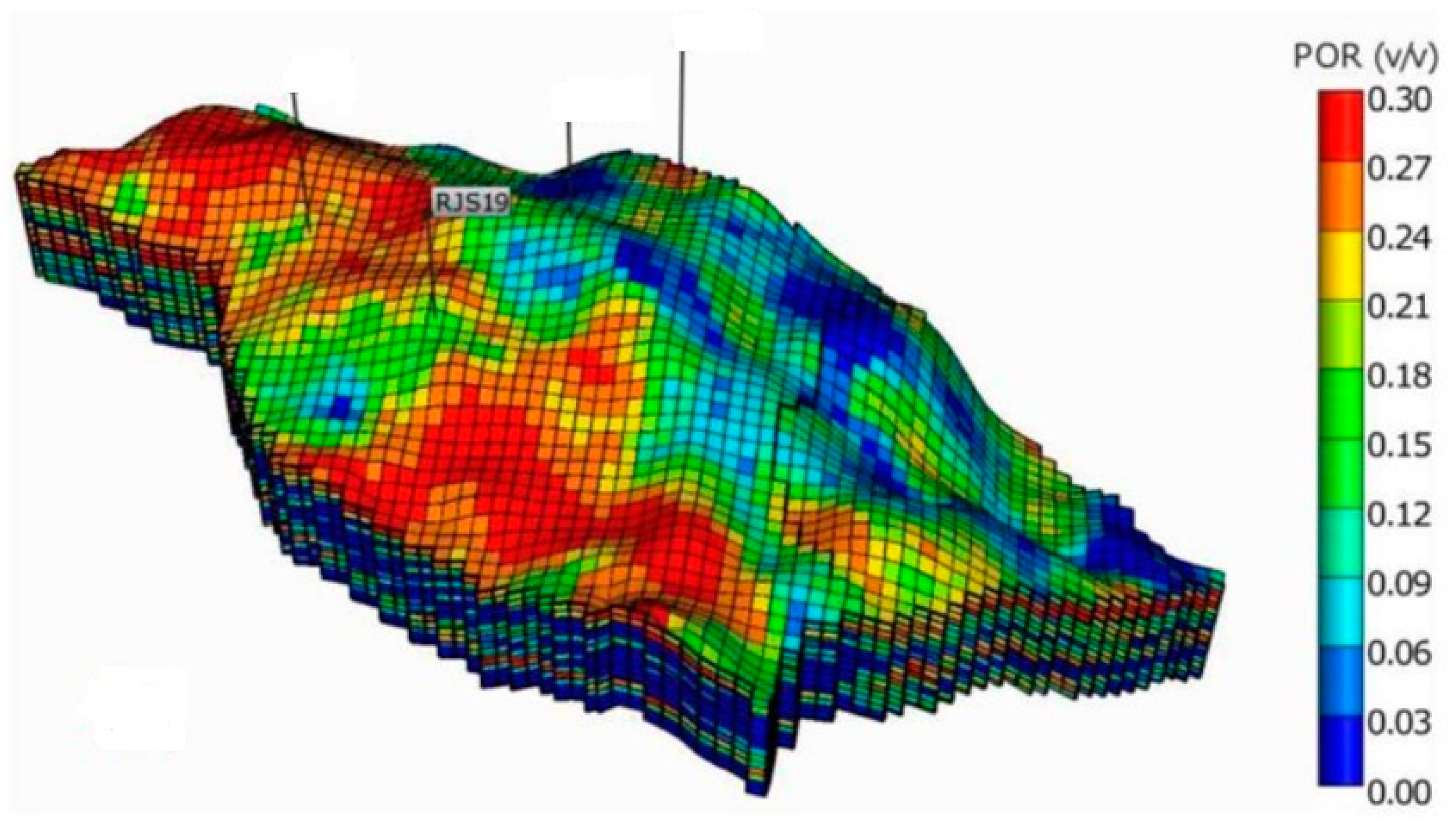
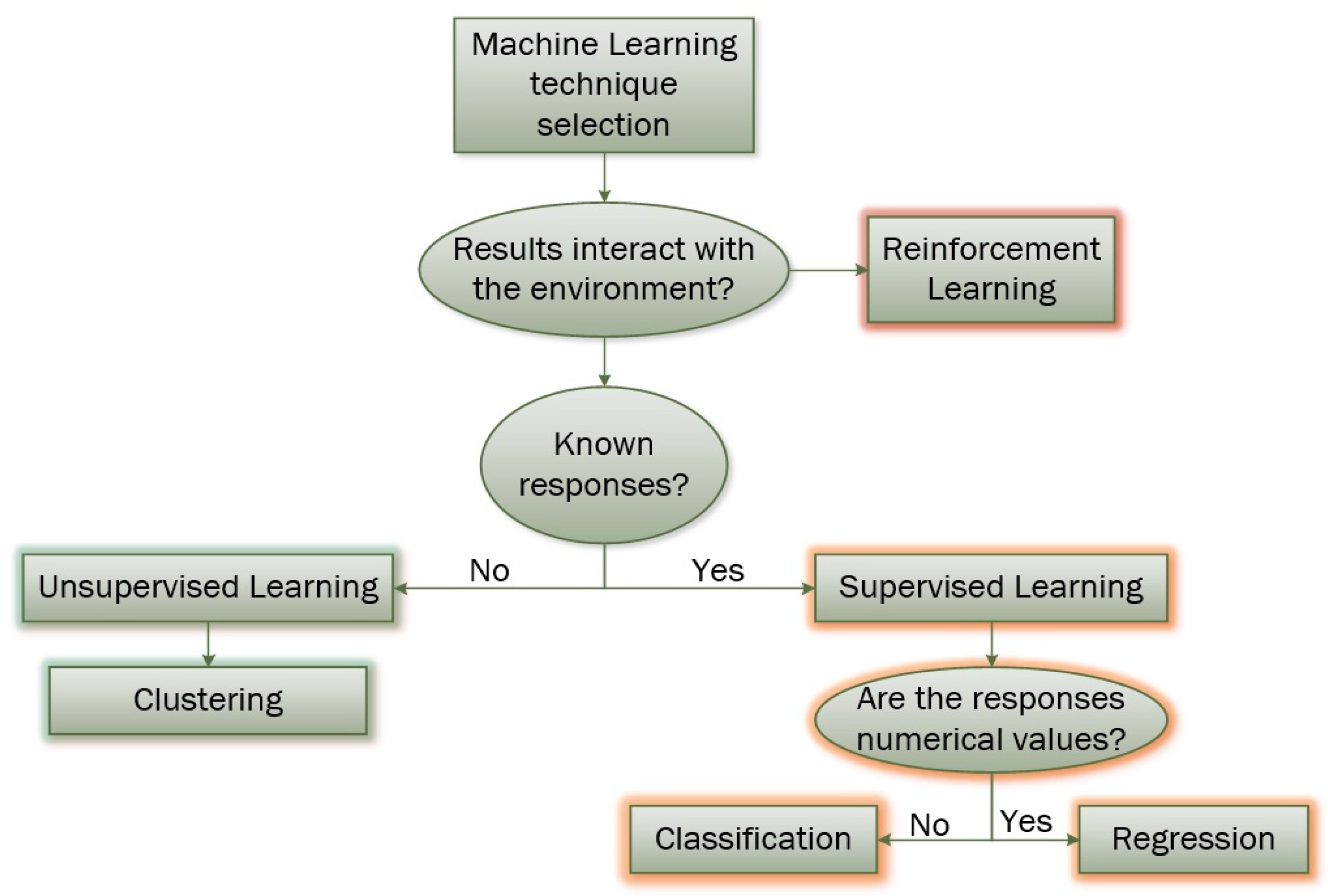
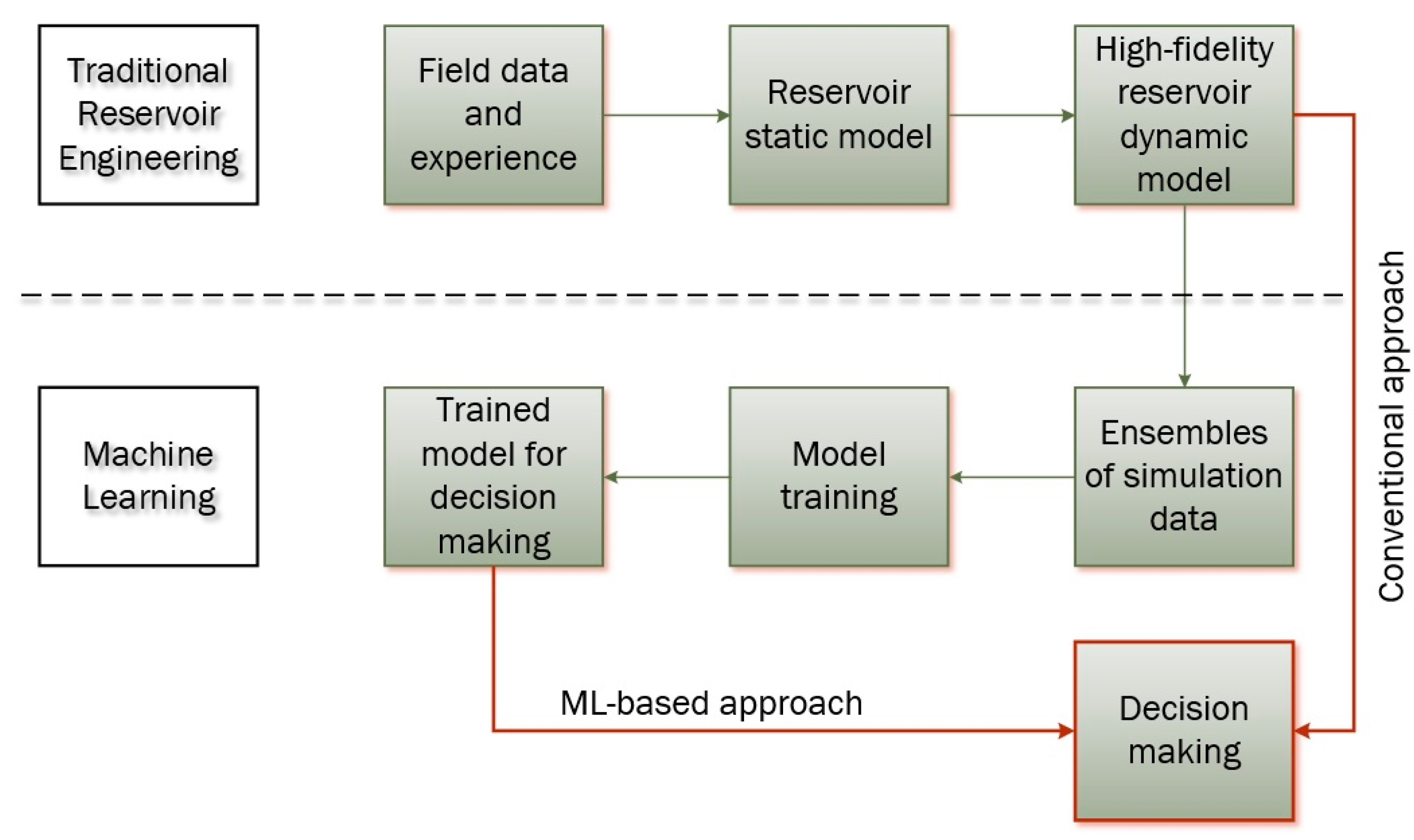
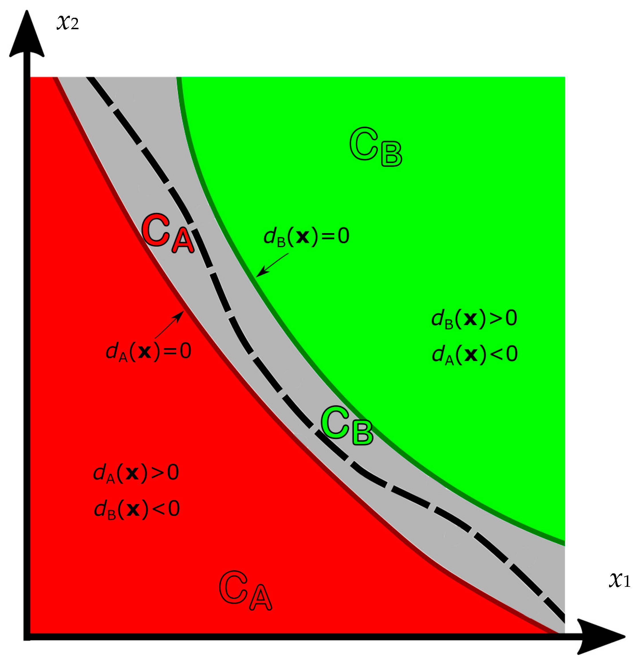
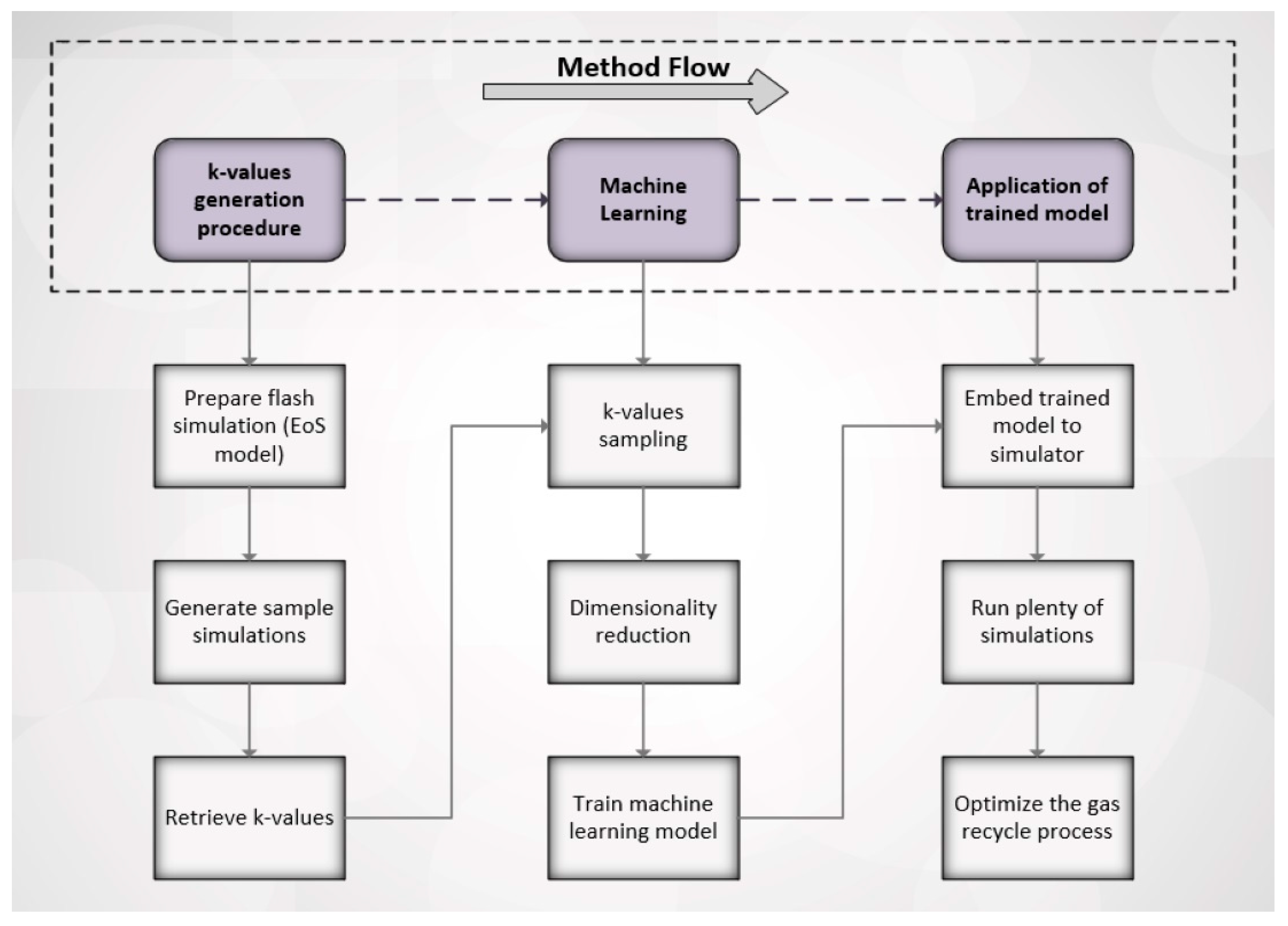
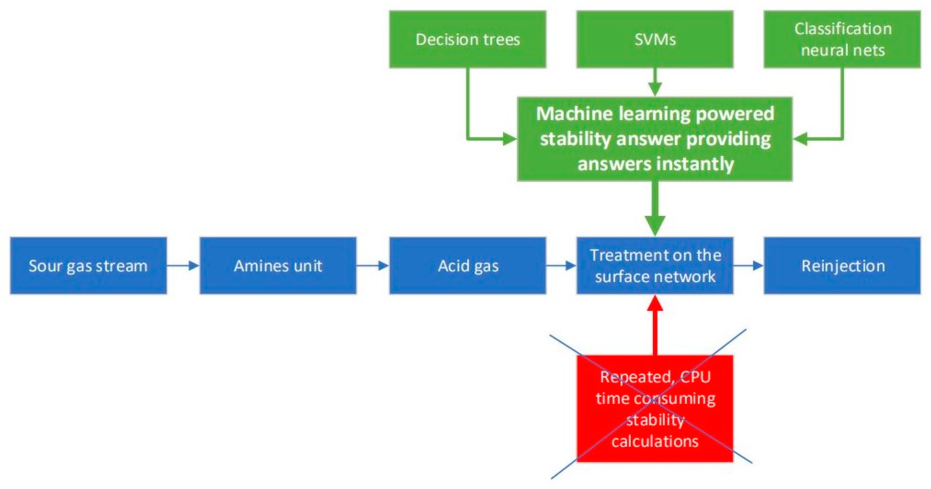
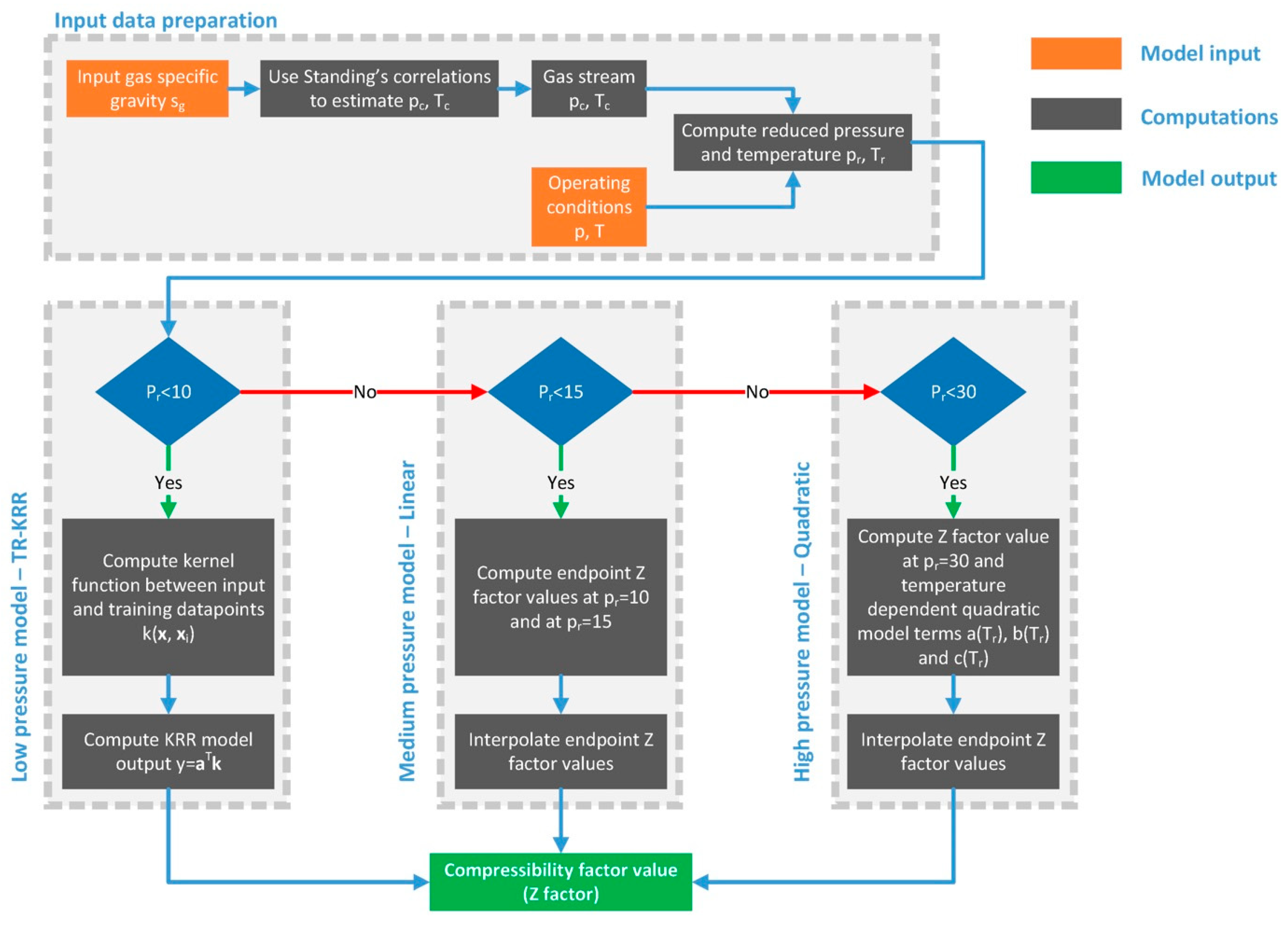
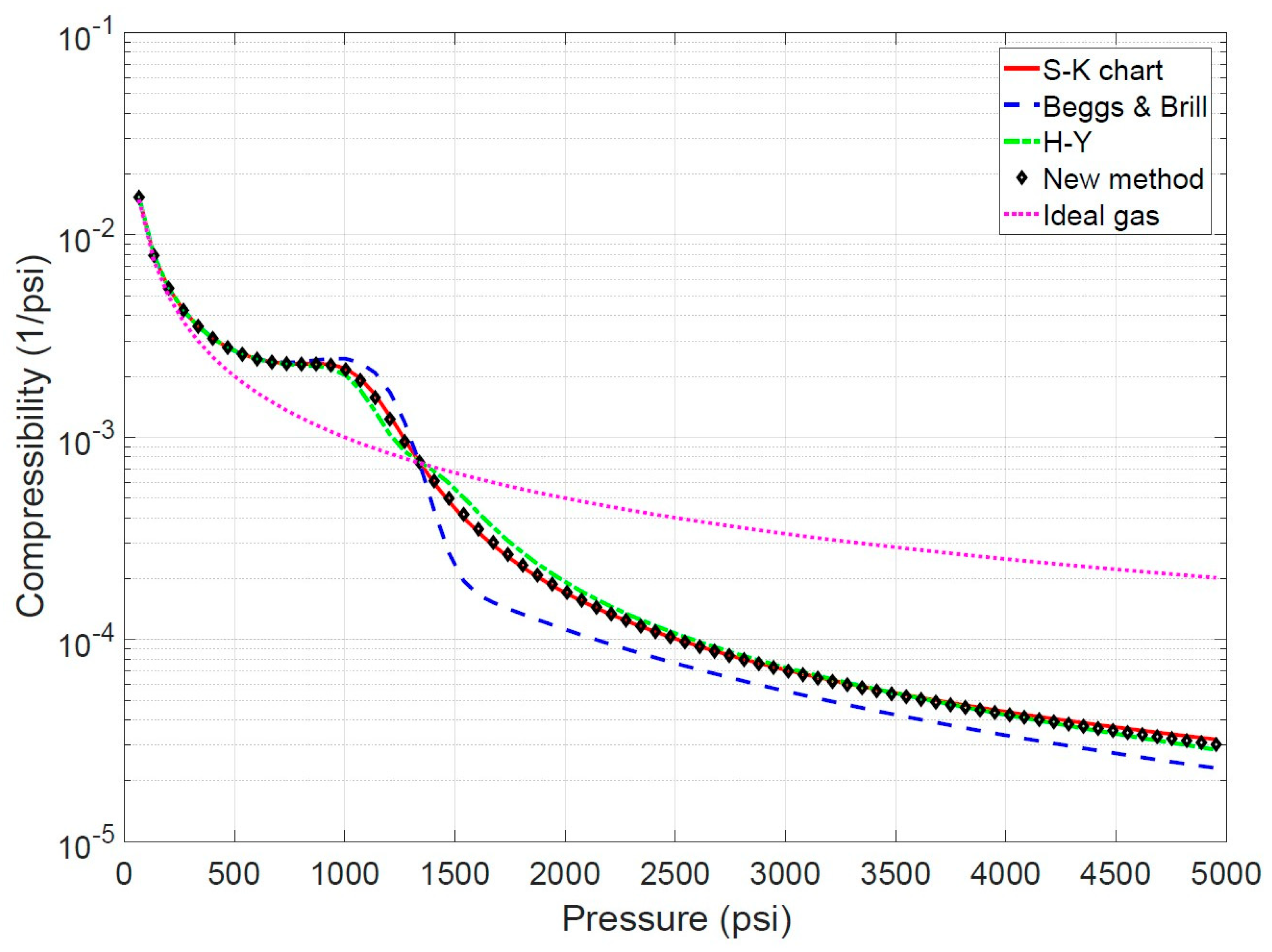
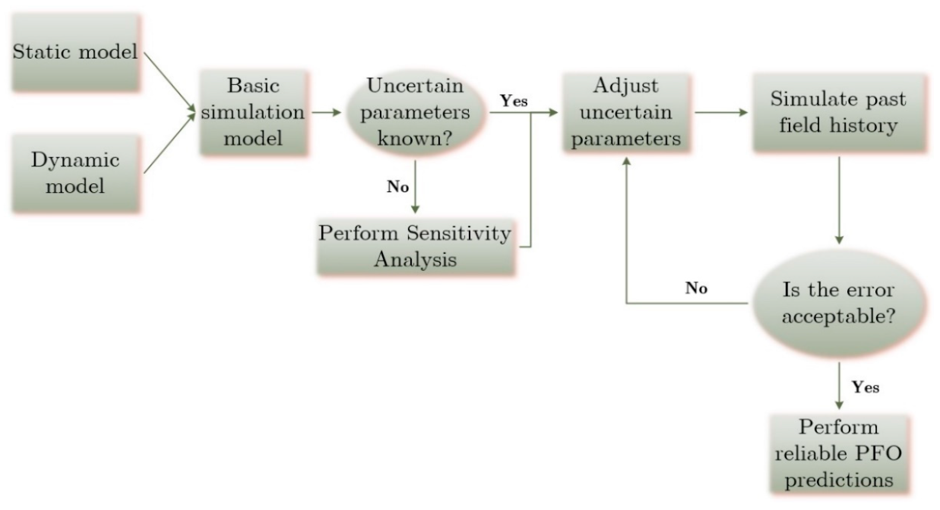
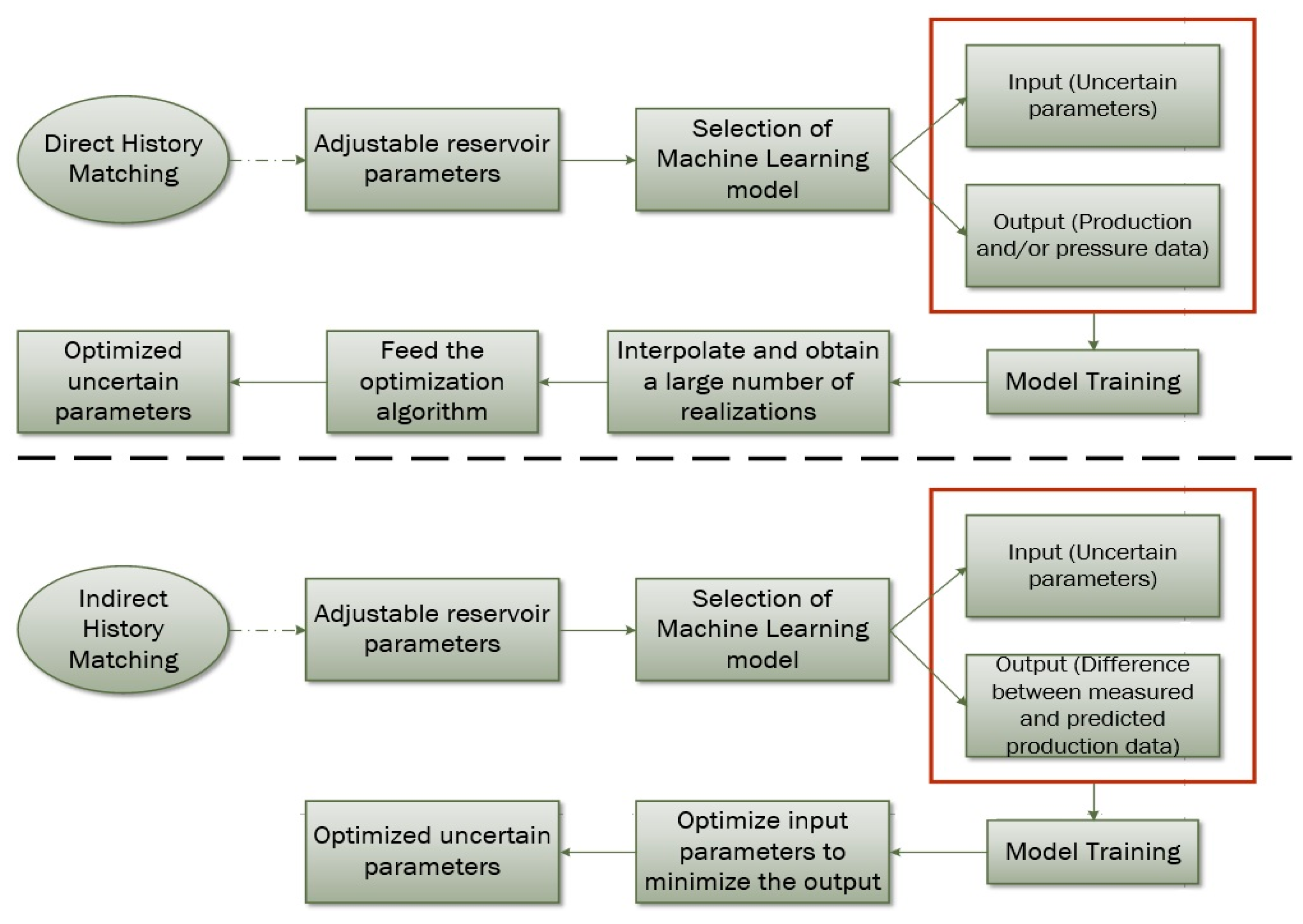
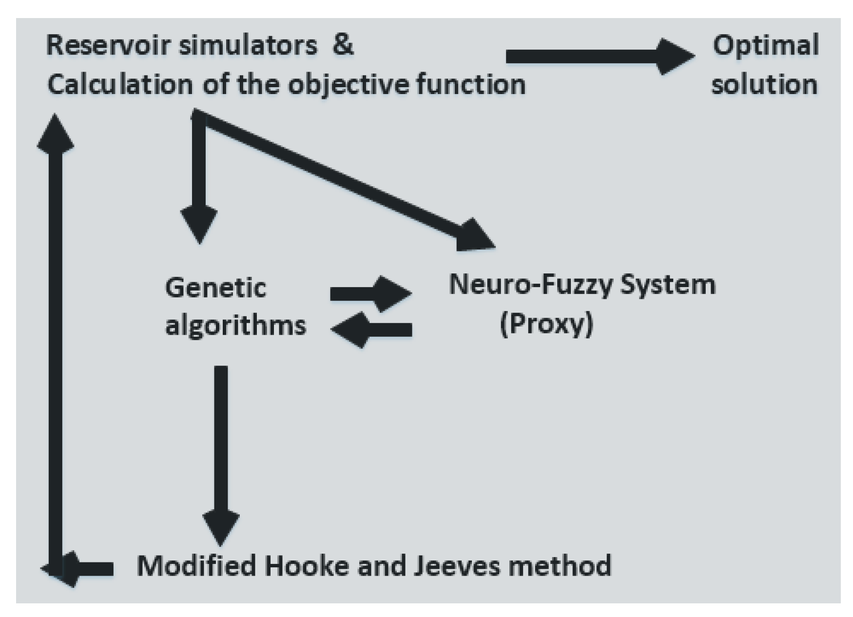
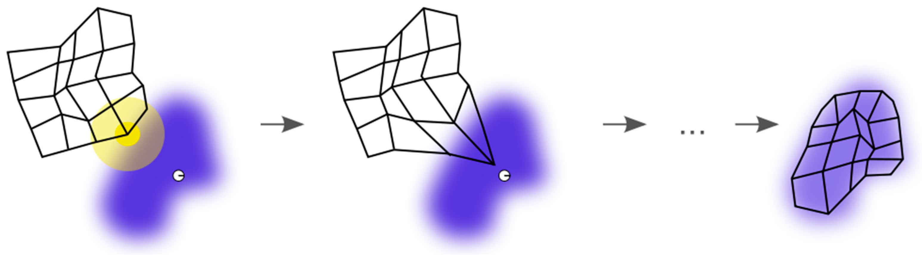
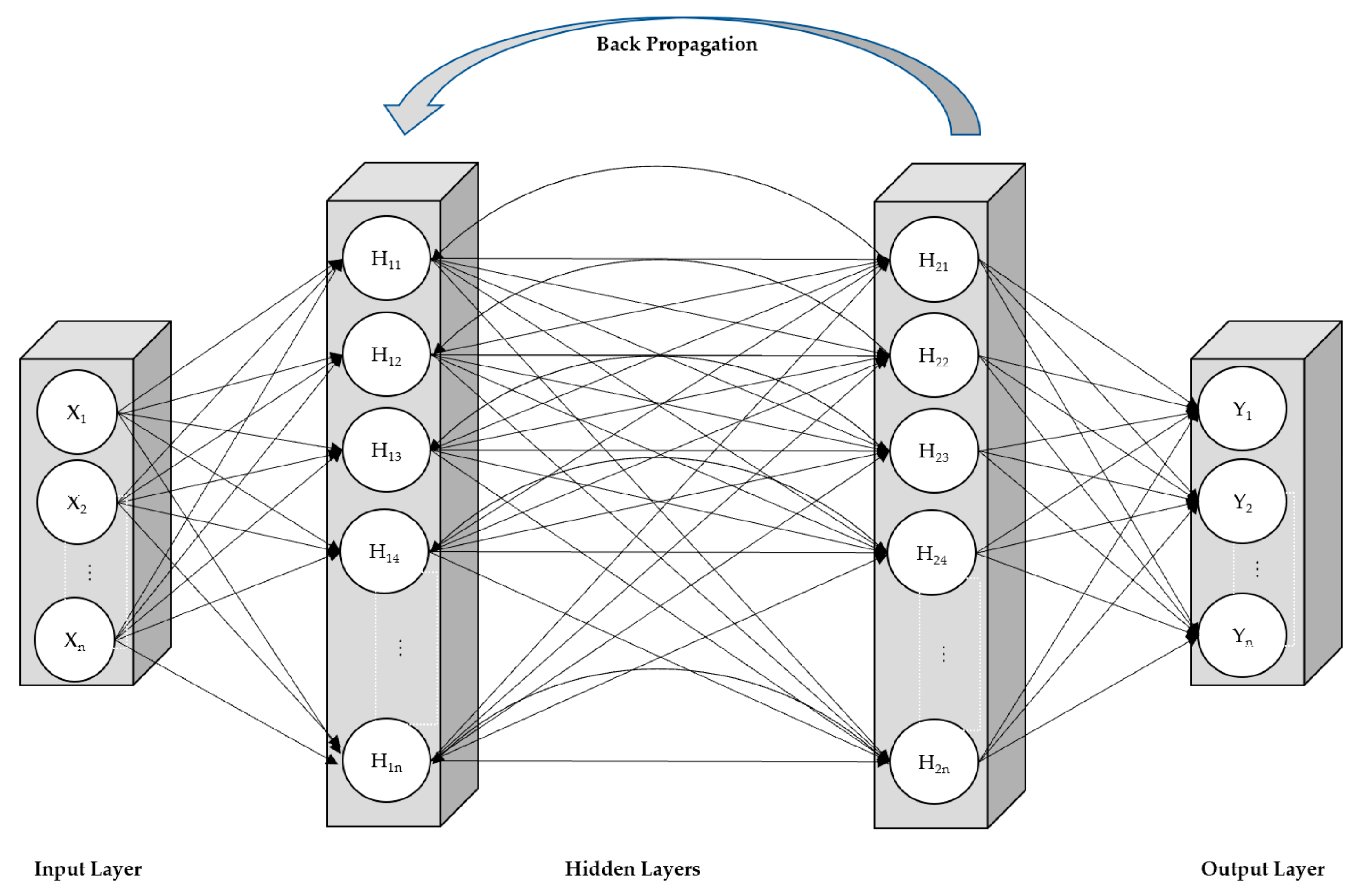
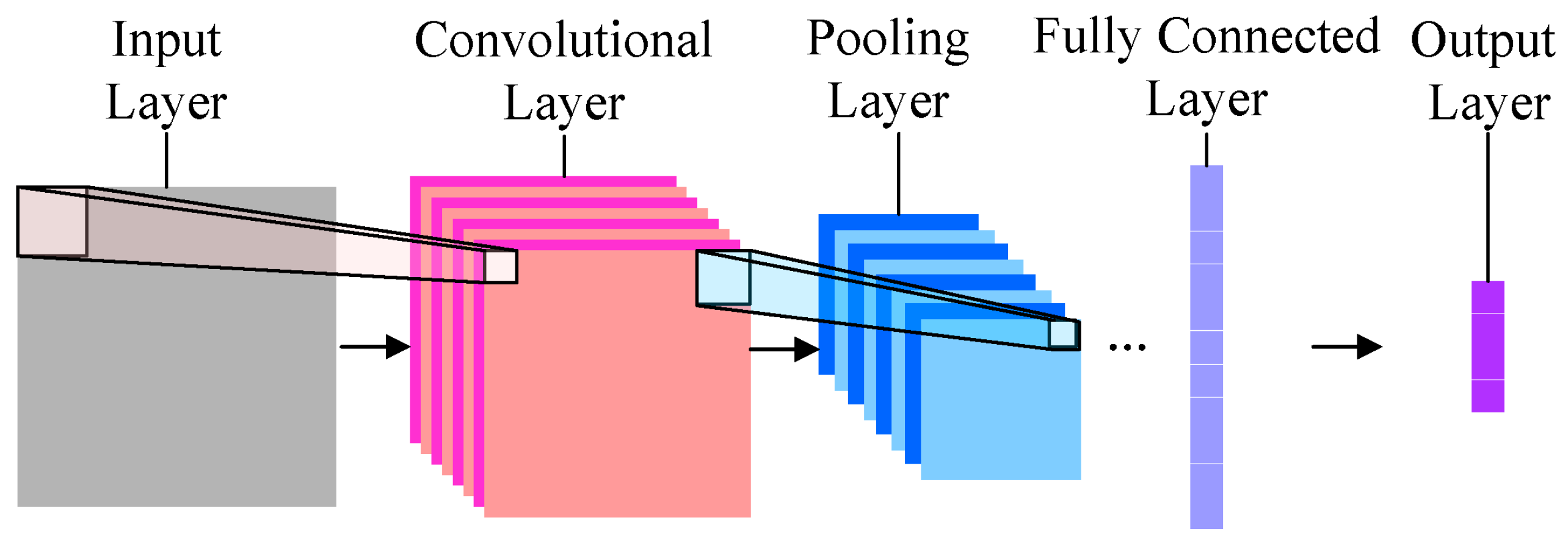
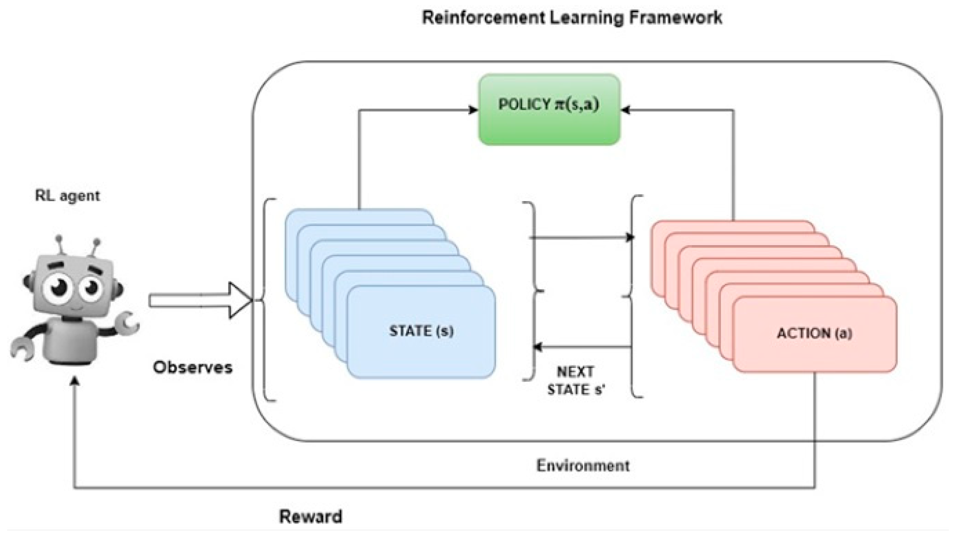
Table 1.
Individual simulation runs: applications summary.
| ML Application | ML Training Scheme | Main Objective | ML Method | Reviewed Studies (Reference List Number) |
|---|---|---|---|---|
| Surrogate Reservoir Models | Supervised | Hydraulic fracture | ANNs coupled with GA | [41] |
| Reservoir uncertainty analysis | [42,43,44,45,46] | |||
| Prediction of dynamic reservoir properties | ANNs | [1] | ||
| Water flooding reservoir simulation | [47] | |||
| CO2 storage—prediction of dynamic reservoir properties | [14,48,49,52] | |||
| Shale gas reservoir simulation | [50] | |||
| BHP predictions | RBFNN | [51] | ||
| Stability and phase split problems using k-values | Supervised | Phase stability | SVMs and ANNs | [39,53,55,57,58] |
| Phase stability/split | [10,54,56,59,65] | |||
| Phase split | [22] | |||
| Phase split | Deep learning ANNs | [60,64] | ||
| Phase stability/split | [61,62,63] | |||
| Black oil PVT properties | Supervised | Z-factor prediction | ANNs | [67,70,71,72,73,74] |
| SVMs and LSSVM with optimization methods | [75,76,78,83] | |||
| Kernel Ridge Regression | [80] | |||
| Saturation pressure | ANNs | [77,85,92,95,96] | ||
| SVMs | [90,91] | |||
| ANFIS | [93] | |||
| ANNs coupled with optimization methods | [97,98] | |||
| SVMs and LSSVM with optimization methods | [99,100,102] | |||
| SVMs and DTs | [101] |
Table 2.
History matching: applications summary.
| ML Application | ML Training Scheme | ML and Optimization Methods (If Any) | Reviewed Studies (Reference List Number) |
|---|---|---|---|
| Indirect history matching | Supervised | ANNs with stochastic optimization | [106,107] |
| ANNs with dimensionality reduction methods | [108] | ||
| Ensembles of ANNs | [109] | ||
| RBFNNs, Generalized Regression ANNs, FSSC and ANFIS stochastic optimization | [110,111,112] | ||
| Direct history matching | Supervised | ANNs | [114,115,116,117,118,119,120,126] |
| Bayesian ML models | [121,122,124,125] | ||
| MARS, DTs, single-pass GRNNs | [127] | ||
| Unsupervised | Self-Organizing Map (SOM) | [131] | |
| Supervised | SVR with dimensionality reduction and optimization | [135] | |
| RNN | [142,143] | ||
| CNN | [148,158] | ||
| Unsupervised | GAN | [149,159] | |
| Piecewise Reconstruction from a Dictionary (PRaD) with pluri-PCA | [151] | ||
| Convolutional AutoEncoders | [152,157] | ||
| Reinforcement learning | Reinforcement learning models | [103,162] |
Disclaimer/Publisher’s Note: The statements, opinions and data contained in all publications are solely those of the individual author(s) and contributor(s) and not of MDPI and/or the editor(s). MDPI and/or the editor(s) disclaim responsibility for any injury to people or property resulting from any ideas, methods, instructions or products referred to in the content. |
© 2023 by the authors. Licensee MDPI, Basel, Switzerland. This article is an open access article distributed under the terms and conditions of the Creative Commons Attribution (CC BY) license (https://creativecommons.org/licenses/by/4.0/).
Share and Cite
MDPI and ACS Style
Samnioti, A.; Gaganis, V. Applications of Machine Learning in Subsurface Reservoir Simulation—A Review—Part I. Energies 2023, 16, 6079. https://0-doi-org.brum.beds.ac.uk/10.3390/en16166079
AMA Style
Samnioti A, Gaganis V. Applications of Machine Learning in Subsurface Reservoir Simulation—A Review—Part I. Energies. 2023; 16(16):6079. https://0-doi-org.brum.beds.ac.uk/10.3390/en16166079
Chicago/Turabian StyleSamnioti, Anna, and Vassilis Gaganis. 2023. "Applications of Machine Learning in Subsurface Reservoir Simulation—A Review—Part I" Energies 16, no. 16: 6079. https://0-doi-org.brum.beds.ac.uk/10.3390/en16166079
Note that from the first issue of 2016, this journal uses article numbers instead of page numbers. See further details here.