Article

Proxy Model Development for the Optimization of Water Alternating CO2 Gas for Enhanced Oil Recovery

by
D Aqnan Marusaha Matthew
1,
Ashkan Jahanbani Ghahfarokhi
1,*,
Cuthbert Shang Wui Ng
1 and
Menad Nait Amar
2
1
Department of Geoscience and Petroleum, Norwegian University of Science and Technology, 7031 Trondheim, Norway
2
Departement Etudes Thermodynamiques, Division Laboratoires, Sonatrach, Boumerdes 35000, Algeria
*
Author to whom correspondence should be addressed.
Submission received: 7 February 2023 / Revised: 28 March 2023 / Accepted: 5 April 2023 / Published: 9 April 2023

Abstract

:
Optimization studies are an important task in reservoir engineering practices such as production optimization and EOR (Enhanced Oil Recovery) assessments. However, they are extensive studies with many simulations that require huge computational effort and resources. In terms of EOR, CO2 injection is one of the most common methods employed due to a high recovery potential and environmental benefits. To assess the feasibility of CO2-EOR projects, a reservoir design study must be conducted before optimization is performed. Some studies have demonstrated the advantages of employing proxy models to perform this task in terms of saving huge amounts of computer memory space and time. In this study, proxy models were developed to solve a multi-objective optimization problem using NSGA-II (Non-dominated Sorting Genetic Algorithm II) in two selected reservoir models. The study was performed for a CO2-WAG (Water Alternating Gas) application, where gas and water injection rates and half-cycle lengths were assessed to maximize the oil recovery and CO2 stored in the reservoir. One model represents a simple geological model (the Egg Model), while the other represents a complex model (the Gullfaks Model). In this study, the good performance of the proxy models generated accurate results that could be improved by increasing the amount of sampling and segmenting the behavior of the reservoir model (depending on the complexity of the reservoir model). The developed proxies have an average error of less than 2% (compared with simulation results) and are concluded to be robust based on the blind test results. It has also been found that to reach the maximum oil recovery using CO2-WAG, the maximum gas injection rate with the minimum water injection rate is required. However, this configuration may result in a reduction in the total CO2 stored in the reservoir.

1. Introduction

Global energy demand declined by 3.8% in the first quarter of 2020, where oil demand was hit strongly (by about 5%) due to the pandemic [1]. Albeit that the pandemic shifted the common behavior from work-from-office to work-from-home and caused a sharp reduction in non-essential activities, it is predicted that the oil demand will rebound to 2019 levels in 2023 [1]. This prediction is based on the recovery of the global economy, as the pandemic had a diverse impact across countries [2]. The growth needs to be balanced by supply, yet the global oil supply was adversely impacted due to project delays and demand uncertainty. The current active projects are barely able to fulfill the demand growth until 2026 [3]. At the same time, some companies have shifted focus and business models based on the demand from governments and activists to move towards net zero carbon emissions in 2050 [3].
The pandemic has also been one of the reasons for the renewable energy growth. By 2020, the growth in capacity of renewable energy generation, dominated by the increase in solar and wind energy capacities, increased by 10.3% compared to 2020 [4]. Efforts to reduce the dependency on fossil fuels have also emerged, but some measures were affected by the pandemic. The price of the carbon tax, pricing initiatives, allowance prices, and key meetings have been reduced and these initiatives have been delayed due to the uncertainty of the market [5]. Despite this situation, several countries such as Germany and China are planning to join the carbon tax plan (planned in 2021) [5]. This plan will create a paradigm shift in the operation plans for oil companies in these countries by adding extra constraints in tax calculation, i.e., emissions tax, given that the volatility of the oil price and demand will exist even after the pandemic.
Fulfilling the oil demand while reducing carbon footprint are considered two tasks that refute each other. Producing negative emission is challenging for the oil industry as a lot of parameters are involved in every stage of the reservoir exploitation. Nonetheless, near-zero emission is attainable in some conditions. The Johan Sverdrup field (operated by Equinor), for example, emits only 4% of the world’s average CO2 emissions per barrel of oil produced due to the power from shore [6]. Preplanning during exploration is important, but most existing fields were not preplanned as well as this field. Considering the decline in production in most existing fields, an alternative approach to reach the climate targets and meet the energy demands is CO2 Enhanced Oil Recovery (EOR). CO2-EOR is considered as one of the answers to satisfy the demand in carbon capture, utilization and storage (CCUS), while retaining the profit [7].
Assessing the feasibility of EOR projects requires several evaluations before field-scale application. Aside from the common steps, viz. technical and economical screening, reservoir design is needed for CO2-EOR [8]. Several considerations, for instance, the injection design, rate, cycle, composition, and existing field constraints, are accounted for in this phase. In the context of CO2-EOR injection design, water-alternating-gas (WAG) has been proven as one of the best designs [9]. CO2-WAG increases the microscopic displacement efficiency and yields a better mobility control to contact the unswept zones compared to continuous flooding. To design the parameters of the process, optimization needs to be performed. Optimization is a computationally expensive study, as numerous runs are required to solve the problem. Running optimization using existing reservoir simulators demands extensive amounts of time and memory space to solve the problem.
Building proxy models to solve the optimization problem is commonly performed for study assessment. A proxy model is a mathematically or statistically defined function that replicates the numerical simulation model outputs given selected input parameters. The ability of proxy models to learn complex reservoir model behavior has been proven in recent studies using both synthetic and field models [10]. A proxy model learns from the given training and validation data generated from the response surface or simulation model output. A proxy model is an engineering tool that also honors the physics of the problem at hand. This powerful tool is constructed based on managing, clustering, and filtering data into information, later learned as knowledge.
The primary objective of this work (which is mainly based on the results obtained in [11]) is to find a strategy that allows a significant reduction in runtime and storage space associated with the commercial simulators without sacrificing accuracy. This study is performed using CO2-WAG as one of the most common Enhanced Oil Recovery (EOR) methods. A proxy model is built as a reservoir model substitute, and the total oil produced and CO2 stored will be maximized as the objective function of the optimization problem. This study will be performed on two geological models, where one acts as a simple model, while the other represents the complexity that is expected in a real field model. Several points that are studied in this research are:
  • Development of a proxy model for simple and complex reservoir models that involves sampling using experiments, proxy buildings, and proxy robustness assessments.
  • Analysis of the problem and complexity encountered when building a proxy of a complex reservoir model, in comparison with the results of a simple reservoir model proxy development.
  • Solving the optimization problem with the generated proxy, both for the simple and complex reservoir models, using an optimization algorithm.
The paper is divided into several sections. Section 1 introduces the background and the objective. Section 2 summarizes the basic theory and workflow of the study. Section 3 describes the materials and method to solve the optimization problem. Section 4 focuses on the details of how the proxy model is built to solve the optimization problem. The Section 5 describes the results of the two proxy models. Finally, the discussion and conclusions are presented in the last two sections.

2. Basic Theory

2.1. Previous Study on Proxy Modeling

The study of proxy models was initiated in the 2000s in the field of petroleum/reservoir engineering, mostly to solve computationally expensive problems. Zubarev [10] reviewed the growth of proxy model studies from 1998 to 2008. They found that all proxy modeling techniques showed dependence on the complexity of the reservoir model, solution space dimensions, and the dataset quality.
Gholami [12] applied a proxy model or a surrogate reservoir model (SRM) in their study of a complex problem, where a smaller elemental volume was studied. The study was applied to CO2-WAG to mimic the grid behaviors (pressure and saturation) and well-based behaviors (production rates of oil, gas, and water). Based on the study results, the constructed proxy model learned the preferred pressure, saturation, and rate behavior, in which one year was used as the timestep interval for reporting frequency.
Amini [13] performed a detailed study for a grid-based proxy model following Gholami’s results. The cascading effect (in which error is carried over and accumulates by iteration) and a comparison between fine-grid and coarse-grid reservoir models were analyzed in a CO2 sequestration study. The study showed that the coarser model required fewer runs for training purposes than the fine grid model. In alignment with that, the cascading procedure illustrated significant errors when observed in the last time step.
In one of the recent studies performed by Chaki et al. [14], they developed a proxy model to perform history matching using the Brugge field model as the reservoir model to be learned. They applied two methods, a deep neural network (DNN) and a recurrent neural network (RNN), to build a proxy that learns the behavior of the reservoir model (oil and water production rate and cumulative production). The RNN demonstrated better performance than the DNN, yet the amount of time needed to construct it was 15 times higher than that for the DNN.
Nait Amar et al. [15,16] performed a CO2-WAG optimization study using proxy models. Two different machine learning (ML) techniques, namely an ANN [15] and a hybrid support vector [16], were implemented. These developed ML-based proxy models were able to learn the reservoir behavior (oil and water rate) and were then coupled with nature-inspired algorithms for the CO2-WAG optimization study. Besides that, a study also demonstrated how an ANN could be employed to build a proxy model for waterflooding optimization in a fractured reservoir model [17]. Thereafter, this study was extended to improve the methodology as discussed in [18].

2.2. Possibilities for Proxy Modeling Improvement

Although many studies related to proxy modeling have been performed, there are still research gaps to be filled. Most studies showed that a proxy model could be a powerful tool for various tasks, including predictive models related to CO2 and H2 property estimations [19,20] and substitutes for reservoir models as detailed in the previous section. In the domain of reservoir and production engineering, proxy models can provide an alternative to overcome the current computational limitations in reservoir modeling (tremendous run time and memory consumption). In this aspect, most studies have worked with only one geological model and there are few studies focusing on the feasibility of this idea begin applied in different geological models (considering geological uncertainty) [21,22]. Some studies have also mentioned that the proxy would reflect the complexity of the reservoir model, yet quantitative results are to be found [14]. Therefore, an investigation was performed to check whether a proxy model is a feasible substitute for the reservoir models studied in this paper. It is worth noting that the proxy models are generally case specific.

2.3. Workflow

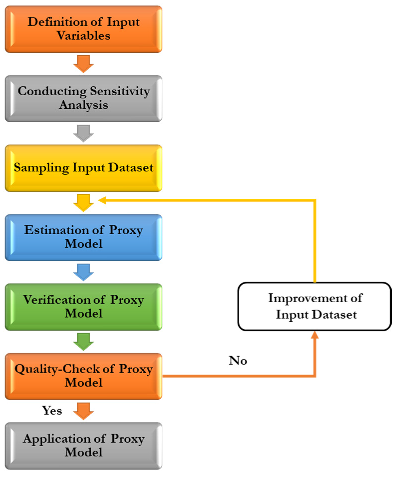
There are generally four big steps that can be used as a guideline for proxy modeling.
1
Determining the study objective:
A proxy model only learns from the given sets of data and information, and this creates a limitation for the model, making it case specific. Different proxies need to be built for different study objectives, leading to sampling, proxy input–output combinations, study limitations, and the requirement of algorithms to solve the problem.
2
Data sampling:
After determining the study objectives, proxy scale, and input data for the proxy, data sampling can be performed. Data sampling is usually performed by running the reservoir model. The results to be learned are then sampled for the proxy learning dataset. Data sampling can be performed using available statistical sampling.
3
Data management:
After obtaining the sampling plan, reservoir model runs will be performed. Many data points can be obtained, yet not all of them will be used for proxy model training.
4
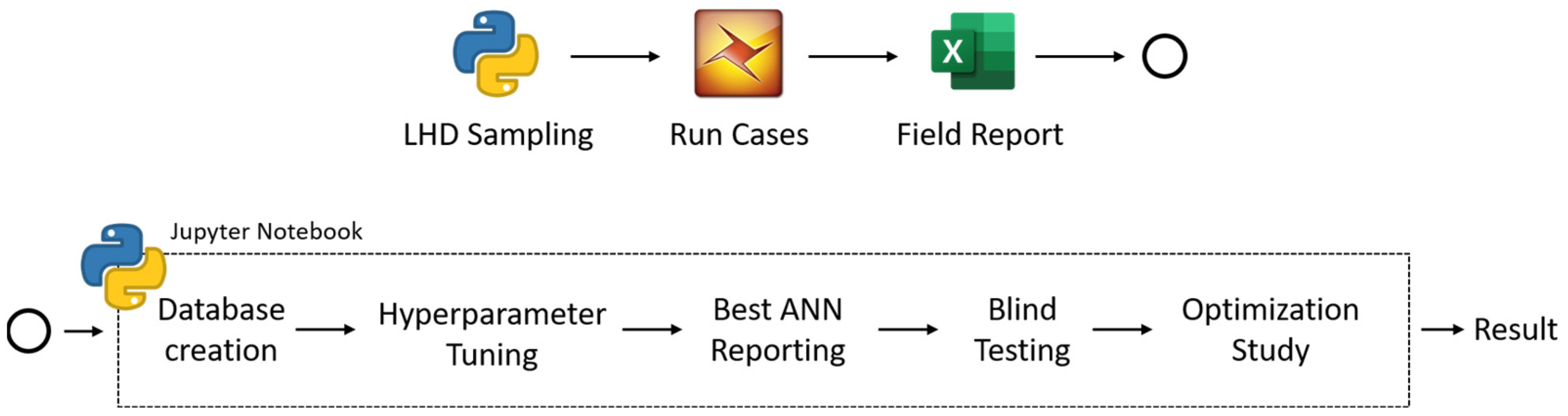
Designing and building the proxy model:
Using available machine learning or deep learning models, a proxy model can be built. The proxy model will approximate the numerical reservoir model. It should mimic the nonlinearity in responses of the numerical model. The complexity of the proxy model itself reflects the complexity of the reservoir model. Studies on proxy modeling have used approximately the same workflow shown in Figure 1.

2.4. Artificial Neural Network (ANN)

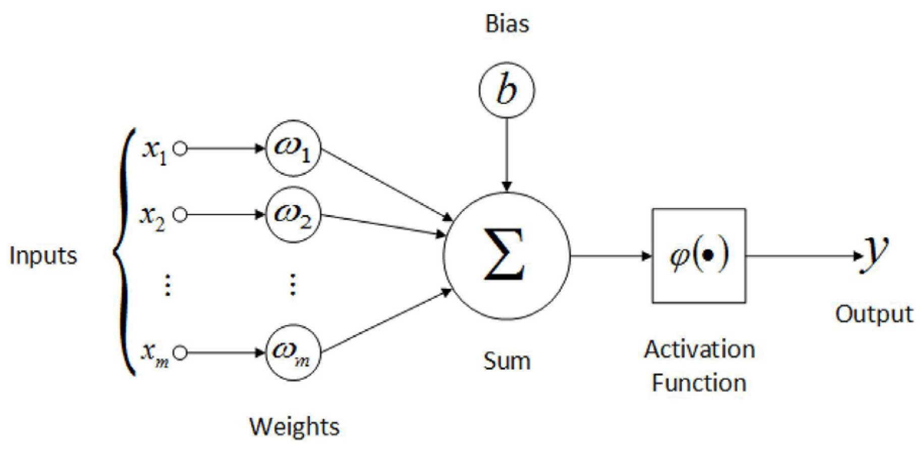
In this study, an ANN was used to build the proxy. An ANN is a computational model inspired by the biological behavior of the human neurological system. An ANN consists of inputs, weights, bias, and an activation function. The structure, formed of several layers, each containing several nodes before reaching the output, is called the topology (Figure 2). The activation function gives ANNs the ability to model the nonlinearity of a reservoir model. An ANN learns from forward and backpropagation, where the weights will be updated during each process to minimize the error. During forward propagation, the network moves from the input layer to the output layer, passing through each node and being transformed by the activation function, and eventually the results will be output. This will be noted as the neural network prediction.
The differences between the predicted and the actual output dataset are then calculated using a loss function, such as mean squared error (MSE), root mean square error (RMSE), absolute error (AE), and any other loss function. Backpropagation will then be performed to minimize the loss function. The loss will be sent back to the input layer as a fraction of the total signal of the loss. These two processes will be performed until the error satisfies the limit set or the number of iterations (epoch multiplied by batch size).
A hyperparameter is a parameter that controls the learning process. The activation function, number of hidden layers, and number of nodes are considered as hyperparameters in an ANN. Other than these, other hyperparameters such as learning rate, the optimizer, batch size, dropout, and number of epochs, are also considered. The learning rate is the step size for each iteration and the optimizer is the optimization function to minimize the loss function. The dropout is the probability that nodes are randomly disconnected during training and the batch size is the number of data points that pass through the neural network in every step. The epoch number is the number of cycles the training dataset goes through.

2.5. NSGA-II (Non-Dominated Sorting Genetic Algorithm II)

NSGA-II, an optimization algorithm to solve the multi-objective optimization problem, works based on genetic algorithms. A genetic algorithm is inspired from natural evolution theory. The algorithm reflects the natural selection process, where the fittest individuals are selected to reproduce the new offspring of the next generation. NSGA-II can be categorized as an evolutionary algorithm. This algorithm type was developed due to issues found in classical and gradient-based techniques, including the performance, which depends on the initial guess, and sub-optimal convergence issues. This algorithm uses a genetic algorithm as its fundamental knowledge. Three features of this algorithm are:
1
Elitist principle;
2
Explicit diversity preserving mechanism;
3
Emphasis on the non-dominated solutions.
The PyMoo [23] built-in is used to implement NGSA-II in this study. For an illustration of the NGSA-II procedure, please refer to the work in [24].

3. Materials and Methods

3.1. Reservoir Model

In this study, proxy models will be built to represent two reservoir models. One of these models is the simple model taken from Jansen, J.D. et al. [25], while the other one is developed from the Gullfaks K1/K2 dataset. Both proxies will solve the multi-objective optimization problem in the study of CO2-WAG design using the same optimization algorithm. An overview of the complexity difference between the models is listed in Table 1.
ECLIPSE 300 and PETREL were used as the simulator for running the models. It is worth noting that an identical relative permeability relationship is applied in both models that are shown in Figure 3. Both reservoirs have the same rock characteristics (sandstone), so the sand preset is used. The compaction function used for both models is the Newman correlation for consolidated sandstone rock. Both models are initialized using the same conditions as described in the fluid model data. This was done to ensure the miscibility conditions are identical, as it will be applied under different geological conditions.
The dimension of the grid for the Egg Model (used to visualize the performance difference between simulators) is considered small. This model is too small compared to the complex model in terms of volume. For this reason, the grid dimension was altered by multiplying by 3.125 (from 8 × 8 × 4 m to 25 × 25 × 12.5 m). This increases the volume to 30.5 times the original volume. The initial oil amount is then 16.5 million sm3 after initializing the fluid model.

3.2. Fluid Model

Both models are applied using the same fluid model, taken from Negahban, S. et al. [26]. The fluid model, categorized as light oil from its density, has a low viscosity (based on EOS tuning results) and fulfills the screening criteria of CO2-EOR by Al-Adasani [27] modeled with the Peng–Robinson equation. Constant composition expansion (CCE), differential liberation expansion (DL), multi-stage separator, slim tube, swelling, and multi-contact test data are available. These PVT test data are sufficient for fluid modeling in the CO2-EOR study. EOS PR78 was used in this study.
Due to the lack of molecular weight data on the matched pseudo-components, EOS tuning was performed on the available data. The primary process for EOS tuning here is splitting C20+ and regressing on conventional PVT test data (CCE, DL, multi-stage separator test). After that, lumping was performed into seven components. Regression was then performed based on the available advanced PVT tests (slim tube and swelling test). The matched PVT results are shown in Figure 4.

3.3. Depletion Scenario

Both models have about the same initial oil in place after the alteration (16.5 million sm3 for the Egg model and 17.2 million sm3 for the Gullfaks model). Both will be depleted for eight years, supported with water injection to keep the reservoirs undersaturated. Equal injection rates and production rate limits were applied to both models. All wells are active (producing and injecting), starting in 2013 and continuing to operate until 2021. Table 2 shows the depletion study details and results obtained from each model.
Test runs were also performed to test the performance of both reservoirs. A waterflooding study was performed to see the field performance compared to CO2-WAG. Figure 5 shows the results for both reservoirs. A higher recovery is seen when CO2-WAG is applied (3 months half-cycle, 6000 sm3/day field water injection rate, and 0.9 Msm3/day field gas injection rate) compared to waterflooding (3000 sm3/day field injection rate).

3.4. Optimization Study

Objective Function

The two results that will be analyzed are the field total oil production (FOPT) and CO2 stored in the reservoir. Based on this, two objective functions need to be defined. The parameters that will be studied are the half-cycle length (HC), the field gas injection rate (qg), and the field water injection rate (qw), with several segmentations and ranges. These are formulated as follows:
m a x i m i z e F O P T = n = 1 122 F O P R H C , q g , q w n · 30 C O 2 S t o r e d = q g · t g , i n j e c t n = 1 122 F C O 2 P R H C , q g , q w n · 30 s u b j e c t t o H C = 3 , 6 , 9 , 12   m o n t h s 1   M s m 3 / d q g 2   M s m 3 / d 3000   s m 3 / d q w 9000   s m 3 / d

4. Proxy Development Workflow

In this section, the proxy development process is explained briefly and performed for both reservoir models.

4.1. Design of Experiments

The sampling was performed using LHS (Latin Hypercube Sampling) [28] in this study. This sampling can be considered as a leveled sampling. It was performed based on previous study results and successful work on sampling for the study of WAG, for example, by Nait Amar, M. et al. [16]. The two levels of sampling that were performed in this study are as follows.
  • Half-cycle length:
    Sampling was performed for 3, 6, 9, and 12 month half-cycle lengths. This means that the proxy will not predict the CO2-WAG behavior out of the half-cycle length correctly.
2.
Gas injection rate and water injection rate:
The gas injection and water injection rates are sampled for each possible half-cycle length equally, since the probability for half-cycle length is equal for each possible value. More samples can be added if the proxy cannot learn from the given number of samples. The distribution of this parameter probability is uniform. Parameters are not dominating the others. Hence, the usual LHS can be performed.

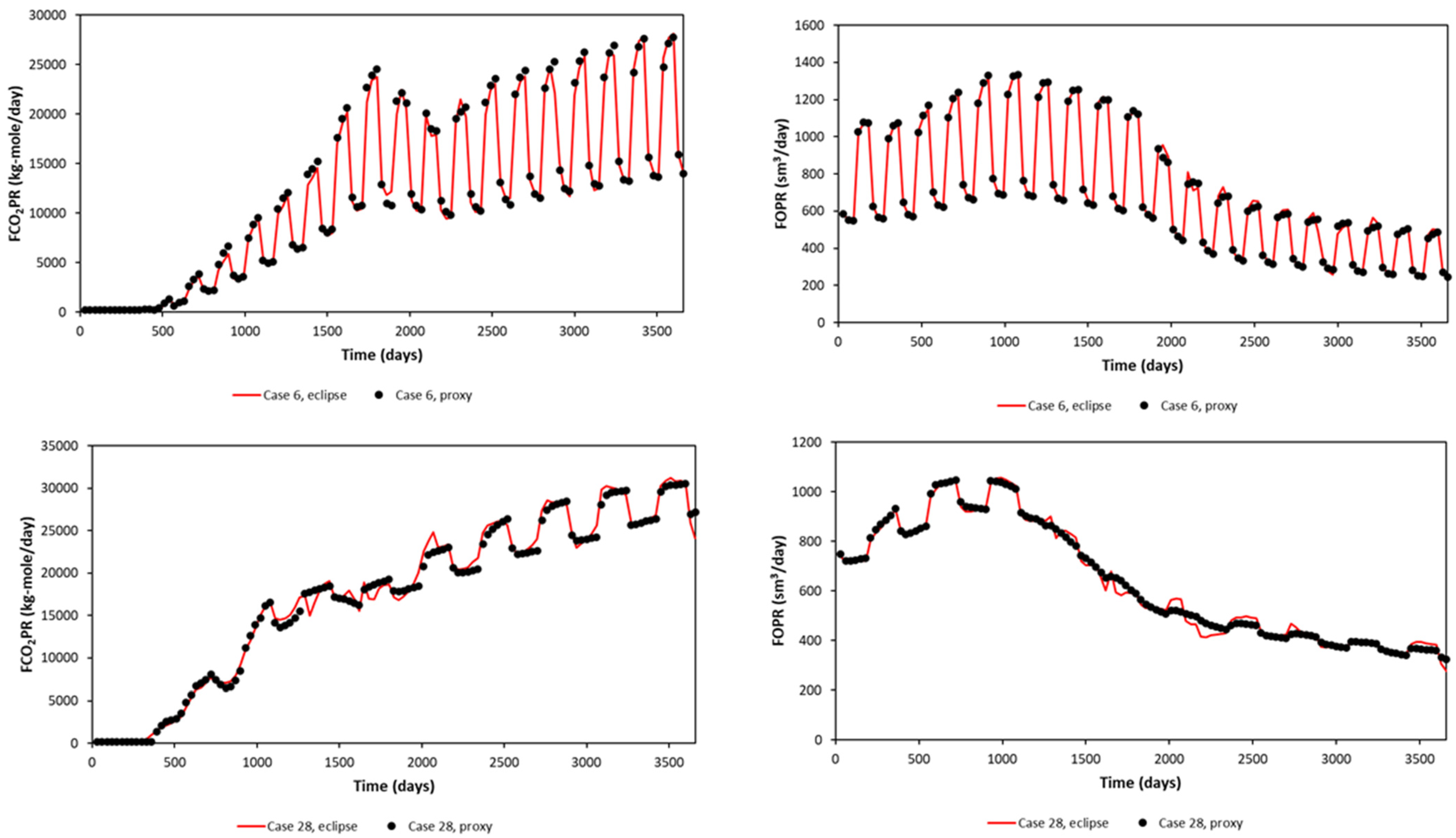
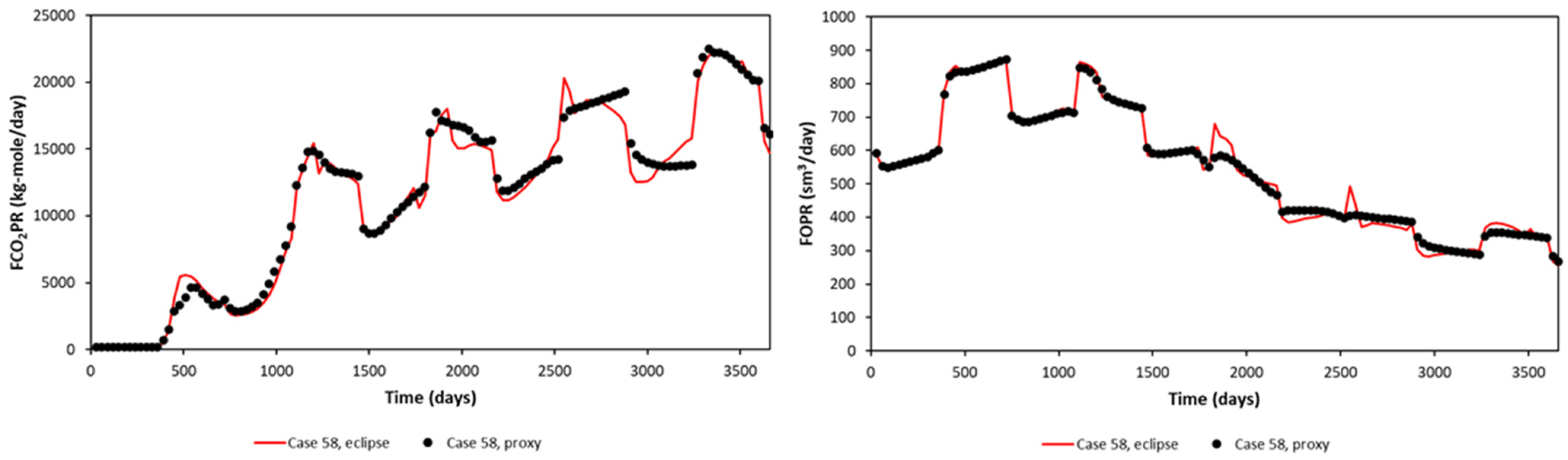
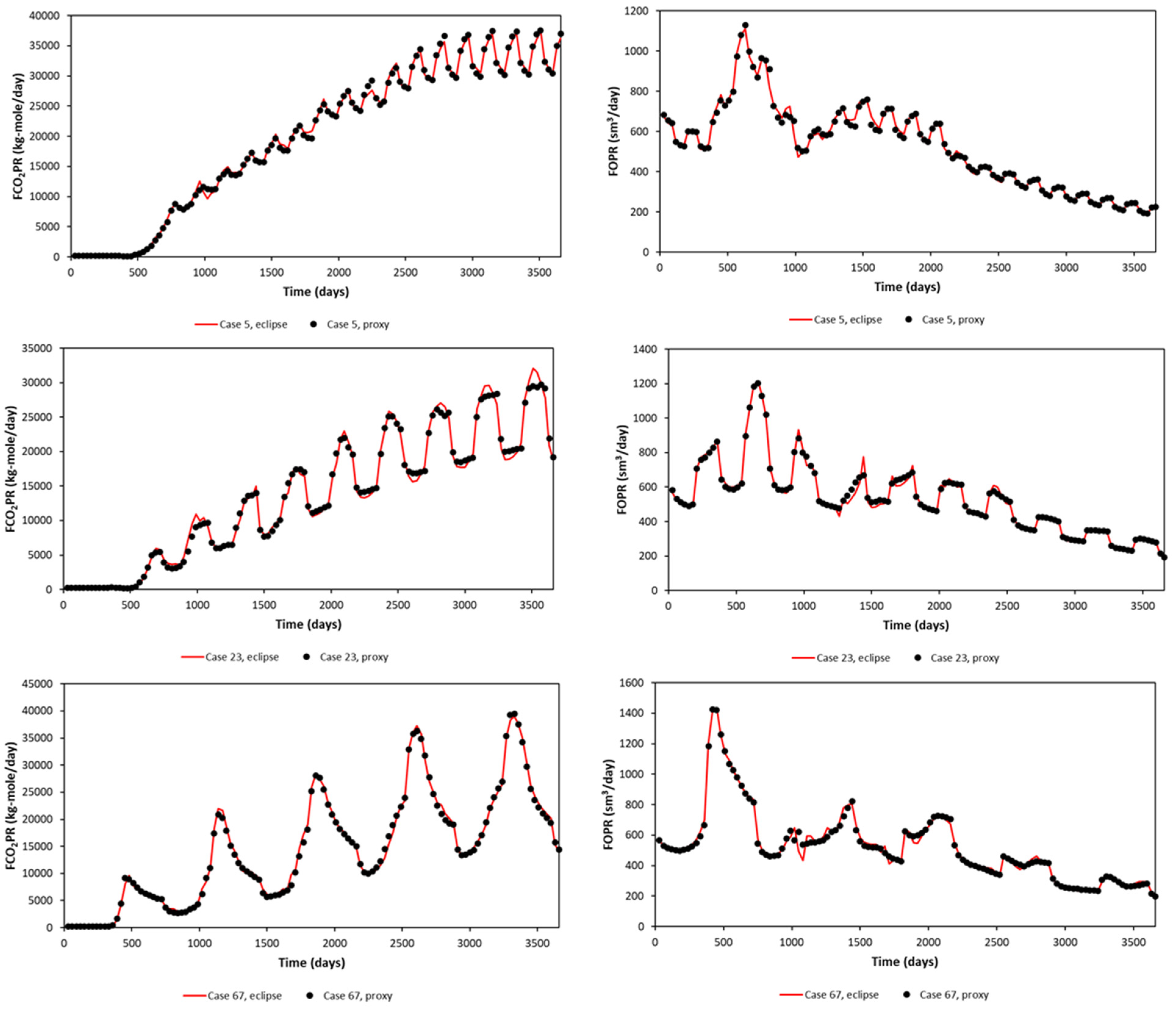
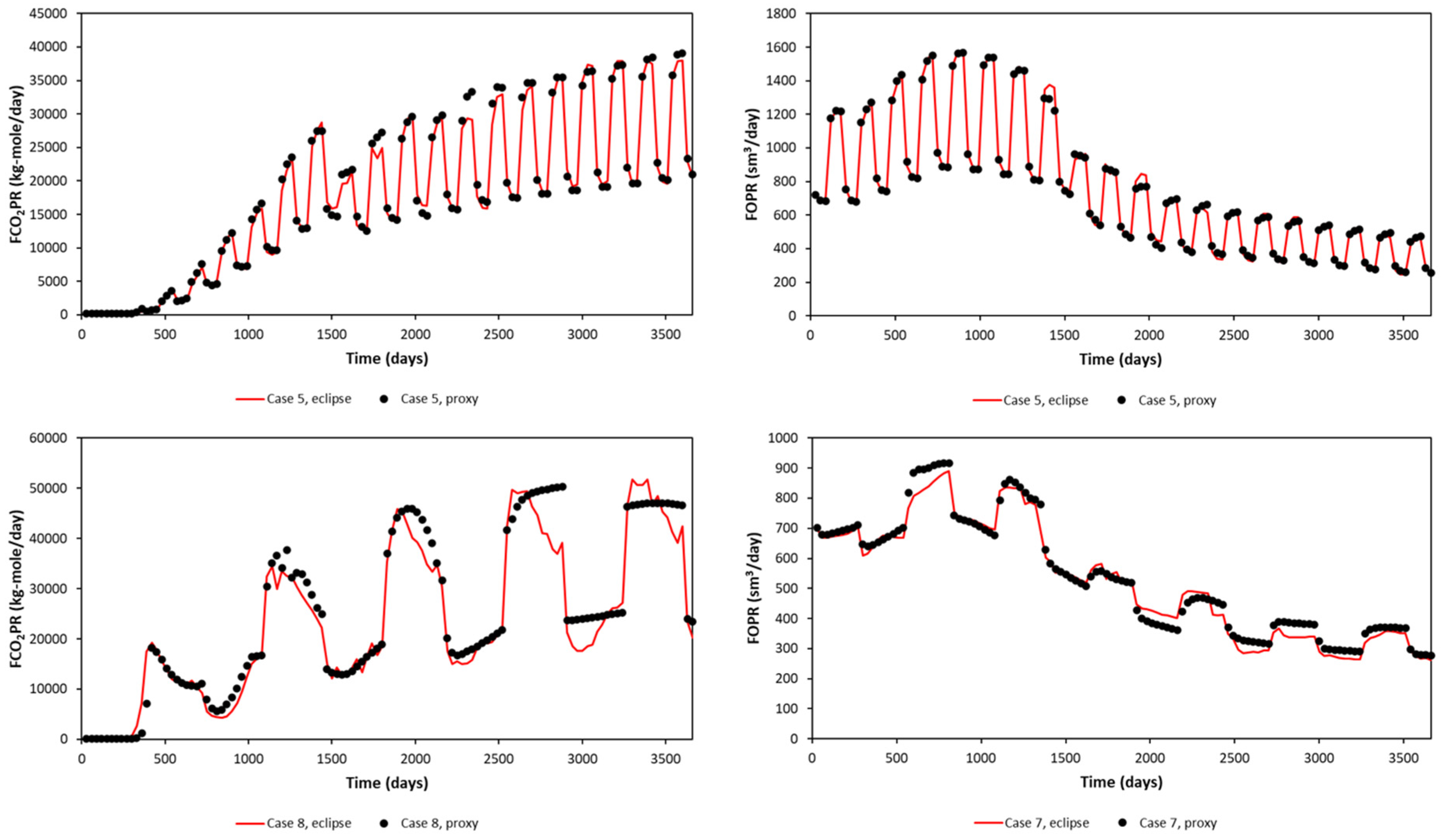
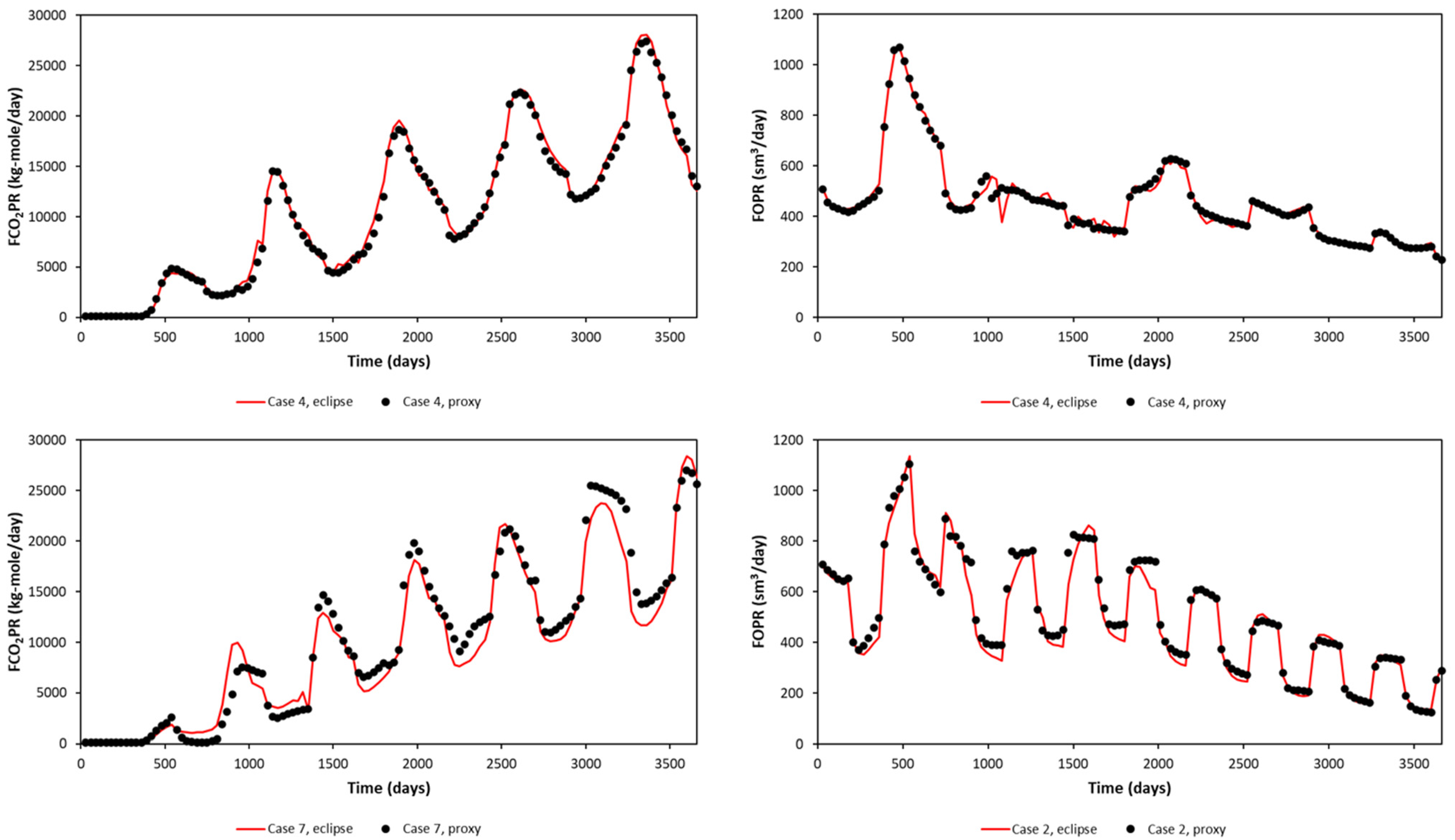
4.2. Data Preparation

Based on the formulation of the optimization problem, two simulation outputs will be learned by the proxy, i.e., FOPR and FCO2PR. These variables are available as output results of a simulation run. In addition, the half-cycle length, timestep, gas injection rate, and water injection rate are used as the proxy inputs. Normalization is performed to help the convergence of the ANN. Maximum–minimum normalization will be performed as:
x Norm = x x min x max x min

4.3. Proxy Building

The proxy can be developed properly only if the types of proxy built and data used are known. Failure to perform in sequence will cause an infinite loop between these three sections (problem formulation, model preparation, and proxy building) until the first two sections are determined. An overview that shows the outline of the study, performed with the available software and programming language, is shown in Figure 6.
WAG has distinct behavior. For a WAG ratio higher than 1, a sharp increase in production during the water injection phase is observed. When the WAG ratio is less than 1, an increase in production during the gas injection phase is noted. This distinct behavior is thus used as the base of building the proxy. The database is then split based on the injection phase. These concepts are applied to FCO2PR and FOPR proxies. For the Gullfaks model, a sharp production change is identified after 1 month, since the injection fluid (water or CO2) was changed, which can be observed as a delay compared to the Egg model. This results in proxy segmentations based on the injection phase.

4.4. Proxy Training and Validation

An optimization process was conducted to find the best topology of the ANN for every proxy segmentation. The optimized parameters were the learning rate, number of hidden layers, and number of nodes of each layer with an epoch of 100 with MSE (Equation (3)) used as the loss function. The optimum hyperparameters are then retrained with 1500 epochs to obtain their best performance. The detailed hyperparameters are listed in Table 3.
M S E = 1 n i = 1 n X i X i , p r e d i c t e d 2
It is essential to think of the behavior of the segments as a one proxy system. As one of the inputs is the result from the previous timestep, the value obtained from the proxy was used as the input value. The segments were then tested as parts of one proxy to verify its robustness. In lieu of relying on visual inspection, an error calculation was performed to quantify the robustness of the proxy model. For this reason, the average percentage relative error (%) was used. The equation is shown below.
APRE = X p r e d X r e a l X r e a l · 100

4.5. Blind Test

Following training, a blind test was performed on the proxy models. Here, 12 runs outside of the sampling from LHS were prepared. The same assessment as explained above was performed before the proxy model was used, where APRE was used as the error calculation to determine the performance.

4.6. Optimization Study

NSGA-II was employed in this study. It is worth mentioning that no optimization study was performed for the hyperparameters in our optimization algorithm. To perform this, a better understanding of how the NSGA- II function is built must be acquired. Other than that, the population size will be kept at 40. The number of generations for one study was set to 100, where ten new offsprings will be generated in each generation. The whole study will take more than 1000 proxy runs to be finished.

5. Results

5.1. Proxy Structure Results

Sampling was performed using Latin Hypercube Sampling (LHS). In total, 68 (Egg Model) and 97 (Gullfaks Model) runs were performed on the proxy training validation dataset. Eight samples, representative of the Latin Hypercube space, are included. This is based on a three-dimensional hypercube, which indicates eight edges based on the combination of extremes of the studied parameters.
The proxies are segmented into several parts. The distinct WAG behavior explained before is used as the base idea, then additional ideas are included to complement and give better proxy results. The first idea is to mimic the first-year behavior, which is unique compared to the others. For this part, the proxy is not differentiated based on its injection phase. The second idea is to build one proxy to mimic the performance of the first 5 years and another proxy to mimic the behavior from the 6th year to 10th year. The segmentation results for each model are listed below.
1.
Egg Model:
-
The base: both proxies (FOPR and FCO2PR) are segmented based on injection phase.
-
Timestep split: the proxy is then split again into 1st year, 2nd year–5th year, and 6th year–10th year.
2.
Gullfaks Model:
-
The base: both proxies (FOPR and FCO2PR) are segmented based on injection phase.
-
Half-cycle split: the base is then segmented based on low half-cycle lengths (3 and 6 months) and high half-cycle lengths (9 and 12 months).
-
Timestep split: the proxy is then split again into 1st year, 1st year–2.5th year, 2.5th year–5th year, 5th year–7.5th year, and 7.5th year–10th year.

5.2. Proxy Training, Validation, and Testing Results

As explained above, an optimization process was executed to find the best topology of the ANN for every segment. After that, an APRE analysis, shown in Table 4, was conducted for both models. An average 2% APRE with an error window less of than 10% range was the target.
A significant error can be seen in the maximum and minimum of FCO2PR. This is due to the error obtained at early times (first year), as the difference in small value leads to a significant error calculated in APRE term. Nevertheless, FCO2PT (Field CO2 Produced Total) should be the focus, as it will be used in the optimization study. The proxy and reservoir model results (selected randomly) are shown in Figure 7 for the Egg Model and Figure 8 for the Gullfaks Model.
After the training and validation, the proxy model was tested with the blind test data. Table 5 shows the APRE of the blind test results. The error window is about the same as the training validation dataset. A considerable difference is again observed in the F CO2PR maximum error. Observing the data for every timestep indicates that the error is due to the early time errors, the same as observed in the training validation phase.
A random blind test (upper) and the worst blind test (lower) in terms of FOPT and FCO2PT errors are plotted in Figure 9 for the Egg Model and Figure 10 for the Gullfaks Model. The blind-tested proxy is then ready to be used as a proxy to represent the reservoir model. An optimization study was then performed with this proxy model.

5.3. Optimization Study Results

NSGA-II was employed in this study. Forty pareto solutions from the Egg Model proxy and 32 pareto solutions from the Gullfaks Model proxy were obtained, as shown in Figure 11. As there are no objective functions that need to be prioritized, the middle point of the front or the value near the mean of all possible positions can be selected. From all Pareto solutions, the one that is selected is the one closest to the average values of both objective functions.
It is crucial to test the relative error between the solution and the actual reservoir model run result. The selected Pareto optimum is then tested using PETREL. All error results (between the proxy and reservoir model) are shown in Table 6. The results show a miniscule relative error for the selected cases.

6. Discussion

Each proxy model is case specific based on the data provided for its learning. This results in limitations of the proxy models; for example, they are not seen as one-size-fits-all solutions for optimization problems. In this work, the proxy models were created based on the discussed reservoir models. They do not have the ability to reflect the physical trends of other reservoir models. Hence, this, to a certain extent, limits their application. Additionally, the established proxy models are field based. This indicates that they are only able to depict the responses of the reservoir on the field scale, such as FOPR. These proxy models cannot predict any output on the grid and well scales. In this study, the methodology was illustrated without aiming to create a model that is a universal solution. Therefore, two proxy models that represent different reservoir models were built for solving the optimization problem in this study. One of the models (Egg Model) was modified to make both models similar in size for comparison purposes. A comparative study will be presented based on the steps of building the proxy model. Concerning this, it is important to note that this methodology was only tested with simulation data. Therefore, justification with real field data is recommended (when available) in future work to achieve higher maturity in terms of implementation.

6.1. Data Complexity

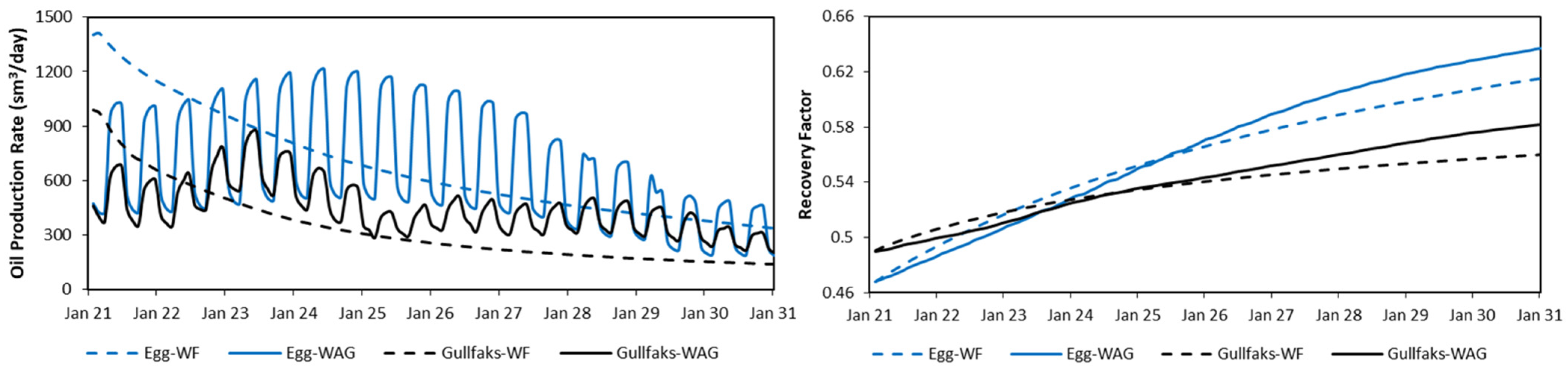
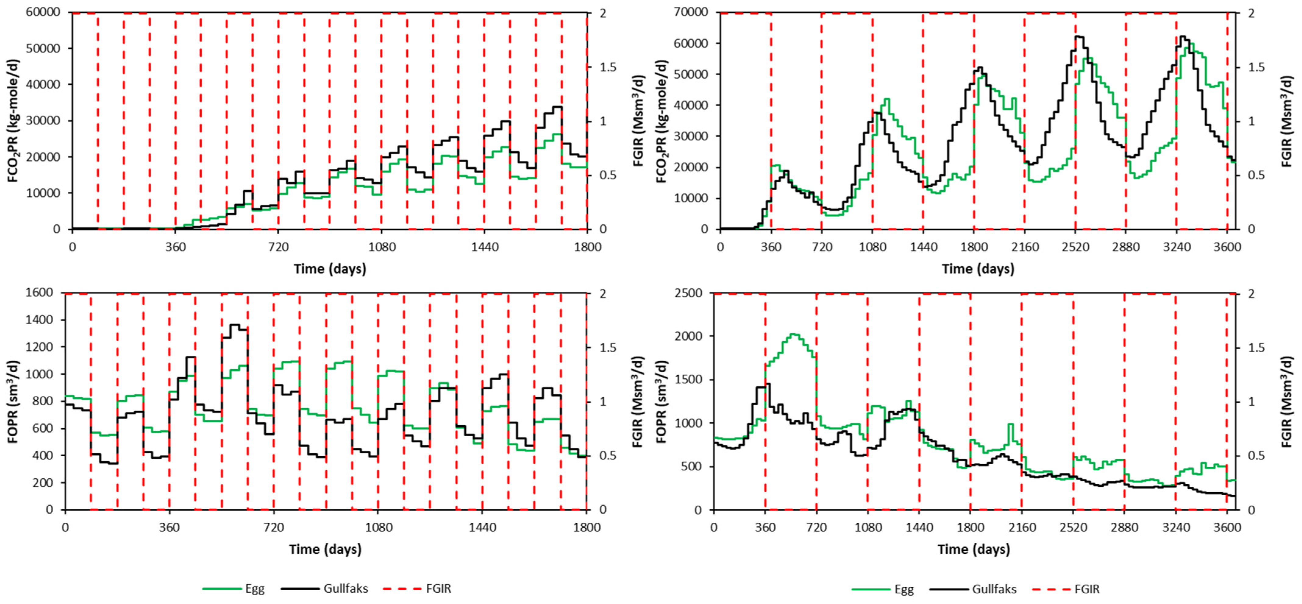
The rate response to the WAG injection phase for both models is shown in Figure 12. Two cases are presented. One is for a 90 day half-cycle length, 2 Msm3/d gas injection rate, and 3000 sm3/d water injection rate. This case is shown until 1800 days only. The other case is for a 360 day half-cycle length, 2 Msm3/d gas injection rate, and 9000 sm3/d water injection rate. These cases were run as training cases for both models, as one of Latin Hypercube edges.
Regarding FCO2PR behavior, a sharp increase in CO2 production can be seen for the 90 day half-cycle. However, in the case of the 360 day half-cycle for the Gullfaks model, there is a smooth transition rather than a sharp increase or drop in production behavior. This different behavior will be learned using the same proxy model if it is not segmented based on half-cycle length. From FOPR plots, higher production rates can be noticed compared to the base case shown in Figure 5.
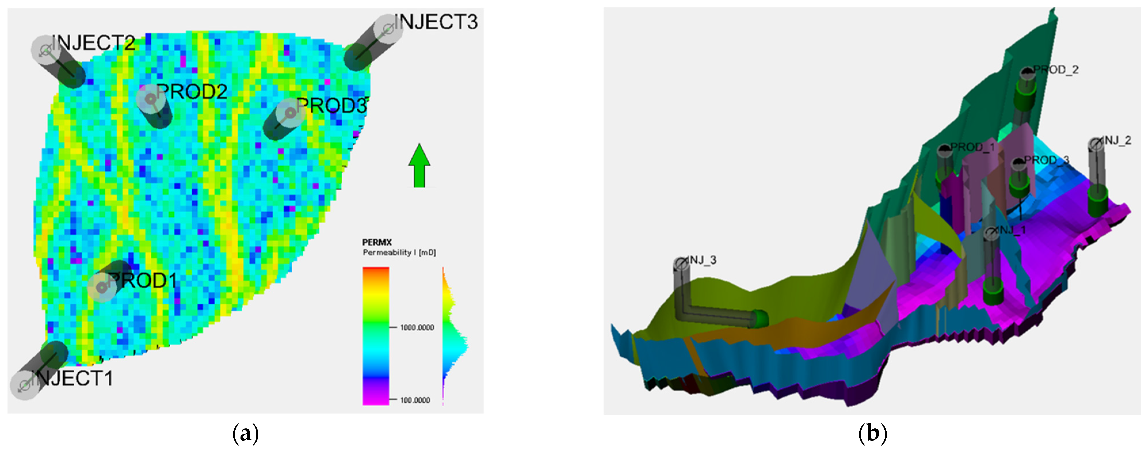
The difference in the responses of the two models is primarily due to different geological model and well placements. Other parameters such as fluid model, relative permeability relationships, and initialization are identical for both models. The complex behaviors were learned by the proxies built for the respective reservoir models.

6.2. Number of Samples Needed

It can be concluded that complexity aligns with the number of samples needed for developing the proxy. For the Egg Model, 68 samples are enough, while for the Gullfaks model, 97 samples are needed to develop the proxy model. The total time to run all samples is aligned with the number of samples needed. This phase is the most time-consuming part as both models need more than 9 h to complete all runs for the training validation dataset.
There is generally no stringent guide in deciding the exact number of samples used in building a proxy [29]. Adding extra runs means increasing the dimensionality, the amount of time to collect the data, and additional time needed for the algorithm to learn the data. Therefore, there is a trade-off to be considered when selecting the number of samples. To tackle this, segmentations were performed, which will be explained in the next section.

6.3. Proxy Model Development Process

To improve the robustness, segmenting the proxy was the first attempted method rather than increasing the number of samples. Segmenting the time into several parts shows the best improvement compared to other methods. The question that might arise is the number of segmentations needed. In this study, three segmentations were enough for the Egg model, but more than five were needed for the Gullfaks model.
Before assessing the proxy robustness, the computational time needed to build all the proxy segments was studied. Here, the time presented includes the database segmentation, topology optimization, re-learning of ANN with higher epoch, and running the whole training validation blind dataset using the proxy model. More data and segmentation will increase the amount of time needed. All proxy development statistics are tabulated in Table 7.

6.4. Proxy Robustness

In this study, an average APRE of less than 2% for the training validation phase was used as the target. Other than that, the error window should be in the range of 10%. These numbers are selected arbitrarily as the boundary for this study. Both proxy models must fulfill these criteria before being tested using the blind test dataset. A more profound assessment was also performed to determine the error variations for each training validation case.
Both models are assessed using the blind test as the final test to check the robustness. In general, both models have similar APRE values for both training, validation, and blind tests. The robustness of blind test was assessed in the same way as for the training and validation. It is observed in this study that when the proxy model meets the robustness criteria during the training and validation, it tends to show the same robustness during the blind test.

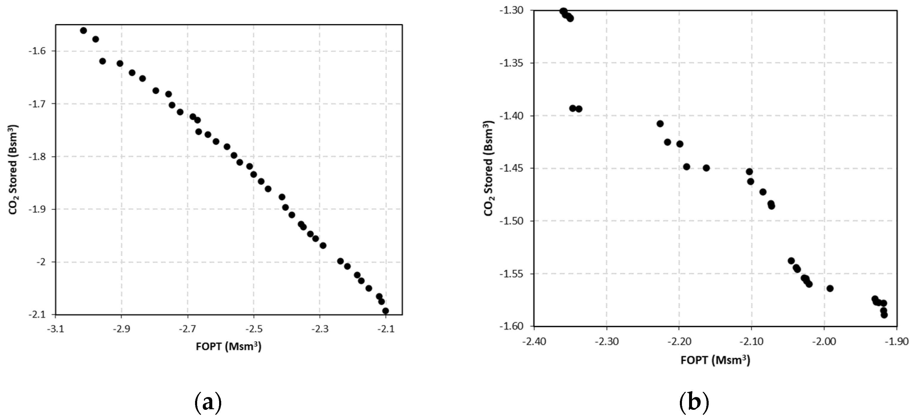
6.5. Optimization Results

Both proxy models need an almost equal amount of time to finish optimization. The difference between the proxy models in the time taken to finish a run is only 0.41 s. No hyperparameters were changed and the total generations used for both models were the same (100 generations).
The number of Pareto optima are different, where there are 40 Pareto optima in the Egg model and only 32 Pareto optima in the Gullfaks model. The Pareto front of the two models is different. Both models still have the same behavior. If the water injection rate is increased while the gas injection rate stays the same, the oil production will increase while the amount of CO2 stored in the reservoir will reduce. For the Egg model, this behavior is almost linear. However, for the Gullfaks model, it is not anywhere near linear. All statistics for the optimization process are tabulated in Table 8.

7. Conclusions

In this study, an advanced workflow was proposed for establishing proxy models de-voted to optimizing the WAG CO2 process. The proxy models were proven to be powerful modeling tools and can efficiently tackle the problems associated with conventional reservoir simulations, such as runtime and memory needed to store the results. In this context, the proxy models were built to mimic the oil production rate and CO2 production rate, where the Egg model was the simple reservoir model and the Gullfaks model was the complex reservoir model in this study. Several proxy segments were used to construct these proxy models. Each segment was made using an ANN. The robustness (as a whole proxy) was tested using APRE, both during training and validation and blind testing. The results can be improved by changing the ANN, the assessment of the proxy, or even the optimization algorithm. In addition, the following points can be highlighted.
  • A higher number of samples is needed for a more complex reservoir. For the Egg Model, 68 samples are enough, but for the Gullfaks model, 97 samples are required to develop an appropriate proxy model.
  • To obtain the maximum oil recovery for CO2-WAG study, a maximum gas injection rate with a minimum water injection rate is needed. This will, however, reduce the amount of CO2 stored in the reservoir. A linear relationship between water injection rate, total oil produced, and total CO2 stored can be observed in the simple reservoir model. The complex reservoir model shows the same trend, but the relationship is not linear. This is because of the reservoir heterogeneity that affects the sweep efficiency and the CO2 entrapment.

8. Future Recommendations

Based on this study, there are several recommendations that may be implemented in future work.
  • The workflow developed here can be employed as a good starting point to develop proxy models, for example, to be used in optimization studies.
  • A separate study regarding the amount of sampling and sampling method is recommended as there is no clear guideline on how the sampling must be performed.
  • APRE leads to positive and negative errors. This might lead to incorrect overall error values, and hence incorrect proxy robustness assessments. The AAPRE (average absolute percentage relative error) might be more suitable to assess the performance of the proxy, as this will remove the possibility of the negative errors being nullified by other positive value errors.

Author Contributions

Conceptualization, D.A.M.M., A.J.G., C.S.W.N. and M.N.A.; methodology, D.A.M.M., A.J.G., C.S.W.N. and M.N.A.; software, D.A.M.M.; formal analysis, D.A.M.M.; investigation, D.A.M.M.; data curation, D.A.M.M.; writing—original draft preparation, D.A.M.M.; writing—review and editing, A.J.G., C.S.W.N. and M.N.A.; visualization, D.A.M.M.; supervision, A.J.G., C.S.W.N. and M.N.A. All authors have read and agreed to the published version of the manuscript.

Funding

This research received no external funding.

Data Availability Statement

All results are available on GitHub: https://github.com/aqnanp/CO2WAG-Proxy-Study (accessed on 10 October 2022).

Acknowledgments

This research is part of the activities of CEORS Gemini- Center (CO2 Enhanced Oil Recovery and Storage), a strategic cooperation between NTNU and SINTEF (https://www.ntnu.edu/ceors, accessed on 18 July 2022). We would like to thank Curtis Hays Whitson for guidance in PVT modeling and Whitson AS for the Advanced PVT Course that aided in the PVT modeling in this study.

Conflicts of Interest

The authors declare no conflict of interest.

References

  1. International Energy Agency. Global Energy Review 2021; International Energy Agency: Paris, France, 2021. [Google Scholar]
  2. OECD. OECD Economic Outlook; Issue 1; OECD: Paris, France, 2021; Volume 2021. [Google Scholar]
  3. International Energy Agency. Oil 2021; International Energy Agency: Paris, France, 2021. [Google Scholar]
  4. IRENA. Renewable Capacity Statistics 2021; IRENA: Masdar City, United Arab Emirates, 2021. [Google Scholar]
  5. World Bank. State and Trends of Carbon Pricing 2020; World Bank: Washington, DC, USA, 2020. [Google Scholar]
  6. Equinor. So Why Is the New Johan Sverdrup Field so Important? Available online: https://www.equinor.com/en/magazine/why-is-johan-sverdrup-so-important.html (accessed on 16 June 2021).
  7. Jacobs, T. CO2 EOR Could Be Industry’s Key to a Sustainable Future or Its Biggest Missed Opportunity. J. Pet. Technol. 2020, 72, 17–20. [Google Scholar] [CrossRef]
  8. Jarrell, P.M.; Fox, C.E.; Stein, M.H.; Webb, S.L. Practical Aspects of CO2 Flooding; Society of Petroleum Engineers: Richardson, TX, USA, 2002. [Google Scholar]
  9. Christensen, J.R.; Stenby, E.H.; Skauge, A. Review of WAG Field Experience. SPE Reserv. Eval. Eng. 2001, 4, 97–106. [Google Scholar] [CrossRef]
  10. Zubarev, D.I. Pros and Cons of Applying Proxy-Models as a Substitute for Full Reservoir Simulations. In Proceedings of the Proceedings—SPE Annual Technical Conference and Exhibition, New Orleans, LA, USA, 4–7 October 2009; Volume 5. [Google Scholar]
  11. Matthew, A. Proxy Modeling for CO2-EOR Design Study: Water Alternating Gas and Storage. Master’s Thesis, Norwegian University of Science and Technology, Trondheim, Norway, 2021. [Google Scholar]
  12. Gholami, V. On the Optimization of CO2-EOR Process Using Surrogate Reservoir Model. Ph.D. Thesis, West Virginia University, Morgantown, WV, USA, 2014. [Google Scholar]
  13. Amini, S. Developing a Grid-Based Surr Eloping a Grid-Based Surrogate Reser Ogate Reservoir Model Using Oir Model Using Artificial Intelligence. Ph.D. Thesis, West Virginia University, Morgantown, WV, USA, 2015. [Google Scholar]
  14. Chaki, S.; Zagayevskiy, Y.; Shi, X.; Wong, T.; Noor, Z. Machine Learning for Proxy Modeling of Dynamic Reservoir Systems: Deep Neural Network DNN and Recurrent Neural Network RNN Applications. In Proceedings of the International Petroleum Technology Conference 2020, IPTC 2020, Dhahran, Kingdom of Saudi Arabia, 13–15 January 2020. [Google Scholar]
  15. Nait Amar, M.; Jahanbani Ghahfarokhi, A.; Ng, C.S.W.; Zeraibi, N. Optimization of WAG in Real Geological Field Using Rigorous Soft Computing Techniques and Nature-Inspired Algorithms. J. Pet. Sci. Eng. 2021, 206, 109038. [Google Scholar] [CrossRef]
  16. Nait Amar, M.; Zeraibi, N.; Jahanbani Ghahfarokhi, A. Applying Hybrid Support Vector Regression and Genetic Algorithm to Water Alternating CO2 Gas EOR. Greenh. Gases Sci. Technol. 2020, 10, 613–630. [Google Scholar] [CrossRef]
  17. Ng, C.S.W.; Jahanbani Ghahfarokhi, A.; Nait Amar, M.; Torsæter, O. Smart Proxy Modeling of a Fractured Reservoir Model for Production Optimization: Implementation of Metaheuristic Algorithm and Probabilistic Application. Nat. Resour. Res. 2021, 30, 2431–2462. [Google Scholar] [CrossRef]
  18. Ng, C.S.W.; Jahanbani Ghahfarokhi, A.; Nait Amar, M. Application of Nature-Inspired Algorithms and Artificial Neural Network in Waterflooding Well Control Optimization. J. Pet. Explor. Prod. Technol. 2021, 11, 3103–3127. [Google Scholar] [CrossRef]
  19. Ng, C.S.W.; Djema, H.; Nait Amar, M.; Jahanbani Ghahfarokhi, A. Modeling Interfacial Tension of the Hydrogen-Brine System Using Robust Machine Learning Techniques: Implication for Underground Hydrogen Storage. Int. J. Hydrogen Energy 2022, 47, 39595–39605. [Google Scholar] [CrossRef]
  20. Nait Amar, M.; Jahanbani Ghahfarokhi, A.; Zeraibi, N. Predicting Thermal Conductivity of Carbon Dioxide Using Group of Data-Driven Models. J. Taiwan Inst. Chem. Eng. 2020, 113, 165–177. [Google Scholar] [CrossRef]
  21. Salehian, M.; Haghighat Sefat, M.; Muradov, K. Multi-Solution Well Placement Optimization Using Ensemble Learning of Surrogate Models. J. Pet. Sci. Eng. 2022, 210, 110076. [Google Scholar] [CrossRef]
  22. Ng, C.S.W.; Jahanbani Ghahfarokhi, A. Adaptive Proxy-Based Robust Production Optimization with Multilayer Perceptron. Appl. Comput. Geosci. 2022, 16, 100103. [Google Scholar] [CrossRef]
  23. Blank, J.; Deb, K. Pymoo: Multi-Objective Optimization in Python. IEEE Access 2020, 8, 89497–89509. [Google Scholar] [CrossRef]
  24. Kumar, H.; Yadav, S.P. Fuzzy Rule-Based Reliability Analysis Using NSGA-II. Int. J. Syst. Assur. Eng. Manag. 2019, 10, 953–972. [Google Scholar] [CrossRef]
  25. Jansen, J.D.; Fonseca, R.M.; Kahrobaei, S.; Siraj, M.M.; Van Essen, G.M.; Van den Hof, P.M.J. The Egg Model—A Geological Ensemble for Reservoir Simulation. Geosci. Data J. 2014, 1, 192–195. [Google Scholar] [CrossRef]
  26. Negahban, S.; Pedersen, K.S.; Baisoni, M.A.; Sah, P.; Azeem, J. An EoS Model for a Middle East Reservoir Fluid with an Extensive EOR PVT Data Material. In Proceedings of the Society of Petroleum Engineers—14th Abu Dhabi International Petroleum Exhibition and Conference 2010, ADIPEC 2010, Abu Dhabi, United Arab Emirates, 1–4 November 2010; Volume 1. [Google Scholar]
  27. Al Adasani, A.; Bai, B. Analysis of EOR Projects and Updated Screening Criteria. J. Pet. Sci. Eng. 2011, 79, 10–24. [Google Scholar] [CrossRef]
  28. McKay, M.D.; Beckman, R.J.; Conover, W.J. A Comparison of Three Methods for Selecting Values of Input Variables in the Analysis of Output from a Computer Code. Technometrics 1979, 21, 239–245. [Google Scholar] [CrossRef]
  29. Shahkarami, A.; Mohaghegh, S. Applications of Smart Proxies for Subsurface Modeling. Pet. Explor. Dev. 2020, 47, 400–412. [Google Scholar] [CrossRef]
Figure 1. Workflow of proxy modeling [10].
Energies 16 03337 g001
Figure 2. Main ANN structure.
Energies 16 03337 g002
Figure 3. Model illustration, faults, well locations, and perforation zones for (a) the Egg Model and (b) the Gullfaks Model.
Energies 16 03337 g003
Figure 4. EOS tuning results for the PVT data used.
Energies 16 03337 g004
Figure 5. Test results of the CO2-WAG feasibility study for both models.
Energies 16 03337 g005
Figure 6. Workflow of proxy building, the optimization study, and the software involved in this study.
Energies 16 03337 g006
Figure 7. Proxy results and comparison with the reservoir simulation output, sampled cases show different injection patterns (3 months, 6 months, and 12 months) (Egg Model).
Energies 16 03337 g007aEnergies 16 03337 g007b
Figure 8. Proxy results and comparison with the reservoir simulation output, sampled cases show different injection patterns (3 months, 6 months, and 12 months) (Gullfaks Model).
Energies 16 03337 g008
Figure 9. Proxy results and comparison with the reservoir simulation output (Egg Model), blind test.
Energies 16 03337 g009
Figure 10. Proxy results and comparison with the reservoir simulation output (Gullfaks Model), blind test.
Energies 16 03337 g010
Figure 11. Pareto front for: (a) the Egg Model and (b) the Gullfaks Model.
Energies 16 03337 g011
Figure 12. Differences between the Egg Model and the Gullfaks Model regarding rate response to the WAG injection phase (left: 90 day half-cycle, right: 360 day half-cycle).
Energies 16 03337 g012
Table 1. Overview of the two reservoir models in this study.
ParameterEgg ModelGullfaks Model
PermeabilityChannel distributionHeterogeneous
PorosityHomogeneousHeterogeneous
Faults014
FluidFrom SPE136530From SPE136530
TransmissibilityNo multiplierHeterogeneous multiplier
Relative permeabilitySand presetSand preset
Grid systemCartesianCornerpoint
Grid sizeHomogeneousHeterogeneous
Initial condition320 bar, 120.85 °C, 1850 m320 bar, 120.85 °C, 1850 m
WellsThree injectors, three producersThree injectors, three producers
PerforationsThroughout all layersDifferent for each well
Table 2. Depletion scenario parameters and results after depletion for both models.
ParameterEgg ModelGullfaks Model
Injection rate2000 sm3/day/well2000 sm3/day/well
Production rate limit2000 sm3/day/well2000 sm3/day/well
Start of depletion1 January 20131 January 2013
End of depletion1 January 20211 January 2021
STOOIP16.55 Msm317.24 Msm3
STOIP (2021)8.94 Msm38.90 Msm3
RF46.0%48.4%
Pavg (2021)254.9 bar264.3 bar
Table 3. Hyperparameters in ANN design.
ParameterValue
Learning functionAdam
Learning rate10−6–10−2
Number of hidden layers1–3
Number of nodes2–20
Activation functionrelu
Batch size64
Dropout-
Training ratio75
Validation ratio25
Loss functionMSE
Epochs100, then 1500
Table 4. APRE statistics of each model for training and validation phases.
ParameterAPRE, Egg Model (%)APRE, Gullfaks Model (%)
MinAverageMaxMinAverageMax
FOPR−2.307−0.1293.227−2.3640.0421.443
FCO2PR−9.8820.84210.962−2.8711.27011.166
FOPT−2.435−0.2682.449−2.533−0.1251.429
FCO2PT−3.2521.0526.114−6.048−0.9092.778
Table 5. APRE statistics of each model for the blind test phase.
ParameterAPRE, Egg Model (%)APRE, Gullfaks Model (%)
MinAverageMaxMinAverageMax
FOPR−1.0780.6462.85−0.70.5113.93
FCO2PR−3.5382.94412.433−1.8232.00610.055
FOPT−1.5750.1682.162−0.7280.1943.405
FCO2PT−1.7831.745.81−2.191−0.0715.612
Table 6. Error analysis (between the proxy model and the reservoir simulation results).
ParameterEgg ModelGullfaks Model
PETRELProxyRelative Error (%)PETRELProxyRelative Error (%)
FOPR *--0.26--1.04
FOPT (Msm3) 2.492.511.052.082.11.19
FCO2PR *--1.23--0.45
FCO2PT (Msm3)78.8479.430.7595.9194.83−1.12
* The relative error shows the average error between the simulation and proxy results for each timestep. The values of FOPR and FCO2PR are not specified as they comprise a set of data points.
Table 7. Proxy development statistics.
Process EggGullfaks
SamplingLHS6897
Sampling time9 h 43 m12 h 35 m
Run time per case9 m 25 s8 m 45 s
Memory space per case97 MB85 MB
Proxy DevelopmentFOPR2 ANNs8 ANNs
FCO2PR5 ANNs9 ANNs
Total time needed1 h 23 m2 h 49 m
Proxy PerformanceRun time8.75 s9.16 s
Memory space14 KB13 KB
Table 8. Optimization study statistics.
EggGullfaks
Pareto optima4032
Time needed2 h 25 m2 h 23 m
Runs needed10301030
Eclipse equivalent time6 d 17 h 39 m6 d 5 h 38 m
ResultsHalf-cycle (months)3–63–9
Gas rate (Msm3/d)1.98–21.95–2
Water rate (sm3/d)3000–90003000–9000
Disclaimer/Publisher’s Note: The statements, opinions and data contained in all publications are solely those of the individual author(s) and contributor(s) and not of MDPI and/or the editor(s). MDPI and/or the editor(s) disclaim responsibility for any injury to people or property resulting from any ideas, methods, instructions or products referred to in the content.

