
Water System Safety Analysis Model

Department of Water Supply and Sewerage Systems, Faculty of Civil, Environmental Engineering and Architecture, Rzeszow University of Technology, Al. Powstancow Warszawy 6, 35-959 Rzeszow, Poland
*
Author to whom correspondence should be addressed.
Energies 2023, 16(6), 2809; https://0-doi-org.brum.beds.ac.uk/10.3390/en16062809
Submission received: 15 February 2023
/
Revised: 10 March 2023
/
Accepted: 15 March 2023
/
Published: 17 March 2023
(This article belongs to the Special Issue The Energy Water Nexus)
Abstract
:The operation of a water supply system (WSS) is inextricably linked with the possibility of different types of failure. It is very common for these failures to be random in nature. The results of reliability studies carried out in many water supply systems revealed, for example, the possibility of incidental water pollution, power supply issues, failure in machinery, damage to water plants, or natural disasters. As a result of the WSS failure, we deal with a state of threat to safety (TSS) or a state of loss of safety (LSS). Using Markov processes, we developed a failure model of the WSS to determine the possibility that the system may find itself in different states of safety. As a result, a mathematical model using Markov processes has been proposed for each of these distinct states of safety (complete safety state—CSS; threat to safety state—TSS; and loss of safety state—LSS). The proposed approach in the water supply system will limit emergency states by optimizing working and repair times. Reducing losses in the water supply system is crucial to reduce and optimize energy consumption for water production and distribution.
1. Introduction
Water, electricity, gas, and other supply systems play a strategic role in the security of facilities and installations with respect to the water–energy nexus. According to the 7th goal of the 2030 Agenda [1] for Sustainable Development, the place of living is safe, resilient, and sustainable, with general access to affordable, reliable, and sustainable energy. Therefore, regulations and guidelines include these systems in the so-called critical infrastructures. The safety of the water supply system (WSS) is the ability of the system to perform its functions in a safe manner to itself and its environment, despite the occurrence of various types of adverse events. The safety of the water supply system is measured by the probability of staying in a safe operating configuration when faced with an adverse (cause) hazardous event (cause). Losing safe functioning may impact the system itself, its environment, and/or the health or life of consumers (effects) [2].
UN global development program has recognized the access right for all to safe drinking water and sanitation, as cited in the resolution 64/292 of the General Assembly and the Human Rights Council states that the right to access safe and clean drinking water and sanitation is a human right necessary for the full enjoyment of life and the enjoyment of all human rights [3]. Resolution No. 1693/2009 of the Parliamentary Assembly of the Council of Europe contained a provision that access to water must be recognized as a fundamental human right because water is necessary for life on Earth and is a common good, belonging to all mankind [4].
A water utility should provide recipients with water of appropriate quality, in the right quantity, and under the appropriate pressure, and, according to the Regulation on the quality of water intended for human consumption, it should be free of pathogenic microorganisms and parasites that could pose a threat to human health, or any substances in concentration that are potentially harmful to human health and must not indicate aggressive corrosive properties. Further, it must meet the microbiological and chemical requirements specified in the Regulation [5,6].
In recent years, there has been an increase in safety-related risks, such as large-scale power failures or blackouts resulting from the generalized use of ICT and the systemic connectivity of different critical infrastructures [7]. The risk of other undesirable events that may result in a failure of the water supply system makes it necessary to develop alternative solutions to supply people with drinking water in crisis situations [8,9]. Water supply systems are an important element of critical infrastructure. They should be subject to increasingly restrictive requirements in terms of resilience and business continuity, especially in crisis situations, including blackouts [10,11].
There are several undesirable events associated with the daily operation of the water supply system (WSS), including secondary contamination of drinking water in the distribution subsystem, breaks in the water supply, or drops in water pressure [12,13]. Water supply systems are characterized by continuous work, and due to the specific requirements associated with them, they must be highly reliable, both operationally and in terms of safety, particularly in terms of the safety of water consumers [14,15,16]. As one of its characteristics, the WSS is capable of changing its properties, which have a significant impact on the reliability and safety of the system [17].
A WSS can progress from complete capability (reliability and safety) to partial incapability (threat to safety), up to complete incapability, resulting in a loss of the system safety (threat to water consumers), depending on the type, character, and magnitude of the failure [18,19,20]. To determine the probability that a particular state will occur, an analysis using the Markov process method was conducted, whereby the reliability features of WSSs are represented using the so-called graph of states [21,22]. As a result of this method, it is possible to model the reliability of a system’s operation and safety over time [23]. In a Markov process, the probability of each event depends only on the result of a previous event (this is a random process without memory) [24]. The main purpose of this work is to perform a safety analysis of the WSS, implementing Markov processes. In order to reduce energy consumption for water production, e.g., pumping, a detailed analysis of safety conditions through the optimization of working and repair times is crucial. In the same way, the costs that are incurred by companies through water losses are examined. This is very significant in times of energy crisis.
2. Identification of System Safety States
Water supply systems that are the subject of interest in this paper are systems of a special type. Subsequently, they are characterized by dynamics and considerable inertia, and they are spatially extended. Such systems can be in various operational states [25,26]. These states, from the point of view of safety, can be classified into two sets: safe states (no damage) and unsafe states (loss of safety). From the point of view of reliability, these states can be classified into fitness and unfitness. Additional specific states of the system will also be considered. That is, “the state of emergency” [27]. The possibility of a quantitative description of this state was of interest to the authors [28,29]. The set of internal properties, defined by the interrelationship of the processes taking place in its subsystems, is defined as the state of the system at time t [5].
The condition is a set of properties that determines its ability to perform operational tasks. The state of threat to the system is characterized by destructive processes that occur during its operation [22,30,31]. It changes its operating characteristics, despite the fact that the system’s functional capabilities are maintained [32,33]. The failure condition is characterized by the inability to meet reliability requirements, i.e., provide drinking water in the right quantity and quality, under the required pressure, at any time convenient to the consumer, and an acceptable price [34]. Unfitness can be both reversible and irreversible. It is characterized by the fact that the system loses its ability to function fully or partially [35,36]. The reversibility of this condition is that the system may be fully operational after repair. When analyzing the system in terms of safety, the following states were additionally defined:
- Safety state (reliability)—CSS;
- Under threat—TSS;
And failure status:
- Loss (unreliability) of safety—LSS.
In work [36] for WSS, these states were defined as follows:
- CSS—the condition in which the system performs its functions in accordance with the applicable legal regulations and the expectations of water consumers in terms of the volume of production of drinking water (nominal water production efficiency is defined as Qn ≥ Qdmax) and quality (water meets the requirements of the applicable regulation). Emergency events may occur in the system’s operation, but the related losses C do not affect the system’s viability (they are negligible). It can be assumed that the relative value of the losses is equal to zero (C = 0). In terms of the safety of the water supply, the system meets the requirements for consumers but also does not pose a threat to the environment and other technical infrastructure—the tolerable state;
- TSS—a condition characterized by short-term disturbances in system operation: The daily production of water decreases (0.3 Qdmax ≤ Qn < Qdmax), or there are interruptions in its supply lasting up to 24 h (domino effect). The effects of the disturbances are greater than zero but less than or equal to the adopted limit values of Cgr, related to interruptions in water supply and threats to water consumers (possible exceedances of the normative values for the physicochemical parameters of water quality). If it is assumed that the relative value of the limit loss is equal to one, then 0 < C ≤ 1. In the aspect of safety, there is the so-called threat to water supplies to consumers or the environment (e.g., excessive water abstraction, leakage of chemicals) or other technical infrastructure (e.g., road washing)—the controlled state;
- LSS—a state in which the WSS does not fulfill its functions (Qn < 0.3 Qdmax) or water supply interruptions last longer than 24 h for individual housing estates, districts, or parts of the city. Consumers are exposed to the consumption of poor-quality water (exceeding the normative values for microbiological and (or) physicochemical indicators). Water quality poses a threat to the health or life of consumers: C ≥ Cgr = 1—the unacceptable state.
In terms of safety, there has been a loss of water supply safety—the system is not safe for the environment and other technical infrastructure.
- The variable X characterizes the system in terms of specific features of the system and their safety requirements;
- The Y variable characterizes the system in terms of system safety.
The variables X and Y can take the following values:
- X = 1 when all features of the system meet the safety requirements;
- X = 0 when at least one feature of the system does not meet the safety requirements;
- Y = 1 when there is no loss of system safety (tolerated or controlled state);
- Y = 0 when there is a loss of system safety (an unacceptable state).
Probabilities P(X) and P(Y|X) are assumed to be given. Therefore, the total probability is [28,29,38]:
P(X∧Y) = P(X) · P(Y|X),
Each of the variables X and Y describes two states of the system. Consequently, the system at time t may be in the following states [28,29,38]:
- X = 1 and Y = 1—CSS, the safety reliability state, which means that all features of the system meet the specified safety requirements of the system and there is no loss of safety. The probability of the condition occurring is:
P(CSS) = P(X = 1 ∧ Y = 1) = P(X = 1) · P(Y = 1|X = 1),
- The probability of safety is:
- X = 1 and Y = O—TSS1, the state that can occur theoretically. There has been a loss of safety in the system, but some features are within acceptable limits. The probability of the condition occurring is:
- X = 0 and Y = 1—TSS2, state of the safety emergency. At least one feature of the system does not meet the safety requirements, but there is no safety failure. The probability of the condition occurring is:
- X = 0 and Y = 0—state of safety unreliability LSS. One or more features of the system do not meet the safety requirements, and there is a safety failure.
The probability of the condition occurring is:
3. Methodology
Markov processes can also be used to model the reliability and safety of WSS. Detailed models in this regard can be found, among others, in the works [23,36].
In the analysis carried out by the Markov processes, we have the so-called state change graph. The use of Markov processes in safety analysis allows modeling the strategy of the system operation and the process of damage/renewal.
The equation should be solved with the following initial condition:
This way, the probability values of individual states are obtained. The transition matrix is as follows:
The development of the Markovian WSS safety model consisted of defining operational states, determining the transition matrix, and determining the initial distribution. WSS reliability analyses of the WSS proved that the working times between failure and recovery have exponential distributions. Thus, it is possible to construct a model of the functioning of the WSS based on the Markov process. Depending on the degree of susceptibility to the threat of the system and the protection of consumers against adverse events, five models have been proposed in [37], which show various possibilities of transition between defined operating states. For the models adopted in this way, Markov chains were used to determine individual stationary values of the probability of occurrence of individual operational states [36,40].
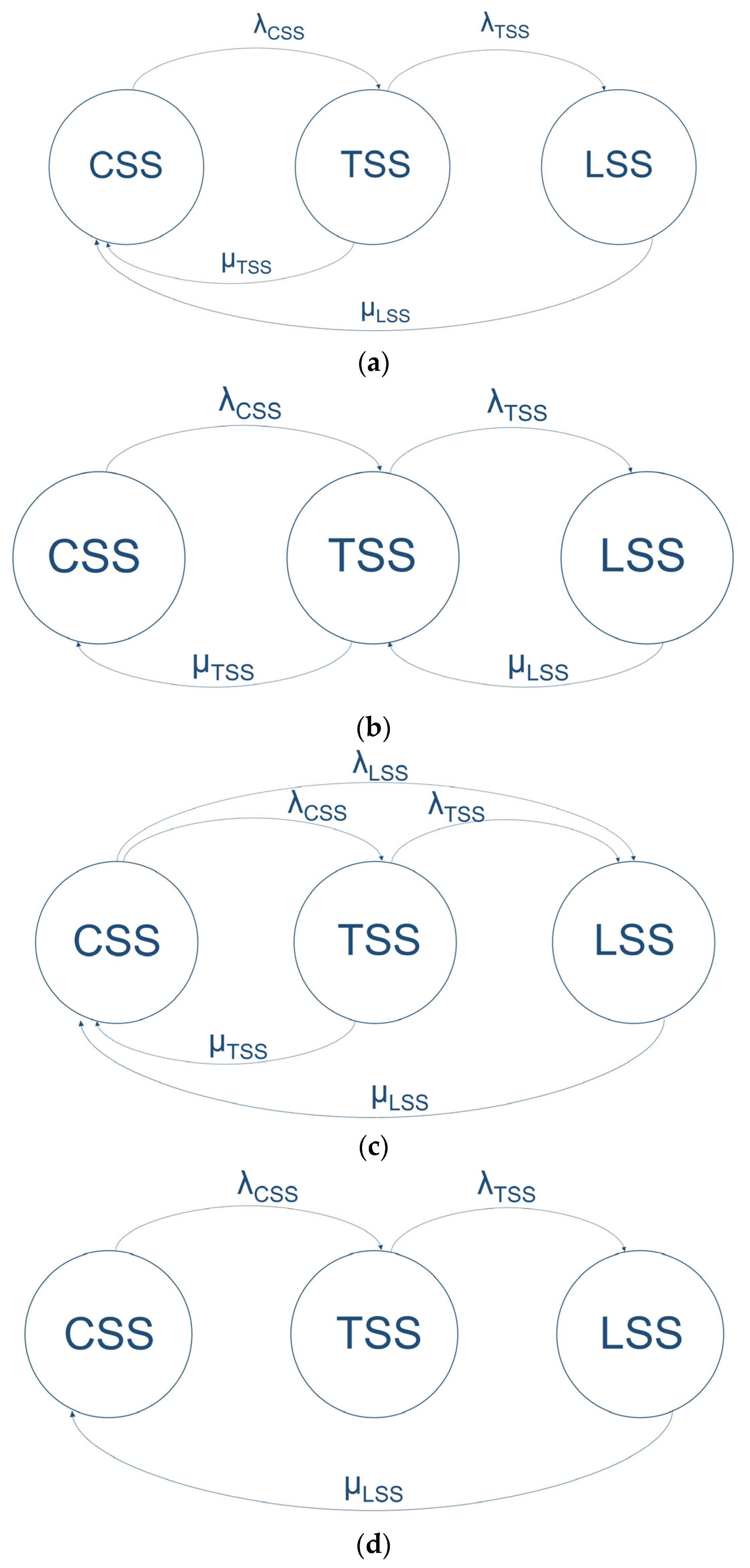
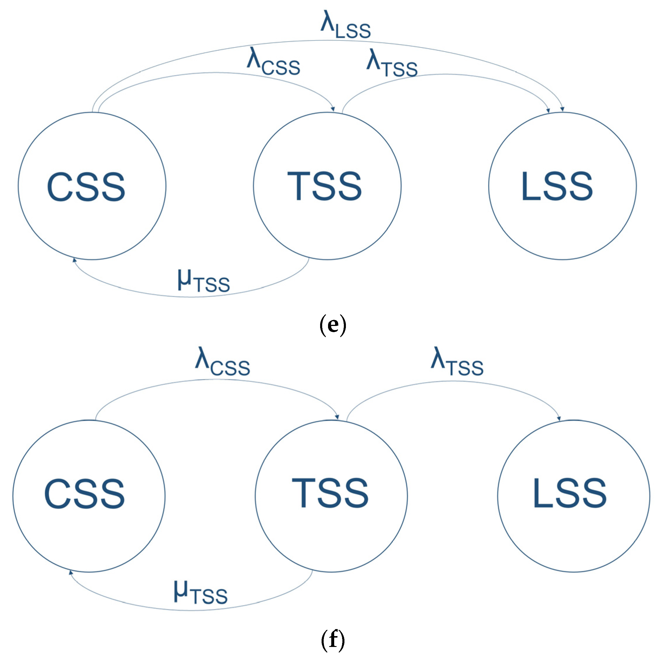
Figure 1 presents variants of the transition possibilities among the safety states of the WSS.
The model presented in Figure 1a assumed the possibility of developing an emergency, which is always preceded by an initiating event. The system may return to the CSS state as a result of the protection system. The model in Figure 1b took into account the possibility of removing the threat with the intensity transition of μTSS as a result of the operation of the protective barriers in the event of a threat occurrence. The transition of the system to the state of full operability; that is, the return from LSS to CSS, is always preceded by the TSS transition state, with the intensity transition of μLSS. The model assumed that it is possible to repair the system partially, i.e., to put it into operation conditionally, e.g., water supplied to some recipients with reduced pressure or the possibility of drinking water after boiling. This is the so-called conditional operation of the system until complete repair when the system goes to a state of full operability with the intensity transition of μTSS. Figure 1d characterizes the low-level protection model and standard water quality monitoring according to the current regulations. This model presents a situation in which, during the development of a crisis, there is no return from state TSS to state CSS, and the so-called domino effect occurs. Only when LSS arises is there a possibility to counter the threat and to return directly to the state TSS. The model in Figure 1e took into account the possibility of removing the threat of the transition intensity μTSS during the operation of the system. In the proposed model, there is a possibility of a direct transition from CSS to LSS state through sudden catastrophic events, such as pollution of water intakes connected with serious failures that cannot be reduced by the treatment process, such as long-lasting lack of power supply or failure in the strategic pipeline. The model in Figure 1f assumed that the failure situation develops with time and is always proceeded by the initiating event. In this case, the state CSS can contribute to the occurrence of a catastrophic event, but at the same time, as a result of the protection system, the system can return to the state CSS. As with model E, there is no possibility to counter LSS with the suitable μLSS. If the LSS state occurs immediately, it will depend on the type of system, treatment technology, repair and monitoring system, the efficiency and number of repair brigades, or the use of modern technologies. If we are able to react quickly to the LSS state, we go straight to the CSS state. In the case of a small system with a small number of brigades, the repair will be carried out in stages, and therefore slower, so indirectly the TSS state can occur, e.g., not a complete lack of water, but the need to boil water or water supply under reduced pressure.
The model shown in Figure 1c was selected. The model took into account the multistate of the system, as well as the occurrence of the so-called evaporation of the emergency state with the intensity of transitions μTSS during the operation of the WSS (e.g., timely correction of the water treatment process, the inclusion of alternative technologies, etc.). In this type of model, there is a possibility of a direct transition from CSS to LSS (emergency—catastrophic, e.g., contamination of water intakes related to serious accidents that the treatment process cannot reduce; flooding of the area of WSS; failure of a strategic pipeline; long-term total lack of power supply), as well as the possibility of vaporization of the LSS state with the appropriate intensity of the transitions. It should be noted that the intensity of transitions λLSS is associated with sudden events, and λTSS with the scenario of developing during a catastrophic situation (Domino effect, cascade failures) [41,42,43]. For the model defined this way, the following assumptions were made [28,29,38,39]:
- The occurrence of each condition is a random event; the transition probability corresponding to the individual states is: PCSS(t), PTSS(t), PLSS(t);
- The system can only be in one of the distinguished states at a time;
- At time t = 0, the subsystem is in the CSS state;
- Transition times between individual states have exponential distributions;
- Failure rate (or failure frequency) and repair parameter are, respectively, λ, μ;
- The graph directed from CSS to TSS and LSS to TSS means the occurrence of an emergency event with the probability λCSSΔt and λTSSΔt in the time interval Δt; the graph directed from LSS to TSS and TSS to CSS shows the system renewal process of the system with probability μ1Δt and μ2Δt over the time interval Δt;
The system of Kolmogorov differential equations based on formula (7) takes the following form [8,9,28]:
At time t = 0, the system is in CSS, which means that:
For stationary conditions, i.e., t → ∞ [28]:
4. Research Object
The source of water for the water treatment plant (WTP) is surface water. In the 1990s, the facility was modernized, introducing preliminary ozonation of raw water. The total production capacity of the WTP is Qmaxd = 84,000 m3⋅d−1. The WTP consists of two independent water treatment plants (WTPI and WTPII), located in one area, with a common intake.
The current possibilities for emergency water supply to the city, taking into account all available water sources, are as follows:
- Water stored in 18 equalizing reservoirs within the water supply network, with a total capacity of 35,300 m3;
- One hundred and seventy-nine emergency public wells with a total capacity of 689.4 m3⋅d−1, giving a total of 35,222 m3·d−1.
At present, the water treatment processes are the removal of large contaminants on the grates, water ozonation, coagulation: slow mixing; flocculation; sedimentation in horizontal sedimentation tanks (continuous sludge scraping); filtration through a sand bed (WTP I station) and anthracite-sand (WTP II station); indirect ozonation; filtration through a carbon bed; preliminary disinfection with UV and final disinfection with chlorine compounds (chlorine gas and chlorine dioxide); and the correction of the pH of the water (depending on the needs).
The water supply pipes are mainly plastic pipes. PVC pipes account for 29.4% and PE—48.0% of the total length of the water supply networks. Steel pipes account for 3.5% of the length of all pipes, cast iron pipes account for almost 14.5%, and asbestos-cement pipes only 0.18%. Water connections constitute approximately 33.9% of the network (334.82 km), and the main network, approximately 5.7% (96.88 km). The remaining part, approximately 60% of the network, is distribution networks (656.80 km). In total, the water supply network administered by the water company is 1088.5 km long. The water pipelines are constructed with diameters from 25 to 1200 mm.
5. Results of Research
5.1. An Exemplary Analysis of the Method Being Applied
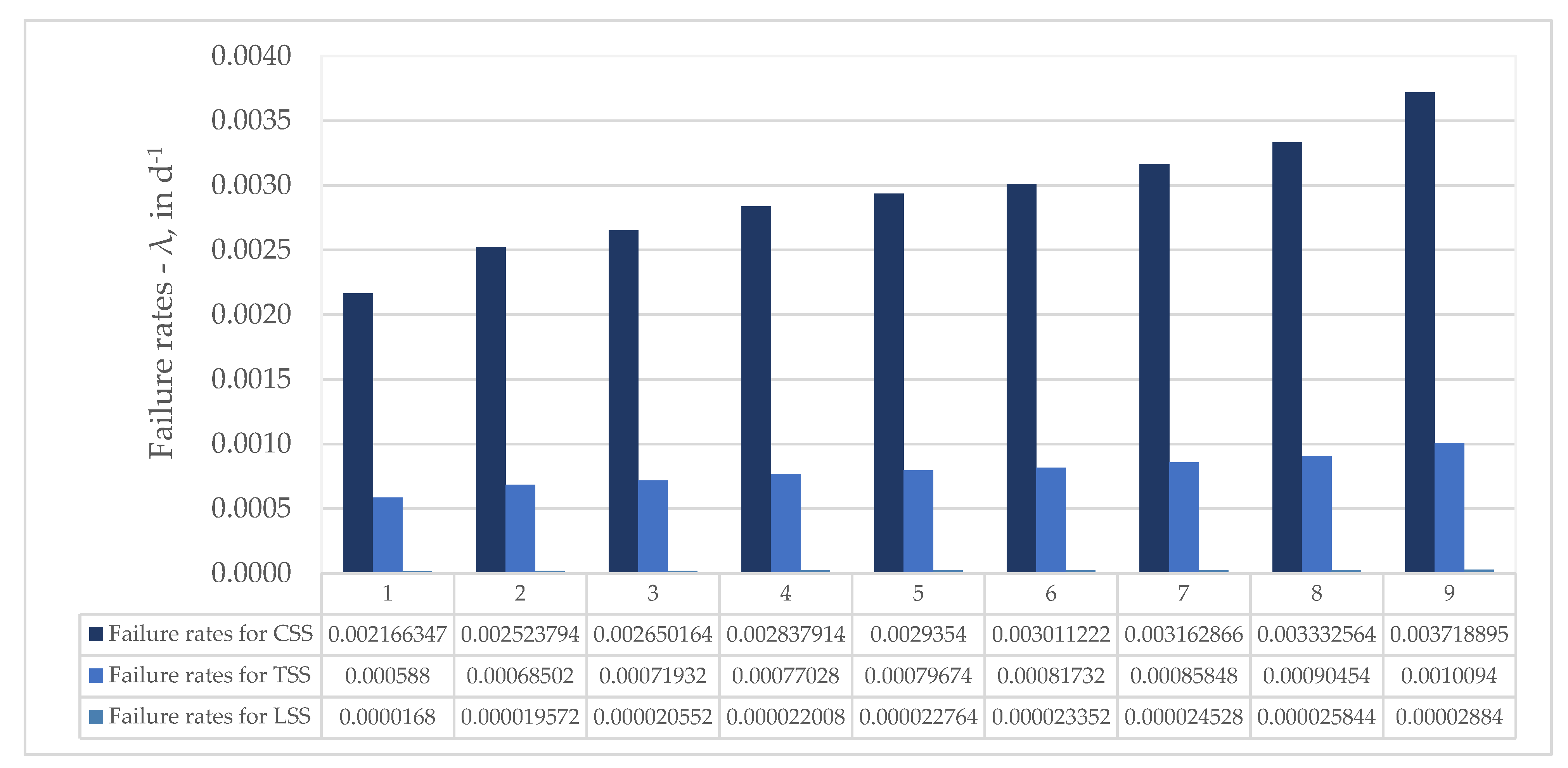
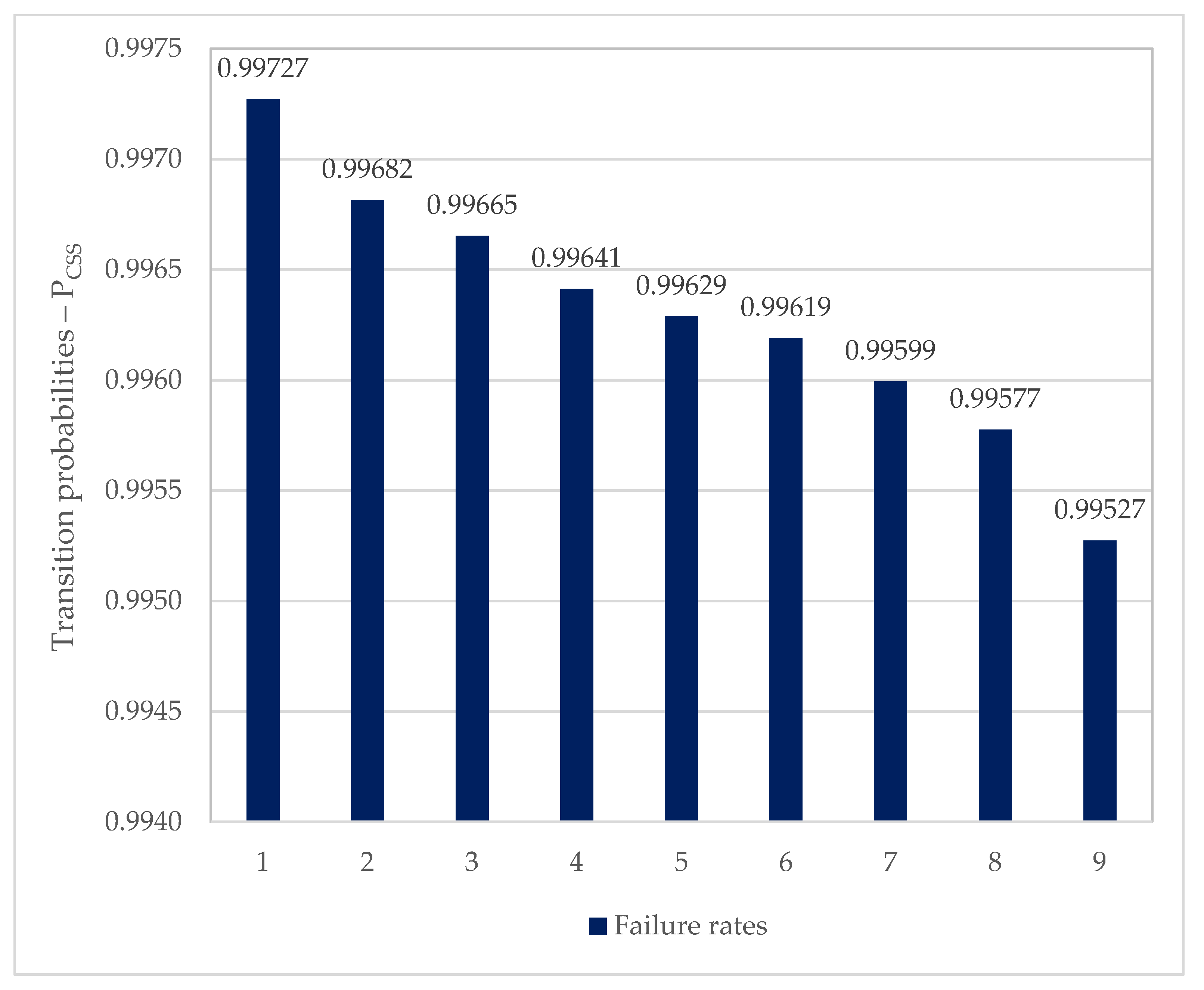
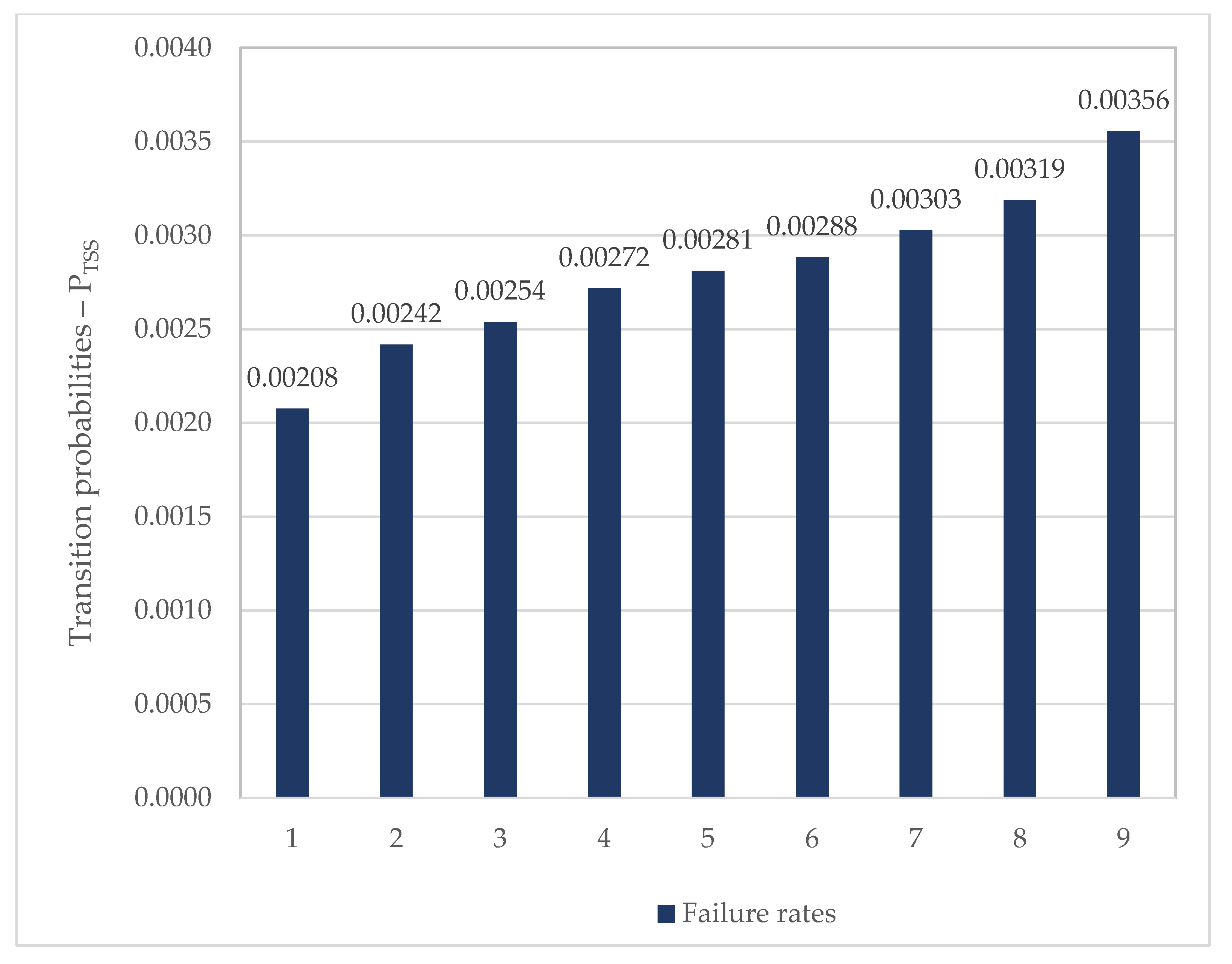
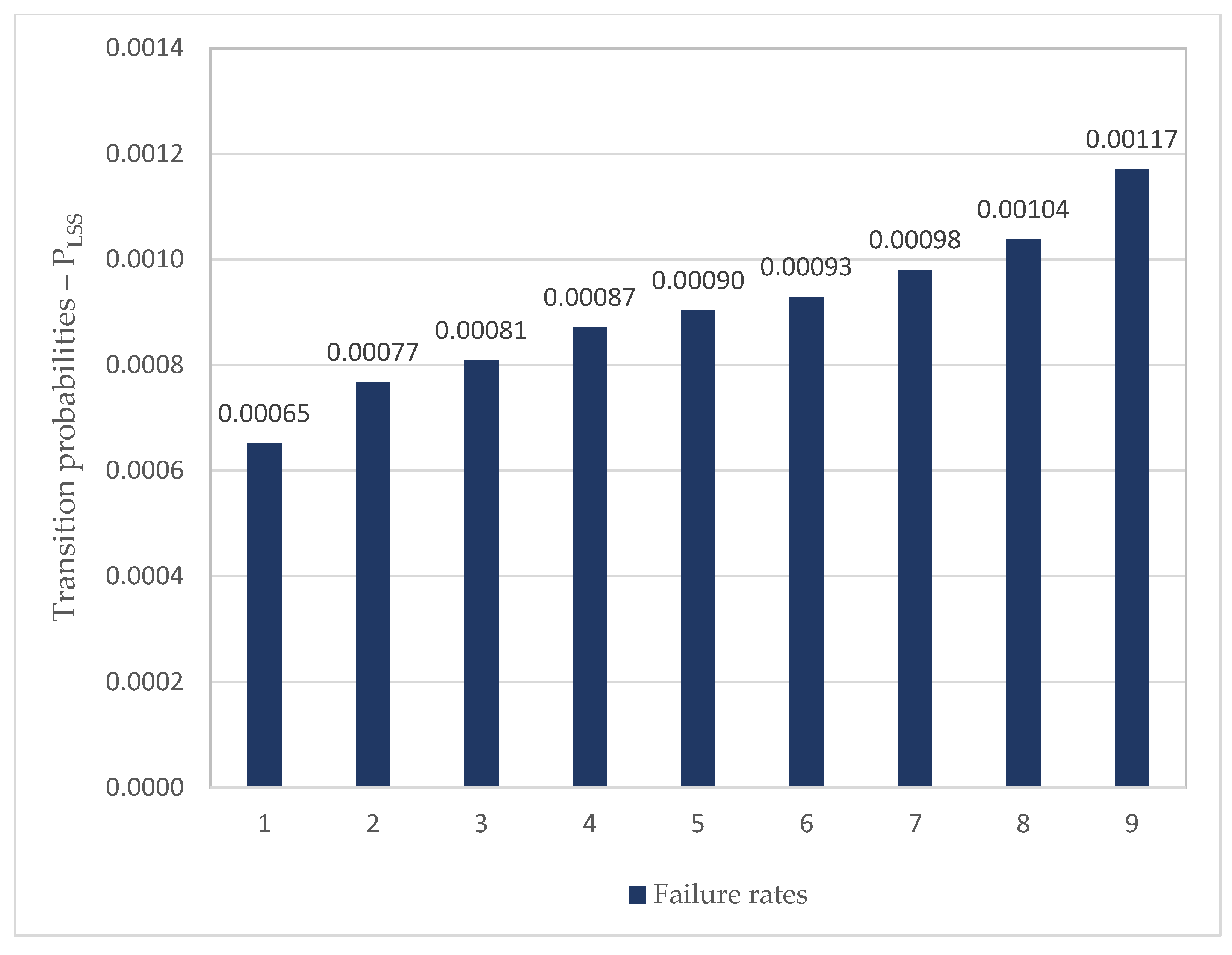
An exemplary analysis was performed using data from the literature and operating data from different WSSs to estimate the values of λ and constant μ. In Figure 2, Figure 3, Figure 4 and Figure 5, the failure rates for λCSS, λTSS, and λLSS, as well as the dependence of the PCSS, PTSS, and PLSS values on the failure rates λCSS, λTSS, and λLSS, for constant μTSS = 1.0399 d−1 and μLSS = 0.0276 d−1 are presented.
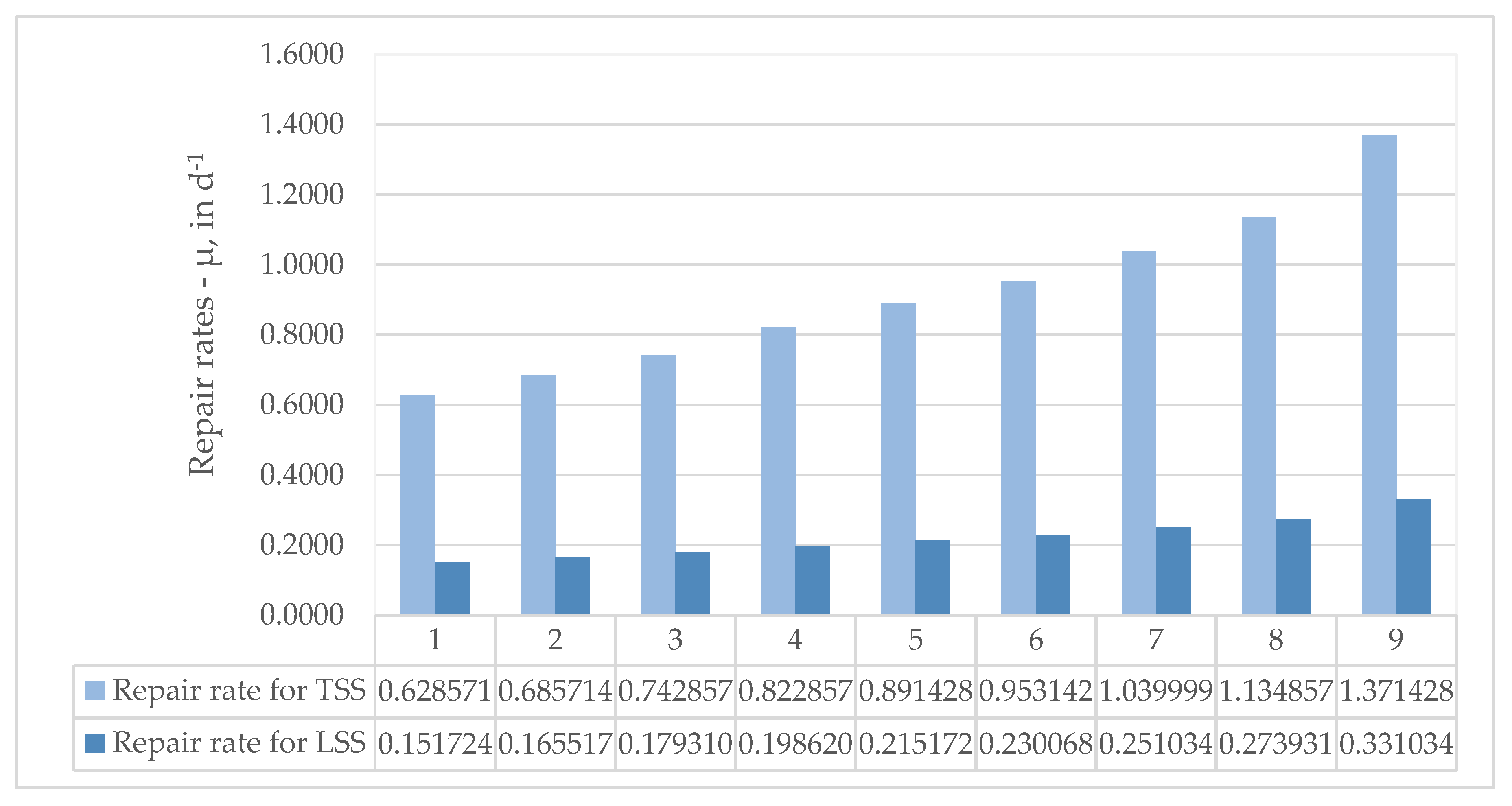
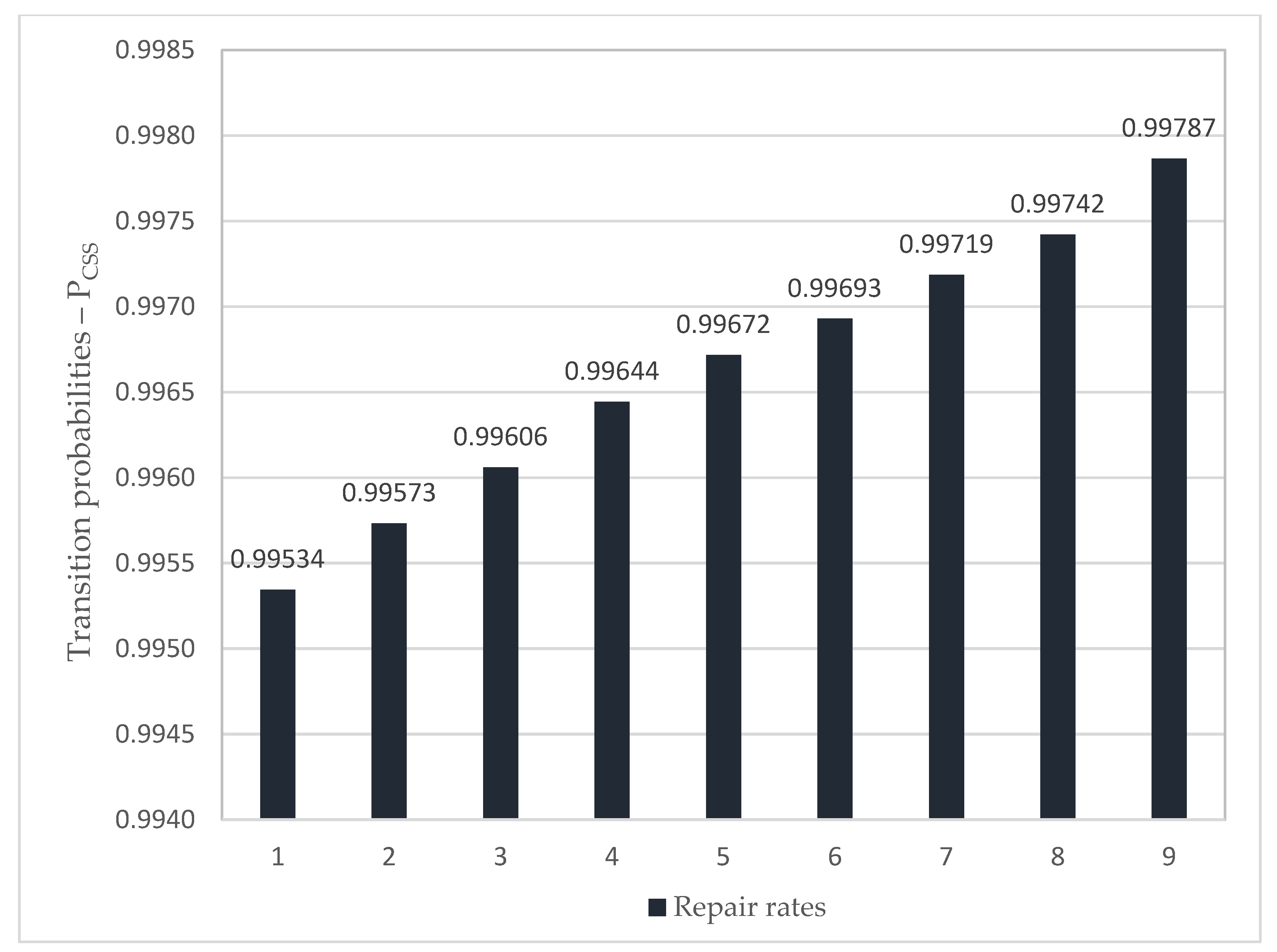
In Figure 6, Figure 7, Figure 8 and Figure 9, the repair rates for μTSS and μLSS, as well as the dependence of the values of PCSS, PTSS, and PLSS values on the repair rates for μTSS and μLSS, for constant failure rates λCSS = 0.0028379 d−1, λTSS = 0.0007703 d−1, and λLSS = 0.0000220 d−1 are presented.
The results were considerably dependent on the failure rate and rate of the repair. Since each defined state was characterized by a specific number of losses, determining each state means determining the probability that a threat to the system could occur.
5.2. The Case Study Results
The following assumptions were made for CSS, TSS, and LSS, based on many years of research on the water supply system:
- The occurrence of each of the three states is a random event that occurs with probabilities: PCSS(t), PTSS(t), PLSS(t);
- The WSS may be in one of the three distinguished states at any given time;
- There may be a transition from one state to another;
- At time t = 0, the subsystem is in the CSS state;
- Transition times between individual states have exponential distributions in accordance with the carried out statistical analysis through chi-square test;
- The failure rate and repair rate parameters are, respectively, λCSS, λTSS, λLSS, μCSS, μTSS, μLSS;
- The stream of damage is the simplest, i.e., a stationary Poisson stream.
The operational data used in the analysis concerned the failure rate of the examined water supply system and interruptions to the water supply. After a detailed analysis of the examined water supply system, the following values of mean time to repair (MTTR), calculated as the average time needed to determine the cause of (Mean Waiting Time to Repair—MWTTR), and repair fails (Mean Time to Repair—MTR) for each state were obtained:
- MTTR for TSS state: 0.875 days;
- MTTR for LSS state: 3.625 days.
And for the mean time between failures:
- MTBF for CSS state: 42.52 days (0.11 year);
- MTBF for TSS state: 1020.41 days (2.79 years);
- MTBF for LSS state: 35,714.29 days (97.85 years).
On the basis of the estimated times of MTTR and MTBF, the failure and repair rate parameters were determined.
5.3. Discussion
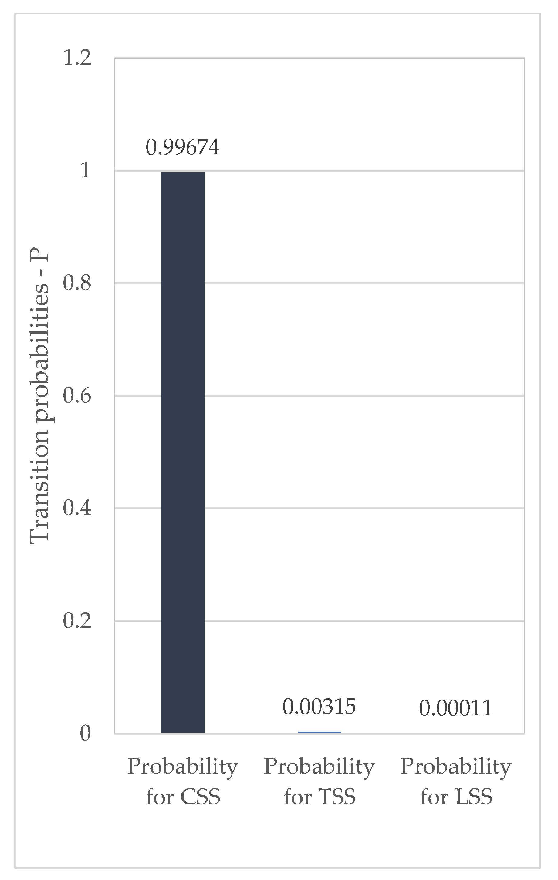
Taking into account the transition probabilities, based on the results of the analysis, it was determined that the PTSS of a partial WSS fault in the examined city regarding the lack of water supply to consumers was very low, indicating that the controlled state existed when the supply of water was interrupted or the water was of poor quality. The state of complete fault described by the probability PLSS was very low. This unacceptable state refers to a situation in which there is a real threat due to a break in water supply or bad quality water being consumed. In this regard, the PCSS of the tolerable state in the analyzed city was very high, which means the occurrence of incidental events in WSS was at low occurrence frequency, so the threat of water shortage or consumption of bad quality water was unexposed under favorable circumstances [23,39]. In addition, establishing the criteria values for states is an important issue, which should be achieved by collaborating teams of experts in safety assessment methods and experienced engineers, using the most current scientific and technological knowledge and data from the operating WSS [19]. The developed models require an extensive knowledge base of the intensity of transitions between states and knowledge of the distributions of individual probabilities. When this knowledge base does not meet the requirements in terms of the number of operating data, or simply lack of them, then expert knowledge can be used and fuzzy modeling can be applied [39]. The use of Markov models was applicable in the analysis conducted in terms of the occurrence of incidental events, resulting in disruptions in the functioning of the entire system, in comparison to the research performed on the basis of certain values of parameters in water distribution subsystems [44,45,46]. The developed models took into account the possibility of partial and complete system failure. The probability of the occurrence of a given state depends on the adopted model, which characterizes the given system through the network, hydraulic system, monitoring system, multibarrier system, etc. This allows using the model for any system of any specificity, which is essential in the context of the practical application of the proposed models.
6. Conclusions
Markov models for WSSs operations can be used to develop a computer simulation method that can predict the probability of failure for different types of WSSs. One of the most challenging aspects of WSSs is the ability to predict events that can lead to a loss of safety. All scenarios, even the most unlikely ones, are possible. There is only a limited amount that can be done to minimize the consequences and losses. It is possible to determine the values of the nonstationary probabilities at any time using the calculated values. This study presented operating models that can be modified for different, real operating systems.
As a result of the proposed approach for the water supply system, emergency conditions can be limited. Analysis of the failure rates of water supply systems, and, in particular, its modeling (i.e., mechanism of formation), through optimization of working and repair times, will reduce losses in the water supply system, which is crucial to reduce and optimize energy consumption. Research of this type should be the basis for sustainable water management to reduce the use of water resources and protect water ecosystems, which is part of the European Green Deal strategy.
The calculated values relative to the system safety indicated that the following category applies: tolerable state, which means that the WSS performs its functions in a safe and reliable manner. The controlled state requires improvement in the performance of certain elements of the system (e.g., network monitoring, protective stations), and the repair of certain sections of the water distribution network should be considered. An unacceptable state signifies that the WSS does not meet its intended functions, both in terms of operational reliability and safety. An analysis of the main factors is required, and the WSS should be completely redesigned or modernized.
Water supply system strategies should take into account the following factors: the risk of disruption to the water supply; the possibility of biological or chemical pollution at the source and within the water distribution system; the risk of biological or mineral contamination; the risk of malevolent actions; as well as the cost of corrective actions to provide water from alternative sources to consumers.
It is important to assess the threats associated with crisis management regarding critical infrastructure, including drinking water systems, on a case-by-case basis. There is always a problem of providing drinking water to the population in a variety of crisis situations, such as floods, droughts, earthquakes, breakdowns, technical disasters, blackouts, etc.
Diseases and epidemics occur as a result of a lack of these supplies. It is also important to note that the WSS itself can result in a crisis if various adverse events occur, resulting in the unreliable functioning of the system and consequently, a loss of consumer safety. To develop a comprehensive safety management program for the drinking water supply system, it is imperative that emergency drinking water supply plans are developed for a variety of crisis situations, as well as a detailed risk analysis of the possibility of adverse events occurring in the system.
The method of analyzing and assessing the operational safety of the water supply system proposed in this paper forms the basis for the risk management process and for making modernization and renovation decisions of water supply companies.
The major issue is the optimization of the operation of the critical infrastructures: connected water and energy systems. It is a multicriteria optimization issue as it covers the minimization of water losses, and therefore, the energy used in water supply systems, the maximization of operational reliability and safety, and the minimization of sanitary risks. The issue becomes even more significant if one considers the transition to sustainable energy in accordance with EU standards and recommendations that should be implemented: good engineering practices; design; construction; and operation phases of the system. The proposed assessment can also be applied in energy supply systems, given the relative universality of the approach presented here.
Author Contributions
All authors equally contributed to the development of this manuscript. All authors have read and agreed to the published version of the manuscript.
Funding
This research received no external funding.
Data Availability Statement
Not applicable.
Conflicts of Interest
The authors declare no conflict of interest.
References
- United Nations. Transforming Our World: The 2030 Agenda for Sustainable Development, 21 October 2015. Available online: https://sdgs.un.org/sites/default/files/publications/21252030%20Agenda%20for%20Sustainable%20Development%20web.pdf (accessed on 1 January 2023).
- Chiqueta, J.; Limniosa, N.; Eid, M. Piecewise deterministic Markov processes applied to fatigue crack growth modelling. J. Stat. Plan. Inference 2009, 139, 1657–1667. [Google Scholar] [CrossRef]
- United Nations. Resolution Adopted by the General Assembly on 28 July 2010 (A/64/L.63/Rev.1 and Add.1) 64/292. The Human Right to Water and Sanitation, 2010. Available online: https://unece.org/fileadmin/DAM/env/water/publications/WH_17_Human_Rights/ECE_MP.WH_17_ENG.pdf (accessed on 1 January 2023).
- Resolution No 1693/2009 of the parliamentary Assembly of the Council of Europe, 2 October 2009. Available online: https://assembly.coe.int/nw/xml/XRef/Xref-XML2HTML-en.asp?fileid=17786&lang=en (accessed on 1 January 2023).
- Directive (EU) 2020/2184 of the European Parliament and of the Council of 16 December 2020 on the Quality of Water Intended for Human Consumption, OJ L 435, 23 December 2020. Available online: https://eur-lex.europa.eu/legal-content/EN/TXT/PDF/?uri=CELEX:32020L2184&from=EN (accessed on 20 December 2020).
- World Health Organization. Guidelines for Drinking-Water Quality, 4th ed.; World Health Organization: Geneva, Switzerland, 2011; Available online: https://apps.who.int/iris/bitstream/handle/10665/44584/9789241548151_eng.pdf;jsessionid=FB26DE4E81767BC7525DC61A1537C754?sequence=1 (accessed on 15 December 2022).
- Kordana-Obuch, S.; Starzec, M.; Słyś, D. Assessment of the Feasibility of Implementing Shower Heat Exchangers in Residential Buildings Based on Users’ Energy Saving Preferences. Energies 2021, 14, 5547. [Google Scholar] [CrossRef]
- Rak, J.R.; Wartalska, K.; Kaźmierczak, B. Weather Risk Assessment for Collective Water Supply and Sewerage Systems. Water 2021, 13, 1970. [Google Scholar] [CrossRef]
- Żywiec, J.; Szpak, D.; Piegdoń, I.; Boryczko, K.; Pietrucha-Urbanik, K.; Tchórzewska-Cieślak, B.; Rak, J. An Approach to Assess the Water Resources Reliability and Its Management. Resources 2023, 12, 4. [Google Scholar] [CrossRef]
- Ma, Q.; Zhang, J.; Xiong, B.; Zhang, Y.; Ji, C.; Zhou, T. Quantifying the Risks that Propagate from the Inflow Forecast Uncertainty to the Reservoir Operations with Coupled Flood and Electricity Curtailment Risks. Water 2021, 13, 173. [Google Scholar] [CrossRef]
- Rak, J.R.; Tchórzewska-Cieślak, B.; Pietrucha-Urbanik, K. A Hazard Assessment Method for Waterworks Systems Operating in Self-Government Units. Int. J. Environ. Res. Public Health 2019, 16, 767. [Google Scholar] [CrossRef] [Green Version]
- Morosini, A.F.; Haghshenas, S.S.; Shaffiee Haghshenas, S.; Choi, D.Y.; Geem, Z.W. Sensitivity Analysis for Performance Evaluation of a Real Water Distribution System by a Pressure Driven Analysis Approach and Artificial Intelligence Method. Water 2021, 13, 1116. [Google Scholar] [CrossRef]
- Zeleňáková, M.; Markovič, G.; Kaposztásová, D.; Vranayová, Z. Rainwater management in compliance with sustainable design of buildings. Procedia Eng. 2014, 89, 1515–1521. [Google Scholar] [CrossRef] [Green Version]
- Dettori, M.; Azara, A.; Loria, E.; Piana, A.; Masia, M.D.; Palmieri, A.; Cossu, A.; Castiglia, P. Population Distrust of Drinking Water Safety. Community Outrage Analysis, Prediction and Management. Int. J. Environ. Res. Public Health 2019, 16, 1004. [Google Scholar] [CrossRef] [Green Version]
- Zielina, M.; Dąbrowski, W. Energy and Water Savings during Backwashing of Rapid Filter Plants. Energies 2021, 14, 3782. [Google Scholar] [CrossRef]
- Wu, C.; Wang, X.; Jin, J.; Zhou, Y.; Bai, X.; Zhou, L.; Tong, F.; Zhang, L.; Cui, Y. Structure Simulation and Equilibrium Evaluation Analysis of Regional Water Resources, Society, Economy and Ecological Environment Complex System. Entropy 2023, 25, 181. [Google Scholar] [CrossRef] [PubMed]
- Zhang, W.; Lai, T.; Li, Y. Risk Assessment of Water Supply Network Operation Based on ANP-Fuzzy Comprehensive Evaluation Method. J. Pipeline Syst. Eng. Pract. 2022, 13, 04021068. [Google Scholar] [CrossRef]
- Chybowski, L. Importance Analysis of Components of a Multi-Operational-State Power System Using Fault Tree Models. Information 2020, 11, 29. [Google Scholar] [CrossRef] [Green Version]
- Tchórzewska-Cieślak, B. Urban Water Safety Management. Chem. Eng. Trans. 2012, 26, 201–206. [Google Scholar] [CrossRef]
- Yang, Z.; Barroca, B.; Weppe, A.; Bony-Dandrieux, A.; Laffréchine, K.; Daclin, N.; November, V.; Omrane, K.; Kamissoko, D.; Benaben, F.; et al. Indicator-based resilience assessment for critical infrastructures—A review. Saf. Sci. 2023, 160, 106049. [Google Scholar] [CrossRef]
- Barton, N.A.; Farewell, T.S.; Hallett, S.H.; Acland, T.F. Improving pipe failure predictions: Factors affecting pipe failure in drinking water networks. Water Res. 2019, 164, 114926. [Google Scholar] [CrossRef]
- Stark, M.R. Mathematical Foundations for Design; McGraw-Hill Book Company: New York, NY, USA, 1972. [Google Scholar]
- Tchórzewska-Cieślak, B.; Rak, J. Models of safety reliability of water supply systems using Markov processes. In II National Congress of Environmental Engineering; Committee of Environmental Engineering of the Polish Academy of Sciences: Lublin, Poland, 2005; Volume 32, pp. 519–528. [Google Scholar]
- Lee, M.-H.; Chen, Y.J. Precipitation Modeling for Extreme Weather Based on Sparse Hybrid Machine Learning and Markov Chain Random Field in a Multi-Scale Subspace. Water 2021, 13, 1241. [Google Scholar] [CrossRef]
- Rafiq, M.; Akbar, A.; Maqbool, S.; Sokolová, M.; Haider, S.A.; Naz, S.; Danish, S.M. Corporate Risk Tolerance and Acceptability towards Sustainable Energy Transition. Energies 2022, 15, 459. [Google Scholar] [CrossRef]
- Richter, K.; Santos, D.C.d.; Schmid, A.L. Efficiency Analysis of Water Conservation Measures in Sanitary Infrastructure Systems by Means of a Systemic Approach. Sustainability 2020, 12, 3055. [Google Scholar] [CrossRef] [Green Version]
- Cox, D.R.; Miller, H.D. The Theory of Stochastic Processes; Chapman& Hall/CRC: Boca Raton, FL, USA, 1996; Available online: https://scholar.google.com/scholar_lookup?title=The+Theory+of+Stochastic+Processes&author=Cox,+D.R.&author=Miller,+H.D.&publication_year=1996 (accessed on 1 January 2023).
- Grabski, F. Reliability and maintainability characteristics in semi-Markov model. J. Pol. Saf. Reliab. Assoc. 2016, 7, 79–85. [Google Scholar]
- Grabski, F. Stochastic Systems Availabity Models. In Materials of the XXXVI Winter School of Reliability; Warsaw University of Technology, Polish Academy of Sciences: Warsaw, Poland, 2008; pp. 112–128. [Google Scholar]
- Papciak, D.; Domoń, A.; Zdeb, M.; Skwarczyńska-Wojsa, A.; Konkol, J. Optimization of Quantitative Analysis of Biofilm Cell from Pipe Materials. Coatings 2021, 11, 1286. [Google Scholar] [CrossRef]
- Tchórzewska-Cieślak, B.; Pietrucha-Urbanik, K.; Kuliczkowska, E. An Approach to Analysing Water Consumers’ Acceptance of Risk-Reduction Costs. Resources 2020, 9, 132. [Google Scholar] [CrossRef]
- Valis, D.; Forbelská, M.; Vintr, Z. Forecasting study of mains reliability based on sparse field data and perspective models. Maint. Reliab. 2020, 22, 179–191. [Google Scholar] [CrossRef]
- AL-Washali, T.; Sharma, S.; AL-Nozaily, F.; Haidera, M.; Kennedy, M. Modelling the Leakage Rate and Reduction Using Minimum Night Flow Analysis in an Intermittent Supply System. Water 2019, 11, 48. [Google Scholar] [CrossRef] [Green Version]
- Klimczak, T.; Paś, J.; Duer, S.; Rosiński, A.; Wetoszka, P.; Białek, K.; Mazur, M. Selected Issues Associated with the Operational and Power Supply Reliability of Fire Alarm Systems. Energies 2022, 15, 8409. [Google Scholar] [CrossRef]
- Młyński, D.; Bergel, T.; Młyńska, A.; Kudlik, K. A study of the water supply system failure in terms of the seasonality: Analysis by statistical approaches. AQUA Water Infrastruct. Ecosyst. Soc. 2021, 70, 289–302. [Google Scholar] [CrossRef]
- Tchórzewska-Cieślak, B. Methods for Analyzing and Assessing the Risk of Failure of the Water Distribution Subsystem; Rzeszów University of Technology Publishing House: Rzeszow, Poland, 2011. [Google Scholar]
- Tchorzewska-Cieslak, B.; Rak, J. Method of Identification of Operational States of Water Supply System; Environmental Engineering; Taylor & Francis: London, UK, 2009; Volume 3, pp. 521–526. [Google Scholar]
- Jaźwiński, J.; Ważyńska-Fiok, K. Systems Safety; PWN: Warsaw, Poland, 1993. [Google Scholar]
- Tchórzewska-Cieślak, B. The Multifaceted Analysis of Safety in the Operation of Water Supply Systems; Publishing House of the Rzeszow University of Technology: Rzeszow, Poland, 2018; Available online: https://eksiegarnia.pl/wieloaspektowa-analiza-bezpieczenstwa-w-eksploatac,3,187,97299 (accessed on 1 December 2022).
- Kolowrocki, K.; Soszynska-Budny, J. Modeling Complex Technical Systems Operation Processes. Reliab. Saf. Complex Tech. Syst. Process. 2011, 53–78. [Google Scholar] [CrossRef]
- Davis, M.H.A. Markov Models and Optimization; Monographs on Statistics and Applied Probability 49; Chapman& Hall/CRC: Boca Raton, FL, USA, 1993. [Google Scholar]
- EN 15975-2:2013. Safety of Drinking Water Supply. Guidelines for Risk and Crisis Management. Risk Management. Available online: https://standards.iteh.ai/catalog/standards/sist/dd2df50c-59ec-40f4-845a-00b83dfdd6df/sist-en-15975-2-2013 (accessed on 9 December 2022).
- Rak, J. Safety of Water Supply System; Polish Academy of Science: Warsaw, Poland, 2009. [Google Scholar]
- Pietrucha-Urbanik, K.; Tchórzewska-Cieślak, B.; Eid, M. A Case Study in View of Developing Predictive Models for Water Supply System Management. Energies 2021, 14, 3305. [Google Scholar] [CrossRef]
- Pietrucha-Urbanik, K.; Tchórzewska-Cieślak, B.; Eid, M. Water Network-Failure Data Assessment. Energies 2020, 13, 2990. [Google Scholar] [CrossRef]
- Tchórzewska-Cieślak, B.; Pietrucha-Urbanik, K.; Eid, M. Functional Safety Concept to Support Hazard Assessment and Risk Management in Water-Supply Systems. Energies 2021, 14, 947. [Google Scholar] [CrossRef]
Figure 1.
Variants of the possibilities of transitions between the safety states of the WSS (based on the work of [23,37,39]), where CSS is a complete safety state, TSS is a threat to the safety state, and LSS is a loss of safety state. λ is the failure rate and µ is the repair rate, respectively, for each state.


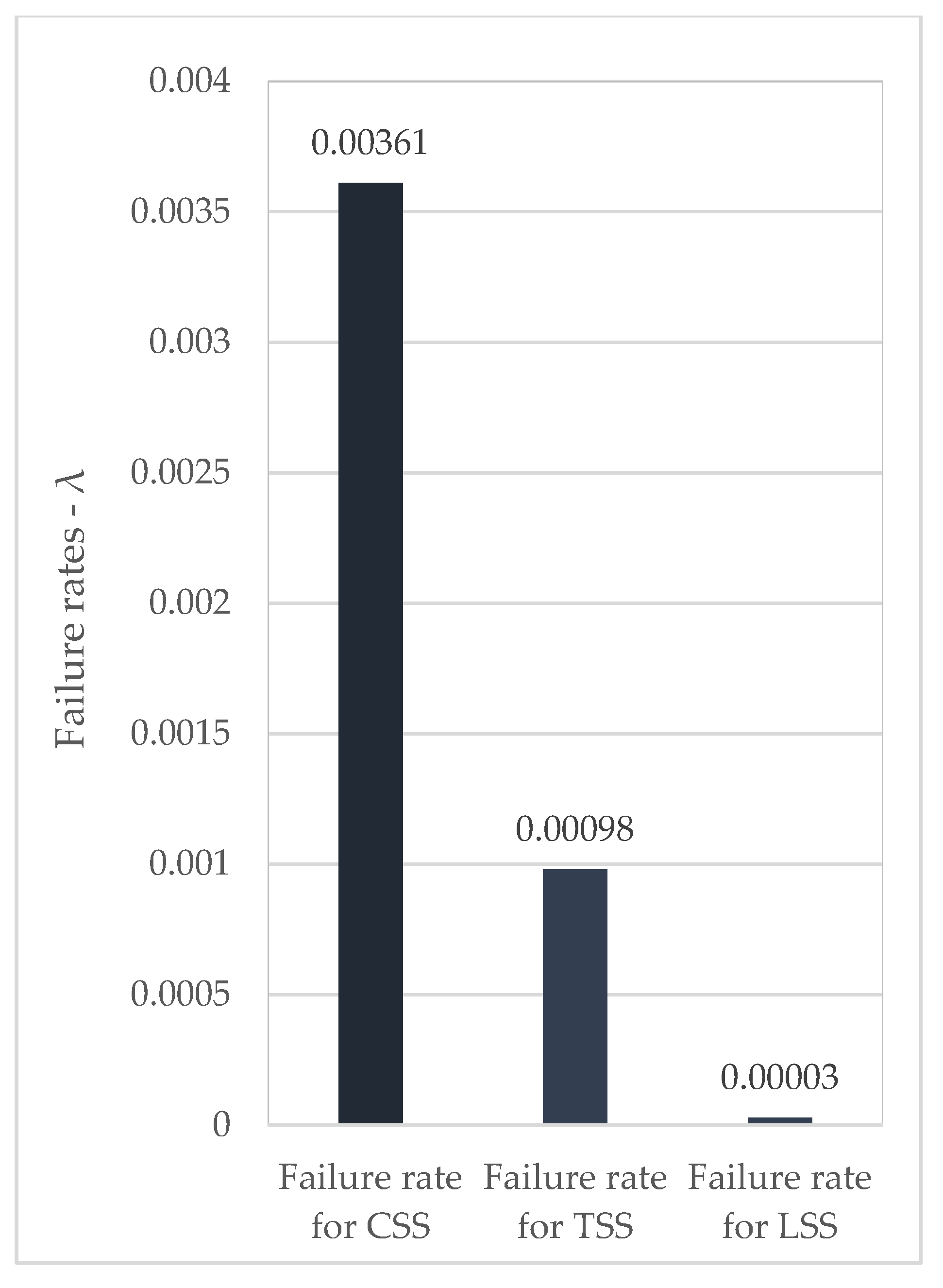
Figure 2.
Failure rates for λCSS, λTSS, and λLSS.

Figure 3.
Dependence of the PCSS values on the failure rates λCSS, λTSS, and λLSS acc. to Figure 2, for the constant μTSS = 1.0399 d−1 and μLSS = 0.0276 d−1.
Figure 3.
Dependence of the PCSS values on the failure rates λCSS, λTSS, and λLSS acc. to Figure 2, for the constant μTSS = 1.0399 d−1 and μLSS = 0.0276 d−1.

Figure 4.
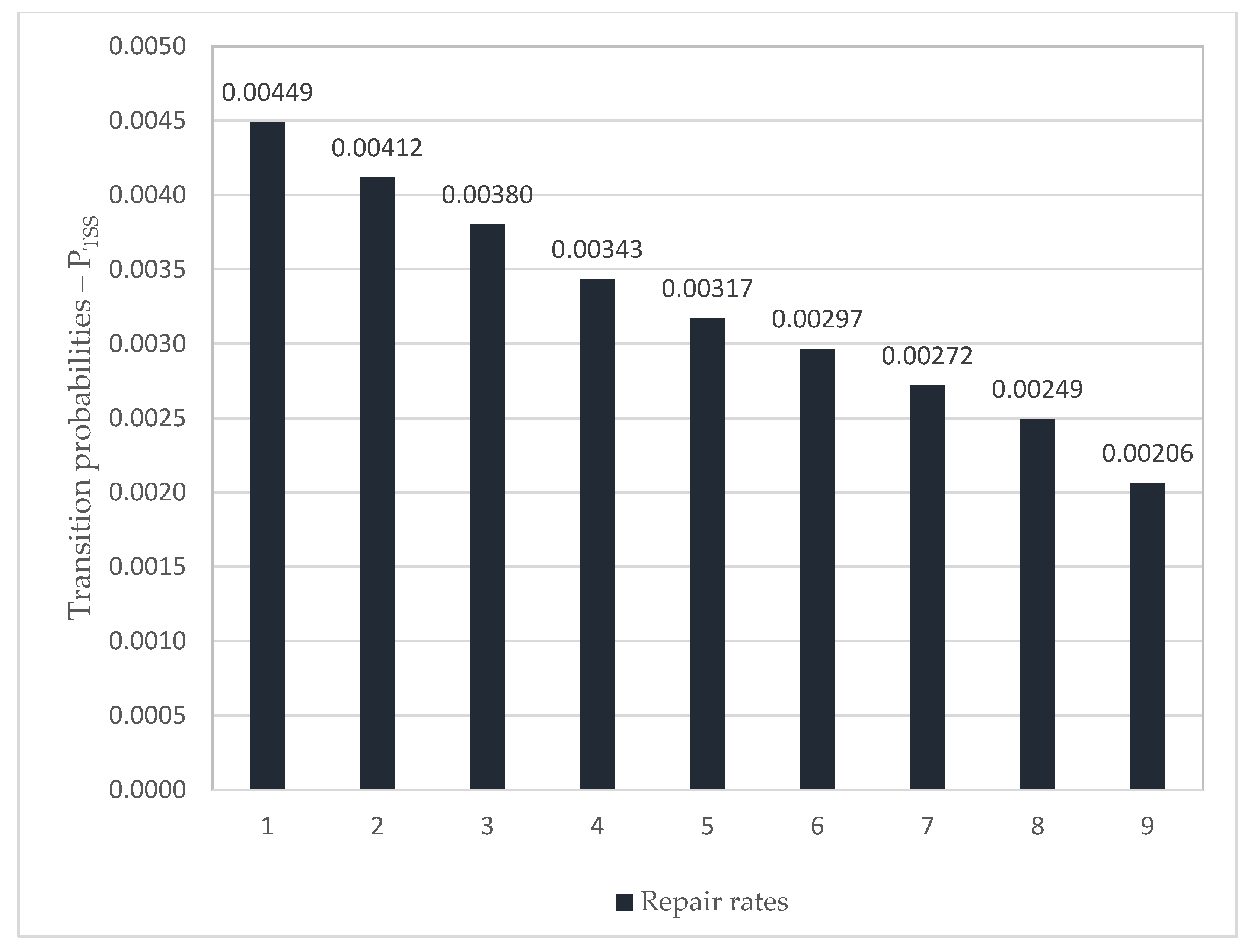
Dependence of the PTSS values on the failure rates λCSS, λTSS, and λLSS acc. to Figure 2, for the constant μTSS = 1.0399 d−1 and μLSS = 0.0276 d−1.
Figure 4.
Dependence of the PTSS values on the failure rates λCSS, λTSS, and λLSS acc. to Figure 2, for the constant μTSS = 1.0399 d−1 and μLSS = 0.0276 d−1.

Figure 5.
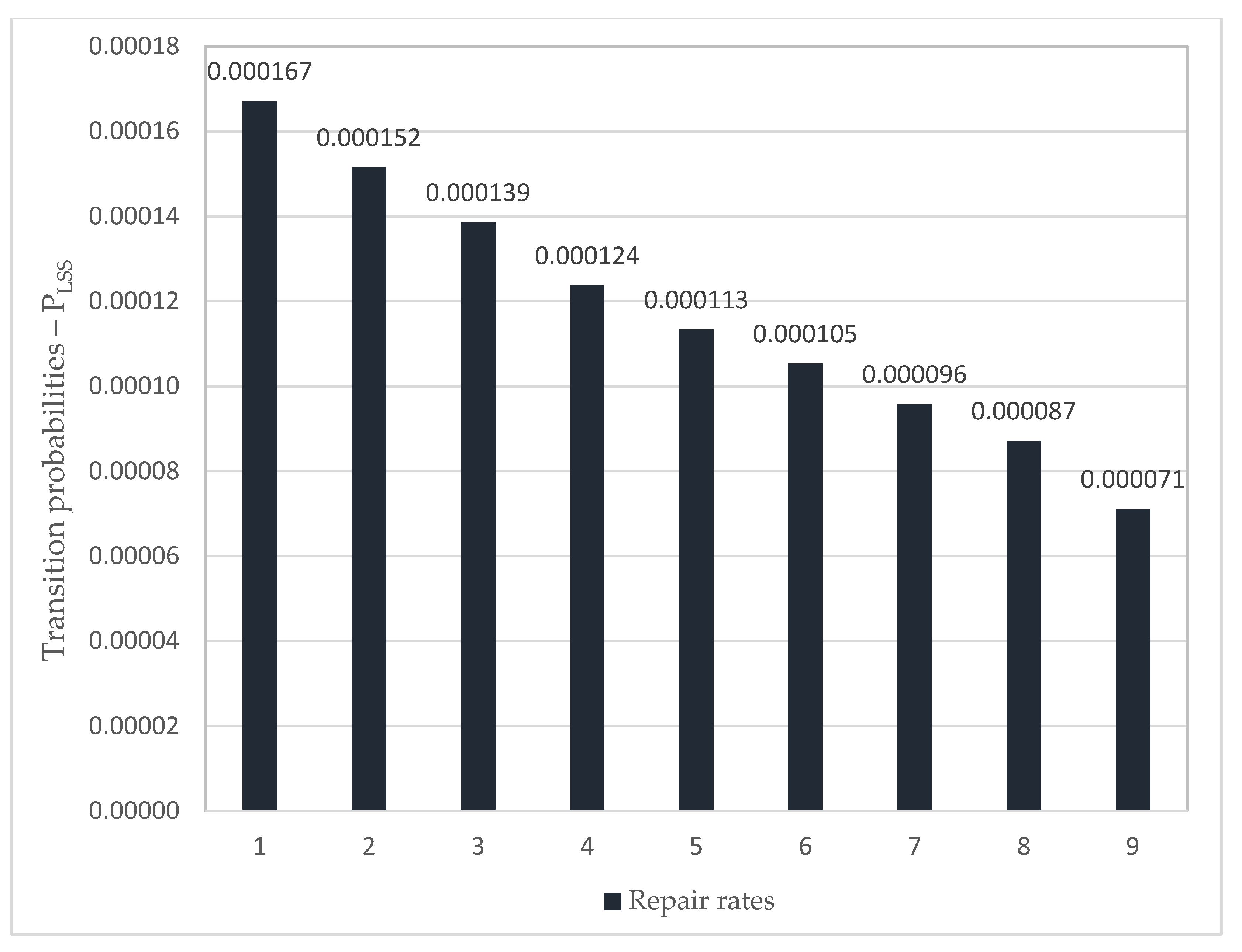
Dependence of the PLSS values on the failure rates λCSS, λTSS, and λLSS acc. to Figure 2, for the constant μTSS = 1.0399 d−1 and μLSS = 0.0276 d−1.
Figure 5.
Dependence of the PLSS values on the failure rates λCSS, λTSS, and λLSS acc. to Figure 2, for the constant μTSS = 1.0399 d−1 and μLSS = 0.0276 d−1.

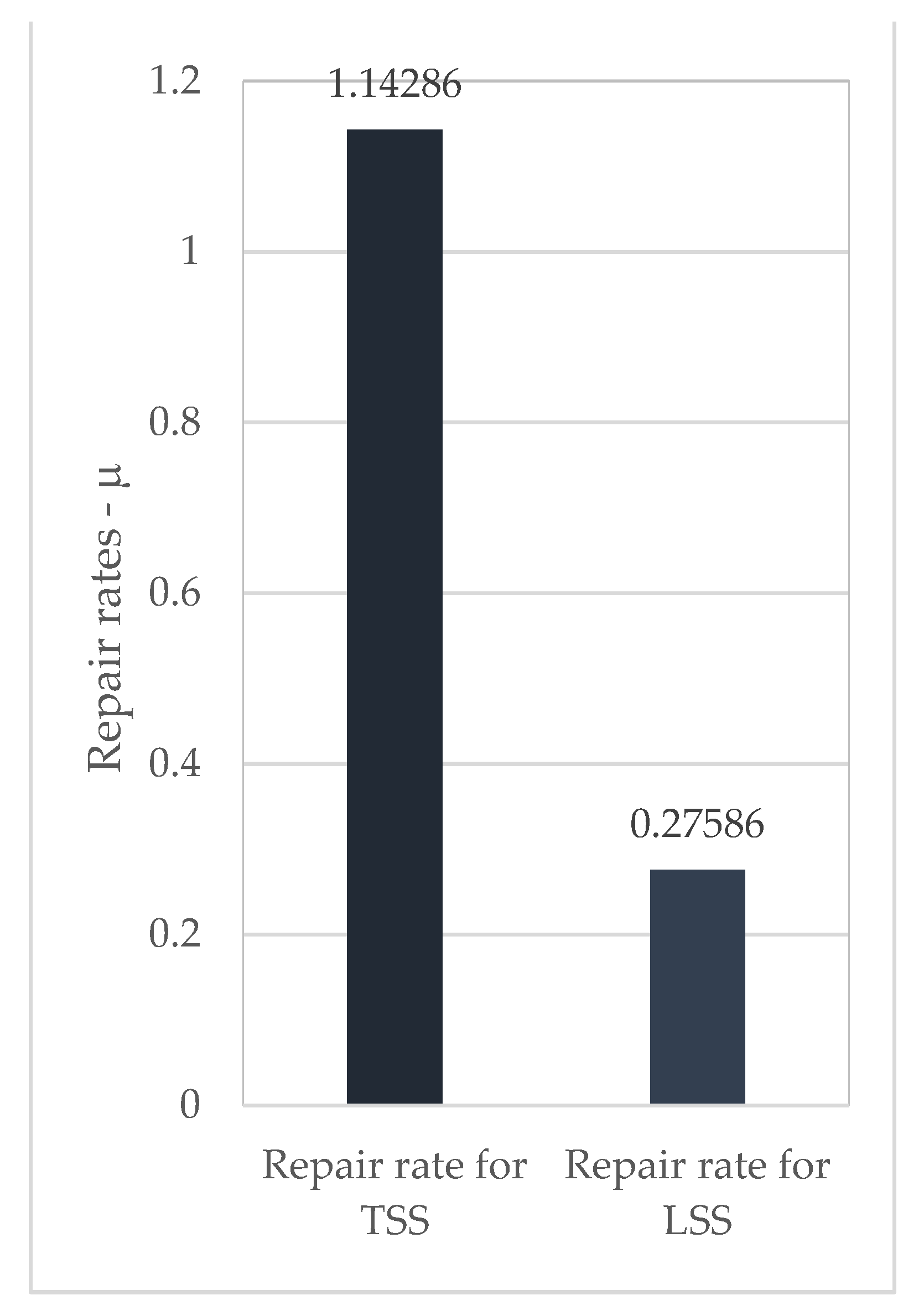
Figure 6.
Repair rates for μTSS and μLSS.

Figure 7.
Dependence of the PCSS values on the repair rates μTSS and μLSS acc. to Figure 6, for constant failure rates λCSS = 0.0028379 d−1, λTSS = 0.0007703 d−1, and λLSS = 0.0000220 d−1.
Figure 7.
Dependence of the PCSS values on the repair rates μTSS and μLSS acc. to Figure 6, for constant failure rates λCSS = 0.0028379 d−1, λTSS = 0.0007703 d−1, and λLSS = 0.0000220 d−1.

Figure 8.
Dependence of the PTSS values on the repair rates μTSS and μLSS acc. to Figure 6, for constant failure rates λCSS = 0.0028379 d−1, λTSS = 0.0007703 d−1, and λLSS = 0.0000220 d−1.
Figure 8.
Dependence of the PTSS values on the repair rates μTSS and μLSS acc. to Figure 6, for constant failure rates λCSS = 0.0028379 d−1, λTSS = 0.0007703 d−1, and λLSS = 0.0000220 d−1.

Figure 9.
Dependence of the PLSS values on the repair rates μTSS and μLSS acc. to Figure 6, for constant failure rates: λCSS = 0.0028379 d−1, λTSS = 0.0007703 d−1, and λLSS = 0.0000220 d−1.
Figure 9.
Dependence of the PLSS values on the repair rates μTSS and μLSS acc. to Figure 6, for constant failure rates: λCSS = 0.0028379 d−1, λTSS = 0.0007703 d−1, and λLSS = 0.0000220 d−1.

Figure 10.
Failure rates—λCSS, λTSS, and λLSS.

Figure 11.
Repair rates—μTSS and μLSS.

Figure 12.
Transition probabilities corresponding to individual states—PCSS, PTSS, and PLSS.

Disclaimer/Publisher’s Note: The statements, opinions and data contained in all publications are solely those of the individual author(s) and contributor(s) and not of MDPI and/or the editor(s). MDPI and/or the editor(s) disclaim responsibility for any injury to people or property resulting from any ideas, methods, instructions or products referred to in the content. |
© 2023 by the authors. Licensee MDPI, Basel, Switzerland. This article is an open access article distributed under the terms and conditions of the Creative Commons Attribution (CC BY) license (https://creativecommons.org/licenses/by/4.0/).
Share and Cite
MDPI and ACS Style
Tchórzewska-Cieślak, B.; Pietrucha-Urbanik, K. Water System Safety Analysis Model. Energies 2023, 16, 2809. https://0-doi-org.brum.beds.ac.uk/10.3390/en16062809
AMA Style
Tchórzewska-Cieślak B, Pietrucha-Urbanik K. Water System Safety Analysis Model. Energies. 2023; 16(6):2809. https://0-doi-org.brum.beds.ac.uk/10.3390/en16062809
Chicago/Turabian StyleTchórzewska-Cieślak, Barbara, and Katarzyna Pietrucha-Urbanik. 2023. "Water System Safety Analysis Model" Energies 16, no. 6: 2809. https://0-doi-org.brum.beds.ac.uk/10.3390/en16062809
Note that from the first issue of 2016, this journal uses article numbers instead of page numbers. See further details here.