
Optimization of Fracturing Parameters by Modified Genetic Algorithm in Shale Gas Reservoir
Research Institute of Petroleum Exploration and Development, No. 20 Xueyuan Road, Haidian District, Beijing 100083, China
*
Author to whom correspondence should be addressed.
Energies 2023, 16(6), 2868; https://0-doi-org.brum.beds.ac.uk/10.3390/en16062868
Submission received: 15 February 2023
/
Revised: 15 March 2023
/
Accepted: 17 March 2023
/
Published: 20 March 2023
(This article belongs to the Special Issue Environmental Analysis, Monitoring, and Optimization of Unconventional Oil and Gas Extraction)
Abstract
:Shale gas reservoirs have extremely low porosity and permeability, making them challenging to exploit. The best method for increasing recovery in shale gas reservoirs is horizontal well fracturing technology. Hence, fracturing parameter optimization is necessary to enhance shale gas horizontal fracturing well production. Traditional optimization methods, however, cannot meet the requirements for overall optimization of fracturing parameters. As for intelligent optimization algorithms, most have excellent global search capability but incur high computation costs, which limits their usefulness in real-world engineering applications. Thus, a modified genetic algorithm combined based on the Spearman correlation coefficient (SGA) is proposed to achieve the rapid optimization of fracturing parameters. SGA determines the crossover and mutation rates by calculating the Spearman correlation coefficient instead of randomly determining the rates like GA does, so that it could quickly converge to the optimal solution. Within a particular optimization time, SGA could perform better than GA. In this study, a production prediction model is established by the XGBoost algorithm based on the dataset obtained by simulating the shale gas multistage fracturing horizontal well development. The result shows that the XGBoost model performs well in predicting shale gas fracturing horizontal well production. Based on the trained XGBoost model, GA, SGA, and SGD were used to optimize the fracturing parameters with the 30-day cumulative production as the optimization objective. This process has conducted nine fracturing parameter optimization tests under different porosity and permeability conditions. The results show that, compared with GA and SGD, SGA has faster speed and higher accuracy. This study’s findings can help optimize the fracturing parameters faster, resulting in improving the production of shale gas fracturing horizontal wells.
1. Introduction
Natural gas now accounts for an increasing proportion of energy due to the ongoing transition of the domestic energy system to clean energy [1,2,3]. However, the development of conventional gas to meet the demand of the energy market is difficult. Thus, it is necessary to increase the development of unconventional gas [4,5,6].
Shale gas is a kind of unconventional gas with significant reserves in the world [7]. However, compared with conventional reservoirs, shale gas reservoirs have super-low permeability and porosity [8]. Moreover, shale gas typically exists in shale through adsorption and free state [9]. Due to the characteristics of shale gas reservoirs, achieving unconventional gas economic recovery is challenging using conventional reservoir development methods. Shale gas reservoirs are mainly developed through horizontal well fracturing technology [10,11,12]. Hence, it is necessary to design reasonable fracturing parameters for horizontal well fracturing technology.
Fracturing parameter design is usually achieved thanks to optimization methods, which aim to obtain a combination of fracturing parameters with the maximum target parameters [13,14]. Generally, the target parameters are productivity indicators, such as production, net present value, and so on [15]. Therefore, productivity prediction of shale gas horizontal wells is critical for optimizing the fracturing parameters of shale gas horizontal wells. Usually, a fast and accurate productivity prediction model is necessary to decrease the optimization time and ensure optimization accuracy.
According to the calculating theory, productivity prediction models are classified into three categories: analytical models [16], numerical simulation models [17], and data-driven models [18]. Analytical and numerical simulation models are derived from the oil and gas seepage theory to obtain an analytical solution. The analytical model calculates fast but its prediction accuracy is limited to too many assumptions. Numerical simulation models have higher prediction accuracy than analytical models but are time-consuming and require plenty of complex reservoir data, such as fault, structure, sedimentary facies zone, and so on. Data-driven models, established by machine learning methods, can meet the requirements of calculation speed and accuracy for fracturing parameters optimization. Wang et al. [19] predicted shale gas production with a Multi-layer Perceptron (MLP) network and Long Short-term Memory (LSTM) network. Xue et al. [20] compared the performance of Multi-objective Random Forest (MORF) and Multi-output Regression Chain (MORC) in shale gas production prediction. However, every machine learning algorithm has its adaptability for different problems.
There are two kinds of fracturing optimization methods: traditional optimization [21,22,23] and intelligent optimization [24,25,26]. The traditional optimization method mainly optimizes the fracturing parameters one by one by sensitivity analysis. Jiang et al. [27] optimized the fracturing parameters of horizontal wells in tight gas reservoirs by analyzing the relationship curve between the fracturing parameters and the cumulative gas production. Ma et al. [28] obtained the optimal cluster number, optimal cluster spacing, optimal fracture length, and optimal fracture conductivity in the shale oil horizontal well section by sensitivity analysis and optimization. It is easy to realize the operation, but the overall optimization of fracturing parameters cannot be achieved, and the optimization accuracy is difficult to guarantee.
The intelligent optimization method is optimizing fracturing parameters based on intelligent optimization algorithms, such as Genetic Algorithm (GA) [29] and Particle Swarm Optimization (PSO) [30]. Compared with the traditional optimization method, the intelligent optimization method can achieve the overall optimization of fracturing parameters and has better optimization accuracy. Dong et al. [31] compared the optimization effects of four evolutionary algorithms—genetic algorithms, differential evolution algorithm, simulated annealing algorithm, and particle swarm optimization—on the fracturing parameters of tight oil horizontal wells. Guo et al. [32] optimized the fracturing parameters of the tight oil wells with production as the optimization objective. However, most intelligent optimization algorithms might have some problems in application, such as low optimization accuracy and long search time. Thus, intelligent optimization algorithms have been improved for application-related problems. Yao et al. [33] presented a Modified Variable-length Particle-swarm Optimization (MVPSO) to solve the variable dimension problem. Zhou et al. [34] proposed a correlation-guided genetic algorithm to improve the efficiency of the evolutionary process.
To solve the problem of optimizing the duration of shale gas horizontal well operation, in this study, a modified genetic algorithm named SGA is proposed to optimize the fracturing parameters of shale gas horizontal wells. Compared with Genetic Algorithm (GA), SGA has better local search ability and faster optimization speed while ensuring optimization accuracy. In this process, the XGBoost algorithm is used to establish the production prediction model. Based on the trained XGBoost model, the optimization of fracturing parameters could be achieved by SGA.
The main contribution of this study is that this study proposes a modified genetic algorithm based on the Spearman correlation coefficient to achieve the fracturing parameters optimization of shale gas horizontal wells. Compared with GA, SGA improves the crossover and mutation operations of GA based on the Spearman correlation coefficient to converge to the optimal solution quickly. This method allows us to optimize the fracturing parameters for horizontal shale gas wells much more quickly. This study might offer a new idea for fracturing parameter optimization and help formulate the fracturing scheme.
2. Methodology
2.1. XGBoost Algorithm
Extreme Gradient Boosting (XGBoost), proposed by Tianqi Chen, is an ensemble algorithm based on the Gradient Boosting Decision Tree (GBDT), which is a classical machine learning algorithm [35]. It has been applied in many fields for its fast calculation speed and high prediction accuracy. This method has been used in the petroleum industry for sweet spot searching [36], dynamometer-card classification [37] and water absorption prediction [38].
The goal of the ensemble algorithm is to build several base learners and to combine them to complete the learning task through specific strategies. The main idea of XGBoost is to keep adding a base learner, usually a simple learner such as a decision tree, to fit the residual of the last base learner until the residual is reduced to a specific range, to enhance the learning ability. Equation (1) gives the objective function of XGBoost,
where denotes the actual value and the predicted value. l represents the loss function. indicates the regularization term. As can be seen, there are two parts to the objective function. The first part, which also denotes the objective function of GBDT, is the sum of the loss functions of all classifiers. Another part is the sum of all regularization terms, which can adjust the model complication and reduce overfitting.
There are seven hyperparameters for XGBoost, including booster, n_estimators, max_depth, min_child_weight, eta, gamma and subsample. Booster determines the type of base learner, usually a decision tree, and n_estimators is the number of base learners. For tree booster, max_depth denotes the maximum depth, and min_child_weight is the minimum sum of leaf node sample weights. Eta represents the learning rate, which can be decreased to reduce overfitting. Gamma indicates the minimum loss function drop for node splitting. Subsample decides the proportion of random samples for each base learner.
2.2. Optimization Algorithm
2.2.1. Related Work
Intelligent optimization algorithms, such as GA and PSO, are popular and have many applications in engineering optimization [39,40]. However, each intelligent optimization algorithm has its strengths and weaknesses. GA was selected as the optimizer in this study because of its simple structure.
GA, first proposed by John Holland, is a method for finding an optimal solution by simulating a natural evolution process [41]. Compared with traditional optimization algorithms, GA usually performs better when solving complex combinatorial optimization problems. In recent decades, GA has been widely applied to various optimization problems [42,43,44]. However, the traditional GA requires many iterations for the best solution, which results in a long optimization time. The cause is that generating new individuals is too random, which is not conducive to a fast search for the optimal solution.
2.2.2. The Modified Genetic Algorithm (SGA)
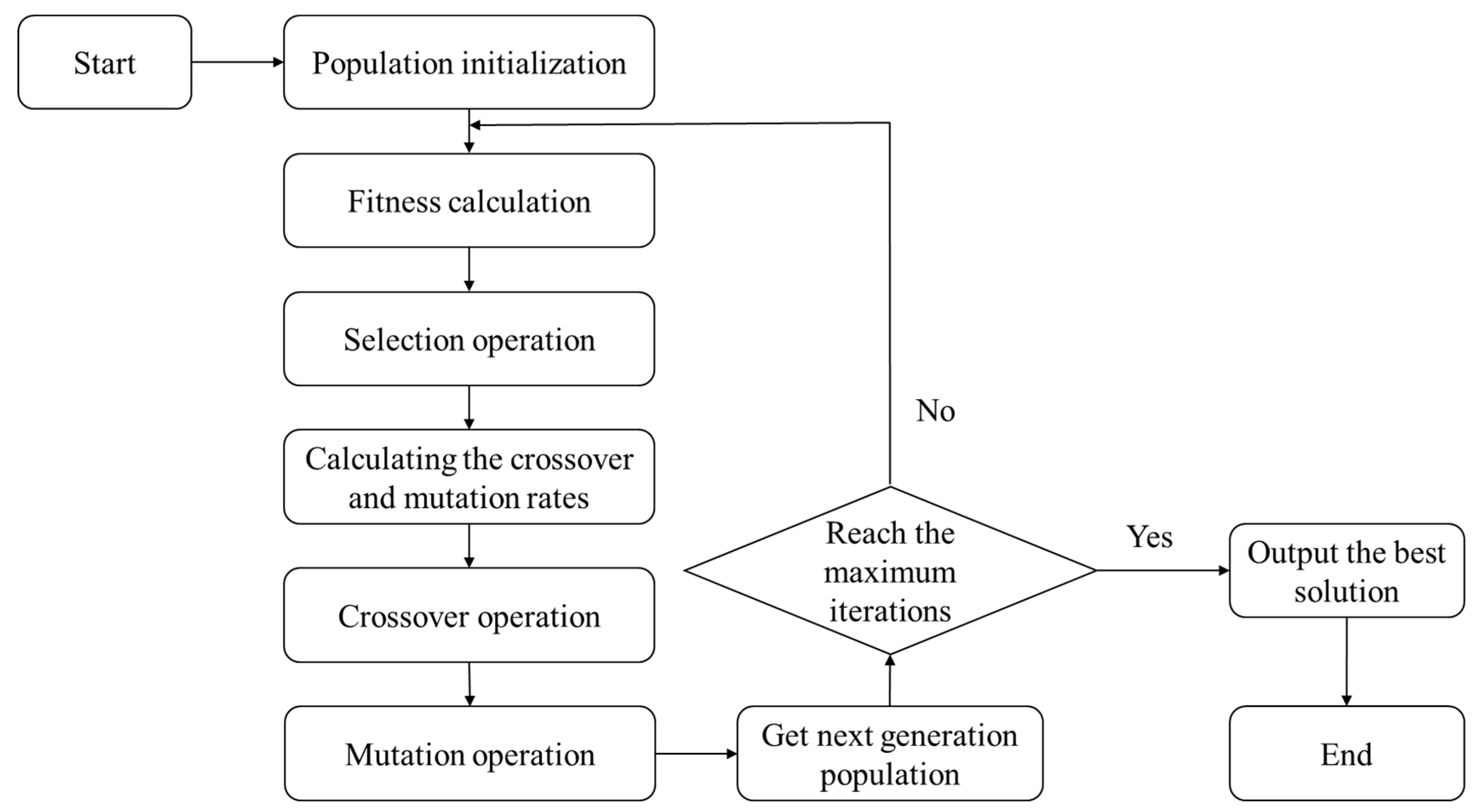
In this study, we propose a modified genetic algorithm based on the Spearman correlation coefficient. Generally, in GA, the probabilities of crossover and mutation operations are preset by experience, and all the genes have the same crossover and mutation rates. It is not conducive to the preservation of dominant genes. SGA determines the crossover and mutation rates by calculating the Spearman correlation coefficient instead of the rates, like GA does by experience. It is helpful for SGA to converge to the optimal solution quickly. As shown in Figure 1, the workflow of SGA is as follows:
Step 1 Population initialization: The population is composed of several individuals. Each individual has a chromosome with some genes, and each gene represents a fracturing parameter of the shale gas fracturing horizontal well. Thus, the population initialization process generates a certain number of individuals, recorded n, by randomly generating the fracturing parameters.
Step 2 Fitness calculation: Fitness is a standard to measure the quality of individuals, which is necessary for individual selection. In this study, the 30-day cumulative gas production obtained by the trained XGBoost model was used as the fitness. The greater the cumulative gas production, the higher the individual’s fitness.
Step 3 Selection operation: This step mainly selects n pairs of individuals from the population as parents, which are used to obtain the next generation via crossover and mutation operation. In this process, each individual has a probability to decide whether to be selected, which is decided by fitness. Generally, the greater the fitness, the bigger the selection probability. It is beneficial to maintain the superiority of the population.
Step 4 Calculating the crossover and mutation rates: This step is to obtain crossover and mutation rates based on the correlation coefficients of the fracturing parameters and the cumulative gas production.
Firstly, the Spearman correlation coefficient needs to be calculated. Correlation coefficients, such as Spearman, Pearson, and Kendall, are mainly used to describe the correlation between two parameters. The Pearson correlation coefficient is usually used for continuous variables with positive distribution and works well only with linear relationships. Nevertheless, the relationships between the fracturing parameters and the cumulative gas production are usually nonlinear. The Kendall correlation coefficient is applied to the rank variables. The Spearman correlation coefficient converts the original variables into the rank variables and obtains the correlation coefficient by Equation (2). The Spearman correlation coefficient can calculate the correlation between two variables with linear or even partial nonlinear correlation and has no requirement for data distribution. Therefore, the Spearman correlation coefficient is selected to calculate the correlative coefficients of the fracturing parameters and the cumulative gas production.
where is the Spearman correlative coefficient of the ith fracturing parameter, and n represents the number of samples. denotes the rank of the jth sample sorted according to the jth parameter, and is the mean rank of the samples sorted according to the ith fracturing parameter. denotes the rank of the jth sample sorted according to the cumulative gas production, and is the mean rank of the samples sorted according to the cumulative gas production. Generally, a more considerable absolute value of the Spearman correlative coefficient means a stronger correlation between the fracturing parameter and the cumulative gas production. However, a small value of the correlation coefficient does not mean the correlation must be weak. In other words, the correlation coefficient can only represent the importance of parameters to cumulative production to a certain extent. Nevertheless, the correlation coefficient is still an essential indicator for evaluating correlation.
Secondly, the crossover and mutation rates could be obtained based on the calculated Spearman correlation coefficients. We decide to give the genes with high Spearman correlative coefficients low crossover and mutation rates, which are conducive to preserving the superior genes of individuals. However, genes with high rates do not necessarily mean they will cross or mutate. Genes with low rates may also cross and mutate. It still retains some randomness, which is conducive to ensuring the diversity of the population and jumping out of the local optimum. The crossover and mutation rates could be obtained by Equation (3):
where denotes the crossover and mutation rates of the ith gene, and m is the number of fracturing parameters. A is the control factor, which could limit the crossover and mutation rates. Mostly, crossover and mutation operations have different values of a, and the mutation rates are far lower than the crossover rates.
Step 5 Crossover operation: Crossover operation aims to generate new individuals by crossing one or more genes on two chromosomes based on the calculated crossover rates. In this process, the genes with high crossover rates are more likely to be selected to cross, but not necessarily. It is conducive to preserving dominant genes while ensuring diversity.
Step 6 Mutation operation: The new individuals obtained by crossover operation must be implemented in the mutation operation to obtain the next generation population. The mutation randomly changes the fracturing parameter values corresponding to the chromosome genes. Similar to crossover operation, the genes with high mutation rates are more likely to be selected to achieve the mutation operation.
Step 7 Output the best solution: The next generation population could be obtained after Crossover and mutation operations. Then, the next step is judging whether it reaches the maximum iterations. If reached, the individual with the best fitness will be outputted as the best solution. If not, this new generation population will return to Step 2.
3. Application
3.1. Data Description
In this study, CMG commercial numerical simulation software was used to simulate shale gas multistage fracturing horizontal well development to obtain the geological, fracturing and production data, which could be used to build the production prediction model. For the production prediction model, the input consists of geological parameters, including porosity and permeability, and fracturing parameters, including the number of fracturing sections, the length of the horizontal well, fracture width and fracture half-length. Furthermore, the output is the cumulative gas production in 30 days. As shown in Figure 2, the shale gas reservoir established by CMG has a dimension of 3000 × 3000 × 100 m. The grid size is 200 × 200 × 10, wherein the grid step size in the I direction and J direction is 15 m, and that in the K direction is 10 m. The pertinent reservoir information is shown in Table 1. Moreover, the shale gas horizontal well is established in the fifth layer, and the fractures produced by perforation are vertical.
Producing the data takes three steps. First, the geological and fracturing parameters are produced randomly in the reasonable value ranges, shown in Table 2. Second, these parameters are inputted into the above CMG numerical model for simulation calculation to obtain the 30-day cumulative gas production of the horizontal well. Third, the dataset is obtained by repeating the two steps. In this study, the process was repeated by programming, and a dataset with 500 groups of samples was obtained. Figure 3 gives the distributions between input parameters and 30-day cumulative gas production.
3.2. Building the Productivity Prediction Model
This paper uses the XGBoost algorithm to establish the production prediction model for fracturing horizontal wells. Six parameters, including porosity, permeability, the number of fracturing sections, the length of the horizontal well, fracture width and fracture half-length, were used as the input of the production prediction model of fracturing horizontal wells. Furthermore, the output is the 30-day cumulative gas production. Then, 80% of the samples from the dataset above were randomly selected as the training set, and the remaining 20% were used as the testing set. In addition, 10% of samples from the training set were used as the validation set to achieve cross-validation. The training set was used to train the production prediction model based on the XGBoost algorithm. Moreover, the hyperparameter combination of the XGBoost model was optimized with the grid search method, and the results are shown in Table 3. In the process, the average Mean Absolute Errors (MAEs) of cross-validation is 3.68%, which shows that the XGBoost model has a low training error.
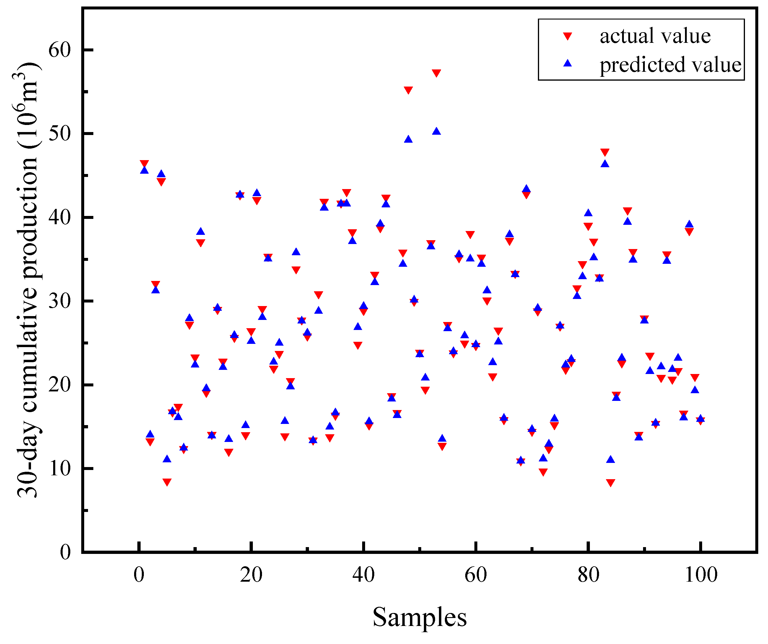
In addition, the samples in the testing set were used to validate the prediction performance of the trained XGBoost model. The geological and fracturing parameters of the samples in the testing set were inputted into the trained XGBoost model, and the predicted cumulative gas productions were obtained. Figure 4 gives the comparison plot of the predicted and actual cumulative gas productions. From the plot, it can be seen that the predicted values are close to the actual values. More precisely, the MAE was calculated to show the performance of the trained XGBoost model in the testing set, and the value is 4.06%. Moreover, R2, a standard statistical indicator, was used to show the prediction accuracy of the XGBoost model, and the value is 0.9811. Both indicators show that the trained XGBoost model performs excellently in predicting cumulative gas production. Therefore, the trained XGBoost model can replace the numerical model for the fracturing parameter optimization.
3.3. Fracturing Parameters Optimization
The purpose of fracturing parameters optimization is to find the optimal fracturing parameter combination with the maximum cumulative gas production based on the production prediction model. However, in this study, the trained XGBoost model’s input parameters include geological and fracturing parameters. To optimize the fracturing parameters, the geological parameters should be determined first, and then the optimization algorithm is used to optimize the fracturing parameters. Thus, nine production prediction models with determined geological parameters were used for the fracturing parameter optimization tests. In the process, we optimized the fracturing parameters with three optimization methods: GA, SGA, and Stochastic Gradient Descent (SGD), a classical gradient-based optimization algorithm. For SGA, the mutation and crossover rates were calculated first, and the control factors of the crossover operation and the mutation operation are 50% and 20%, respectively. The results are shown in Table 4. In addition, for GA, the mutation rate was 15%, and the crossover rate was 30%. Moreover, for GA and SGA, the population size was 20, and the maximum iterations were 100. Figure 5 gives the comparison plots of the optimization results of GA, SGA and SGD. The nine comparison plots show that the number of iteration steps required for SGA to search the optimal value is less than GA, and SGA’s optimization results are a little higher than GA’s. It can be seen that SGA has obvious advantages in optimization speed. Moreover, SGD has a much faster speed than SGA thanks to less computation per iteration. Nevertheless, SGA has obviously higher accuracy in fracturing parameter optimization than SGD. Furthermore, the optimization results of SGA show significant diversity in different porosity and permeability conditions, as shown in Table 5.
Although SGA has an excellent performance in fracturing parameter optimization, it still has some limitations. First, calculating the Spearman correlation coefficient has specific requirements with regards to the quantity and quality of the dataset. Second, the Spearman correlation coefficient can only show a partial nonlinear relationship and roughly represent the correlation, which might limit the optimization accuracy.
3.4. Robustness Analysis
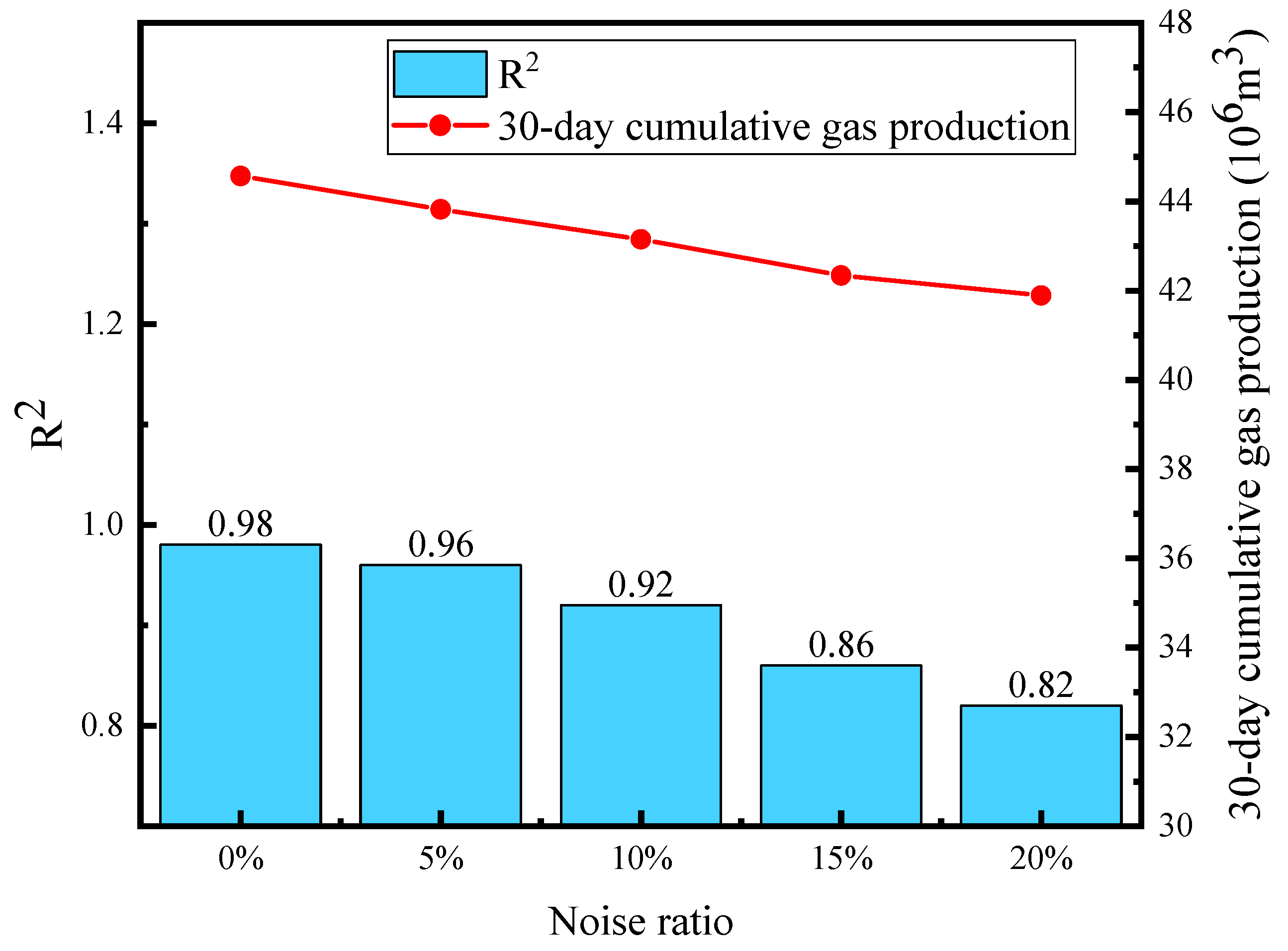
Robustness analysis is a common way to test the stability of methods. This paper will test the stability of this method by adding Gaussian noise to the dataset. As shown in Figure 6, with the increasing noise, the R2 of the XGBoost model is also decreasing. When we add Gaussian noise to 20%, the R2 of the XGBoost model can still exceed 0.8. It shows that the XGBoot model has specific stability. In addition, we can find that the optimal cumulative gas productions obtained by the XGBoost model and SGA are generally decreasing with the noise increasing. However, as can be seen, the drop in the optimal cumulative gas production does not exceed 3 × 10⁶ m3 when the noise increases to 20%. It is acceptable and shows that SGA is relatively stable.
4. Conclusions and Future Research
In this study, we propose a modified algorithm based on the Spearman correlation coefficient to rapidly optimize the fracturing parameters of shale gas horizontal wells. The proposed method could speed up the search for the optimal solution by improving the crossover and mutation operations based on the Spearman correlation coefficient. The main improvement is changing the crossover and mutation rates in accordance with correlation, which results in retaining the dominant genes in the optimization process. Before testing the performance of SGA, a production prediction model is built by the XGBoost algorithm based on the dataset obtained by simulating the production process of shale gas fracturing horizontal wells. The test results show that the XGBoost model performs well in predicting the 30-day cumulative gas production. Based on the trained XGBoost model, SGA is used to optimize the fracturing parameters with the 30-day cumulative production as the optimization objective. The optimization results show that SGA has a faster optimization speed than GA and higher accuracy than SGD. However, SGA still has two limitations. On the one hand, calculating the Spearman correlation coefficient has specific requirements from the quantity and quality of the dataset. On the other hand, the Spearman correlation coefficient can only roughly represent the correlation, which might limit the optimization accuracy.
In future research, we will expand our study based on the following two aspects. First, the data we used in this study is from the numerical simulation by CMG commercial numerical simulation software. However, more parameters could be considered in the oilfield than those in the numerical simulation. Hence, an extension of the proposed method is that SGA can be used in the horizontal well fracturing optimization in the oilfield. It can also further test the applicability of SGA. Second, the Spearman correlation coefficient can only roughly represent the correlation. It might have a slight impact on the population quality obtained by crossing and variation operations. Thus, another extension is to select appropriate methods to improve the efficiency of crossover and mutation operations.
Author Contributions
X.Z.: Conceptualization, Methodology, Software, Testing, Formal analysis, Investigation, Data curation, Experimental studies, Writing—Original draft preparation, Writing—Reviewing and Editing. Q.R.: Conceptualization, Resources, Data curation, Data acquisition, Writing—Original draft preparation, Writing—Reviewing and Editing, Visualization, Supervision, Project administration. All authors have read and agreed to the published version of the manuscript.
Funding
This research was funded by [Scientific Research and Technology Development Project of PetroChina Company Limited] grant number [2020B-4911]. And the APC was funded by [Research Institute of Petroleum Exploration and Development].
Data Availability Statement
Data is available.
Acknowledgments
The authors declared that they have no conflicts of interest in this work. The authors greatly appreciate the support from the fund named Scientific Research and Technology Development Project of PetroChina Company Limited (Grant NO. 2020B-4911).
Conflicts of Interest
The authors declare no conflict of interest.
Nomenclature
| Acronyms | |
| a | the control factor |
| d | the ranks of fracturing parameters |
| the mean values of fracturing parameters’ ranks | |
| GA | Genetic Algorithm |
| l | the loss function of XGBoost |
| MAE | Mean Absolute Error |
| m | the number of fracturing parameters |
| n | the number of samples |
| r | the crossover and mutation rates |
| s | the ranks of the cumulative gas productions |
| the mean value of the cumulative gas productions’ ranks | |
| SGA | the modified Genetic Algorithm combined with the Spearman correlative coefficient |
| SGD | Stochastic Gradient Descent |
| XGBoost | Extreme Gradient Boosting |
| y | the actual value of cumulative gas production |
| the predicted value of XGBoost | |
| ρ | the spearman correlative coefficient of fracturing parameter |
References
- Reymond, M. European key issues concerning natural gas: Dependence and vulnerability. Energy Policy 2007, 35, 4169–4176. [Google Scholar] [CrossRef]
- Barnes, R.; Bosworth, R. LNG is linking regional natural gas markets: Evidence from the gravity model. Energy Econ. 2015, 47, 11–17. [Google Scholar] [CrossRef]
- Najibi, H.; Rezaei, R.; Javanmardi, J.; Nasrifar, K.H.; Moshfeghian, M. Economic evaluation of natural gas transportation from Iran’s South-Pars gas field to market. Appl. Therm. Eng. 2009, 29, 2009–2015. [Google Scholar] [CrossRef]
- Wang, T.; Lin, B.Q. Impacts of unconventional gas development on China’s natural gas production and import. Renew. Sustain. Energy Rev. 2014, 39, 546–554. [Google Scholar] [CrossRef]
- Song, Y.; Li, Z.; Jiang, Z.X.; Luo, Q.; Liu, D.D.; Gao, Z.Y. Progress and development trend of unconventional oil and gas geological research. Pet. Explor. Dev. 2017, 44, 675–685. [Google Scholar] [CrossRef]
- Umbach, F. The unconventional gas revolution and the prospects for Europe and Asia. Asia Eur. J. 2013, 11, 305–322. [Google Scholar] [CrossRef]
- Guo, X.S.; Hu, D.F.; Li, Y.P.; Wei, Z.H.; Wei, X.F.; Liu, Z.J. Geological factors controlling shale gas enrichment and high production in Fuling shale gas field. Pet. Explor. Dev. 2017, 44, 513–523. [Google Scholar] [CrossRef]
- Zhang, X.T.; Jiang, X.; Yang, J.Y.; Chen, M. A Newly Developed Rate Analysis Method for a Single Shale Gas Well. Energy Explor. Exploit. 2015, 33, 309–316. [Google Scholar] [CrossRef] [Green Version]
- Xiang, Z.P.; Liang, H.B.; Qi, Z.L.; Xiao, Q.H.; Yan, W.D.; Liang, B.S.; Guo, Q.T. Mathematical Model for Isothermal Adsorption of Supercritical Shale Gas. J. Porous Media 2019, 22, 499–510. [Google Scholar] [CrossRef]
- Liang, X.; Lou, J.S.; Zhang, Y.Q.; Zhang, J.H.; Zhang, L.; Song, J.; Parlindungan, M.H.; Rana, K.H.; Dai, G.Y.; Amarjit, S.B. The First Real Time Reservoir Characterization, Well Placement and RSS Applications in Shale Gas Horizontal Well Play in Central China—A Case Study. In Proceedings of the IADC/SPE Asia Pacific Drilling Technology Conference and Exhibition, Tianjin, China, 19 July 2012. Paper Number: SPE-156239-MS. [Google Scholar] [CrossRef]
- Wang, G.; Zhou, H.; Fan, H.; Si, N.; Liu, J.; Ma, D.; Pan, W. Utilising Managed Pressure Drilling to Drill Shale Gas Horizontal Well in Fuling Shale Gas Field. In Proceedings of the SPE Asia Pacific Oil & Gas Conference and Exhibition, Perth, Australia, 17–19 October 2016. Paper Number: SPE-182490-MS. [Google Scholar] [CrossRef]
- Lin, R.; Ren, L.; Zhao, J.Z. Cluster Spacing Optimization for Horizontal-Well Fracturing in Shale Gas Reservoirs: Modeling and Field Application. In Proceedings of the SPE Europec featured at 80th EAGE Conference and Exhibition, Copenhagen, Denmark, 5–8 June 2018. Paper Number: SPE-190775-MS. [Google Scholar] [CrossRef]
- Reddy, R.M.; Rao, B.N. Fractal finite element method based shape sensitivity analysis of mixed-mode fracture. Finite Elem. Anal. Des. 2008, 44, 875–888. [Google Scholar] [CrossRef]
- Fu, J.L.; Wen, X.H. A Regularized Production-Optimization Method for Improved Reservoir Management. SPE J. 2018, 23, 467–481. [Google Scholar] [CrossRef]
- Atefeh, J.; Behnam, J. Stochastic Oilfield Optimization Under Uncertain Future Development Plans. SPE J. 2019, 24, 1526–1551. [Google Scholar] [CrossRef]
- Lin, R.; Li, G.M.; Zhao, J.Z.; Ren, L.; Wu, J.F. Productivity model of shale gas fractured horizontal well considering complex fracture morphology. J. Pet. Sci. Eng. 2022, 208, 109511. [Google Scholar] [CrossRef]
- Yuan, Y.Z.; Yan, W.D.; Chen, F.B.; Li, J.Q.; Xiao, Q.H.; Huang, X.L. Numerical Simulation for Shale Gas Flow in Complex Fracture System of Fractured Horizontal Well. Int. J. Nonlinear Sci. Numer. Simul. 2018, 19, 367–377. [Google Scholar] [CrossRef]
- Chen, X.C.; Li, J.; Gao, P.; Zhou, J.C. Prediction of shale gas horizontal wells productivity after volume fracturing using machine learning—an LSTM approach. Pet. Sci. Technol. 2022, 40, 1861–1877. [Google Scholar] [CrossRef]
- Wang, T.Y.; Wang, Q.S.; Shi, J.; Zhang, W.H.; Ren, W.X.; Wang, H.Z.; Tian, S.C. Productivity Prediction of Fractured Horizontal Well in Shale Gas Reservoirs with Machine Learning Algorithms. Appl. Sci. 2022, 11, 12064. [Google Scholar] [CrossRef]
- Xue, L.; Liu, Y.T.; Xiong, Y.F.; Liu, Y.L.; Cui, X.H.; Lei, G. A data-driven shale gas production forecasting method based on the multi-objective random forest regression. J. Pet. Sci. Eng. 2021, 196, 107801. [Google Scholar] [CrossRef]
- Al-Fatlawi, O.; Hossain, M.; Essa, A. Optimization of Fracture Parameters for Hydraulic Fractured Horizontal Well in a Heterogeneous Tight Reservoir: An Equivalent Homogeneous Modelling Approach. In Proceedings of the SPE Kuwait Oil & Gas Show and Conference, Mishref, Kuwait, 15–18 October 2019. Paper Number: SPE-198185-MS. [Google Scholar] [CrossRef]
- Wei, Z.P.; Wang, J.W.; Liu, R.M.; Wang, T.; Han, G.N. Parameter Optimization of Segmental Multicluster Fractured Horizontal Wells in Extremely Rich Gas Condensate Shale Reservoirs. Econ. Geol. 2021, 9, 730080. [Google Scholar] [CrossRef]
- Chen, Z.M.; Chen, D.; Li, W.Y.; He, Y.X.; Li, D.X.; Wang, J.N. A Parameter Optimization Workflow of Fractured Horizontal Well in Unconventional Reservoir: Case Study. In Proceedings of the International Petroleum Technology Conference, Riyadh, Saudi Arabia, 21–23 February 2022. Paper Number: IPTC-22215-MS. [Google Scholar] [CrossRef]
- Xu, S.Q.; Feng, Q.H.; Wang, S.; Javadpour, F.; Li, Y.Y. Optimization of multistage fractured horizontal well in tight oil based on embedded discrete fracture model. Comput. Chem. Eng. 2018, 117, 291–308. [Google Scholar] [CrossRef]
- Zhang, L.; Li, Z.P.; Lai, F.P.; Li, H.; Adenutsi, C.D.; Wang, K.J.; Yang, S.; Xu, W.L. Integrated optimization design for horizontal well placement and fracturing in tight oil reservoirs. J. Pet. Sci. Eng. 2019, 178, 82–96. [Google Scholar] [CrossRef]
- Wang, L.; Yao, Y.D.; Wang, K.J.; Adenutsi, C.D.; Zhao, G.X.; Lai, F.P. Data-driven multi-objective optimization design method for shale gas fracturing parameters. J. Nat. Gas Sci. Eng. 2022, 99, 104420. [Google Scholar] [CrossRef]
- Jiang, B.B.; Li, H.T.; Zhang, Y.; Wang, Y.Q.; Wang, J.C.; Patil, S. Multiple fracturing parameters optimization for horizontal gas well using a novel hybrid method. J. Nat. Gas Sci. Eng. 2016, 34, 604–615. [Google Scholar] [CrossRef]
- Ma, C.X.; Xing, Y.; Qu, Y.Q.; Cheng, X.; Wu, H.N.; Luo, P.; Xu, P.X. A New Fracture Parameter Optimization Method for the Horizontal Well Section of Shale Oil. Econ. Geol. 2022, 10, 895382. [Google Scholar] [CrossRef]
- Bian, X.B.; Ding, S.D.; Jiang, T.X.; Li, S.M.; Wang, H.T.; Wei, R.; Xiao, B.; Su, Y.; Zhong, G.Y.; Zuo, L.; et al. A Comprehensive Optimization Method of Multi Fracturing Parameters for Shale Gas Well Factory. In Proceedings of the 54th U.S. Rock Mechanics/Geomechanics Symposium, Physical Event Cancelled, Golden, CO, USA, 28 June–1 July 2020. Paper Number: ARMA-2020-1660. [Google Scholar]
- Vazquez, O.; Ross, G.; Jordan, M.M.; Baskoro, D.A.A.; Mackay, E.; Johnston, C.; Strachan, A. Automatic Optimization of Oilfield-Scale-Inhibitor Squeeze Treatments Delivered by Diving-Support Vessel. SPE J. 2018, 24, 60–70. [Google Scholar] [CrossRef]
- Dong, Z.; Wu, L.; Wang, L.; Li, W.; Wang, Z.; Liu, Z. Optimization of Fracturing Parameters with Machine-Learning and Evolutionary Algorithm Methods. Energies 2022, 15, 6063. [Google Scholar] [CrossRef]
- Guo, D.L.; Kang, Y.W.; Wang, Z.Y.; Zhao, Y.X.; Li, S.G. Optimization of fracturing parameters for tight oil production based on genetic algorithm. Petroleum 2022, 8, 252–263. [Google Scholar] [CrossRef]
- Yao, J.; Li, Z.H.; Liu, L.J.; Fan, W.P.; Zhang, M.S.; Zhang, K. Optimization of Fracturing Parameters by Modified Variable-Length Particle-Swarm Optimization in Shale-Gas Reservoir. SPE J. 2021, 26, 1032–1049. [Google Scholar] [CrossRef]
- Zhou, J.; Hua, Z.S. A correlation guided genetic algorithm and its application to feature selection. Appl. Soft Comput. 2022, 123, 108964. [Google Scholar] [CrossRef]
- Chen, T.; Guestrin, C. XGBoost: A Scalable Tree Boosting System. In Proceedings of the 22nd ACM SIGKDD International Conference on Knowledge Discovery and Data Mining (KDD), San Francisco, CA, USA, 13–17 August 2016. [Google Scholar]
- Tang, J.Z.; Fan, B.; Xiao, L.Z.; Tian, S.C.; Zhang, F.S.; Zhang, L.Y.; Weitz, D. A New Ensemble Machine-Learning Framework for Searching Sweet Spots in Shale Reservoirs. SPE J. 2021, 26, 482–497. [Google Scholar] [CrossRef]
- Carpenter, C. Dynamometer-Card Classification Uses Machine Learning. J. Pet. Technol. 2020, 72, 52–53. [Google Scholar] [CrossRef]
- Liu, W.; Liu, W.D.; Gu, J.W. Predictive model for water absorption in sublayers using a Joint Distribution Adaption based XGBoost transfer learning method. J. Pet. Sci. Eng. 2020, 188, 106937. [Google Scholar] [CrossRef]
- Zhai, L.Z.; Feng, S.H. A novel evacuation path planning method based on improved genetic algorithm. J. Intell. Fuzzy Syst. 2022, 42, 1813–1823. [Google Scholar] [CrossRef]
- Wang, Z.Y.; Bai, W.L.; Liu, H. An optimized finite-difference scheme based on the improved PSO algorithm for wave propagation. In Proceedings of the SEG International Exposition and Annual Meeting, San Antonio, TX, USA, 15–20 September 2019. Paper Number: SEG-2019-3216363. [Google Scholar]
- John, H. Adaptation in Natural and Artificial Systems; MIT Press: Cambridge, MA, USA, 1992; ISBN 978-0262581110. [Google Scholar]
- Zhang, T.Y.; Zhang, Q.F.; Zhao, Z.N.; Cheng, L.; Liu, G.J. Optimization of boiler’s convection tubes based on Genetic Algorithm. In Proceedings of the 4th International Conference on Electrical and Electronics Engineering and Computer Science (ICEEECS), Jinan, China, 15–16 October 2016. [Google Scholar]
- Ding, K.; Ni, Y.; Fan, L.F.; Sun, T.L. Optimal Design of Water Supply Network Based on Adaptive Penalty Function and Improved Genetic Algorithm. Math. Probl. Eng. 2022, 2022, 8252086. [Google Scholar] [CrossRef]
- Li, H.; Shi, N.Y. Application of Genetic Optimization Algorithm in Financial Portfolio Problem. Comput. Intell. Neurosci. 2022, 2022, 5246309. [Google Scholar] [CrossRef]
Figure 1.
The workflow of SGA.

Figure 2.
Numerical simulation of the shale gas fracturing horizontal well.

Figure 3.
The distribution plots between the input parameters and output parameters.

Figure 4.
Comparison plots of actual values vs. predicted values for the testing samples. The blue triangles denote the predicted values, and the red inverted triangles represent the actual values.
Figure 4.
Comparison plots of actual values vs. predicted values for the testing samples. The blue triangles denote the predicted values, and the red inverted triangles represent the actual values.

Figure 5.
Comparison plots of GA, SGA, and SGD. The light-blue line denotes the optimization process of GA, and the red line represents the optimization process of SGA. The blue line is the optimization process of SGD. (a–i) denote the optimization results of the production prediction models with different porosities and permeabilities.

Figure 6.
The results of robustness tests. The red points denote the optimization results of SGA in the different tests. The blue columns represent the R2 of the XGBoost models in the five tests.
Figure 6.
The results of robustness tests. The red points denote the optimization results of SGA in the different tests. The blue columns represent the R2 of the XGBoost models in the five tests.


Table 1.
Basic gas reservoir parameters.
| Basic Parameters | Value | Units |
|---|---|---|
| Initial reservoir pressure | 28.9 | Mpa |
| Total production time | 30 | day |
| Depth to the tops of grid blocks | 2890 | m |
| Depth to water–gas contact | 4500 | m |
Table 2.
The values of input parameters.
| Input Parameters | Units | Value | |
|---|---|---|---|
| Geological parameters | Porosity | % | 5–15 |
| Permeability | mD | 0.0001–0.001 | |
| Fracturing parameters | The number of fracturing sections | \ | 10–30 |
| The length of the horizontal well | m | 300–3000 | |
| Fracture width | m | 50–250 | |
| Fracture half-length | m | 0.001–0.005 | |
Table 3.
Summary of optimal hyperparameter settings for the XGBoost model.
| Hyperparameters | Value |
|---|---|
| booster | gbtree |
| n_estimators | 150 |
| max_depth | 12 |
| min_child_weight | 9 |
| eta | 0.023 |
| gamma | 0.15 |
| subsample | 1 |
Table 4.
The mutation and crossover rates of each fracture parameter.
| Fracturing Parameters | Spearman Correlative Coefficient | Crossover Rate (%) | Mutation Rate (%) |
|---|---|---|---|
| the number of fracturing sections | 0.794 | 29.6 | 11.84 |
| the length of the horizontal well | 0.525 | 36.51 | 14.6 |
| fracture width | 0.356 | 40.85 | 16.34 |
| fracture half-length | 0.271 | 43.04 | 17.21 |
Table 5.
The optimal fracturing parameters of the nine test samples.
| Test Samples | Geological Parameters | The Optimal Fracturing Parameters | ||||
|---|---|---|---|---|---|---|
| Permeability (mD) | Porosity (%) | The Number of Fracturing Sections | The Length of the Horizontal Well (m) | Fracture Width (m) | Fracture Half-Length (m) | |
| (a) | 0.00012 | 14.8 | 29 | 870 | 0.00478 | 229.95 |
| (b) | 0.0005 | 14.8 | 29 | 2325 | 0.00475 | 207.43 |
| (c) | 0.00098 | 14.8 | 29 | 1905 | 0.00415 | 192.37 |
| (d) | 0.00012 | 10 | 28 | 2490 | 0.00476 | 244.72 |
| (e) | 0.0005 | 10 | 28 | 2685 | 0.00461 | 218.92 |
| (f) | 0.00098 | 10 | 28 | 2715 | 0.00447 | 181.62 |
| (g) | 0.00012 | 5.2 | 28 | 2370 | 0.00496 | 242.35 |
| (h) | 0.0005 | 5.2 | 29 | 1320 | 0.00484 | 228.5 |
| (i) | 0.00098 | 5.2 | 28 | 1680 | 0.00488 | 229.21 |
Disclaimer/Publisher’s Note: The statements, opinions and data contained in all publications are solely those of the individual author(s) and contributor(s) and not of MDPI and/or the editor(s). MDPI and/or the editor(s) disclaim responsibility for any injury to people or property resulting from any ideas, methods, instructions or products referred to in the content. |
© 2023 by the authors. Licensee MDPI, Basel, Switzerland. This article is an open access article distributed under the terms and conditions of the Creative Commons Attribution (CC BY) license (https://creativecommons.org/licenses/by/4.0/).
Share and Cite
MDPI and ACS Style
Zhou, X.; Ran, Q. Optimization of Fracturing Parameters by Modified Genetic Algorithm in Shale Gas Reservoir. Energies 2023, 16, 2868. https://0-doi-org.brum.beds.ac.uk/10.3390/en16062868
AMA Style
Zhou X, Ran Q. Optimization of Fracturing Parameters by Modified Genetic Algorithm in Shale Gas Reservoir. Energies. 2023; 16(6):2868. https://0-doi-org.brum.beds.ac.uk/10.3390/en16062868
Chicago/Turabian StyleZhou, Xin, and Qiquan Ran. 2023. "Optimization of Fracturing Parameters by Modified Genetic Algorithm in Shale Gas Reservoir" Energies 16, no. 6: 2868. https://0-doi-org.brum.beds.ac.uk/10.3390/en16062868
Note that from the first issue of 2016, this journal uses article numbers instead of page numbers. See further details here.