
Wind Forecast at Medium Voltage Distribution Networks

1
Department of Electrical and Computer Engineering, Instituto Superior Técnico—IST, Universidade de Lisboa, 1049-001 Lisbon, Portugal
2
INESC-ID—Instituto de Engenharia de Sistemas e Computadores-Investigação e Desenvolvimento, 1000-029 Lisboa, Portugal
*
Author to whom correspondence should be addressed.
Energies 2023, 16(6), 2887; https://0-doi-org.brum.beds.ac.uk/10.3390/en16062887
Submission received: 16 February 2023
/
Revised: 12 March 2023
/
Accepted: 17 March 2023
/
Published: 21 March 2023
(This article belongs to the Special Issue Distribution Grids Modernization II)
Abstract
:Due to the intermittent and variable nature of wind, Wind Power Generation Forecast (WPGF) has become an essential task for power system operators who are looking for reliable wind penetration into the electric grid. Since there is a need to forecast wind power generation accurately, the main contribution of this paper is the development, implementation, and comparison of WPGF methods in a framework to be used by distribution system operators (DSOs). The methodology applied comprised five stages: pre-processing, feature selection, forecasting models, post-processing, and validation, using the historical wind power generation data (measured at secondary substations) of 20 wind farms connected to the medium voltage (MV) distribution network in Portugal. After comparing the accuracy of eight different models in terms of their relative root mean square error (RRMSE), extreme gradient boosting (XGBOOST) appeared as the best-suited forecasting method for wind power generation. The best average RRMSE achieved by the proposed XGBOOST model for 1-year training (January–December of 2020) and 6 months forecast (January–June of 2021) corresponds to 13.48%, outperforming the predictions of the Portuguese DSO by 20%.
1. Introduction
1.1. Motivation
Nowadays, the world is going through an energy transition process from fossil fuels to renewable energies, which aims to reduce the environmental impact of the energy sector. To increase the penetration rate of Renewable Energy Sources (RES) in power systems, significant incentive schemes and policies have been considered by governments. The European Union (EU), under the 2030 climate and energy framework for the period 2021–2030, is part of the ambitious European Green Deal. The framework commits the EU to reducing greenhouse emissions by at least 40% (as compared to 1990 levels), to increase the amount of renewable energy in the energy mix by at least 32%, and to improve the energy efficiency by at least 32.5% [1]. To achieve those targets, a high penetration of RES such as solar, wind, hydropower, geothermal, biomass, biofuels, waves, or tidal is necessary.
Over the last years, a rapid expansion of Solar Photovoltaic (PV) and wind has been seen, mainly because the cost of PV and because wind power installations have declined sharply. Out of all the available RES, PV and wind are considered now to be the most abundant, developed, economically viable, and commercially accepted types worldwide [2]. Without considering hydropower, wind is a renewable resource, with a higher installed capacity. According to the Global Wind Report 2021 [3], the year 2020 was the best year in history for the global wind industry. The report shows a year-over-year growth of 53%, considering that for 2020, more than 93 GW of wind power was installed, with 86.9 GW allocated to the onshore market and 6.1 GW to the offshore market. The new installations bring the global cumulative wind power capacity up to 743 GW [3].
However, the uncertainty in wind power generation is very large due to the inherent variability of wind speed [4,5]. Hence, wind variability needs to be understood by operators of power systems and wind farms in order to ensure that supply and demand are balanced, and that the power network operates without constraints. Since supply and demand should be equal at all times but wind power generation depends on the availability of wind, which is a weather-dependent source, the integration into the existing electricity supply system brings some challenges at the level of secondary substations that need to be addressed by DSOs of power networks [6,7].
Some of the challenges include system stability and reliability, due to grid congestion or the intermittency of supply; system balance, which requires a strong information exchange between the DSO and the Transmission System Operator (TSO), or flexibility services (voltage support and demand-side response) to ensure that the network is stabilized amid the varying energy generation and consumption. Other challenges that are associated with optimizing the grid include technical imbalances in the existing equipment, and saturations in the MV network or in the substations [8].
This is where WPGF appears as one of the most efficient ways to overcome some of these problems, and to help power system operators to reduce the risk of unreliable electricity supply. The development of new techniques to improve the understanding of wind power generation, through simulation, forecasting, distribution curve fitting, filtering, and modeling, allows better decisions to be made about the expansion of the wind sector and the better management of the electricity system [9].
WPGF accuracy is directly connected to the need for balancing energy, and therefore, to the cost of wind power integration [10]. Accurate estimations of wind speed and wind power generation might improve safety, reliability, and profitability [9] not only in the operation of the wind farms, but also in the secondary substations managed by DSOs.
Consequently, a large amount of research has been directed towards the development and improvement of good and reliable wind forecasts in recent years, and different forecast systems have been developed.
1.2. State of the Art on Wind Power Forecast Methods
WPGF has been a topic of interest for many researchers, due to the importance of integrating RES into the power system and all the implications that it brings. Based on an analysis of the literature, wind forecast methods can be divided into six overall groups: persistence method, physical methods, statistical methods, Artificial Neural Networks (ANNs)-based models, hybrid methods, and new models.
The persistence method uses the simple assumption that the value at a certain future time will be the same as it is when the forecast is made. It is based on the assumption of a high correlation between present and future values, and produces accurate predictions for very-short-term forecasts [11]. As expected, the accuracy of this model degrades rapidly with the increasing prediction lead time [12], so it is normally used as a reference to evaluate the performance of advanced methods.
Physical methods use forecast values from a Numerical Weather Prediction (NWP) model as an input to calculate the wind power generation based on the power curve. The NWP method is mathematically complex and is usually run on supercomputers because it requires a high computation time to produce forecasts, which limits its usefulness [12]. However, J.Taylor et al. [4] developed a new type of physical method to predict the probability density function of wind power generation for the 1 to 10 days ahead forecast using Weather Emsemble Predictions (WEPs). WEPs are generated from atmospheric models and consist of multiple scenarios for the future value of a weather variable (in this case, wind speed). The results of this study were compared with the statistical time series method, ARMA, and it was found that WEPs gave more accurate and comfortably superior results; therefore, the author mentions that WEPs have a strong potential for WPGF.
Statistical methods are based on training with measured data (time series). They are easy to model, capable of providing timely prediction and mostly used for short-term forecasting [12]. Several types of time series models may be considered, but the most popular are AR and its variants ARX, ARMA, and ARIMA. For instance, C.Gallego et al. [13] presents a study focused on modeling the influences of local wind speed and wind direction on the dynamics of a wind power time series, using a generalized linear AR model. What they found in their study is that the local measurements of both wind speed and wind direction provide useful information for a better comprehension of wind power time series dynamics, at least when considering the case of very-short-term forecasting. In particular, local wind direction contributes to the modeling of some features of the prevailing winds, such as the impact on wind variability, whereas the non-linearities related to the power transformation process can be introduced by considering the local wind speed. Another study made by M.Duran et al. [14], tested an ARX model for wind power prediction, using wind speed as an exogenous variable. The results for a 24 h time horizon showed a significant improvement in accuracy when comparing the mean error of their model with persistence and a traditional AR model. According to [14], when compared with AR, the improvement of ARX is about 14% and about 26% when compared with persistence.
ANNs are typically composed of nodes (or neurons) that are distributed across different layers, namely input, hidden, and output layers. Each node in a layer is linked to the ones in the next using a weight parameter that measures the strength of that connection [15]. ANNs can identify the non-linear relationships between the input features and the output data. There are several kinds of ANNs but the most common neural networks used for WPGF are Feed Forward Neural Networks (FFNNs), Back-Propagation Neural Networks (BPNNs) and Recurrent Neural Networks (RNNs), which also includes a more advanced version called the LSTM neural network. A successful application of ANNs in combination with wavelet transform for short-term wind power forecasting in Portugal is presented by J.Catalao in [16]. The model proposed predicts the value of wind power 3 h ahead, and it is compared with persistence, ARIMA, and another neural network approach. The results of the study confirmed that this model is effective, since the Mean Absolute Percentage Error (MAPE) has an average value of 6.97%, outperforming the other methods analyzed in [16]. In addition, the introduction of the wavelet transform enables a reduction in the error when compared with the normal neural network. Another model developed by M.Mabel et al. is presented in [17], to forecast the wind power generation of seven wind farms in Muppandal, India. In this case, a BPNN is implemented using three input variables: wind speed, relative humidity, and generation hours. The model accuracy is then evaluated by comparing the predicted power with the actual measured values, using two years of training and one year of the forecast. The results are satisfactory and in agreement, since the overall percentage error obtained was 4%.
Hybrid methods refer to the combination of different forecasting methods, with the aim of retaining the merits of each technique and improving the overall accuracy [18]. It includes the combination of physical and statistical methods, the combination of alternative statistical methods, or the combination of models for short-term and medium-term forecasting, for instance. Combining forecasting models does not always perform better than the best individual model; however, in some cases it is viewed as being less risky to combine forecasts than to select an individual forecast [19]. A recent study from S.Khazaei [20] presents a hybrid approach for short-term wind power forecasting using the historical data of Sotavento wind farm (located in Spain) and NWP data obtained from the Meteogalicia numerical weather forecast system. The goal of the study is to forecast the wind power for the next 24 h, which is carried out through three stages: wind direction forecast, wind speed forecast, and wind power forecast. In all three phases, the same hybrid method is used, and the only difference is in the input data set. Outlier detection, the decomposition of time series using wavelet transform, feature selection, and the prediction of each time series decomposed using a neural network constitute the main steps of the proposed method, and the results obtained demonstrate that it has a very high accuracy.
The last group corresponds to some novel wind forecast models that have been developed in recent years. Among the most interesting ones, the XGBOOST, Adaptative Neural Fuzzy Inference System (ANFIS), RF, and SVM models have achieved the most accurate predictions for wind power generation. For instance, in [21] a study from H.Zheng et al. proposes a model for short-term wind power generation forecast based on XGBOOST, with weather similarity analysis and feature engineering. Hourly wind power generation is predicted for the week between 21 and 28 April 2017, using the data from 1 January 2016 to 20 April 2017 as training. The results of the proposed model are compared with a BPNN, RF, SVM, and a single XGBOOST model. Among all the methods, XGBOOST produced the highest accuracy of prediction, while weather similarity analysis and feature engineering significantly improved the accuracy of the forecasting results when compared with the single XGBOOST model. In [22], an ANFIS-based approach for one day ahead hourly wind power generation forecast is presented. The model proposed by Y.Kassa et al. is trained with the historical wind speed and wind power data of a 2.5 MW rated wind turbine installed in Beijing, using one year of data. The performance of the ANFIS model is therefore evaluated against persistence, a BPNN, and a hybrid method; and the results demonstrated that ANFIS outperformed all of the other methods tested, achieving an average MAPE of 6.88%. Finally, a study from L.Fugon et al. [23] evaluates three different models for short-term WPGF. The models analyzed are ANN, RF, and SVM, while three wind farms in France are considered in the analysis. The data used correspond to a time series of hourly power production for an 18 month period, specifically, from July 2004 to December 2005. For the same period, the NWP of Meteo France is used, considering two meteorological variables, wind speed and gust wind direction. The forecast is made once a day for time horizons from 0 to 60 h ahead (3 h resolution), and the results revealed that RF outperformed the rest of the models.
In summary, the literature review shows that WPGF is an extended task that depends on the time horizon of the forecast, the resolution and quantity of data used, or the meteorological variables considered. There is not a clear method that outperforms all others for WPGF, and that is the reason for why this work develops and compares different methods. The main aim of this study is therefore to find the model that best fits the characteristics of the wind farms analyzed; considering that the sample of 20 wind farms studied represents 10% of the total number of wind farms connected to the MV distribution network of Portugal, the results might be significant for the DSO. Afterwards, no studies are available for wind power forecast at the MV level using only information collected at secondary substations, which also makes this study novel.
1.3. Contributions
The main contributions of this work are summarized as follows:
- The development and implementation of a framework to predict wind power generation at the MV level. Performing the forecast at the MV level presents several challenges when compared to the forecast at other scales. At MV, information coming directly from the wind farm is not available, only the power measurements at the substations and the numerical weather predictions in areas of 14 km2 above the wind farm are available, making these data less accurate than if one had the information specifically at a wind farm level. In comparison to the forecast at the regional or national level, the prediction at the MV level is more complicated because wind farms are considered separately, which means that the error in the forecast has a direct impact on the accuracy of the model. At higher levels, several wind farms are considered at the same time, which means that the error in the power generation forecast of a specific wind farm can be minimal or less significant when compared to the overall system. It is important to notice that the secondary substations are normally installed in wind farms but are operated by the DSO. The predictions are used to evaluate the impacts of the wind farms in the distribution system, and, because of that, it is not possible to perform the forecast for more than one wind farm at the same time. One of the requirements of the proposed method is to provide the forecast in a very efficient way in terms of computational time. The main reason for this is that the number of secondary substations operated by a DSO that can arrive at more than 100,000, including the ones used for consumers and for distributed generation.
- The implementation and comparison of several forecasting methods, namely Persistence, Auto-Regressive (AR), Auto-Regressive with Exogenous Variable (ARX), Long Short-Term Memory (LSTM) neural network, XGBOOST, Random Forest (RF), Decision Trees (DTs) and Support Vector Machine (SVM), applied to a case study focused on wind power generation.
- A 20% improvement on the performance of the forecasting model that the Portuguese DSO is currently using, which means that the final XGBOOST model developed in this work could be employed by the DSO for future forecasts, to predict wind power generation more accurately and within a short computation time.
1.4. Paper Organization
This paper is organized as follows: Section 2 explains systematically how the work was performed, starting from the pre-processing of initial data, Exploratory Data Analysis (EDA) and feature selection, an implementation of the forecasting models, post-processing, and validation conducted. Section 3 shows the forecast results obtained for each method, and the comparison in terms of the error performance between them and with the DSO predictions provided. This section also includes the different tests or improvements performed on the final method chosen. Finally, Section 4 summarizes the main outcomes of this study.
2. Wind Forecast at the Secondary Substations Level Framework
The methodology proposed in this framework corresponds to the five stages presented in Figure 1 and described in this section.
2.1. Data
The forecasting models are developed and tested using real data measured at secondary substations of wind farms connected to the MV distribution network of Portugal. The data are provided by the Portuguese DSO and cover seven years of power generation, from 2015 to 2021, for 20 wind farms located on Portugal’s mainland, providing a significant sample of the total number of wind farms connected in the distribution system. Considering the weather conditions in Portugal, some effects, such as icing, were not considered. The temporal resolution of the datasets is 15 min, and the data also include the Portuguese DSO predictions for the years 2020 and 2021, which are used to compare with our models results (through an error metric). Considering the resolution of the measurements, the predictions will also have a resolution of 15 min.
Different meteorological parameters that might influence the power forecasts, such as temperature, solar radiance, wind speed, and wind direction are also considered by the forecasting models as features. The weather data come from the Instituto Português do Mar e da Atmosfera (IPMA), and two years of meteorological data are available for the analysis, specifically, 2020 and 2021. The temporal resolution of the datasets is 3 h; therefore, a process called upsampling (increasing the frequency of the samples) is performed to transform the 3-hour resolution into a 15 min resolution, to have both the power data and the meteorological data in the same resolution. To assign the values of the new points created, linear interpolation is applied between the known data.
2.2. Pre-Processing
This stage intends to prepare the raw data and to make it suitable for the forecasting models by removing the outliers and by dealing with missing data.
In the case of outliers, all the data points that present a value of power generation higher than the installed capacity of the wind farm to which they belonged, are considered outliers, and therefore, they are removed from the datasets. Negative values of power, if they exist, are considered inconsistent data points and are adjusted to zero.
To deal with missing data, several strategies are applied to fill in the gaps. All of the strategies are specifically based on two factors: the position (where the data are missing) and the quantity (the number of consecutive values that are missing).
In the case where the missing data are located at the beginning of the dataset, instead of trying to fill in the missing values, the algorithm will decrease the length of the training set to the first value that is available, but respecting the minimum quantity of data defined. If in the training set, 50% or more of the values are missing, then no forecast is performed and the training set becomes invalid. On the other side, if the missing data are located at the end of the dataset, a calculation based on the median is used to fill in the missing values.
When the missing data are not located on the extremes but are in the middle of the dataset (having available values before and after the gap), four different scenarios are considered:
- If the missing data correspond to one hour (four data points) or less, the interpolation approach is used. Since only a small number of values are missing, a straight line between both sides gives a good approximation of the missing values.
- From one hour (four data points) to one day (96 data points) of missing data, an approach based on adjusting the profile of the previous day is used. It considers the time for when the missing data are found and also the previous day’s information for that specific moment, to make a normalization and to adapt it to the current day.
- If the missing data proceeds from one day (96 data points) to one week of 5 days (480 data points), the median approach is used, but in this case, the day of the week and the exact time for when the data are missing is also considered. It is relevant to mention at this point that only real values contribute to the median; values created by the missing data algorithm are not taken into account in the median calculation.
- For more than one week (more than 480 data points) of missing values, the gap is not filled because creating artificial values for long periods of time may have a negative effect on the forecast models, and consequently, on the results. The approach, in this case, is to remove the dates that contain large periods of missing data from the training set, as long as the minimum length defined for the training set is respected.
2.3. Exploratory Data Analysis and Feature Selection
Exploratory Data Analysis (EDA) is the process by which the user looks at and understands the data with statistical and visualization methods. To have an idea about the data contained in the datasets, Table 1 presents some descriptive statistics of wind farm 15. The variables T and R stand for temperature and solar radiance, respectively. The remaining wind farms have similar information.
Feature selection consists of determining which features (input variables) will be used in the forecasting models. Only a few variables in the dataset are useful for building the models, and the rest of the features are either redundant or irrelevant. If we input the dataset with all these redundant or irrelevant features, it may negatively impact on and reduce the overall performance and accuracy of the models [24].
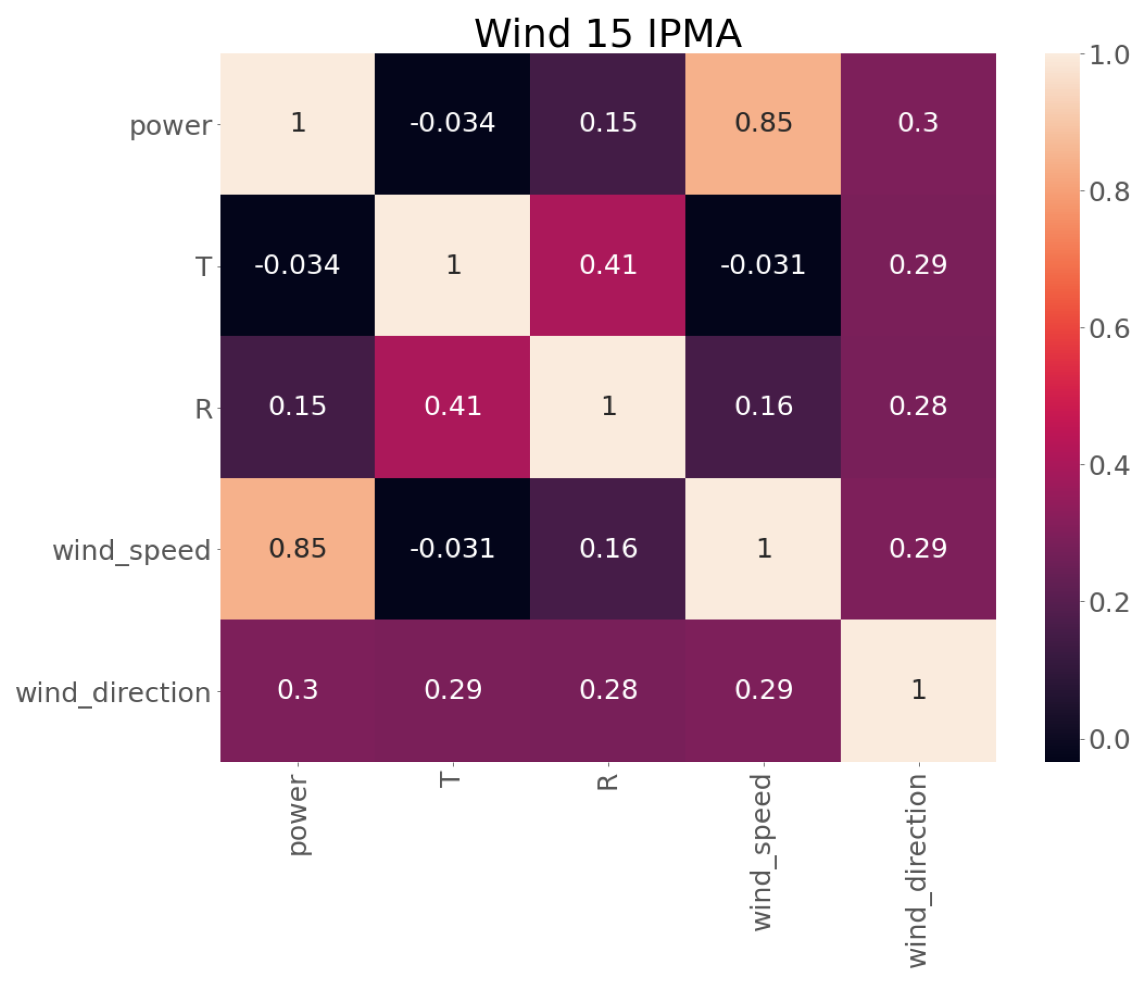
To select the appropriate features, a correlation matrix, which provides the relationship between variables, is used. The correlation coefficients can fall between −1 and +1, where a high and positive correlation indicates that the variables measured using the same characteristic. Thus, the features with the higher correlation with the target variable (power) are chosen, and the features with negative or low correlation are discarded. Figure 2 presents the correlation matrix of wind farm 15.
Based on the correlation matrix, only the wind speed and wind direction features are selected to forecast the power generation. Wind speed presents a higher correlation, as expected, followed by wind direction, which, despite not having a very high correlation, may be relevant. The other variables, temperature and solar radiance, are discarded because they have either a negative or a very low correlation.
2.4. Forecasting Models
Once the outliers are removed, the missing values are filled or handled, and the feature selection has been performed, the final dataset is divided into the following two subsets:
- Training set, the data used by the model to discover and to learn patterns between the features and the forecast variable, power.
- Test set, the data on which the power predictions are generated. It corresponds to unseen data used to evaluate the performance of the model.
The training set is normally larger than the test set because the idea is to feed the model with as much data as possible, to learn meaningful patterns, and then apply the things learned to create predictions on unseen data.
In this case, eight different forecasting models are implemented to predict the power generation of the 20 wind farms, starting from persistence (to have a benchmark), passing through regressive models, a neural network, and some newer models.
Specifically, the following forecasting models are tested:
2.4.1. Persistence
The persistence forecast in this case corresponds to the power measured at the same time instant from the previous day, or at 96-time intervals before the desired forecast time instant, considering a data resolution of 15 min. It can be formulated as:
where is the wind power forecast value at a certain instant of time, and is the wind power value measured 96 time intervals beforehand.
2.4.2. Auto-Regressive (AR)
This model uses observations from previous time steps as input for the regression equation, to predict the value at the next time step. In simple terms, an AR(p) model relates p past observations to the current value as [25]:
where is the mean value, is a coefficient which reflects each past observation’s influence on the current value, and is the actual stochastic perturbation.
2.4.3. Auto-Regressive with Exogenous Variable (ARX)
AN ARX model is an auto-regressive model with exogenous inputs. It assumes a stationary and invertible process, where the exogenous inputs come from an external system. Therefore, an ARX(p, ) model can described as [26]:
where is the exogenous coefficient and is the order of the exogenous inputs.
2.4.4. Long Short-Term Memory (LSTM) Neural Network
LSTM is one of many types of RNN. Since RNNs cannot store long-time memory, LSTMs proved to be very useful in forecasting with long-time data, based on ’memory line’. In an LSTM, the memorization of earlier stages is performed through gates. In the end, the sigmoidal neural network layer composing the gates drives the cell to an optimal value by disposing of or letting data pass through. Each sigmoid layer has a binary value (0 or 1), with 0 meaning to let nothing pass through, and 1 meaning to let everything pass through. Figure 3 shows the composition of the LSTM nodes [27].
To develop the LSTM neural network model in Python, the library tensorflow.keras-.layers.LSTM was used.
2.4.5. Decision Trees (DTs)
DTs are a common way of representing the decision-making process through a branching, tree-like structure. They are made up of different nodes, where the root node is the start of the decision tree, which is usually the whole dataset. Leaf nodes are the endpoint of a branch or the final output of a series of decisions. The features of the data are internal nodes, and the outcome is the leaf node [28]. Figure 4 presents the basic structure of a decision tree.
To develop the DT model in Python, the library sklearn.tree.DecisionTreeRegressor was used.
2.4.6. Random Forest (RF)
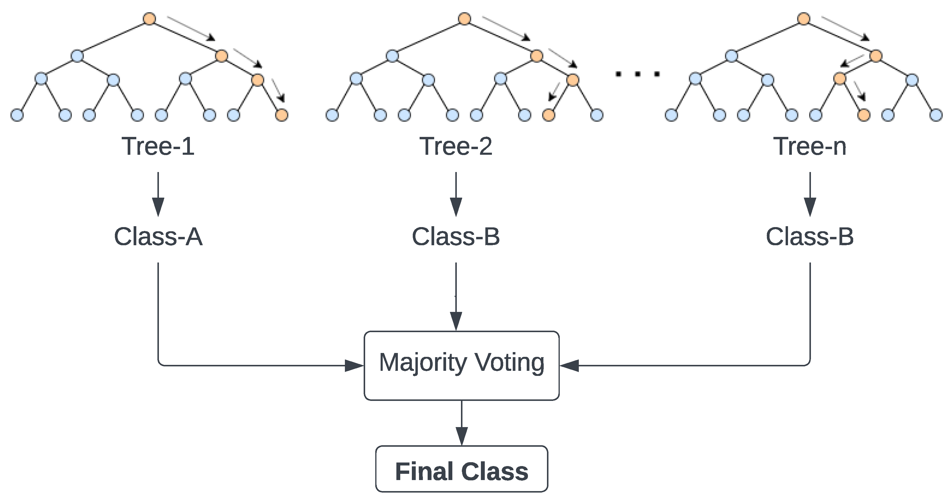
RF is a method that combines several decision trees and that uses the majority voting of the individual trees to find the overall class. It consists of three steps: randomly selecting training data when making trees, choosing some subsets of features when splitting nodes, and employing only a subset of all features for splitting each node in each simple decision tree. During the training of the data, each tree learns from a random sample of the data points [30]. Figure 5 shows the composition of the ’n’ number of trees, which constructs the RF algorithm.
To develop the RF model in Python, the library sklearn.ensemble.RandomForest- Regressor was used.
2.4.7. Extreme Gradient Boosting (XGBOOST)
XGBOOST is one of the most efficient implementations of gradient-boosted decision trees, specifically designed to optimize memory usage and to exploit the hardware computing power. The main idea of boosting is to sequentially build subtrees from an original tree, such that each subsequent tree reduces the errors of the previous one. In such a way, the new subtrees will update the previous residuals in order to reduce the error of the cost function. The process of additive learning in XGBOOST, as explained by N.Dhieb et al. [32], is presented below.
First, consider a data set D, expressed as follows:
where m is the dimension of the features , is the response of the sample i, and n is the number of samples. The vertical bars in Equation (5) denote the cardinality of the set.
Then, the predicted value of the entry i and denoted as , is defined as:
where indicates an independent tree in the space of the regression trees. F and refer to the predicted score given by the i-th sample and k-th tree.
The objective function of the XGBOOST, denoted by , is given as follows:
By minimizing the objective function , the regression tree model functions can be learned. The training loss function evaluates the difference between the prediction and the actual value . Herein, the term is used to avoid the overfitting problem by penalizing the model complexity as follows:
where and are regularization parameters. T and w are, respectively, the numbers of leaves and the scores on each leaf.
A second-degree Taylor series can be used to approximate the objective function. Let’s define , an instance set of leaf j with , a fixed structure. The optimal weights of leaf j and the corresponding optimal value can be obtained using the following equations:
where and are the first and the second gradient orders of the loss function . The loss function can be used as a quality score of the tree structure q. The smaller the score is, the better the model is.
As it is not possible to enumerate all of the tree structures, a greedy algorithm can solve the problem by starting from a single leaf and by iteratively adding branches to the tree. Let’s say that and are the instance sets of the right and left nodes after the split. Assuming , the loss reduction after the split is given as:
This formula is usually used in practice for evaluating the split candidates. The XGBOOST model uses many simple trees and score leaf nodes during splitting. The first three terms of the equation represent, respectively, the scores of the left, right, and original leaf. In addition, the term is the regularization on the additional leaf and it will be used in the training process.
To develop the XGBOOST model in Python, the library xgboost.XGBRegressor was used.
2.4.8. Support Vector Machine (SVM)
SVM regression trains the model using a symmetrical loss function, which penalizes for both high and low misestimates. The aim is to find a hyperplane that differentiates the data points plotted in multi-dimensional space, where each dimension represents the different features used.
The hyperplane having a maximum separation distance is used to meet the request of the regression with a higher degree of accuracy. Different coordinates on the plot are obtained by mapping the parameters under observation on the plot. It can be described with the help of the mapping function formulated as [29]:
where is the weighted vector and is the mapped regressor.
To develop the SVM model in Python, the library sklearn.svm.SVR was used.
2.5. Post-Processing
The main purpose of this stage is to check the generated power predictions and to adjust the values out of range if they exist. To achieve that, the algorithm checks two conditions:
- . The predicted power cannot be negative. In the case where there are negative values, they are adjusted to 0.
- . The predicted power cannot be higher than the installed capacity of the wind farm. In this case, the maximum forecast value is limited to the installed capacity.
Once both conditions are verified or adjusted if necessary, the final wind power predictions are saved, and a plot comparing the forecast values with the real values is generated. An example of this plot is presented in Figure 6, where the XGBOOST method is used to forecast 1 month of 2020 (JUL), by using 6 months of training (January–June of 2020). In the figure, it is possible to see that the forecast method arrives at predicting the trends of the wind generation, but it presents a higher error when the production is high during short periods of time.
2.6. Validation
The error metric defined to evaluate the performance of the forecasting models is based on the Root Mean Square Error (RMSE), but with a small difference: in this case, the RMSE is normalized by dividing by the installed capacity of the wind farm. Hence, it is called the Relative Root Mean Square Error (RRMSE) and it is calculated as:
where N is the total number of samples, is the forecast value, is the measured value, and is the installed capacity of the wind farm.
Basically, the algorithm calculates the daily RRMSE between the predictions and the real values for the test period defined, and then the average of this daily error is reported (as a percentage), to have an idea of the accuracy of the forecast made. This RRMSE metric is used as a comparison point in all the results presented.
3. Results and Discussion
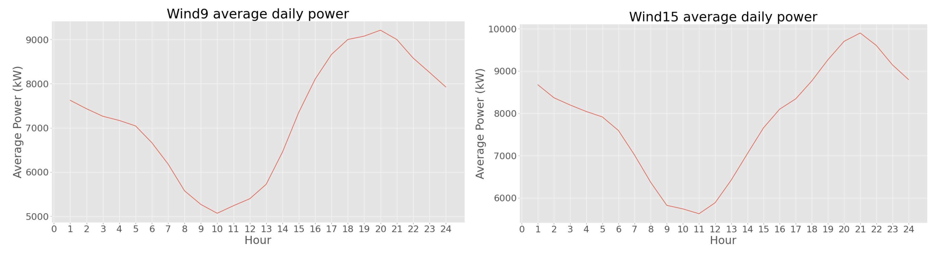
This section presents the results obtained for the forecasting models developed, the comparison of the RRMSE between them, and the DSO results. It also presents the different tests and the tuning process performed to the best-suited model in order to improve the results. The wind farms’ installed power range from 2 MW to 45 MW. As an example, the average production behavior of two wind farms is presented in Figure 7.
3.1. WPGF Models
Table 2 presents the RRMSE for the Persistence, AR, and ARX models; Table 3 presents the RRMSE for the LSTM, DT, RF, XGBOOST, and SVM models. The training and test periods defined in all the simulations correspond to: June–November of 2021 for training, and December of 2021 for forecast. The meteorological parameters, wind speed and wind direction, were used as features in the models that use exogenous variables, as determined in Section 2.3.
The results obtained in Table 2 and Table 3 show that just three methods, ARX (21.046%), RF (20.354%), and XGBOOST (18.613%) outperformed the DSO results (22.904%). Since XGBOOST has a lower RRMSE, it is chosen as the method to be focused upon and to be improved, in order to reduce the percentage of error even more.
At this point, the main objective of this work has been achieved, considering that the developed and implemented XGBOOST model can forecast wind power generation with a higher accuracy than the model currently used by the DSO. In addition, the computation time, which is also a determinant factor for the DSO, is on average between 20–30 s per wind farm for the XGBOOST model, which is highly efficient.
Now, some tests and improvements to the XGBOOST algorithm are developed and executed, with the idea of improving the results as much as possible.
3.2. XGBOOST, Adjusting Training, and Test Periods
The first test consists of adjusting the training and test periods, to compare the RRMSE of the XGBOOST model under different time horizons. Based on the two years of IPMA data available (2020 and 2021), the following eight combinations of training and test periods are defined:
- Combination 1: 6 months training (January–June of 2021) and 6 months forecast (July–December of 2021).
- Combination 2: 7 months training (January–July of 2021) and 5 months forecast (August–December of 2021).
- Combination 3: 8 months training (January–August of 2021) and 4 months forecast (September–December of 2021).
- Combination 4: 9 months training (January–September of 2021) and 3 months forecast (October–December of 2021).
- Combination 5: 10 months training (January–October of 2021) and 2 months forecast (November–December of 2021).
- Combination 6: 11 months training (January–November of 2021) and 1 month forecast (December of 2021).
- Combination 7: 1 year training (January–December of 2020) and 6 months forecast (January–June of 2021).
- Combination 8: 1 year training (January–December of 2020) and 1 year forecast (January–December of 2021).
The results obtained are summarized in Figure 8, which presents the average RRMSE of the 20 wind farms for each combination, achieved by the XGBOOST model and by the model used by the DSO. To have a fair comparison between the different combinations, regardless of the number of months to forecast, the RRMSE of the same month (DEC of 2021) was analyzed independently of the combination.
Figure 8 shows that first, the error of the XGBOOST model developed is always lower than the error of the DSO for any combination of training and test sets. Second, the XGBOOST model more accurately forecasts long periods of time, such as 6 months (Combination 7) or 1 complete year (Combination 8), instead of short periods of time such as 1 month (Combination 6) or 2 months (Combination 5). Third, the best combination found corresponds to Combination number 7: 1-year training (January–December of 2020) and 6 months forecast (January–June of 2021), with an average RRMSE of 14.257%. From now on, these training and forecast periods are used in all tests.
3.3. XGBOOST Hyperparameter Tuning
Hyperparameter tuning or hyperparameter optimization is the process of determining the right combination of hyperparameters that maximizes an ML or AI model performance. It works by running multiple trials of different combinations of hyperparameters in a single training process. Once the process ends, it gives the set of hyperparameter values that are best suited for the model to give the most optimal result [33]. The hyperparameters of XGBOOST that are tuned are the following [34]:
- max depth: Maximum depth per tree. A deeper tree might increase the performance, but also the complexity and the chances to overfit. The value must be an integer greater than 0. The default is 6.
- learning rate: Determines the step size at each iteration while the model optimizes toward its objective. A low learning rate makes computation slower and requires more rounds to achieve the same reduction in residual error as a model with a high learning rate. The value must be between 0 and 1. The default is 0.3.
- n estimators: The number of trees in our ensemble. Equivalent to the number of boosting rounds. The value must be an integer that is greater than 0. The default is 100.
- colsample bytree: Represents the fraction of columns to be randomly sampled for each tree. It might improve overfitting. The value must be between 0 and 1. The default is 1.
- sub-sample: Represents the fraction of observations to be sampled for each tree. Lower values prevent overfitting but might lead to underfitting. The value must be between 0 and 1. The default is 1.
- min child weight: Defines the minimum sum of weights of all observations required in a child. It is used to control overfitting. The larger it is, the more conservative the algorithm will be. The value must be an integer greater than 0. The default is 1.
To find the best combination of hyperparameters for the XGBOOST model, a Random Search optimization algorithm is used. It consists of a large range of hyperparameter values, which are randomly iterated a specific number of times over the combinations of the values defined. The number of iterations defined for the Random Search is 50, and the Mean Square Error (MSE) is the metric used to evaluate the performance for each combination of hyperparameters. This process is performed only once because the computation time is very high and it takes a long time to obtain the results.
Table 4 presents the best combination of hyperparameters obtained for each wind farm after running Random Search and the average values of each hyperparameter when considering the 20 wind farms altogether.
Considering the values in Table 4, two tests, one using the best combination of hyperparameters for each wind farm (Best combination) and the other using the same average values of hyperparameters for all wind farms (Average values) are performed. The idea is to compare the best RRMSE achieved so far (Best results until now), with the RRMSE obtained after the hyperparameter optimization. The results are presented in Table 5, using 1-year training (January–December of 2020) and 6 months forecast (January–June of 2021) that was the best combination found in Section 3.2.
From Table 5, it is possible to observe that the average RRMSE was reduced from 14.257% to 13.180% after the hyperparameter tuning was performed specifically for each wind farm, meaning there was an improvement of 7.55%. In the other case, where the RRMSE was computed using the average values of hyperparameters instead of the specific combination found for every wind farm, the average RRMSE achieved was 13.481%. In both cases, a considerable reduction in the error was achieved with the hyperparameter tuning.
After the comparison between the two tests performed, it was decided that for future forecasts, just the average combination of hyperparameters (max depth = 2, learning rate = 0.04, nestimators = 343, colsample bytree = 0.9, subsample = 0.8, min child weight = 7) will be used to run the XGBOOST model independently of the wind farm. This considered that the DSO has 200 wind farms connected to the MV distribution network of Portugal, and that running Random Search for each one is not worth the computation time required (around 12 h per wind farm) for the little extra improvement obtained when calculating the best combination of hyperparameters specific for every wind farm.
3.4. XGBOOST with Backtesting
Backtesting is a term used in modeling that refers to the testing of a predictive model on historical data. It involves moving backwards in time, step by step, in as many stages as it is necessary. Hence, it is a special type of cross-validation applied to previous periods [35].
The purpose of this test is then to apply the backtesting with refit, and increasing training size strategy inside the XGBOOST model, to see if the RRMSE can be reduced. To achieve that, the model is trained each time before making a new prediction, and then that prediction is included in the training set and the process is repeated until all the predictions are made. That means that the model uses all the data available so far, while the training set increases sequentially, maintaining the temporal order of the data.
The initial training set in our case corresponds to 1 year of data (January–December of 2020), the prediction horizon corresponds to 1 day (meaning that the model is trained in each iteration to forecast each day separately) and the retraining is performed until the 6 months (January–June of 2021), that correspond to the forecast period is predicted.
Table 6 presents the RRMSE achieved when using the backtesting strategy implemented inside the XGBOOST model.
As shown in Table 6, the results obtained with backtesting are better than the best RRMSE achieved until now. There is a little improvement of 2.8% since the error was reduced from 13.481% to 13.097%. However, when considering the computation time that backtesting requires, which is on average 10 h per wind farm, the small reduction in the error makes it not worth implementing this strategy inside the model.
For the DSO, it is important that the model is able to perform the forecast in a short computing time because they have 200 wind farms connected to the MV distribution network of Portugal. The implemented XGBOOST model takes between 20–30 s per wind farm to run, and with backtesting, it takes 1500 times more. Since the accuracy of the forecast with backtesting does not represent a significant improvement when compared with the normal XGBOOST, the inclusion of backtesting is discarded.
3.5. Stacking
Stacking is the process of using different machine learning and AI models one after another, where the predictions from each model are added as new features. It is performed in layers, and there can be arbitrarily many layers, dependent on exactly how many models are trained, along with the best combinations of these models. In the end, the final dataset combines the initial features plus the predictions created after each layer is fed into the last model. The last model is called a meta-learner, and its purpose is to generalize all the features from each layer into the final predictions [36].
Figure 9 presents the diagram of the stacking process implemented in this case.
First, six layers were defined using the following models: RF, Light Gradient Boosting Machine (LGBM), XGBOOST, Ridge, Lasso, and SVM. Then, the XGBOOST model was used again as a meta-learner to obtain the final predictions.
Table 7 presents the RRMSE obtained using the stacking approach, with the RF, LGBM, XGBOOST, Ridge, Lasso, and SVM layers; and the XGBOOST meta-learner, for 1-year training and 6 months forecast.
As shown in Table 7, by stacking the RRMSE passed from 13.481% to 13.392%, this is equivalent a 0.66% improvement. Regarding the computation time required by this approach, for each wind farm, it takes on average 15 min to run, which is 40 times more than the normal XGBOOST (that takes between 20–30 s to run). Therefore, even when the RRMSE results are better when using stacking, the little reduction in the error is not worth the extra computation time, and stacking is discarded.
4. Conclusions
In this paper, eight different forecasting models, namely, Persistence, AR, ARX, LSTM neural network, DT, RF, XGBOOST, and SVM were developed and tested to predict the power generation of 20 wind farms connected to the secondary substations of the MV distribution network of Portugal. This value is considered as representative of the total number of wind farms at the distribution level. After comparing the models between them and with the DSO predictions, the results showed that for 6 months of training (June–November of 2021) and 1-month forecast (December of 2021), XGBOOST obtained the best performance, with an RRMSE of 18.613%, followed by RF with an RRMSE of 20.354% and ARX with an RRMSE of 21.046%. The rest of the models obtained an error that is higher than the error of the DSO predictions for the same period, which corresponds to an RRMSE of 22.904%. Specifically, the LSTM neural network, DT, AR, SVM, and Persistence obtained, respectively, RRMSEs of 24.160%, 24.381%, 27.522%, 29.822%, and 31.838%. Another aspect as important as the accuracy itself is the computation time, and in this study, the computation time required to run any of the models is less than one minute, which can be considered as computationally efficient.
With XGBOOST as the best-suited forecasting model for the wind farms analyzed, some tests and improvements were performed on this method in order to reduce the error as much as possible. It was found that the best combination of training and test periods based on the two years of information available for IPMA, corresponds to 1 year of training (January–December of 2020) and 6 months of forecast (January–June of 2021). When using this specific combination, the average RRMSE is reduced to 14.257%.
A hyperparameter tuning of XGBOOST using Random Search optimization was carried out to improve the previous result. The best combination of hyperparameters was found for each wind farm and the average RRMSE was reduced to 13.180%. However, since the computation time to run Random Search (around 12 h) is very high, it was decided to use the average values of the hyperparameters independently of the wind farm. Using the average values of the hyperparameters, the RRMSE achieved is 13.481%, which is not so far from the value obtained using the best combination of hyperparameters, and therefore, this approach should be used for future forecasts or with new wind farms.
Other improvements that lowered the best RRMSE (13.481%) of the developed XGBOOST model were achieved using backtesting and stacking approaches. In the case of backtesting, the RRMSE was reduced to 13.097%, while for stacking, the RRMSE was reduced to 13.392%. Nevertheless, both processes require a longer computation time, 10 h per wind farm for backtesting and 15 min per wind farm for stacking, than the normal XGBOOST model, which takes only between 20 to 30 s per wind farm to run. Since one of the most important characteristics of a forecasting model is to make predictions in an efficient way, meaning rapidly and with accuracy, it was concluded that the small reduction in the error achieved with this strategy is not worth the large computation time needed, and consequently, backtesting and stacking are discarded.
After all, using the proposed XGBOOST model for 1 year of training (January–December of 2020) and 6 months forecast (January–June of 2021), the best average RRMSE achieved for the 20 wind farms studied corresponds to 13.481%—after discarding Random Search, backtesting, and stacking, of course. The results successfully fulfilled the main objective of this work, which was to improve the performance of the actual DSO forecasting system, which for the same period of analysis, presents an RRMSE of 16.827%. With the XGBOOST model developed, an improvement of 20% is achieved. The framework is scalable, computationally efficient, and can be used for future wind power forecasting if the DSO wants to obtain predictions with higher accuracy.
In future work, it is expected that methods will be developed that allow for the probabilistic forecast of wind generation. The methods will be also tested in other sources of generation such as solar photovoltaic. Afterwards, the impacts of the proposed forecast methods on the operational planning tools will be assessed.
Author Contributions
Conceptualization, H.A., P.M.S.C. and H.M.; methodology, H.A. and H.M.; software, H.A.; validation, P.M.S.C. and H.M.; formal analysis, H.M.; investigation, H.A. and H.M.; resources, P.M.S.C. and H.M.; data curation, H.A.; writing—original draft preparation, H.A.; writing—review and editing, P.M.S.C. and H.M.; supervision, P.M.S.C. and H.M.; project administration, P.M.S.C. and H.M.; funding acquisition, P.M.S.C. All authors have read and agreed to the published version of the manuscript.
Funding
This work was partially supported by Portuguese national funds through Fundação para a Ciência e a Tecnologia with reference UIDB/50021/2020, and by the European Union’s Horizon Europe research and innovation programme under grant agreement No. 10105676. This work also had the support of E-REDES, the Distribution System Operator on the Portuguese mainland.
Conflicts of Interest
The authors declare no conflict of interest.
Nomenclature
| ANFIS | Adaptative Neural Fuzzy Inference System |
| ANNs | Artificial Neural Networks |
| AR | Auto-Regressive |
| ARX | Auto-Regressive with Exogenous Variable |
| ARIMA | Auto-Regressive Integrated Moving Average |
| ARMA | Auto-Regressive Moving Average |
| BPNN | Back-Propagation Neural Network |
| DSO | Distribution System Operator |
| DTs | Decision Trees |
| EDA | Exploratory Data Analysis |
| EU | European Union |
| FFNN | Feed Forward Neural Network |
| IPMA | Instituto Português do Mar e da Atmosfera |
| LGBM | Light Gradient Boosting Machine |
| LSTM | Long Short-Term Memory |
| MAPE | Mean Absolute Percentage Error |
| ML | Machine Learning |
| MV | Medium Voltage |
| NWP | Numerical Weather Prediction |
| PV | Solar Photovoltaic |
| RESs | Renewable Energy Sources |
| RF | Random Forest |
| RMSE | Root Mean Square Error |
| RNN | Recurrent Neural Network |
| RRMSE | Relative Root Mean Square Error |
| SVM | Support Vector Machine |
| TSO | Transmission System Operator |
| WEPs | Weather Ensemble Predictions |
| WPGF | Wind Power Generation Forecast |
| XGBOOST | Extreme Gradient Boosting |
References
- Micheli, S. Policy Strategy Cooperation in the 2030 Climate and Energy Policy Framework. Atl. Econ. J. 2020, 48, 265–267. [Google Scholar] [CrossRef]
- Javed, M.S.; Ma, T.; Jurasz, J.; Amin, M.Y. Solar and wind power generation systems with pumped hydro storage: Review and future perspectives. Renew. Energy 2020, 148, 176–192. [Google Scholar] [CrossRef]
- GWEC Global Wind Energy Council. Available online: https://gwec.net/global-wind-report-2021/ (accessed on 24 April 2022).
- Taylor, J.W.; McSharry, P.E.; Buizza, R. Wind power density forecasting using ensemble predictions and time series models. IEEE Trans. Energy Convers. 2009, 24, 775–782. [Google Scholar] [CrossRef]
- Machado, E.P.; Morais, H.; Pinto, T. Wind Speed Forecasting Using Feed-Forward Artificial Neural Network. In Distributed Computing and Artificial Intelligence, Proceedings of the 18th International Conference, DCAI 2021, Salamanca, Spain, 6–8 October 2021; Lecture Notes in Networks and Systems; Matsui, K., Omatu, S., Yigitcanlar, T., González, S.R., Eds.; Springer: Cham, Stwitzerland, 2022; Volume 327. [Google Scholar] [CrossRef]
- Sijakovic, N.; Terzic, A.; Fotis, G.; Mentis, I.; Zafeiropoulou, M.; Maris, T.I.; Zoulias, E.; Elias, C.; Ristic, V.; Vita, V. Active System Management Approach for Flexibility Services to the Greek Transmission and Distribution System. Energies 2022, 15, 6134. [Google Scholar] [CrossRef]
- Zafeiropoulou, M.; Mentis, I.; Sijakovic, N.; Terzic, A.; Fotis, G.; Maris, T.I.; Vita, V.; Zoulias, E.; Ristic, V.; Ekonomou, L. Forecasting Transmission and Distribution System Flexibility Needs for Severe Weather Condition Resilience and Outage Management. Appl. Sci. 2022, 12, 7334. [Google Scholar] [CrossRef]
- Wilczek, P. Connecting the dots: Distribution grid investments to power the energy transition. In Proceedings of the 11th Solar & Storage Power System Integration Workshop (SIW 2021), Online, 28 September 2021; Volume 2021, pp. 1–18. [Google Scholar] [CrossRef]
- Vargas, S.A.; Esteves, G.R.T.; Maçaira, P.M.; Bastos, B.Q.; Oliveira, F.L.C.; Souza, R.C. Wind power generation: A review and a research agenda. J. Clean. Prod. 2019, 218, 850–870. [Google Scholar] [CrossRef]
- Ernst, B.; Oakleaf, B.; Ahlstrom, M.L.; Lange, M.; Moehrlen, C.; Lange, B.; Focken, U.; Rohrig, K. Predicting the wind. IEEE Power Energy Mag. 2007, 5, 78–89. [Google Scholar] [CrossRef]
- Soman, S.S.; Zareipour, H.; Malik, O.; Mandal, P. A review of wind power and wind speed forecasting methods with different time horizons. In Proceedings of the IEEE North American Power Symposium, Arlington, TX, USA, 26–28 September 2010; pp. 1–8. [Google Scholar] [CrossRef]
- Wu, Y.K.; Hong, J.S. A literature review of wind forecasting technology in the world. In Proceedings of the 2007 IEEE Lausanne Powertech, Lausanne, Switzerland, 1–5 July 2007; pp. 504–509. [Google Scholar] [CrossRef]
- Gallego, C.; Pinson, P.; Madsen, H.; Costa, A.; Cuerva, A. Influence of local wind speed and direction on wind power dynamics—Application to offshore very short-term forecasting. Appl. Energy 2011, 88, 4087–4096. [Google Scholar] [CrossRef] [Green Version]
- Duran, M.J.; Cros, D.; Riquelme, J. Short-term wind power forecast based on ARX models. J. Energy Eng. 2007, 133, 172–180. [Google Scholar] [CrossRef]
- Machado, E.; Pinto, T.; Guedes, V.; Morais, H. Electrical Load Demand Forecasting Using Feed-Forward Neural Networks. Energies 2021, 14, 7644. [Google Scholar] [CrossRef]
- Catalão, J.D.S.; Pousinho, H.M.I.; Mendes, V.M.F. Short-term wind power forecasting in Portugal by neural networks and wavelet transform. Renew. Energy 2011, 36, 1245–1251. [Google Scholar] [CrossRef]
- Mabel, M.C.; Fernandez, E. Analysis of wind power generation and prediction using ANN: A case study. Renew. Energy 2008, 33, 986–992. [Google Scholar] [CrossRef]
- Hanifi, S.; Liu, X.; Lin, Z.; Lotfian, S. A critical review of wind power forecasting methods—Past, present and future. Energies 2020, 13, 3764. [Google Scholar] [CrossRef]
- Jung, J.; Broadwater, R.P. Current status and future advances for wind speed and power forecasting. Renew. Sustain. Energy Rev. 2014, 31, 762–777. [Google Scholar] [CrossRef]
- Khazaei, S.; Ehsan, M.; Soleymani, S.; Mohammadnezhad-Shourkaei, H. A high-accuracy hybrid method for short-term wind power forecasting. Energy 2022, 238, 122020. [Google Scholar] [CrossRef]
- Zheng, H.; Wu, Y. A xgboost model with weather similarity analysis and feature engineering for short-term wind power forecasting. Appl. Sci. 2019, 9, 3019. [Google Scholar] [CrossRef] [Green Version]
- Kassa, Y.; Zhang, J.H.; Zheng, D.H.; Wei, D. Short term wind power prediction using ANFIS. In Proceedings of the 2016 IEEE International Conference On Power And Renewable Energy (ICPRE), Shanghai, China, 21–23 October 2016; pp. 338–393. [Google Scholar] [CrossRef]
- Fugon, L.; Juban, J.; Kariniotakis, G. Data mining for wind power forecasting. In Proceedings of the 2008 European Wind Energy Conference & Exhibition (EWEC), Brussels, Belgium, 31 March–3 April 2008; Available online: https://hal-mines-paristech.archives-ouvertes.fr/hal-00506101 (accessed on 16 February 2023).
- Feature Selection Techniques in Machine Learning. Available online: https://www.javatpoint.com/feature-selection-techniques-in-machine-learning (accessed on 18 May 2022).
- Santamaría-Bonfil, G.; Reyes-Ballesteros, A.; Gershenson, C. Wind speed forecasting for wind farms: A method based on support vector regression. Renew. Energy 2016, 85, 790–809. [Google Scholar] [CrossRef]
- Akouemo, H.N.; Povinelli, R.J. Data improving in time series using ARX and ANN models. IEEE Trans. Power Syst. 2017, 32, 3352–3359. [Google Scholar] [CrossRef] [Green Version]
- Moghar, A.; Hamiche, M. Stock market prediction using LSTM recurrent neural network. Procedia Comput. Sci. 2020, 170, 1168–1173. [Google Scholar] [CrossRef]
- Decision Trees in Machine Learning Explained. Available online: https://www.seldon.io/decision-trees-in-machine-learning (accessed on 25 May 2022).
- Chaudhary, A.; Sharma, A.; Kumar, A.; Dikshit, K.; Kumar, N. Short term wind power forecasting using machine learning techniques. J. Stat. Manag. Syst. 2020, 23, 145–156. [Google Scholar] [CrossRef]
- Ahmadi, A.; Nabipour, M.; Mohammadi-Ivatloo, B.; Amani, A.M.; Rho, S.; Piran, M.J. Long-term wind power forecasting using tree-based learning algorithms. IEEE Access 2020, 8, 151511–151522. [Google Scholar] [CrossRef]
- Jørgensen, K.L.; Shaker, H.R. Wind power forecasting using machine learning: State of the art, trends and challenges. In Proceedings of the 2020 IEEE 8th International Conference on Smart Energy Grid Engineering (SEGE), Oshawa, ON, Canada, 12–14 August 2020; pp. 44–50. [Google Scholar] [CrossRef]
- Dhieb, N.; Ghazzai, H.; Besbes, H.; Massoud, Y. Extreme gradient boosting machine learning algorithm for safe auto insurance operations. In Proceedings of the 2019 IEEE International Conference on Vehicular Electronics and Safety (ICVES), Cairo, Egypt, 4–6 September 2019; pp. 1–5. [Google Scholar] [CrossRef]
- Hyperparameter Tuning in Python: A Complete Guide. Available online: https://neptune.ai/blog/hyperparameter-tuning-in-python-complete-guide (accessed on 5 June 2022).
- XGBoost: A Complete Guide to Fine-Tune and Optimize Your Model. Available online: https://towardsdatascience.com/xgboost-fine-tune-and-optimize-your-model-23d996fab663 (accessed on 7 June 2022).
- Skforecast: Time Series Forecasting with Python and Scikit-Learn. Available online: https://www.cienciadedatos.net/documentos/py27-time-series-forecasting-python-scikitlearn.html (accessed on 3 August 2022).
- Stack Machine Learning Models—Get Better Results. Available online: https://mlfromscratch.com/model-stacking-explained/ (accessed on 20 August 2022).
Figure 1.
Methodology stages.

Figure 2.
Correlation matrix of wind farm 15.

Figure 3.
Every LSTM node consists of a set of cells responsible for storing passed data streams. The upper line in each cell links the models as a transport line, handing over data from the past to the present ones, and the independence of cells helps the model to filter aggregate values from one cell to another [27].

Figure 4.
DT structure [29].
Figure 4.
DT structure [29].

Figure 5.
Composition of RF [31].
Figure 5.
Composition of RF [31].

Figure 6.
Forecast vs. real values plot for 6 months training, 1-month forecast using XGBOOST.

Figure 7.
Average production of wind farm 9 (left) and wind farm 15 (right).

Figure 8.
Average RRMSE for each combination.

Figure 9.
Stacking process implemented [36].
Figure 9.
Stacking process implemented [36].


Table 1.
Descriptive statistics of wind farm 15.
| Measure | Power (kW) | T (K) | R (W/m2) | Wind Speed (m/s) | Wind Direction () |
|---|---|---|---|---|---|
| Mean | 7834.07 | 288.58 | 735.84 | 7.01 | 241.51 |
| Std Dev | 7177.94 | 4.95 | 729.82 | 2.80 | 109.90 |
| Min | 0.00 | 272.94 | 0.00 | 0.14 | 0.02 |
| 25th Perc | 1600.00 | 285.25 | 86.43 | 4.93 | 157.24 |
| 50th Perc | 5610.00 | 288.11 | 524.35 | 6.92 | 284.33 |
| 75th Perc | 13,102.50 | 291.45 | 1193.59 | 9.08 | 338.96 |
| Max | 29,705.29 | 310.58 | 2814.88 | 16.32 | 359.98 |
Table 2.
RRMSE for Persistence, AR, and ARX: 6 months training, 1-month forecast.
| Wind Farm | Persistence (%) | AR (%) | ARX (%) | DSO (%) |
|---|---|---|---|---|
| 1 | 24.594 | 16.886 | 15.384 | 13.482 |
| 2 | 37.717 | 35.105 | 19.248 | 16.187 |
| 3 | 14.895 | 12.396 | 12.515 | 41.013 |
| 4 | 35.714 | 32.035 | 28.131 | 19.850 |
| 5 | 30.814 | 26.713 | 20.364 | 14.874 |
| 6 | 32.897 | 27.102 | 21.185 | 18.929 |
| 7 | 35.403 | 28.947 | 19.673 | 50.877 |
| 8 | 38.103 | 32.230 | 27.287 | 21.536 |
| 9 | 30.248 | 26.306 | 20.168 | 14.372 |
| 10 | 34.136 | 30.781 | 20.690 | 45.416 |
| 11 | 31.939 | 29.759 | 23.380 | 29.586 |
| 12 | 24.222 | 19.232 | 17.073 | 15.593 |
| 13 | 33.787 | 29.940 | 18.394 | 17.470 |
| 14 | 38.087 | 30.688 | 25.111 | 21.550 |
| 15 | 26.191 | 20.947 | 13.660 | 11.954 |
| 16 | 37.940 | 26.028 | 36.241 | 21.983 |
| 17 | 34.902 | 23.803 | 29.912 | 19.541 |
| 18 | 34.712 | 28.478 | 33.975 | 26.619 |
| 19 | 31.060 | 19.225 | 24.680 | 18.242 |
| 20 | 29.404 | 21.114 | 26.565 | 18.998 |
| Average | 31.838 | 27.522 | 21.046 | 22.904 |
Table 3.
RRMSE for LSTM, DT, RF, XGBOOST, and SVM: 6 months training, 1-month forecast.
| Wind Farm | LSTM (%) | DT (%) | RF (%) | XGBOOST (%) | SVM (%) | DSO (%) |
|---|---|---|---|---|---|---|
| 1 | 23.209 | 19.543 | 12.371 | 12.451 | 19.492 | 13.482 |
| 2 | 24.413 | 24.596 | 19.952 | 17.637 | 31.561 | 16.187 |
| 3 | 8.288 | 15.671 | 11.257 | 10.549 | 10.399 | 41.013 |
| 4 | 29.888 | 28.721 | 28.698 | 22.649 | 47.410 | 19.850 |
| 5 | 22.727 | 21.783 | 14.873 | 13.617 | 29.755 | 14.874 |
| 6 | 22.555 | 25.147 | 23.205 | 19.273 | 35.377 | 18.929 |
| 7 | 29.426 | 32.046 | 21.851 | 21.101 | 20.949 | 50.877 |
| 8 | 25.833 | 25.484 | 25.398 | 24.427 | 39.240 | 21.536 |
| 9 | 26.900 | 23.291 | 17.296 | 17.472 | 24.699 | 14.372 |
| 10 | 26.700 | 22.602 | 21.286 | 16.374 | 28.953 | 45.416 |
| 11 | 21.877 | 25.785 | 22.783 | 21.412 | 34.463 | 29.586 |
| 12 | 19.562 | 23.656 | 17.673 | 17.509 | 23.907 | 15.593 |
| 13 | 21.859 | 17.593 | 18.195 | 12.947 | 26.973 | 17.470 |
| 14 | 26.925 | 29.963 | 26.919 | 28.127 | 36.026 | 21.550 |
| 15 | 22.833 | 17.059 | 12.828 | 11.651 | 15.297 | 11.954 |
| 16 | 29.310 | 25.150 | 22.071 | 20.628 | 37.585 | 21.983 |
| 17 | 27.285 | 26.611 | 25.206 | 21.862 | 45.642 | 19.541 |
| 18 | 24.323 | 31.979 | 28.080 | 26.764 | 29.098 | 26.619 |
| 19 | 21.575 | 27.072 | 18.103 | 17.219 | 24.802 | 18.242 |
| 20 | 27.717 | 23.865 | 19.042 | 18.595 | 34.802 | 18.998 |
| Average | 24.160 | 24.381 | 20.354 | 18.613 | 29.822 | 22.904 |
Table 4.
Best XGBOOST hyperparameters for each wind farm.
| Wind Farm | Max Depth | Learning Rate | n Estimators | Colsample Bytree | Subsample | Min Child Weight |
|---|---|---|---|---|---|---|
| 1 | 2 | 0.050 | 200 | 0.7 | 0.7 | 10 |
| 2 | 2 | 0.050 | 500 | 1.0 | 0.7 | 10 |
| 3 | 2 | 0.001 | 385 | 1.0 | 1.0 | 5 |
| 4 | 3 | 0.030 | 200 | 1.0 | 0.7 | 5 |
| 5 | 3 | 0.030 | 200 | 1.0 | 1.0 | 10 |
| 6 | 3 | 0.030 | 500 | 1.0 | 0.5 | 10 |
| 7 | 2 | 0.017 | 610 | 0.7 | 1.0 | 5 |
| 8 | 3 | 0.050 | 200 | 1.0 | 0.5 | 5 |
| 9 | 2 | 0.050 | 500 | 1.0 | 0.7 | 10 |
| 10 | 2 | 0.005 | 715 | 1.0 | 1.0 | 3 |
| 11 | 3 | 0.022 | 345 | 1.0 | 0.7 | 10 |
| 12 | 2 | 0.050 | 200 | 1.0 | 0.5 | 3 |
| 13 | 2 | 0.050 | 100 | 1.0 | 1.0 | 10 |
| 14 | 3 | 0.100 | 100 | 0.7 | 1.0 | 10 |
| 15 | 2 | 0.025 | 502 | 1.0 | 1.0 | 5 |
| 16 | 2 | 0.048 | 181 | 1.0 | 0.7 | 5 |
| 17 | 3 | 0.054 | 208 | 1.0 | 1.0 | 5 |
| 18 | 2 | 0.046 | 217 | 0.7 | 0.7 | 3 |
| 19 | 2 | 0.050 | 500 | 1.0 | 0.7 | 10 |
| 20 | 2 | 0.050 | 500 | 1.0 | 0.7 | 10 |
| Average | 2 | 0.04 | 343 | 0.9 | 0.8 | 7 |
Table 5.
RRMSE for XGBOOST after hyperparameter tuning: 1-year training, 6 months forecast.
| Wind Farm | Best Results until Now (%) | Best Combination (%) | Average Values (%) | DSO (%) |
|---|---|---|---|---|
| 1 | 11.247 | 10.321 | 10.338 | 10.193 |
| 2 | 13.775 | 12.835 | 12.860 | 13.443 |
| 3 | 8.558 | 7.586 | 11.194 | 26.794 |
| 4 | 17.922 | 17.070 | 17.497 | 17.293 |
| 5 | 11.947 | 11.066 | 11.174 | 11.221 |
| 6 | 12.886 | 11.770 | 12.125 | 12.321 |
| 7 | 14.374 | 13.547 | 13.567 | 39.519 |
| 8 | 15.996 | 14.452 | 14.756 | 15.510 |
| 9 | 14.989 | 14.279 | 14.254 | 11.981 |
| 10 | 15.495 | 14.246 | 14.404 | 30.680 |
| 11 | 14.400 | 13.450 | 13.526 | 19.459 |
| 12 | 10.595 | 9.838 | 9.909 | 10.538 |
| 13 | 15.012 | 14.076 | 14.175 | 14.034 |
| 14 | 16.386 | 15.358 | 15.459 | 15.931 |
| 15 | 10.804 | 9.729 | 9.796 | 10.308 |
| 16 | 19.087 | 16.147 | 16.237 | 18.055 |
| 17 | 15.345 | 14.352 | 14.732 | 15.129 |
| 18 | 17.286 | 16.302 | 16.335 | 16.313 |
| 19 | 13.685 | 12.660 | 12.726 | 12.689 |
| 20 | 15.350 | 14.525 | 14.555 | 15.140 |
| Average | 14.257 | 13.180 | 13.481 | 16.827 |
Table 6.
RRMSE for XGBOOST using backtesting strategy: 1-year training, 6 months forecast.
| Wind Farm | Best Results (%) | Backtesting (%) | DSO (%) |
|---|---|---|---|
| 1 | 10.338 | 10.053 | 10.193 |
| 2 | 12.860 | 12.568 | 13.443 |
| 3 | 11.194 | 9.212 | 26.794 |
| 4 | 17.497 | 16.475 | 17.293 |
| 5 | 11.174 | 10.683 | 11.221 |
| 6 | 12.125 | - | 12.321 |
| 7 | 13.567 | 13.247 | 39.519 |
| 8 | 14.756 | 14.109 | 15.510 |
| 9 | 14.254 | 13.740 | 11.981 |
| 10 | 14.404 | 14.031 | 30.680 |
| 11 | 13.526 | 12.901 | 19.459 |
| 12 | 9.909 | 9.355 | 10.538 |
| 13 | 14.175 | 13.983 | 14.034 |
| 14 | 15.459 | 14.809 | 15.931 |
| 15 | 9.796 | 9.575 | 10.308 |
| 16 | 16.237 | 17.668 | 18.055 |
| 17 | 14.732 | 14.153 | 15.129 |
| 18 | 16.335 | 15.899 | 16.313 |
| 19 | 12.726 | 12.547 | 12.689 |
| 20 | 14.555 | 13.832 | 15.140 |
| Average | 13.481 | 13.097 | 16.827 |
Table 7.
RRMSE for stacking approach: 1 year training, 6 months forecast.
| Wind Farm | Best Results (%) | Stacking (%) | DSO (%) |
|---|---|---|---|
| 1 | 10.338 | 10.358 | 10.193 |
| 2 | 12.860 | 12.856 | 13.443 |
| 3 | 11.194 | 8.793 | 26.794 |
| 4 | 17.497 | 17.685 | 17.293 |
| 5 | 11.174 | 11.136 | 11.221 |
| 6 | 12.125 | 12.225 | 12.321 |
| 7 | 13.567 | 13.589 | 39.519 |
| 8 | 14.756 | 14.619 | 15.510 |
| 9 | 14.254 | 14.077 | 11.981 |
| 10 | 14.404 | 14.731 | 30.680 |
| 11 | 13.526 | 13.569 | 19.459 |
| 12 | 9.909 | 9.974 | 10.538 |
| 13 | 14.175 | 14.585 | 14.034 |
| 14 | 15.459 | 15.394 | 15.931 |
| 15 | 9.796 | 9.853 | 10.308 |
| 16 | 16.237 | 16.288 | 18.055 |
| 17 | 14.732 | 14.912 | 15.129 |
| 18 | 16.335 | 16.134 | 16.313 |
| 19 | 12.726 | 12.689 | 12.689 |
| 20 | 14.555 | 14.375 | 15.140 |
| Average | 13.481 | 13.392 | 16.827 |
Disclaimer/Publisher’s Note: The statements, opinions and data contained in all publications are solely those of the individual author(s) and contributor(s) and not of MDPI and/or the editor(s). MDPI and/or the editor(s) disclaim responsibility for any injury to people or property resulting from any ideas, methods, instructions or products referred to in the content. |
© 2023 by the authors. Licensee MDPI, Basel, Switzerland. This article is an open access article distributed under the terms and conditions of the Creative Commons Attribution (CC BY) license (https://creativecommons.org/licenses/by/4.0/).
Share and Cite
MDPI and ACS Style
Amezquita, H.; Carvalho, P.M.S.; Morais, H. Wind Forecast at Medium Voltage Distribution Networks. Energies 2023, 16, 2887. https://0-doi-org.brum.beds.ac.uk/10.3390/en16062887
AMA Style
Amezquita H, Carvalho PMS, Morais H. Wind Forecast at Medium Voltage Distribution Networks. Energies. 2023; 16(6):2887. https://0-doi-org.brum.beds.ac.uk/10.3390/en16062887
Chicago/Turabian StyleAmezquita, Herbert, Pedro M. S. Carvalho, and Hugo Morais. 2023. "Wind Forecast at Medium Voltage Distribution Networks" Energies 16, no. 6: 2887. https://0-doi-org.brum.beds.ac.uk/10.3390/en16062887
Note that from the first issue of 2016, this journal uses article numbers instead of page numbers. See further details here.