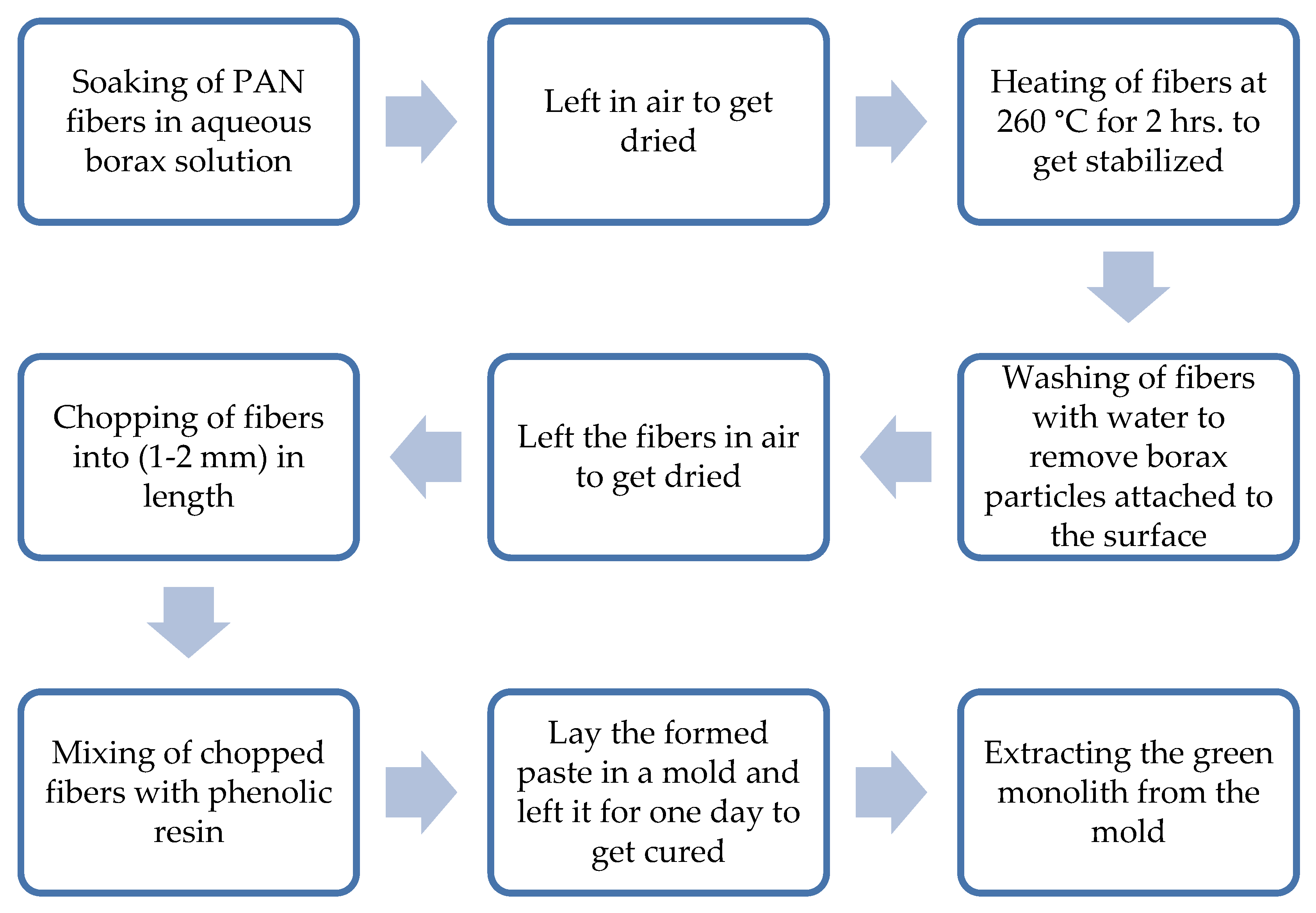
Figure 1.
Steps of preparation of the composite green monolith. Note: The green monolith was laid under a pressure of 14 N/cm2 for eighteen hours at room temperature during the curing process for all the chemically activated samples, while the physically activated samples were not pressed. This was intended to observe the combination effect of pressing and chemical activation of the composite electrode.
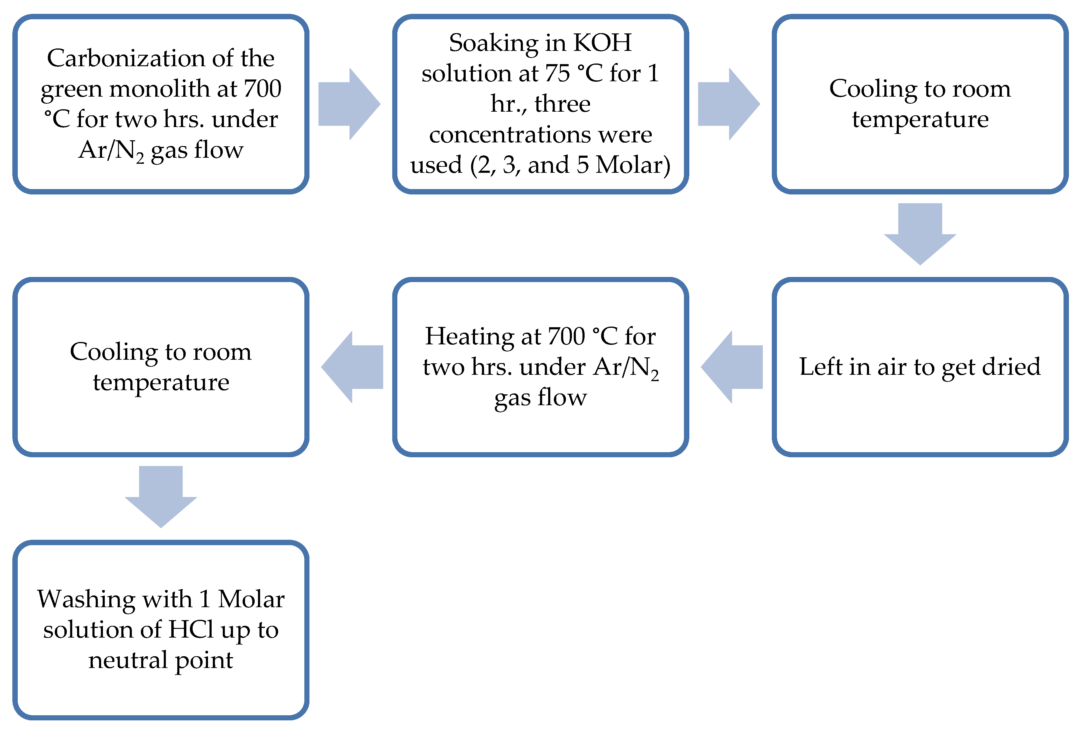
Figure 2.
Steps of chemical activation of the composite green monolith.
Figure 2.
Steps of chemical activation of the composite green monolith.
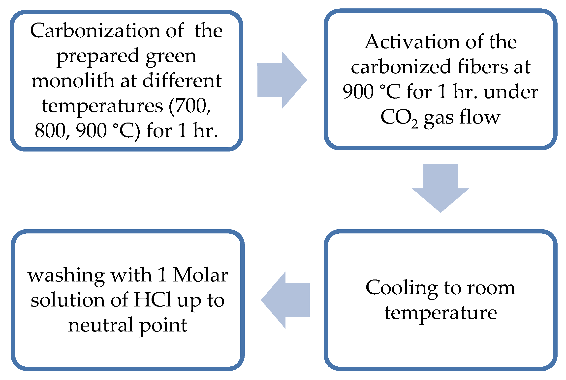
Figure 3.
Steps of physical activation of the composite green monolith.
Figure 3.
Steps of physical activation of the composite green monolith.
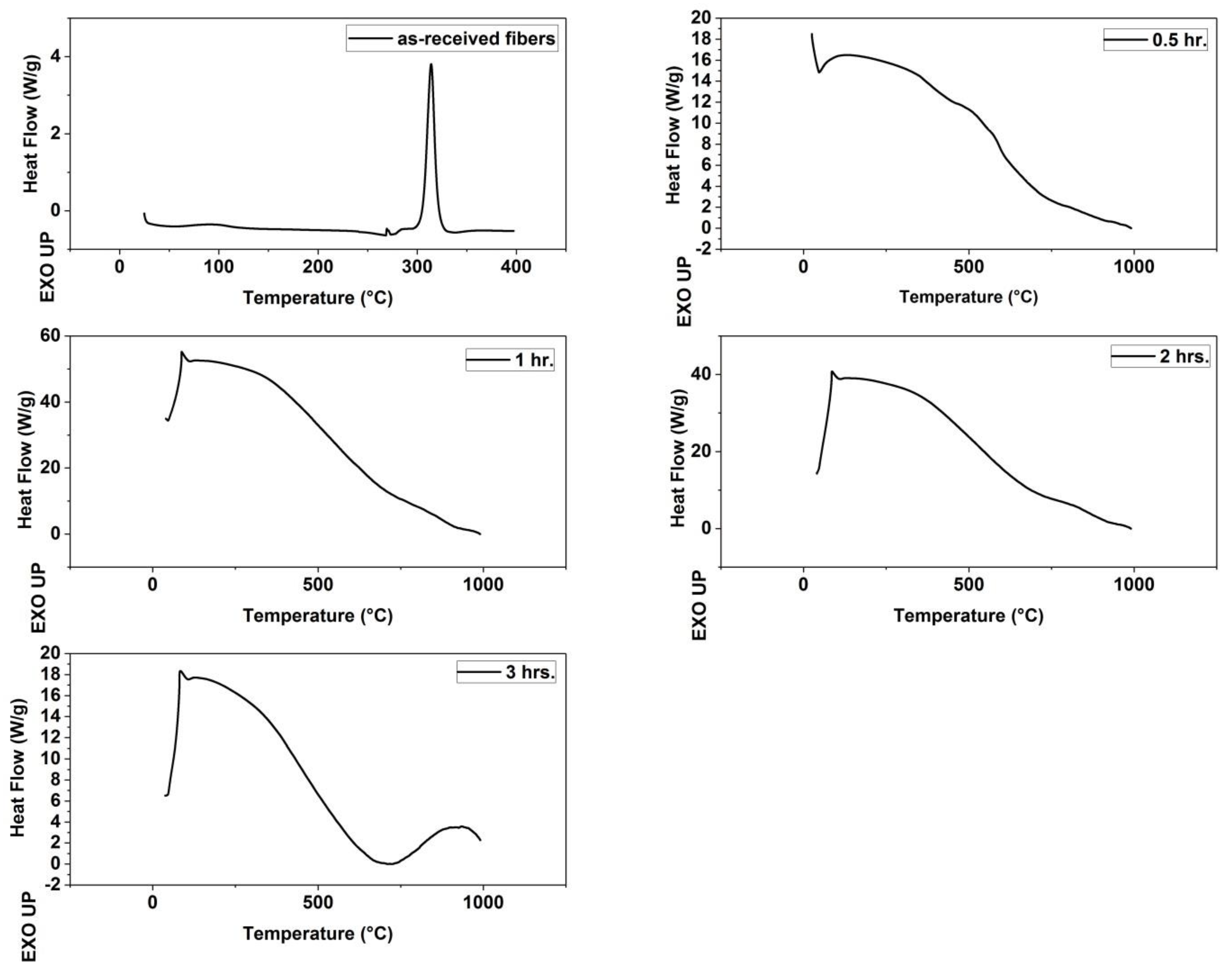
Figure 4.
Differential scanning calorimetry (DSC) Thermograms of (as-received fibers, fibers stabilized for 0.5 h, fibers stabilized for 1 h, fibers stabilized for 2 h and fibers stabilized for 3 h).
Figure 4.
Differential scanning calorimetry (DSC) Thermograms of (as-received fibers, fibers stabilized for 0.5 h, fibers stabilized for 1 h, fibers stabilized for 2 h and fibers stabilized for 3 h).
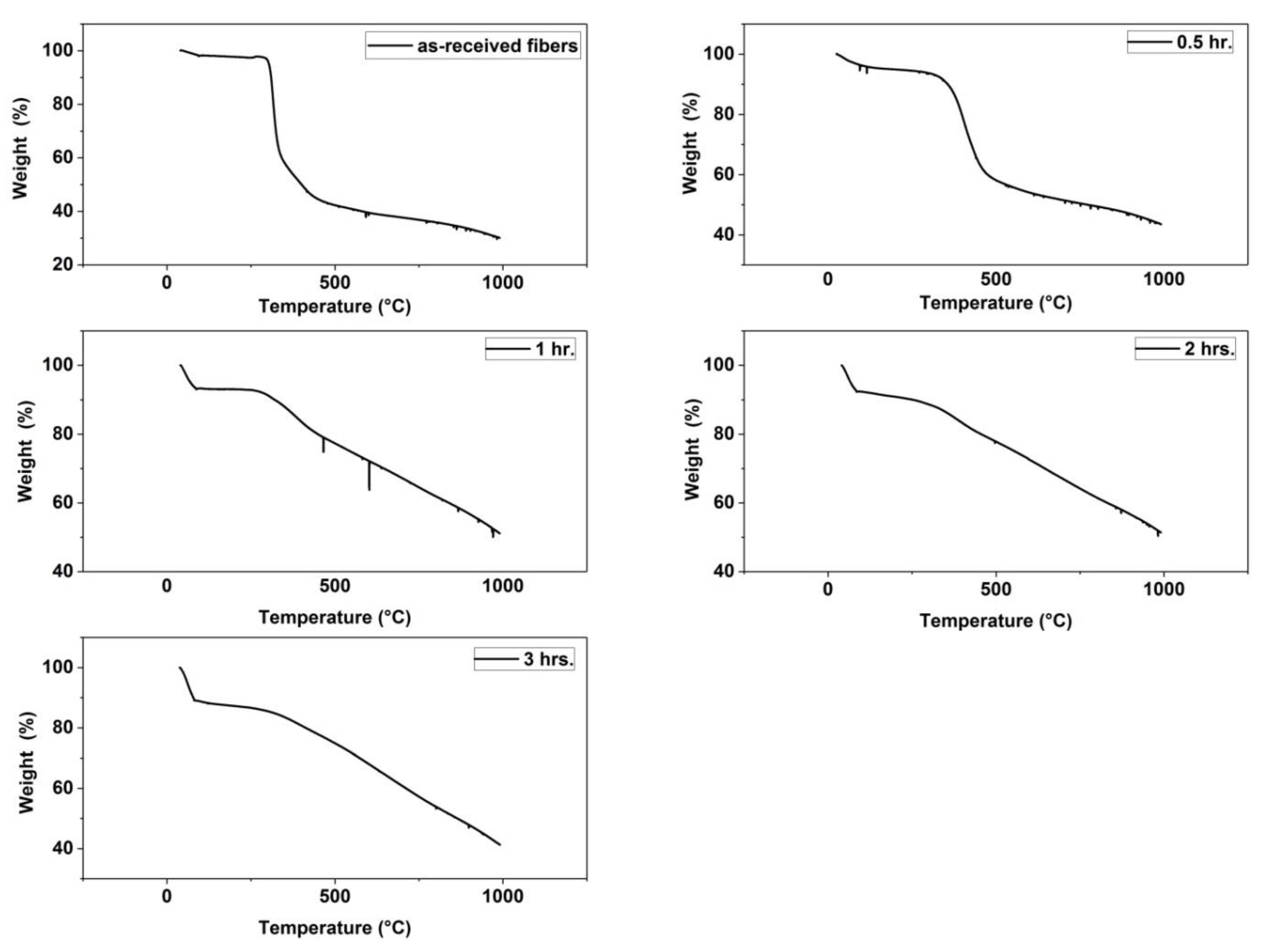
Figure 5.
Thermal gravimetric analysis (TGA) Thermograms of (as-received fibers, fibers stabilized for 0.5 h, fibers stabilized for 1 h, fibers stabilized for 2 h and fibers stabilized for 3 h).
Figure 5.
Thermal gravimetric analysis (TGA) Thermograms of (as-received fibers, fibers stabilized for 0.5 h, fibers stabilized for 1 h, fibers stabilized for 2 h and fibers stabilized for 3 h).
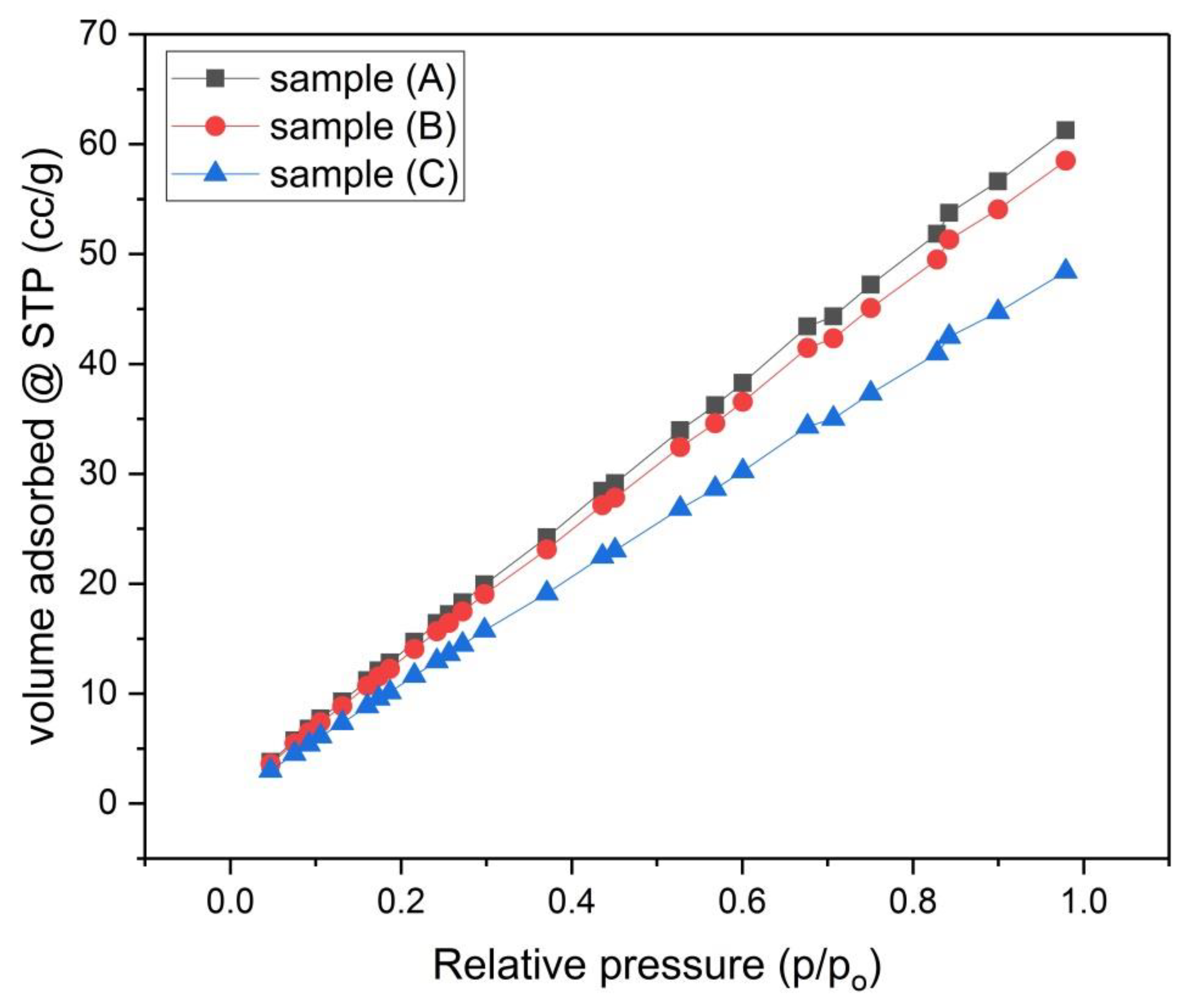
Figure 6.
N2 Adsorption Isotherms for samples (A), (B) and (C).
Figure 6.
N2 Adsorption Isotherms for samples (A), (B) and (C).
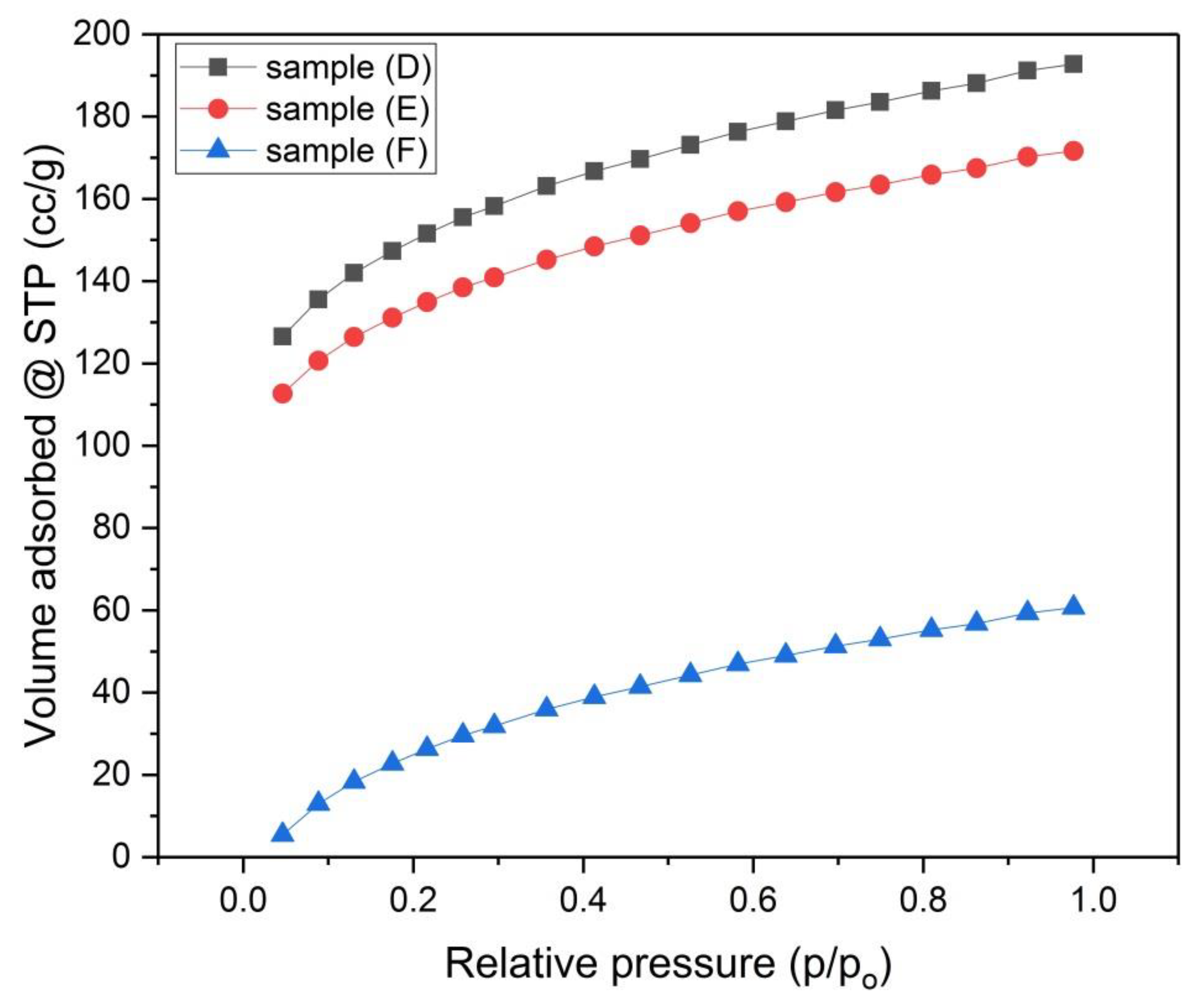
Figure 7.
N2-Adsorption Isotherms for samples (D), (E) and (F).
Figure 7.
N2-Adsorption Isotherms for samples (D), (E) and (F).
Figure 8.
Micropore size distribution by the Dubinin–Astakhov (DA) method for samples (A), (B) and (C).
Figure 8.
Micropore size distribution by the Dubinin–Astakhov (DA) method for samples (A), (B) and (C).
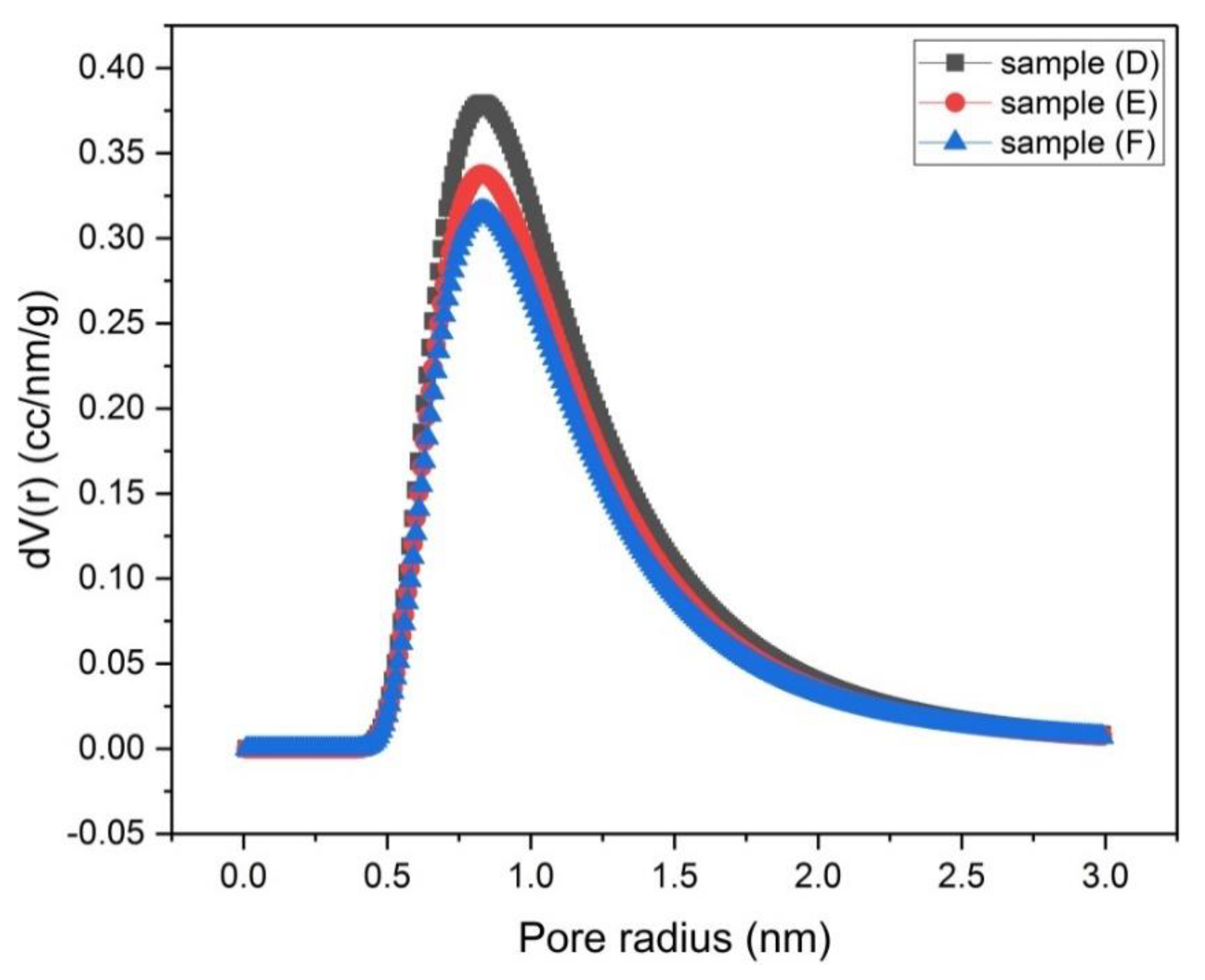
Figure 9.
Micropore size distribution by the DA method for samples (D), (E) and (F).
Figure 9.
Micropore size distribution by the DA method for samples (D), (E) and (F).
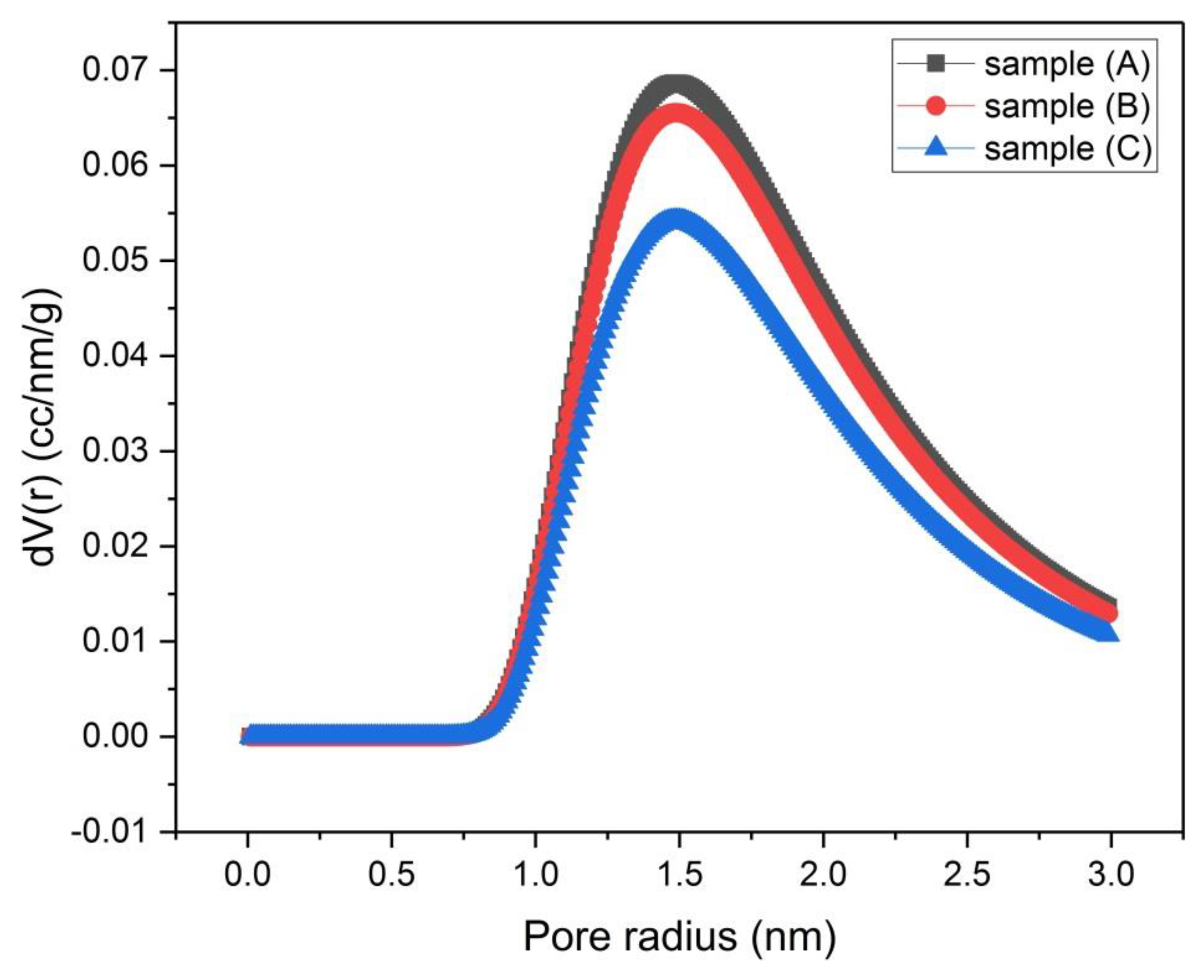
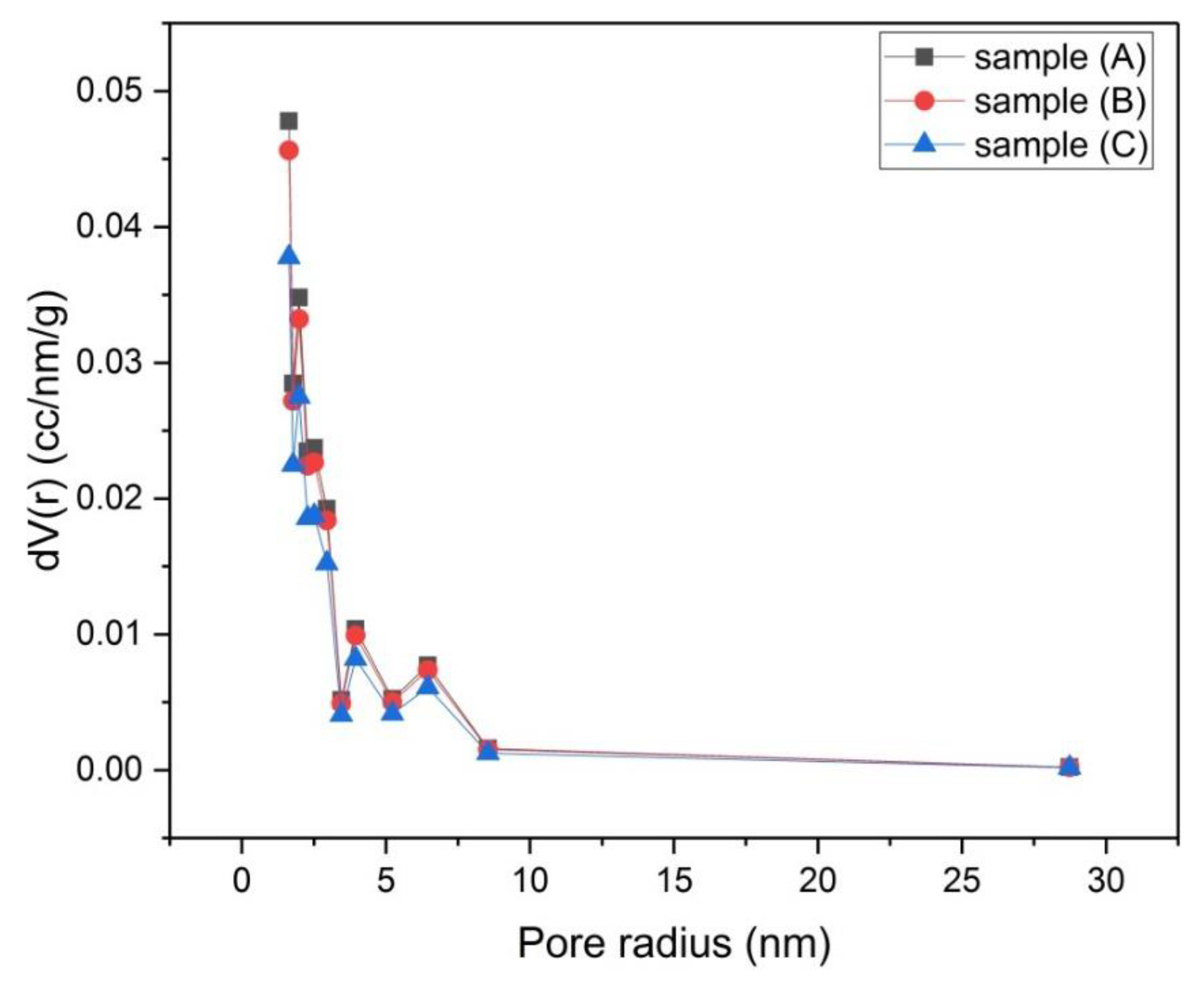
Figure 10.
Mesopore size distribution by the Barrett–Joyner–Halenda (BJH) method for samples (A), (B) and (C).
Figure 10.
Mesopore size distribution by the Barrett–Joyner–Halenda (BJH) method for samples (A), (B) and (C).
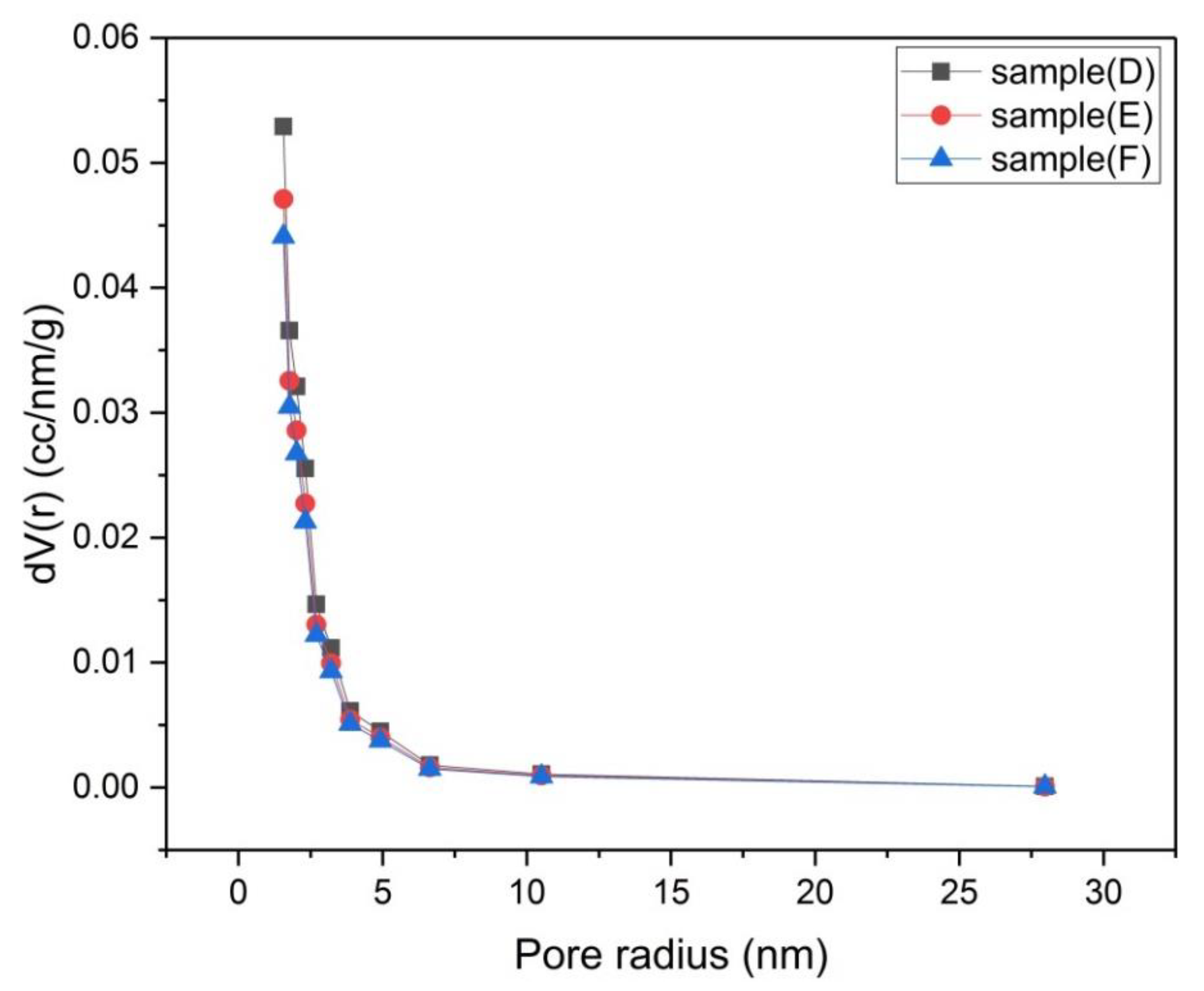
Figure 11.
Mesopore size distribution by BJH method for samples (D), (E) and (F).
Figure 11.
Mesopore size distribution by BJH method for samples (D), (E) and (F).
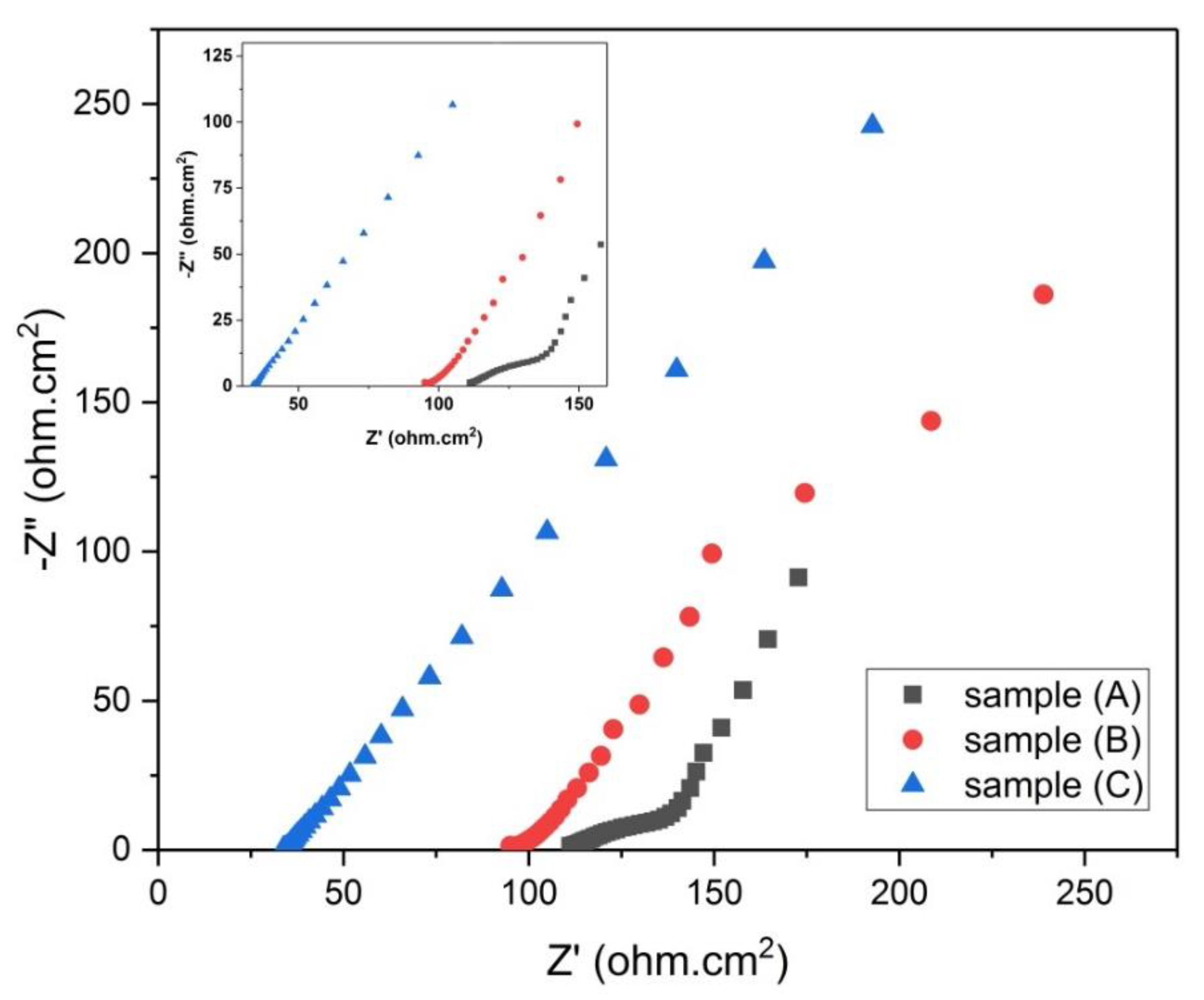
Figure 12.
Nyquist plot for samples (A, B and C).
Figure 12.
Nyquist plot for samples (A, B and C).
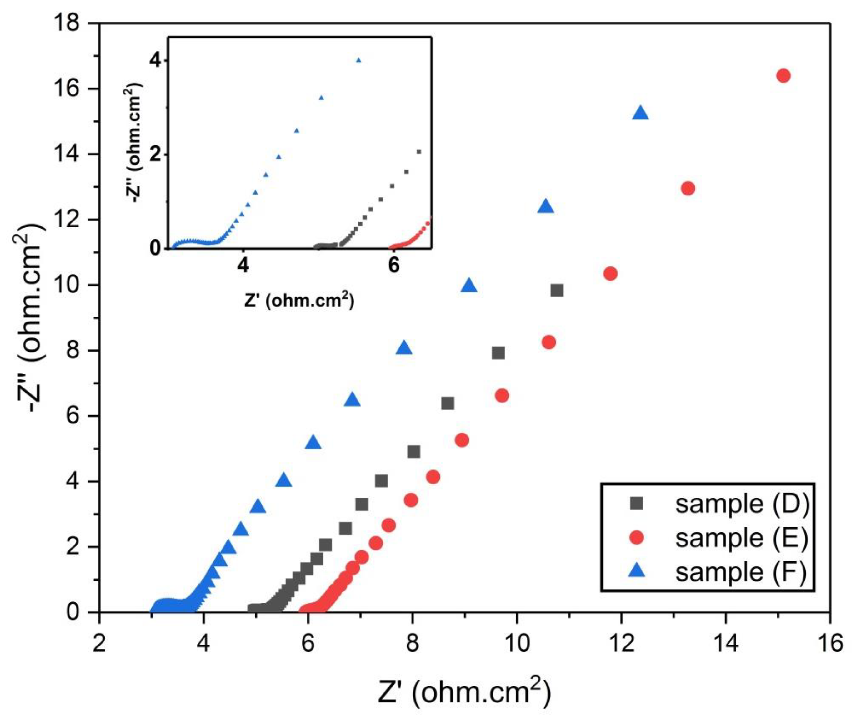
Figure 13.
Nyquist plot for samples (D, E, and F).
Figure 13.
Nyquist plot for samples (D, E, and F).
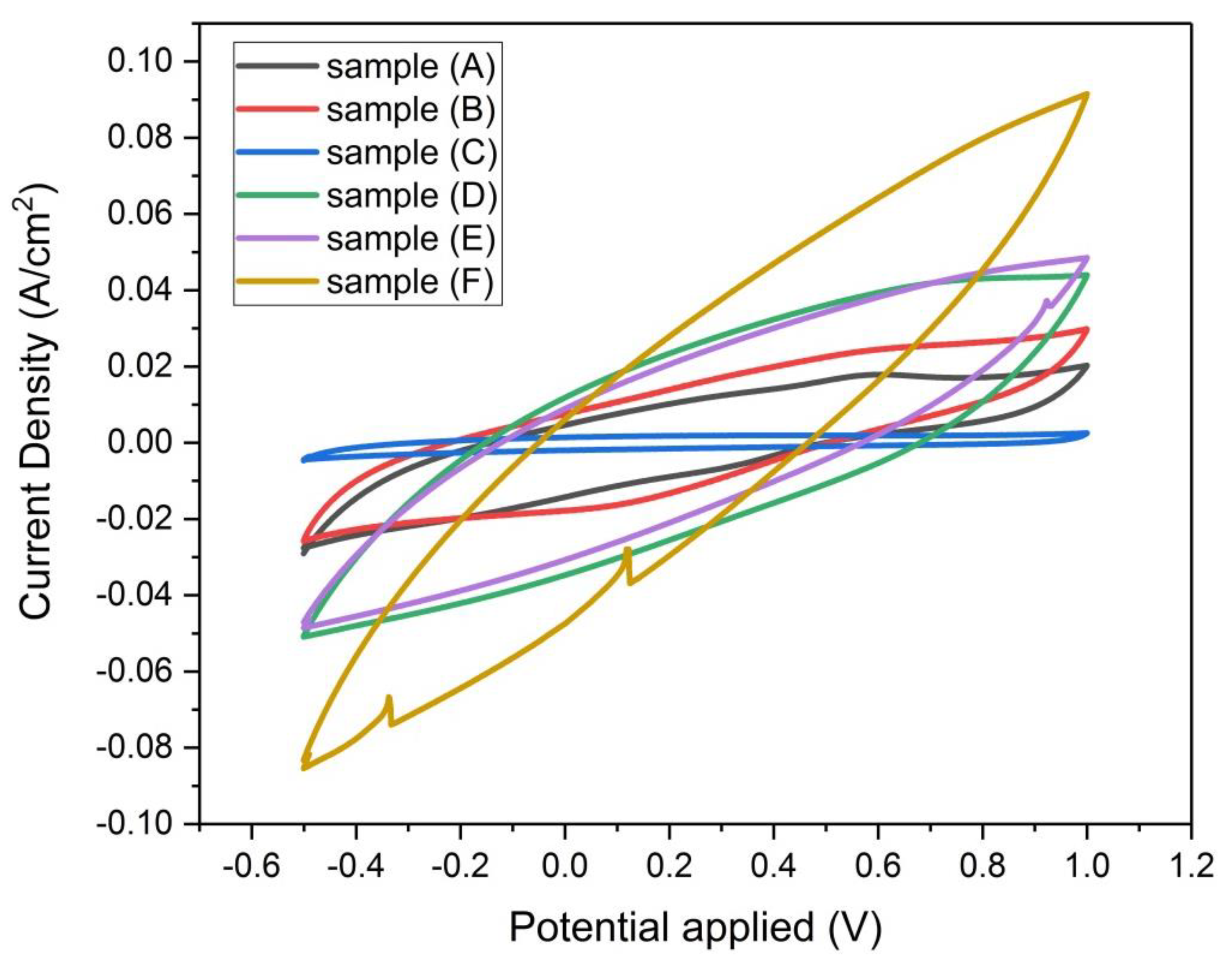
Figure 14.
Cyclic Voltammograms of samples (A, B, C, D, E, and F) at scan rate 100 mv/sec, based on three-electrode measurement with 2 Molar H2SO4 solution.
Figure 14.
Cyclic Voltammograms of samples (A, B, C, D, E, and F) at scan rate 100 mv/sec, based on three-electrode measurement with 2 Molar H2SO4 solution.
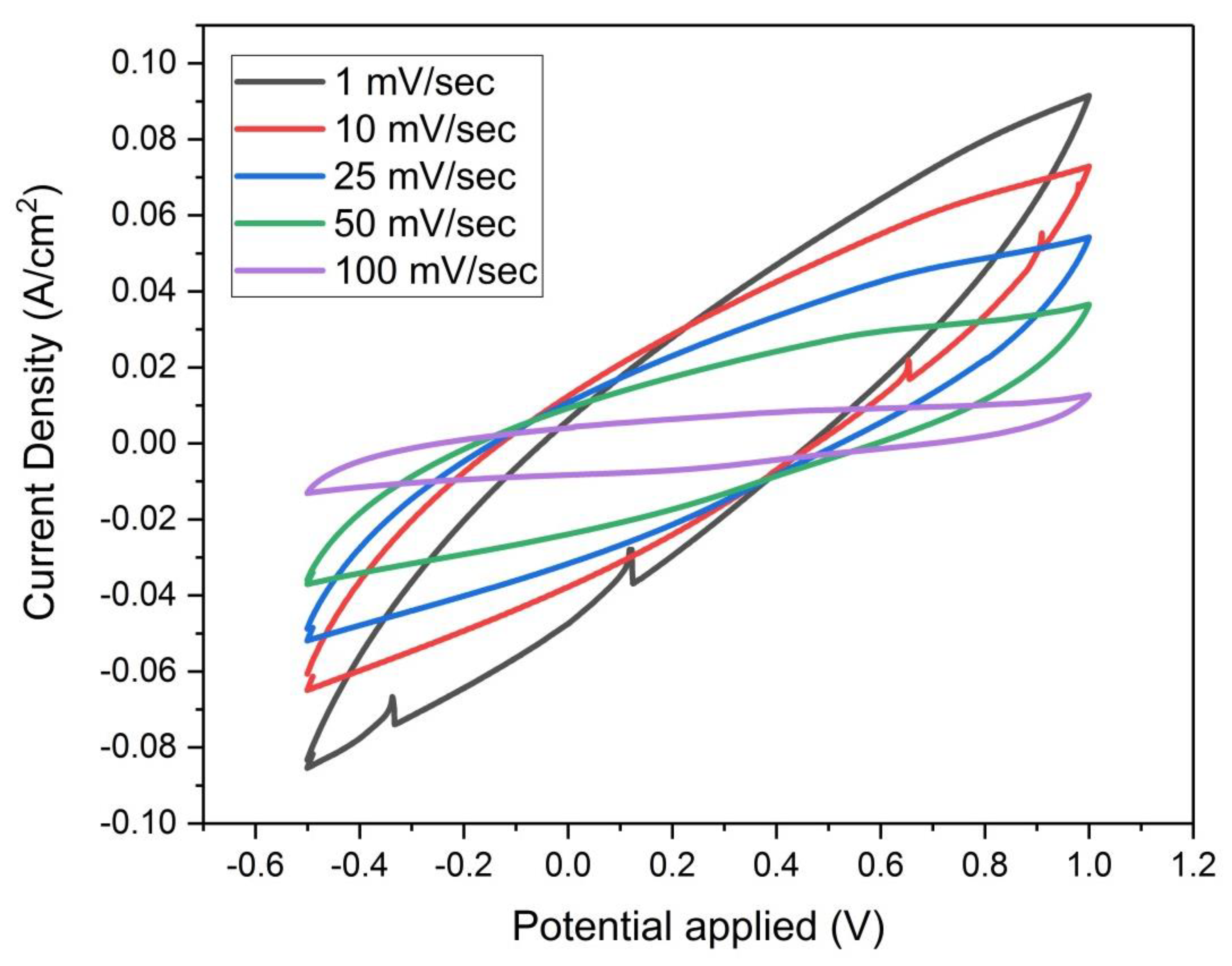
Figure 15.
Cyclic Voltammograms of sample (F) at scan rates (1, 10, 25, 50 and 100 mV/sec), based on three-electrode measurement with 2 Molar H2SO4 solution.
Figure 15.
Cyclic Voltammograms of sample (F) at scan rates (1, 10, 25, 50 and 100 mV/sec), based on three-electrode measurement with 2 Molar H2SO4 solution.
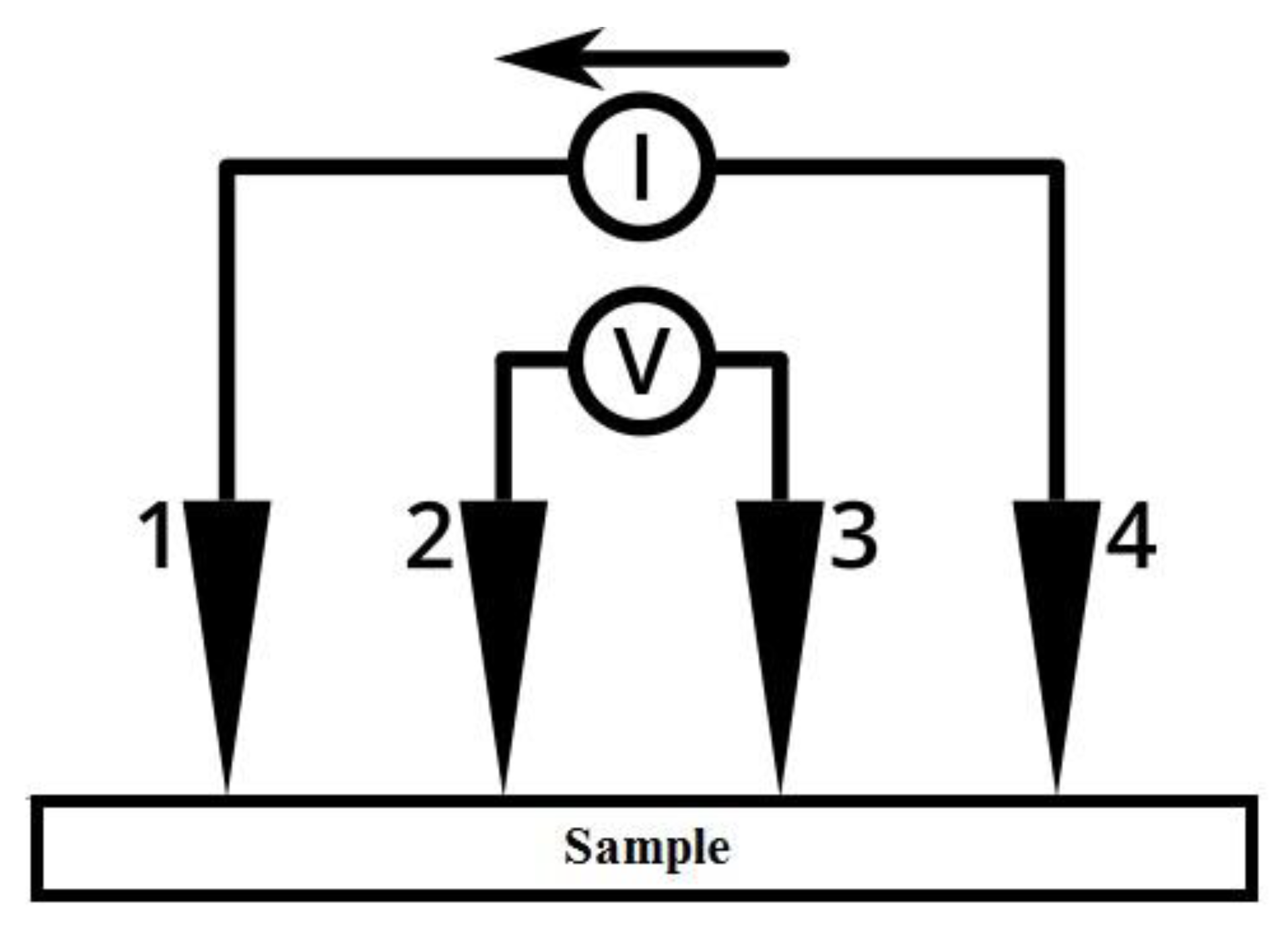
Figure 16.
Four-point probe measurement principle.
Figure 16.
Four-point probe measurement principle.
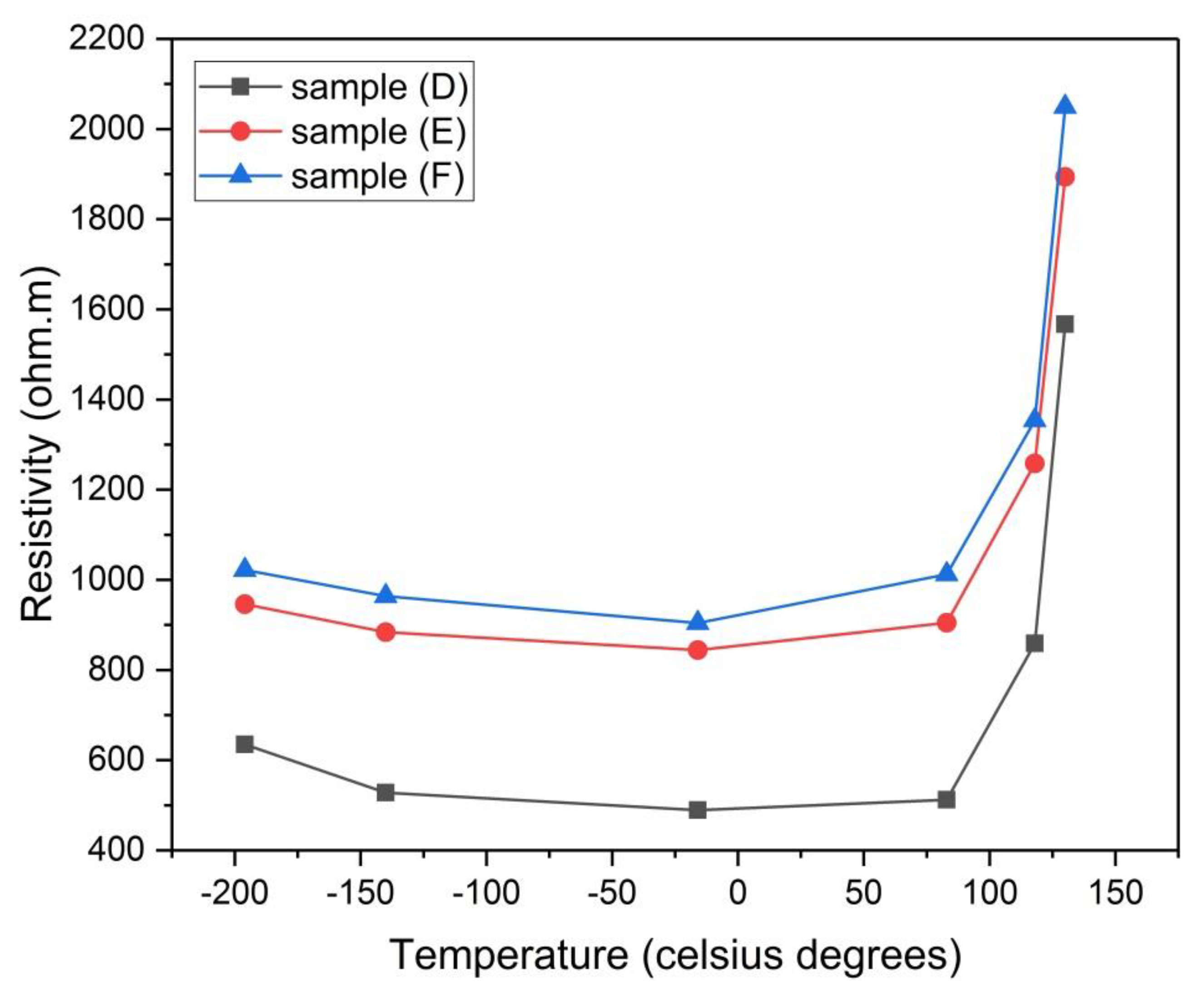
Figure 17.
Electrical resistivity of samples (D), (E) and (F) versus the temperature of analysis.
Figure 17.
Electrical resistivity of samples (D), (E) and (F) versus the temperature of analysis.
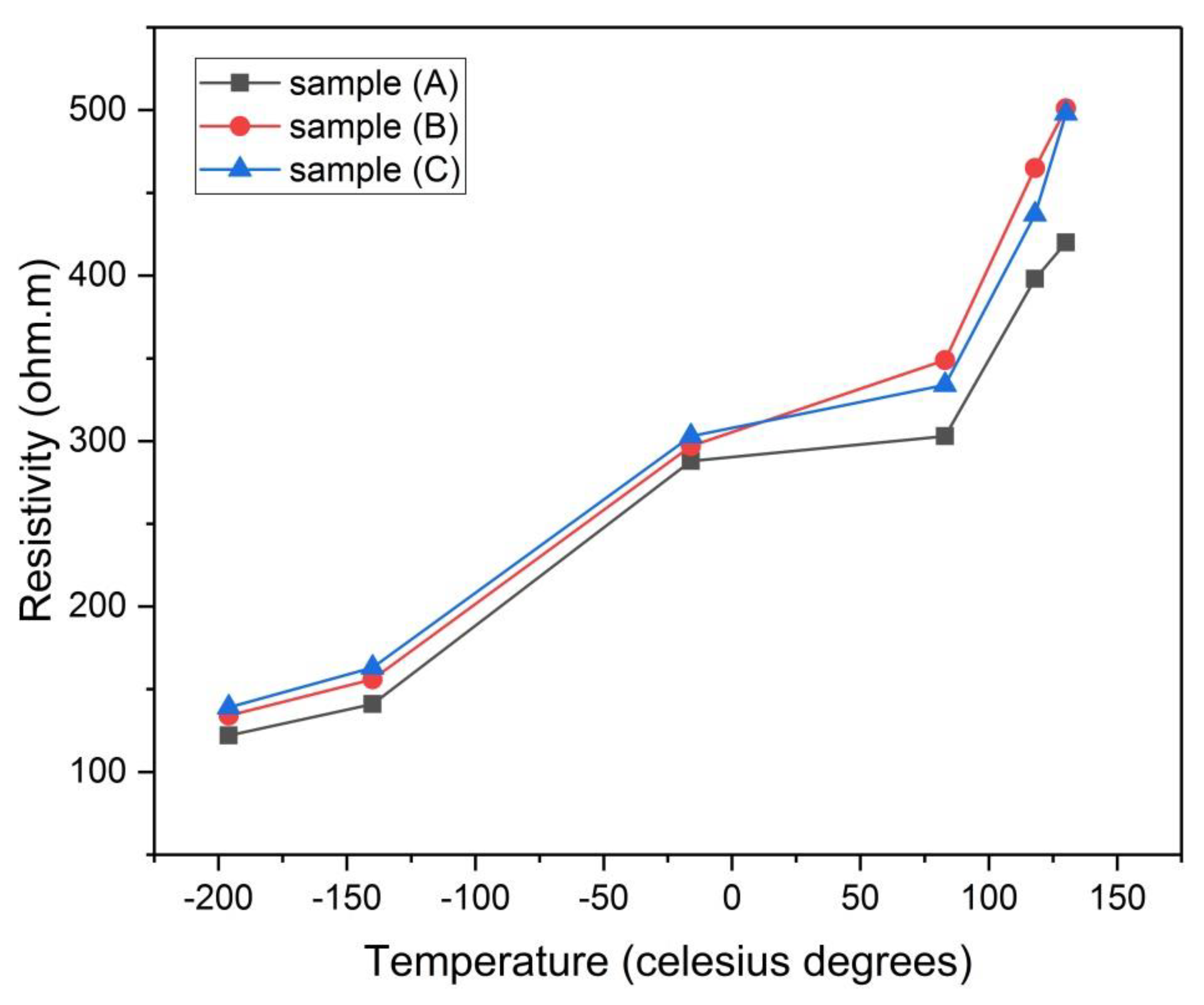
Figure 18.
Electrical resistivity of samples (A), (B), and (C) versus the temperature of analysis.
Figure 18.
Electrical resistivity of samples (A), (B), and (C) versus the temperature of analysis.
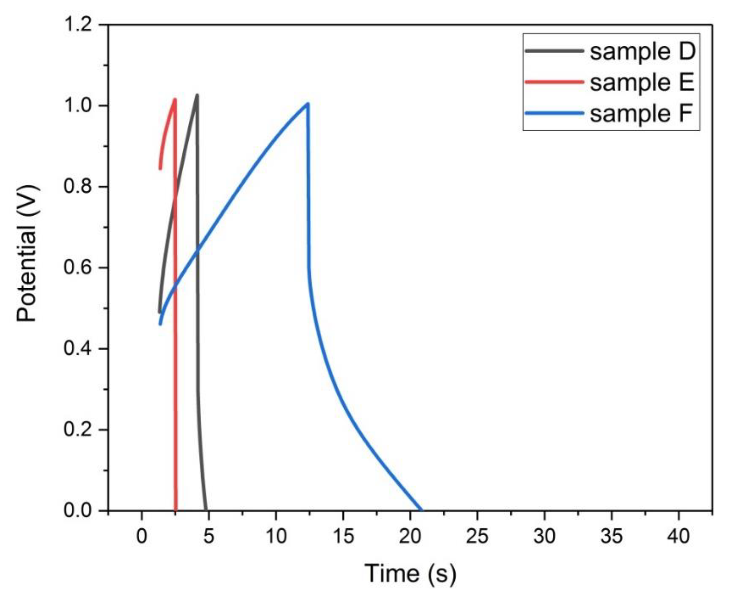
Figure 19.
Galvanostatic charge–discharge plots of samples (D, E, and F) at 50 mA/g.
Figure 19.
Galvanostatic charge–discharge plots of samples (D, E, and F) at 50 mA/g.
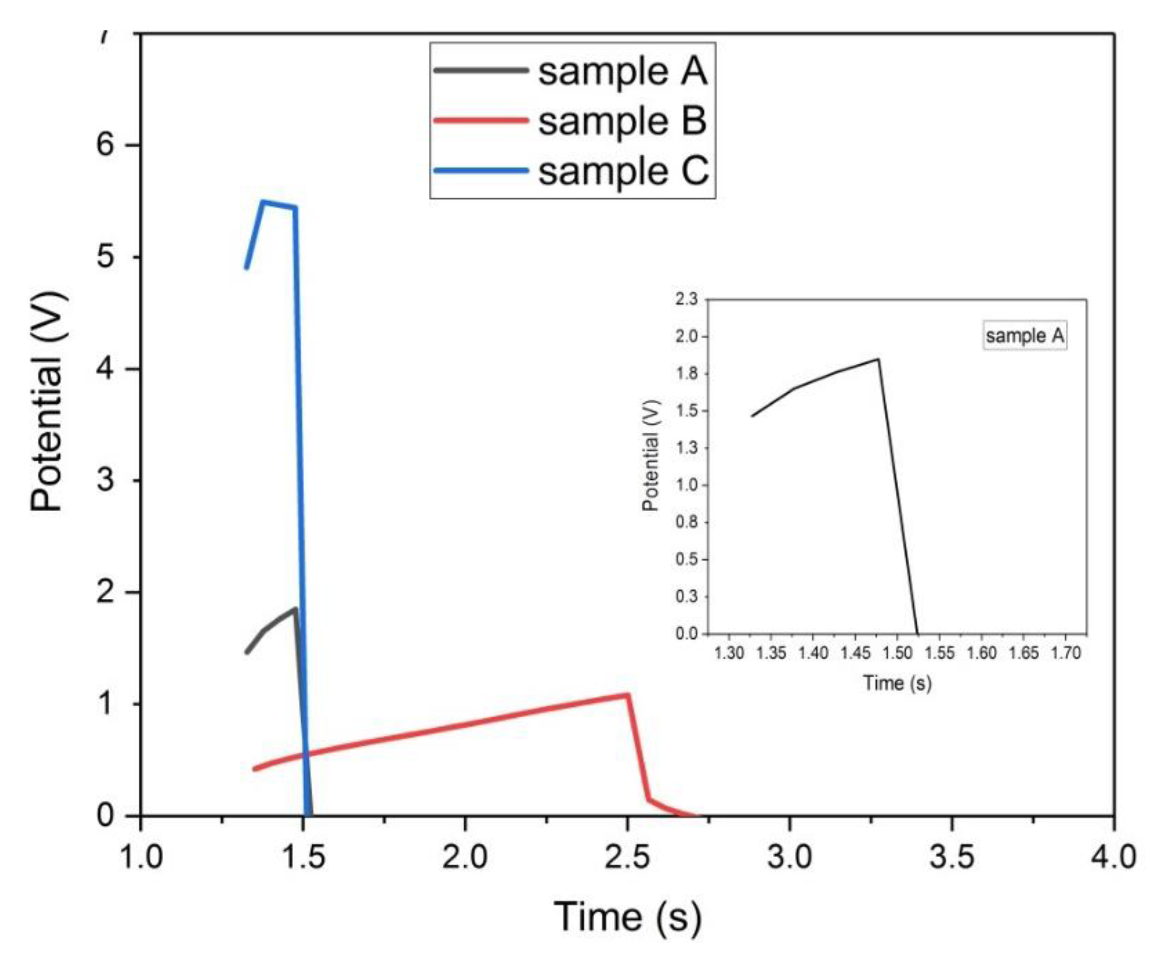
Figure 20.
Galvanostatic charge-discharge plots of samples (A, B, and C) at 50 mA/g.
Figure 20.
Galvanostatic charge-discharge plots of samples (A, B, and C) at 50 mA/g.
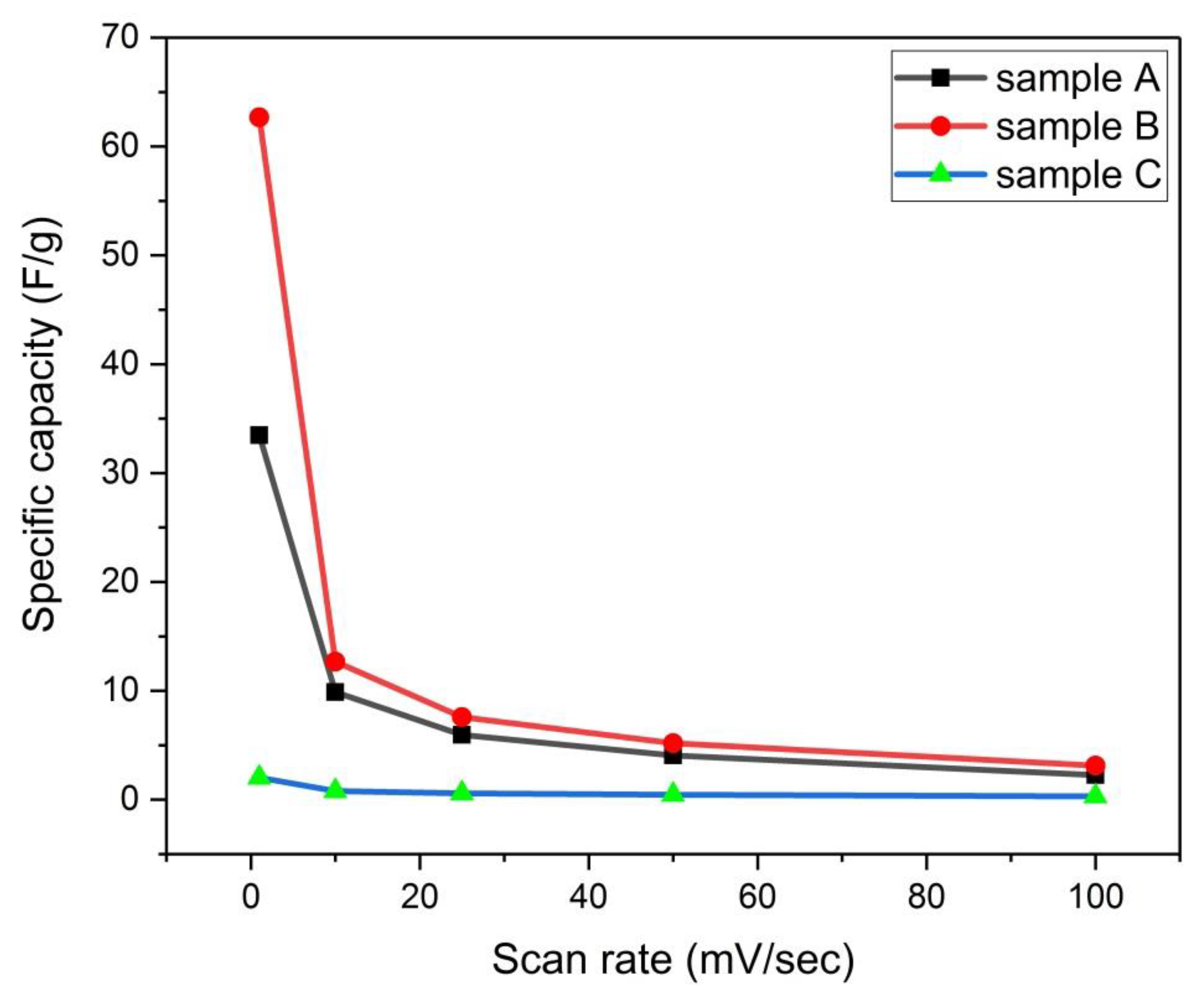
Figure 21.
Variation of specific capacity with scan rate for samples (A, B, and C).
Figure 21.
Variation of specific capacity with scan rate for samples (A, B, and C).
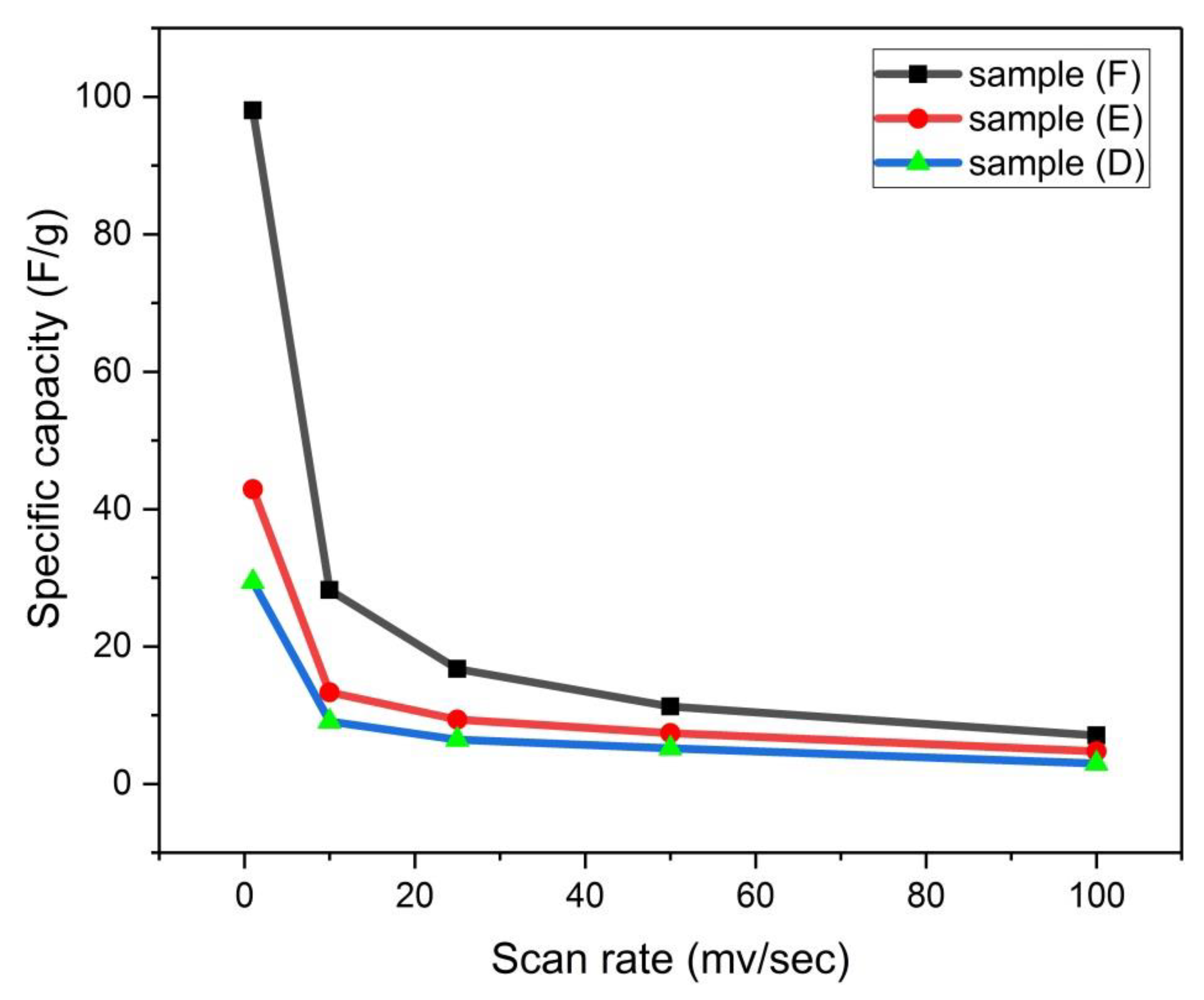
Figure 22.
Variation of specific capacity with scan rate for samples (D, E, and F).
Figure 22.
Variation of specific capacity with scan rate for samples (D, E, and F).
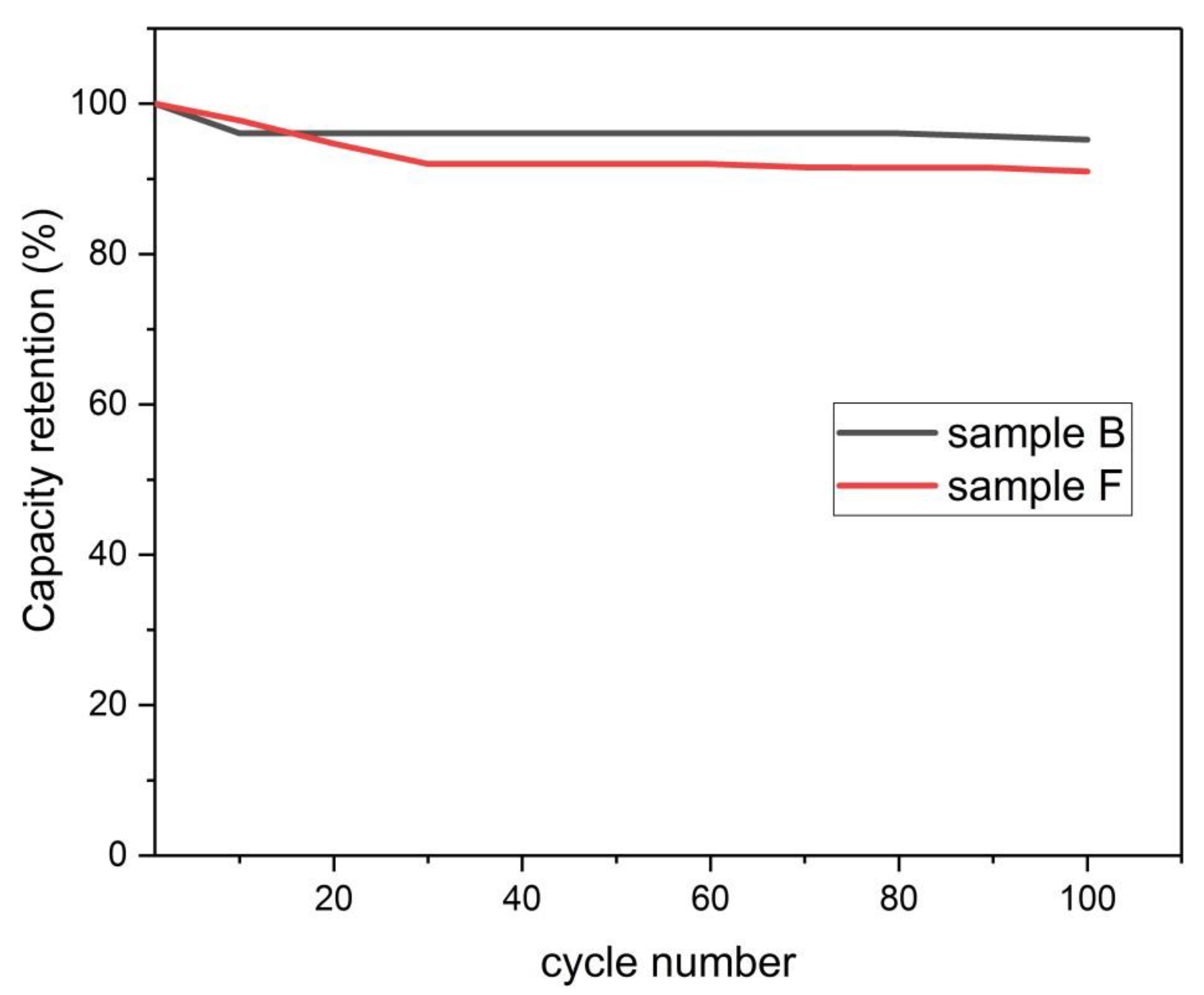
Figure 23.
Capacity retention versus cycle number.
Figure 23.
Capacity retention versus cycle number.
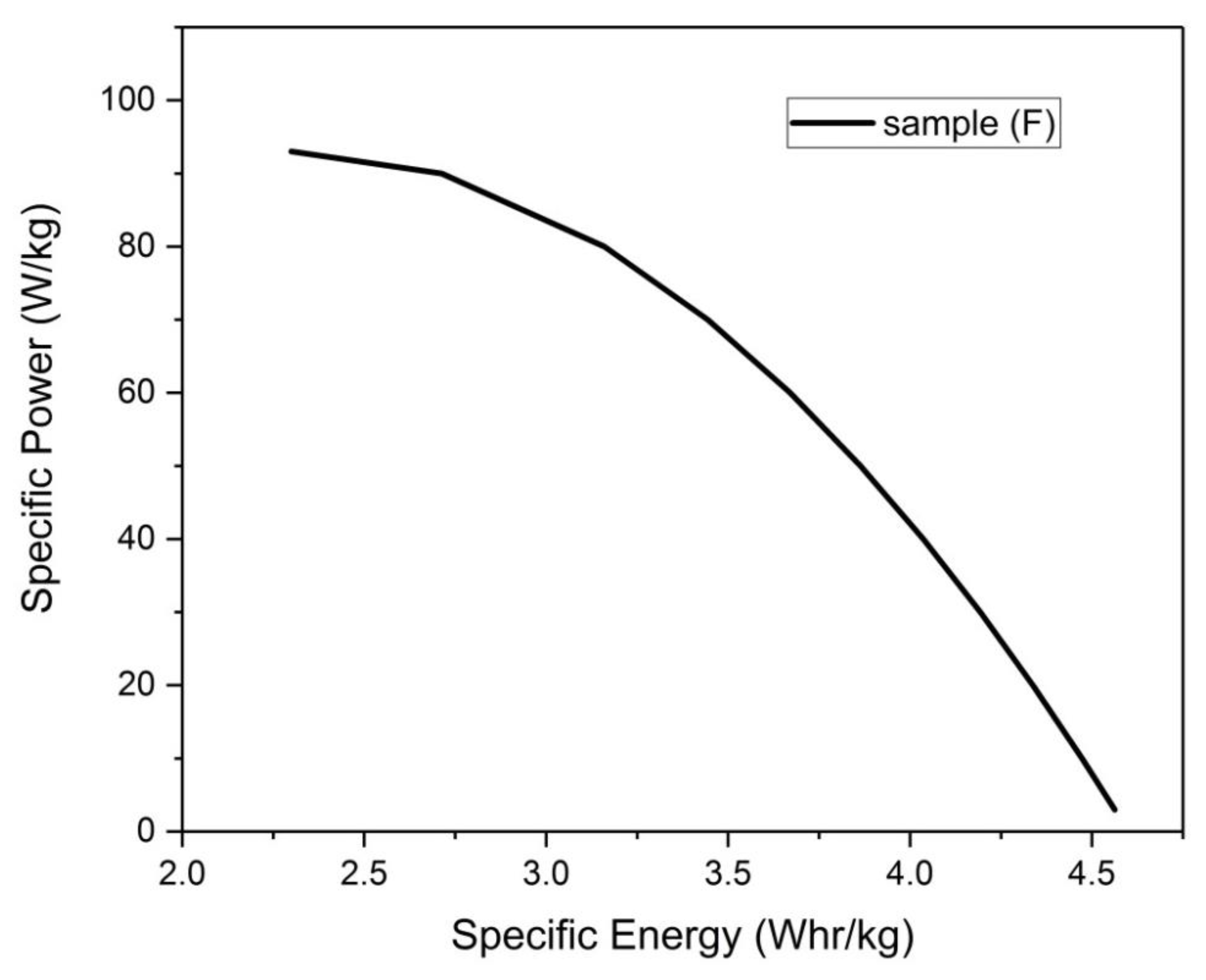
Figure 24.
Ragone plot for sample (F).
Figure 24.
Ragone plot for sample (F).
Table 1.
DSC data of as-received fibers.
Table 1.
DSC data of as-received fibers.
| Type of Fibers | Energy Released (J/g) | Temperature at the Start of the Exothermic Peak (°C) | Temperature at the Vertex of the Exothermic Peak (°C) |
|---|
| As-received Fibers | 251.3 | 305.91 | 314.06 |
Table 2.
Residual weights of the as-received fibers and thermally stabilized fibers.
Table 2.
Residual weights of the as-received fibers and thermally stabilized fibers.
| Sample | Residual Weight (%) |
|---|
| As-received fibers | 30.125 |
| Fibers resided for 0.5 h in furnace | 43.56 |
| Fibers resided for 1 h in furnace | 51.1 |
| Fibers resided for 2 h in furnace | 51.4 |
| Fibers resided for 3 h in furnace | 41.6 |
Table 3.
Elemental Analysis of as-received fibers and thermally stabilized fibers.
Table 3.
Elemental Analysis of as-received fibers and thermally stabilized fibers.
| Sample | C % | H % | N % | C/H | C/N |
|---|
| As-received fibers | 66.55 | 5.43 | 16.27 | 12.25 | 4.1 |
| Fibers treated for 0.5h | 71.28 | 6.14 | 18.99 | 11.6 | 3.75 |
| Fibers treated for 1 h | 70.27 | 3.2 | 26.46 | 21.95 | 2.65 |
| Fibers treated for 2 h | 57.34 | 1.4 | 20.25 | 40.96 | 2.83 |
| Fibers treated for 3 h | 65.12 | 4.3 | 23.09 | 15.14 | 2.82 |
Table 4.
Porous Structure Characteristics.
Table 4.
Porous Structure Characteristics.
| Sample | SBET (m2/g) | Smicro (m2/g) | Smeso (m2/g) | Vmicro (cc/g) | Vmeso (cc/g) | Vtotal (cc/g) | Vmicro/Vmeso |
|---|
| (A) | 100 | 42.76 | 57.24 | 0.0053 | 0.085 | 0.0903 | 0.062 |
| (B) | 95 | 41 | 54 | 0.0095 | 0.0812 | 0.0907 | 0.12 |
| (C) | 79 | 34 | 45 | 0.008 | 0.067 | 0.075 | 0.12 |
| (D) | 486 | 435 | 51 | 0.226 | 0.073 | 0.299 | 3.1 |
| (E) | 433 | 387 | 46 | 0.202 | 0.064 | 0.266 | 3.2 |
| (F) | 405 | 362 | 43 | 0.189 | 0.060 | 0.249 | 3.2 |
Table 5.
The ESR and Rct values for different samples.
Table 5.
The ESR and Rct values for different samples.
| Sample | ESR (ohm/cm2) | Rct (ohm/cm2) |
|---|
| A | 33.88 | - |
| B | 29 | - |
| C | 11.74 | - |
| D | 1.36 | 0.049 |
| E | 1.18 | 0.028 |
| F | 1.73 | 0.248 |
Table 6.
Csp for Different Samples and their Corresponding SBET.
Table 6.
Csp for Different Samples and their Corresponding SBET.
| Sample | Csp (F/g) | SBET (m2/g) |
|---|
| A | 6.0 | 100 |
| B | 5.12 | 95 |
| C | 0.78 | 79 |
| D | 7.28 | 486 |
| E | 9.94 | 433 |
| F | 29.25 | 405 |
Table 7.
Electrical Resistivity of Different Samples at 25 °C.
Table 7.
Electrical Resistivity of Different Samples at 25 °C.
| Sample | Resistivity (Ω.m) |
|---|
| A | 294 |
| B | 293 |
| C | 303 |
| D | 500 |
| E | 932 |
| F | 1035 |
Table 8.
Emax and Pmax values of some composite monolith electrodes.
Table 8.
Emax and Pmax values of some composite monolith electrodes.
| Electrode | Emax (Whr/kg) | Pmax (W/kg) | Ref. |
|---|
| Textile grade PAN fibers/phenolic resin | 4.6 | 93 | Present study |
| activated carbon/graphene oxide | 6 | 30 | [20] |
| activated carbon/CNT | 11.25 | 3650 | [28] |
| activated carbon/graphene. | 8.5 | 25 | [29] |
Table 9.
SBET, Csp and ESR of various carbon electrodes.
Table 9.
SBET, Csp and ESR of various carbon electrodes.
| Type of Carbon Electrode | SBet (m2/g) | Csp (F/g) | ESR (Ω) | Reference |
|---|
| Activated carbon monolith | 405 | 29.25 | 2.3 | present study |
| Carbon nanotubes (CNT) | 430–1600 | 180 | 101 | [30,31] |
| Graphene sheets | 2630 | 150 | 96 | [30,32] |
| Activated carbon | 300–2749 | 100–233 | 0.5 | [32,33] |
| Carbide derived carbon | 1822 | 134 | 0.39 | [34] |
| Templated carbon | 1120 | 132 | 0.36–0.8 | [35] |
| Carbon Xerogel | 1243 | 234 | 33 | [36] |


