
Analysis of Cutting Stability of a Composite Variable-Section Boring Bar with a Large Length-to-Diameter Ratio Considering Internal Damping


Abstract
:1. Introduction
2. Free Vibration Control Equation and Solution to Vibration Characteristics
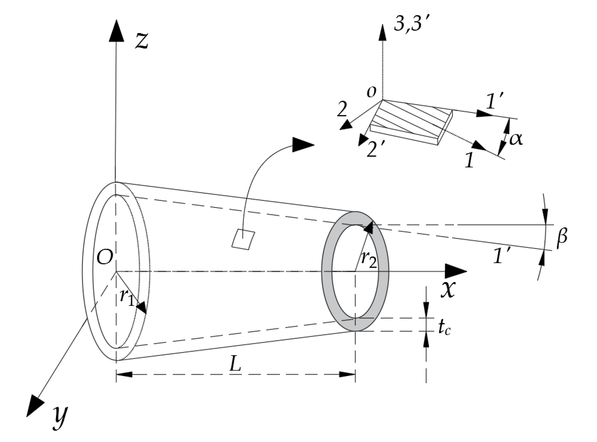
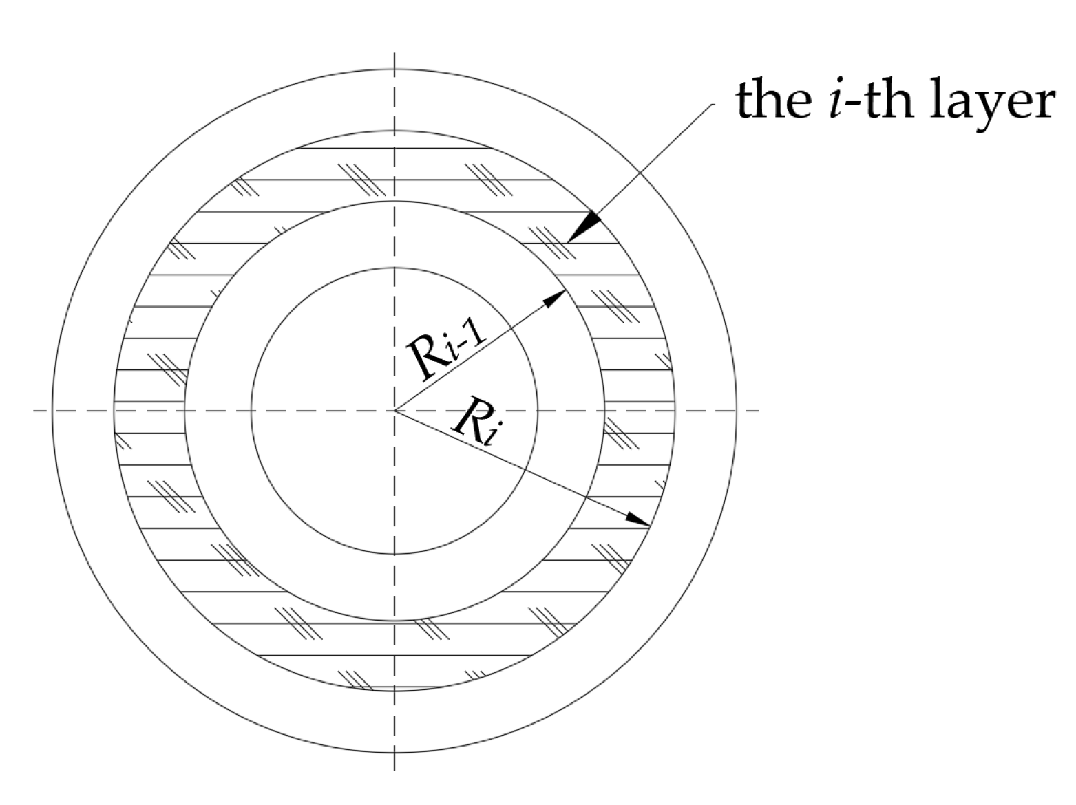
2.1. Constitutive Equation of the Boring Bar after the Consideration of Material Damping
2.2. Elastic Strain Energy of the Boring Bar
2.3. Kinetic Energy of the Boring Bar
2.4. Dissipated Virtual Work of the Boring Bar
2.5. Vibration Control Equation of the Boring Bar
2.6. Discrete Solution to Vibration Equation
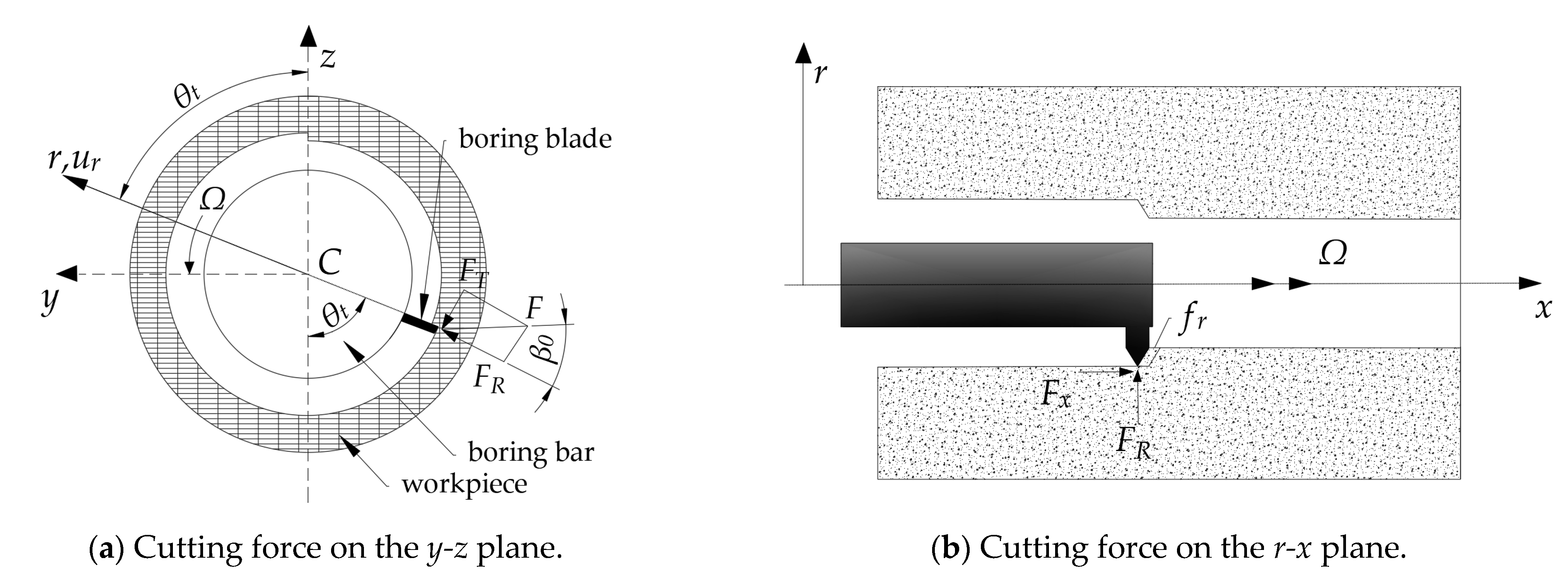
3. Boring Stability Analysis
4. Analysis of Numerical Results
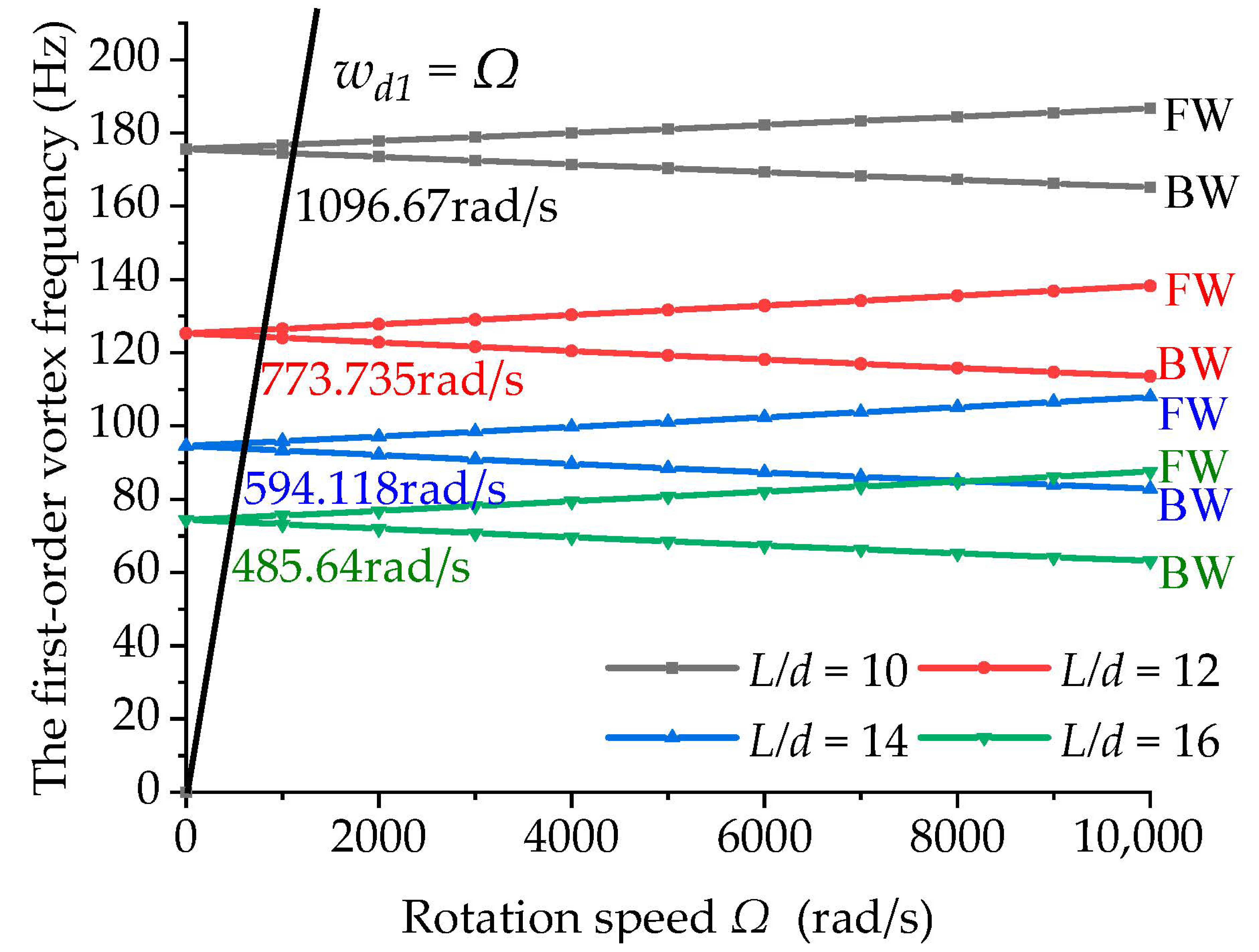
4.1. Natural Vibration Analysis
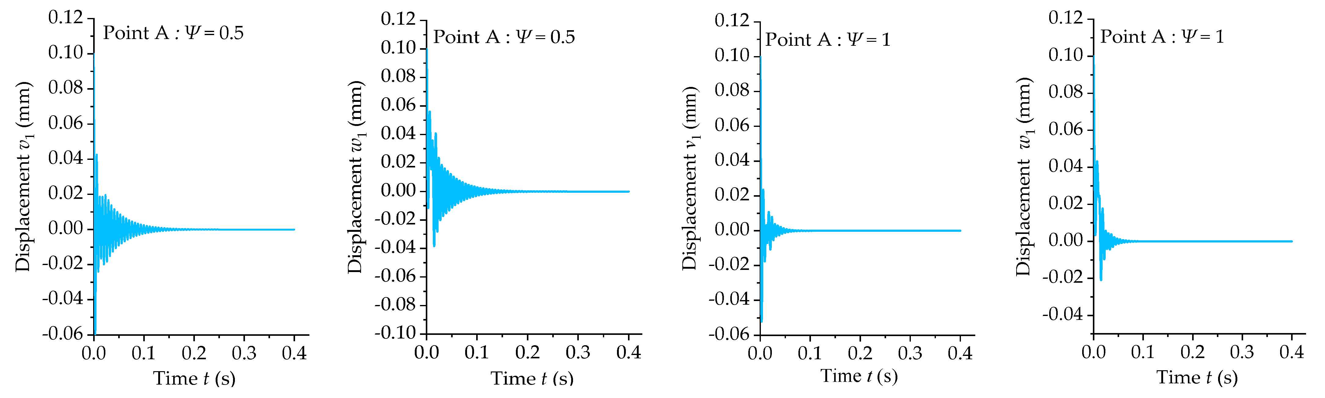
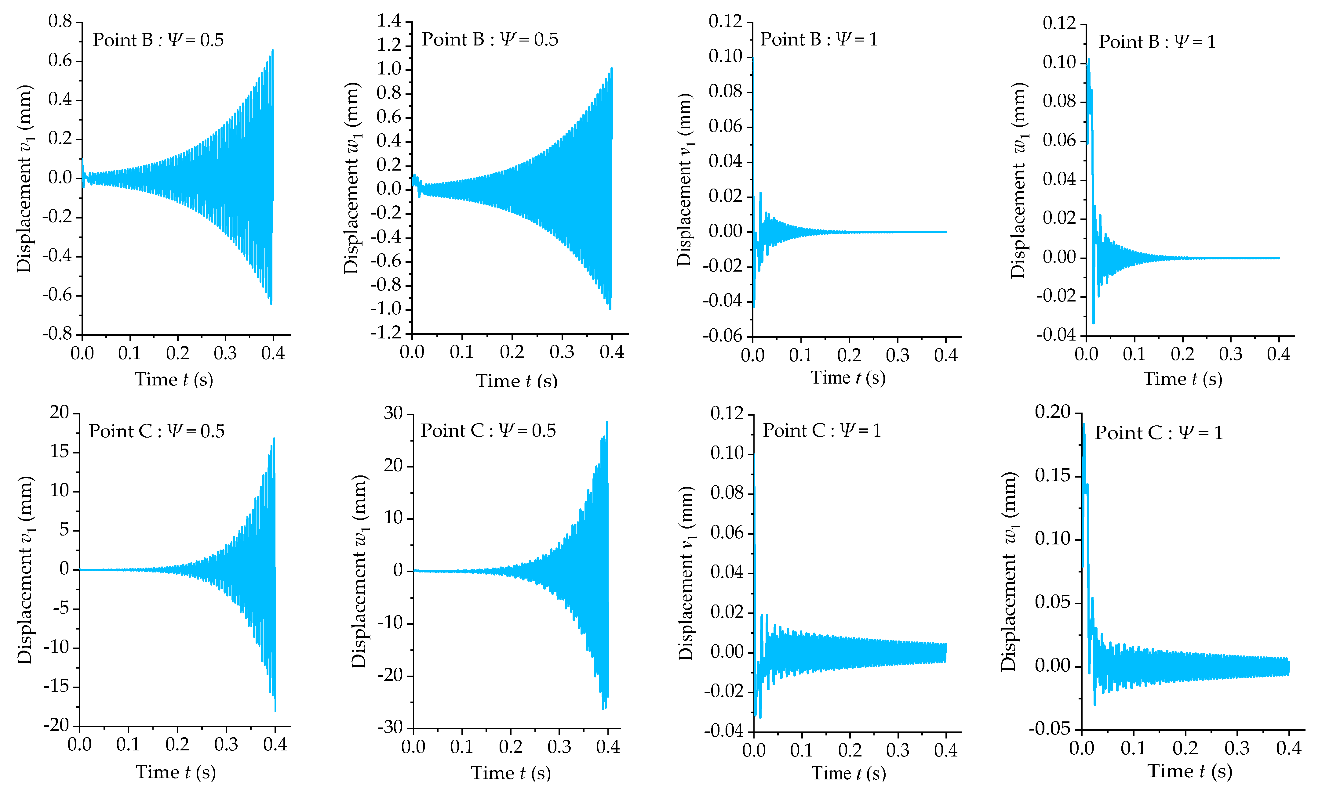
4.2. Cutting Stability Analysis
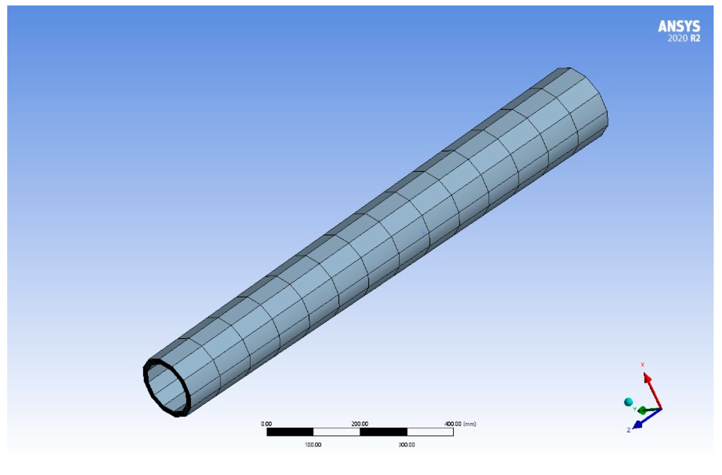
Validation of Model Reliability
4.3. Analysis of the Influencing Factors of the Boring Stability of the Boring Bar
5. Conclusions
- (1)
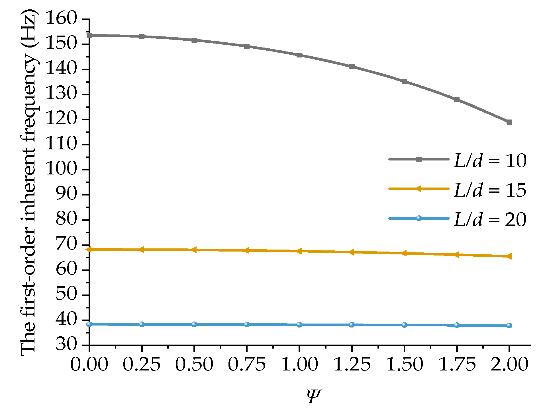
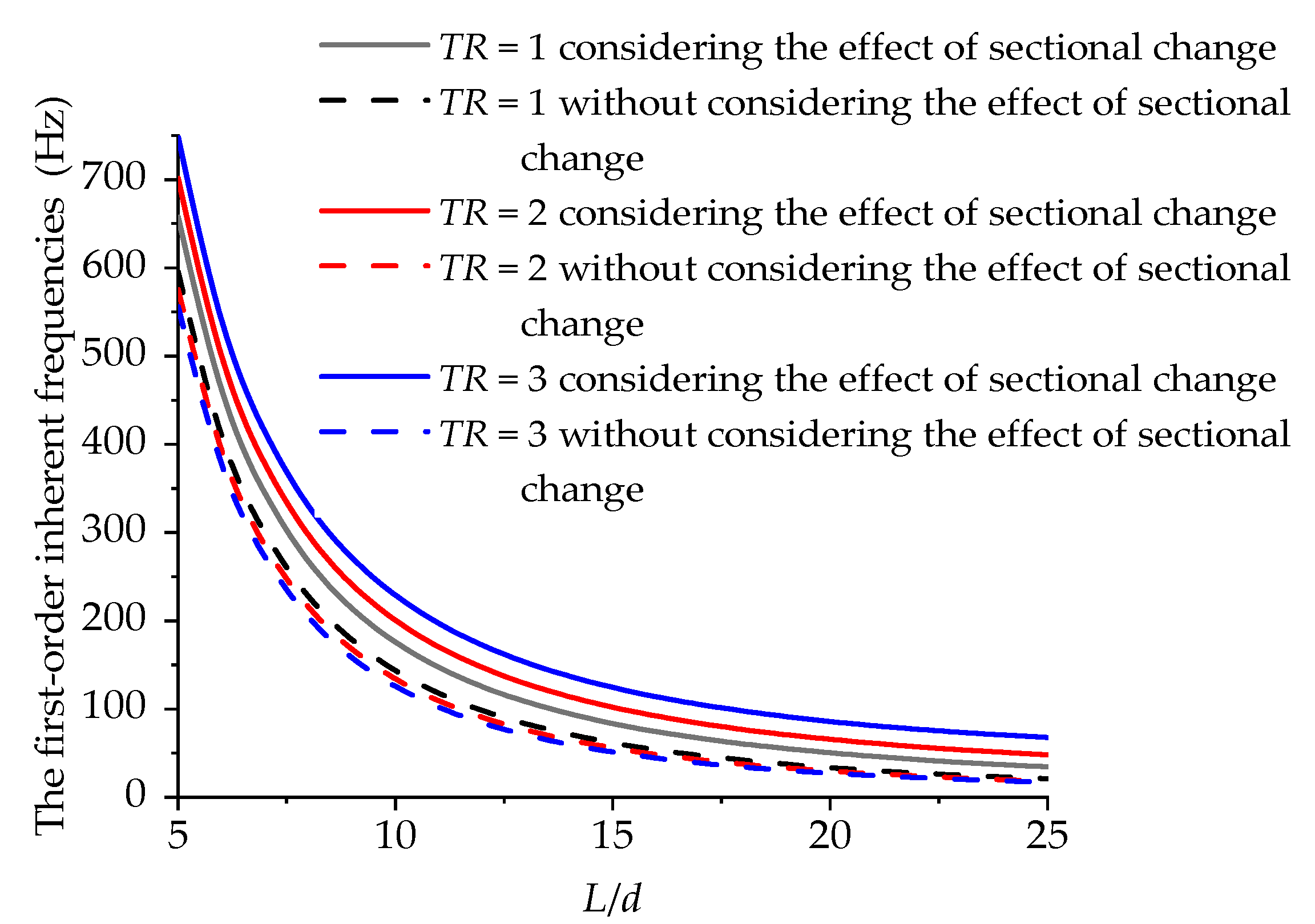
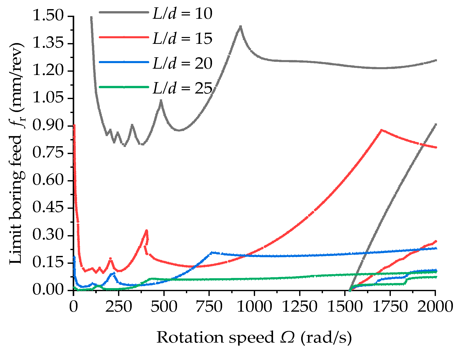
- The increase in the length-to-diameter ratio can reduce the first-order inherent frequency of free vibration and limit the boring feed while imposing no effect on the initiation speed of the new chattering unstable region.
- (2)
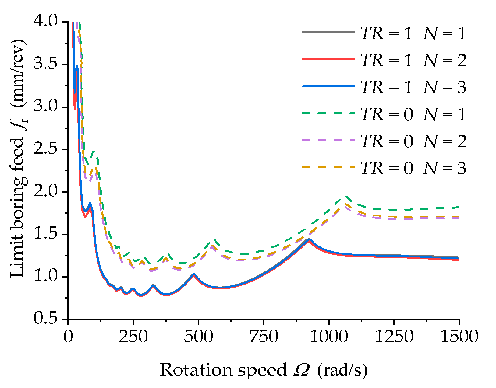
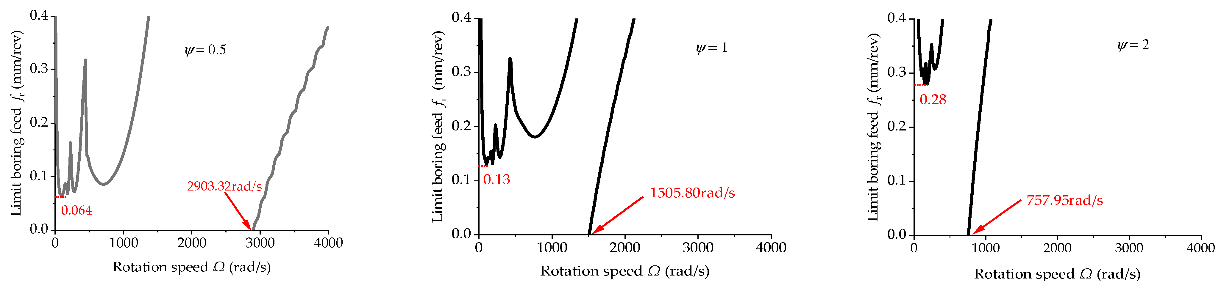
- The increase in the internal damping coefficient can reduce the first-order free vibration inherent frequency of the boring bar and simultaneously enhance the limit boring feed. However, at a high rotation speed, the existence of damping will generate a new boring chattering unstable region. Moreover, the unstable region will appear earlier under a greater damping condition.
- (3)
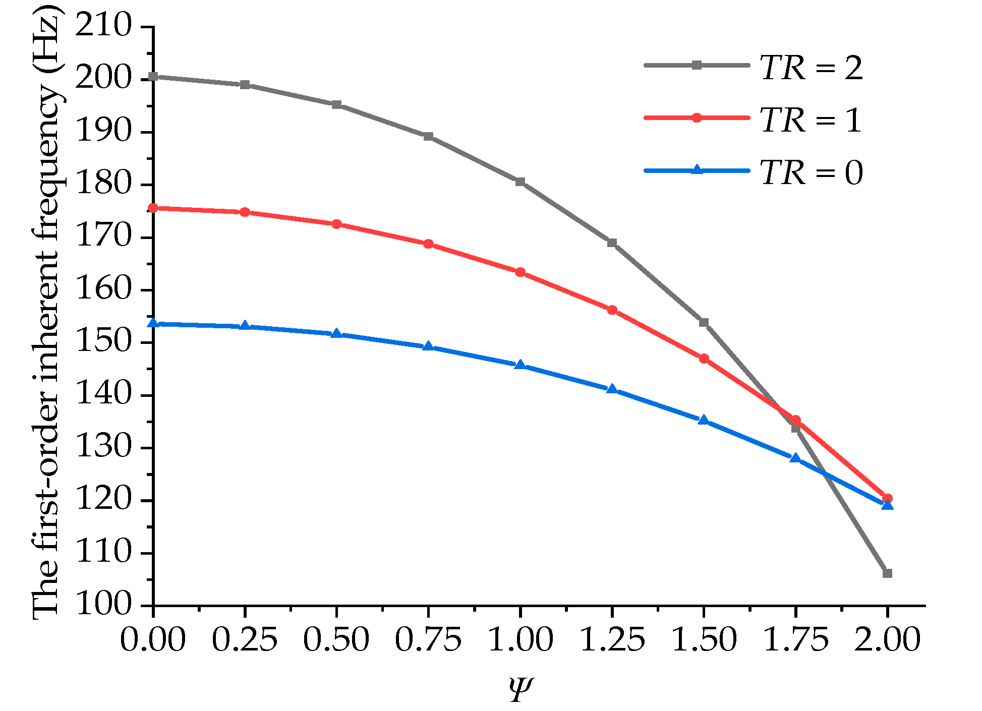
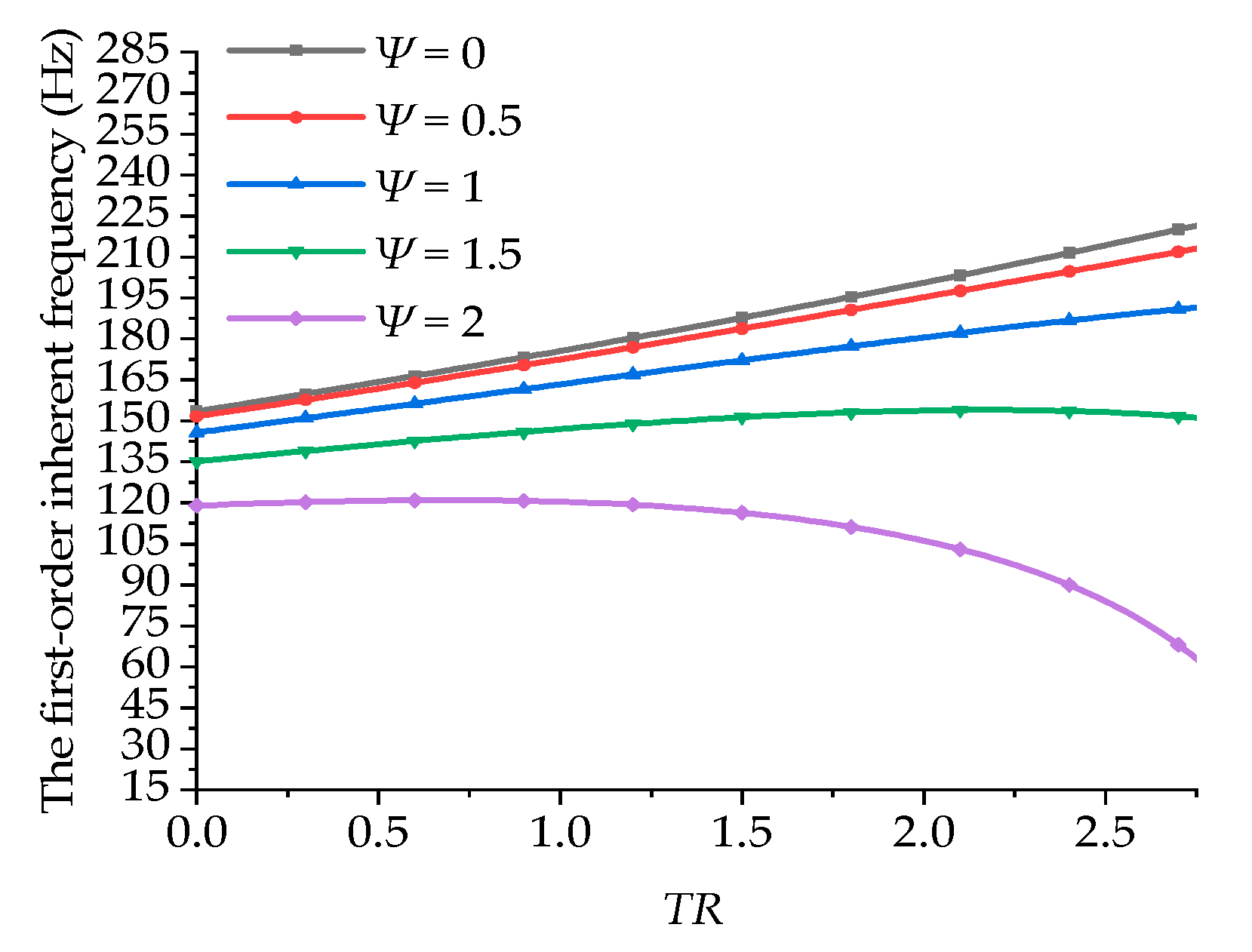
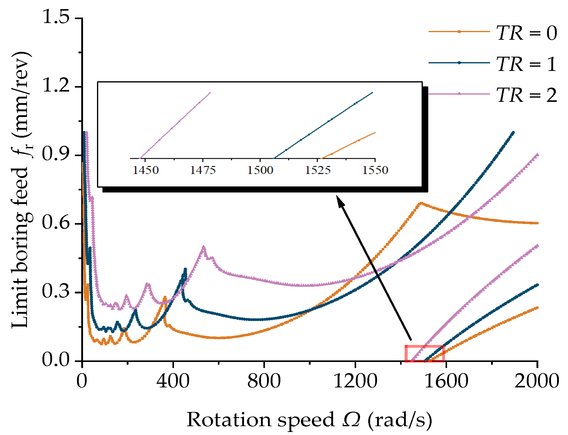
- At a damping ratio of 1 (i.e., ), as the taper ratio of the boring bar increased, the first-order inherent frequency and the limit feed during stable boring were enhanced. The taper ratio imposed a slight effect on the initiation speed of the new chattering unstable region during high-speed boring. Meanwhile, both the taper ratio of the boring bar and the damping coefficient had interaction effects on the free vibration characteristics and cutting stability. For the composite variable-section boring bar, the effects of the internal damping and taper ratio should be considered. This is an innovative point in this study.
- (4)
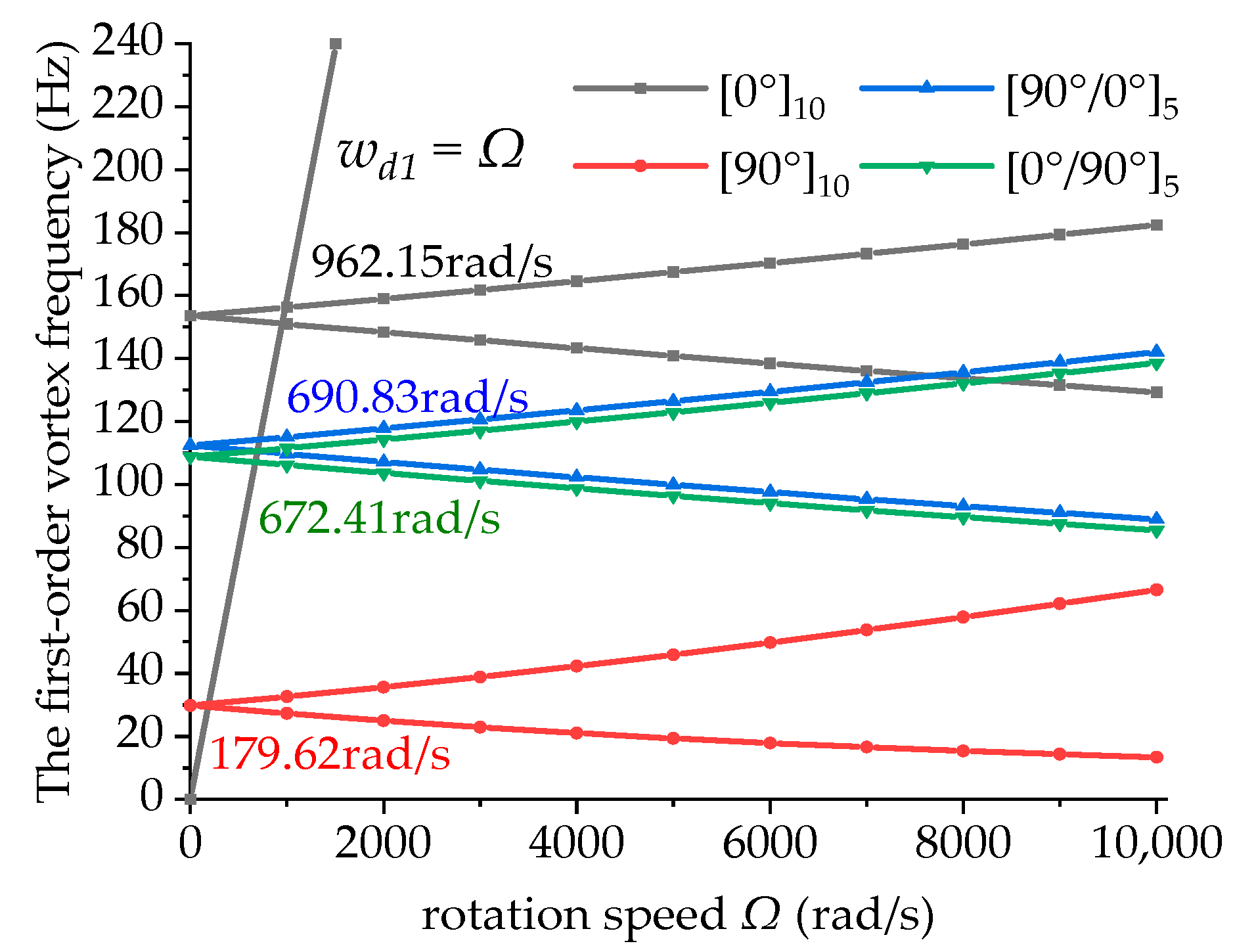
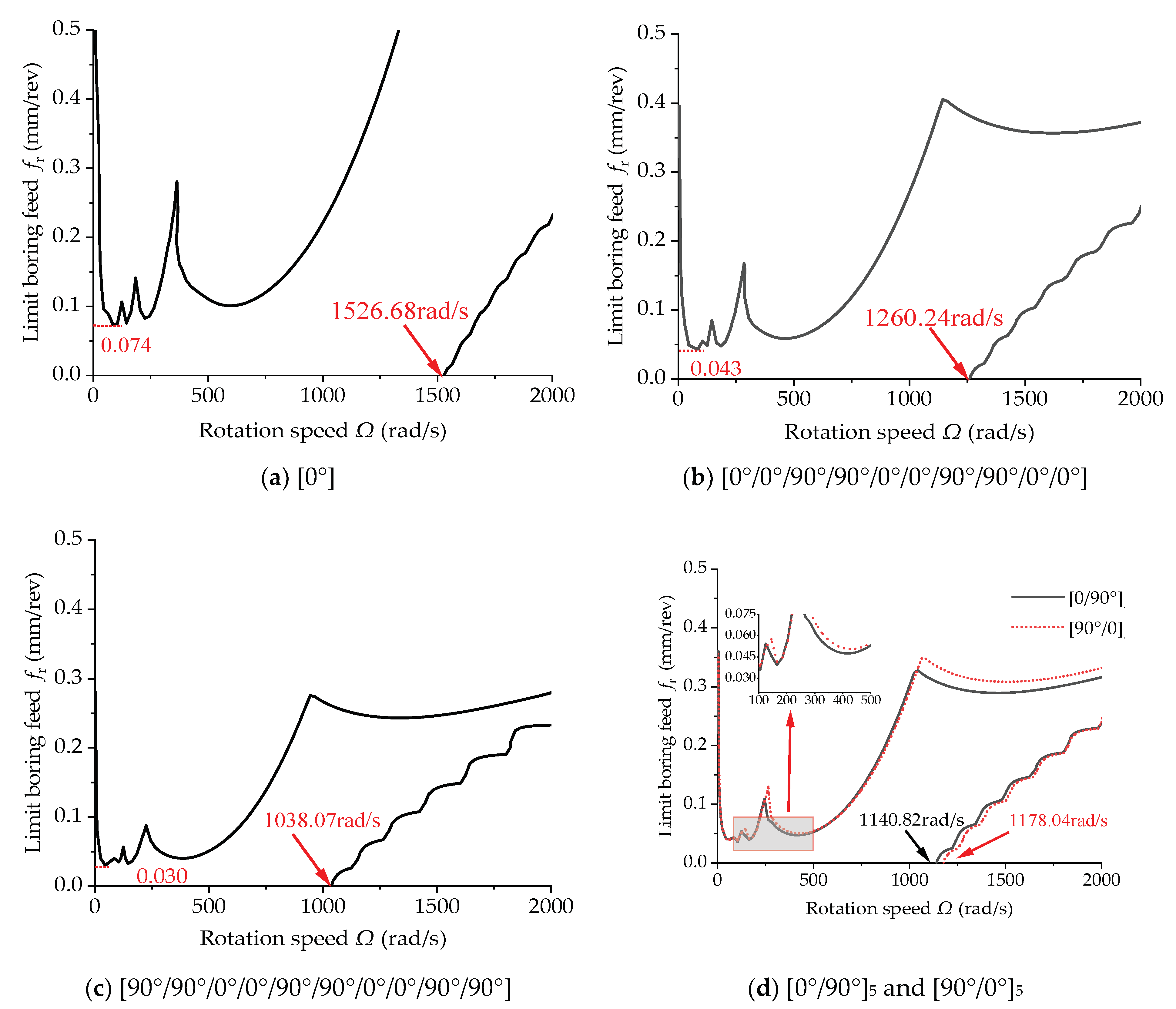
- The ply angle can significantly affect the stable region during the boring process. When the ply angle was 0°, the stable region achieved the maximum, accompanied by large rigidity and small damping. Therefore, the external surface should adopt a 0° ply mode to enhance the cutting stability.
Author Contributions
Funding
Conflicts of Interest
Appendix A
References
- Hao, C.; Zhen, D.; Bing, Z.Z.; Shuai, C. Design of a new type of deep hole boring device. J. Phys. Conf. Ser. 2021, 1748, 062038. [Google Scholar]
- Sino, R.; Baranger, T.N.; Chatelet, E.; Jacquet, G. Dynamic analysis of a rotating composite shaft. Compos. Sci. Technol. 2008, 68, 337–345. [Google Scholar] [CrossRef] [Green Version]
- Moetakef-Imani, B.; Yussefian, N. Dynamic simulation of boring process. Int. J. Mach. Tool Manuf. 2009, 49, 1096–1103. [Google Scholar] [CrossRef]
- Merritt, H.E. Theory of self-excited machine-tool chatter: Contribution to machine-tool chatter research—1. J. Eng. Ind. 1965, 87, 447–454. [Google Scholar] [CrossRef]
- Insperger, T.; Stepan, G. Act-and-wait control concept for discrete-time systems with feedback delay. IET Control. Theory Appl. 2007, 1, 553–557. [Google Scholar] [CrossRef] [Green Version]
- Altintas, Y.; Weck, M. Chatter Stability of Metal Cutting and Grinding. CIRP Ann. Manuf. Technol. 2004, 53, 619–642. [Google Scholar] [CrossRef]
- Solis, E.; Peres, C.R.; Jiménez, J.E.; Alique, J.R.; Monje, J.C. A new analytical–experimental method for the identification of stability lobes in high-speed milling. Int. J. Mach. Tool Manuf. 2004, 44, 1591–1597. [Google Scholar] [CrossRef]
- Li, M.; Zhang, G.; Yu, H. Complete discretization scheme for milling stability prediction. Nonlinear Dyn. 2013, 71, 187–199. [Google Scholar] [CrossRef]
- Zhou, X.; Yu, D.; Shao, X.; Zhang, S.; Wang, S. Research and applications of viscoelastic vibration damping materials: A review. Compos. Struct. 2016, 136, 460–480. [Google Scholar] [CrossRef]
- Treviso, A.; van Genechten, B.; Mundo, D.; Tournour, M. Damping in composite materials: Properties and models. Compos. Part B 2015, 78, 144–152. [Google Scholar] [CrossRef]
- Mendonça, W.R.D.P.; de Medeiros, E.C.; Pereira, A.L.R.; Mathias, M.H. The dynamic analysis of rotors mounted on composite shafts with internal damping. Compos. Struct. 2017, 167, 50–62. [Google Scholar] [CrossRef] [Green Version]
- Montagnier, O.; Hochard, C. Dynamics of a supercritical composite shaft mounted on viscoelastic supports. J. Sound Vib. 2014, 333, 470–484. [Google Scholar] [CrossRef] [Green Version]
- Denghui, L.; Hongrui, C.; Xuefeng, C. Active control of milling chatter considering the coupling effect of spindle-tool and workpiece systems. Mech. Syst. Signal Process. 2022, 169, 108769. [Google Scholar]
- Molnar, G.T.; Insperger, T.; Hogan, J.S.; Stepan, G. Estimation of the Bistable Zone for Machining Operations for the Case of a Distributed Cutting-Force Model. J. Comput. Nonlinear Dyn. 2016, 11, 51008. [Google Scholar] [CrossRef] [Green Version]
- Qinliang, L.; Bo, W.; Bin, Z.; Bangchun, W. Research on the Chatter Stability of Machine System Taking the Nonlinear Hysteretic Force into Consi. Chin. J. Mech. Eng. 2013, 49, 43–49. [Google Scholar]
- Kim, W. Vibration of a Rotating Tapered Composite Shaft and Applications to High Speed Cutting; University of Michigan: Ann Arbor, MI, USA, 1999. [Google Scholar]
- Tian, J.; Hutton, S.G. Chatter instability in milling systems with flexible rotating spindles—A new theoretical approach. J. Manuf. Sci. Eng. 2001, 123, 1–9. [Google Scholar] [CrossRef]
- Jingmin, M.; Yongsheng, R. Free vibration and chatter stability of a rotating thin-walled composite bar. Adv. Mech. Eng 2018, 10, 1687814018798265. [Google Scholar]
- Jingmin, M.; Jianfeng, X.; Yongsheng, R. Analysis on free vibration and stability of rotating composite milling bar with large aspect ratio. Appl. Sci. 2020, 10, 3557–3573. [Google Scholar]
- Kapoor, S.G.; Zhang, G.M.; Bahney, L.L. Stability analysis of the boring process system. Manuf. Eng. Trans. 1984, 454–459. [Google Scholar]
- Subramani, G.; Kapoor, S.G.; Devor, R.E. A model for the prediction of bore cylindricity during machining. J. Eng. Ind. 1993, 115, 15–22. [Google Scholar] [CrossRef]
- Kim, W.; Argento, A.; Scott, R.A. Forced vibration and dynamic stability of a rotating tapered composite timoshenko shaft: Bending motions in end-milling operations. JSV 2001, 246, 583–600. [Google Scholar] [CrossRef]
- Smith, S.; Tlusty, J. An overview of modeling and simulation of the milling process. J. Eng. Ind. 1991, 113, 169–175. [Google Scholar] [CrossRef]


| Graphite Epoxy | Steel | |
|---|---|---|
| E1 (GPa) | 192 | 207 |
| E2 = E3 (GPa) | 7.24 | 207 |
| G12 = G13 (GPa) | 4.07 | 80 |
| G23 (GPa) | 3 | 80 |
| v12 = v13 | 0.24 | 0.2975 |
| ρ (kg/m3) | 1610 | 7700 |
| Taper Ratio of the Boring Bar | Length-to-Diameter Ratio | First-Order Inherent Frequency (Hz) | ||
|---|---|---|---|---|
| Simulation Results of the ANSYS Model (AR) | The Established Model Considering the Sectional Change and the Errors Compared with the AR Simulation Results | The Established Model without Considering the Sectional Change and the Errors Compared with the AR Simulation Results | ||
| TR = 1 | 10 | 163.24 | 175.62 7.58% | 143.51 −12.09% |
| 12 | 123.05 | 125.29 1.82% | 98.29 −20.12% | |
| 14 | 96.748 | 94.56 −2.26% | 71.23 −26.38% | |
| TR = 2 | 10 | 180.45 | 200.59 11.16% | 134.11 −25.68 |
| 12 | 138.78 | 146.98 5.91% | 90.68 −34.65% | |
| 14 | 110.83 | 113.93 2.80% | 64.90 −41.44 | |
| Number of Vibration Mode Functions | 1 | 2 | 3 |
|---|---|---|---|
| Limit boring feed when TR = 1 (mm/rev) | 1.149986 | 1.074399 | 1.091239 |
| Limit boring feed when TR = 0 (mm/rev) | 0.790758 | 0.776207 | 0.787462 |
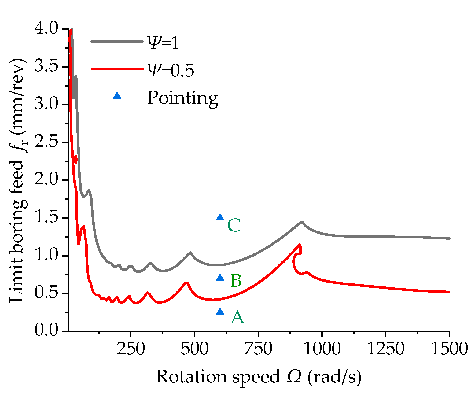
| Point | Rotation Speed (rad/s) | Feed (mm/rev) |
|---|---|---|
| A | 600 | 0.25 |
| B | 600 | 0.75 |
| C | 600 | 1.5 |
Publisher’s Note: MDPI stays neutral with regard to jurisdictional claims in published maps and institutional affiliations. |
© 2022 by the authors. Licensee MDPI, Basel, Switzerland. This article is an open access article distributed under the terms and conditions of the Creative Commons Attribution (CC BY) license (https://creativecommons.org/licenses/by/4.0/).
Share and Cite
Ma, J.; Xu, J.; Li, L.; Liu, X.; Gao, M. Analysis of Cutting Stability of a Composite Variable-Section Boring Bar with a Large Length-to-Diameter Ratio Considering Internal Damping. Materials 2022, 15, 5465. https://0-doi-org.brum.beds.ac.uk/10.3390/ma15155465
Ma J, Xu J, Li L, Liu X, Gao M. Analysis of Cutting Stability of a Composite Variable-Section Boring Bar with a Large Length-to-Diameter Ratio Considering Internal Damping. Materials. 2022; 15(15):5465. https://0-doi-org.brum.beds.ac.uk/10.3390/ma15155465
Chicago/Turabian StyleMa, Jingmin, Jianfeng Xu, Longfei Li, Xingguang Liu, and Ming Gao. 2022. "Analysis of Cutting Stability of a Composite Variable-Section Boring Bar with a Large Length-to-Diameter Ratio Considering Internal Damping" Materials 15, no. 15: 5465. https://0-doi-org.brum.beds.ac.uk/10.3390/ma15155465