
An Approximate Method for Calculating Elastic–Plastic Stress and Strain on Notched Specimens

 ,
,  ,
,
Abstract
:1. Introduction
2. Materials and Methods
2.1. Approximate Method
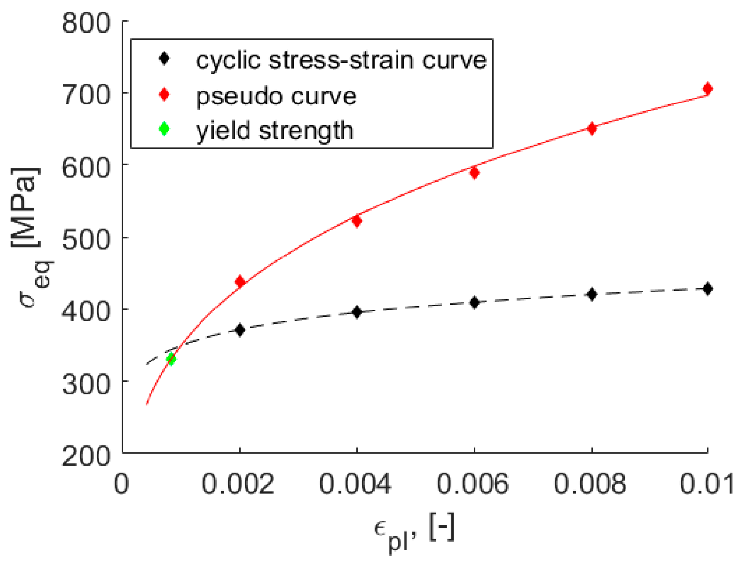
2.1.1. Establishing Pseudostress Material Curve
2.1.2. Getting Real Strain and Real Stress
2.1.3. Equivalence of Pseudo and Real Plastic Strain Tensors
2.1.4. Approximation Method Step by Step
- Pseudomaterial curve is established.
- Pseudostress history is obtained either by elastic FEA or using stress concentration factors [10].
- The plasticity model is applied to the pseudostress history. In this step, plasticity parameters Ci and γi obtained for the pseudomaterial are used. The plastic strain tensor and the accumulated strain are calculated.
- The plasticity model is applied to the plastic strain tensor obtained and to the accumulated strain. In this step, the plasticity parameters Ci and γi for the real material are used. Real stress and real backstress are calculated.
2.2. Abdel–Karim–Ohno Plasticity Model
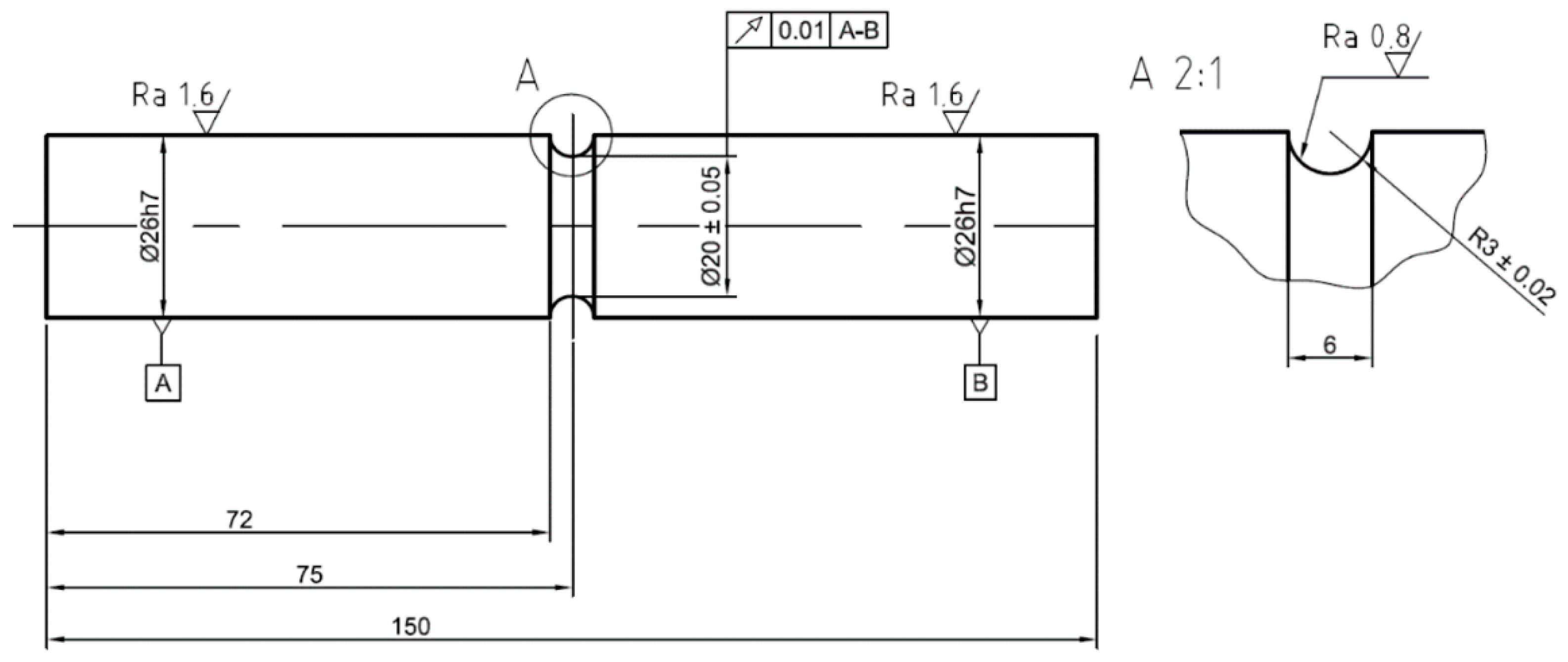
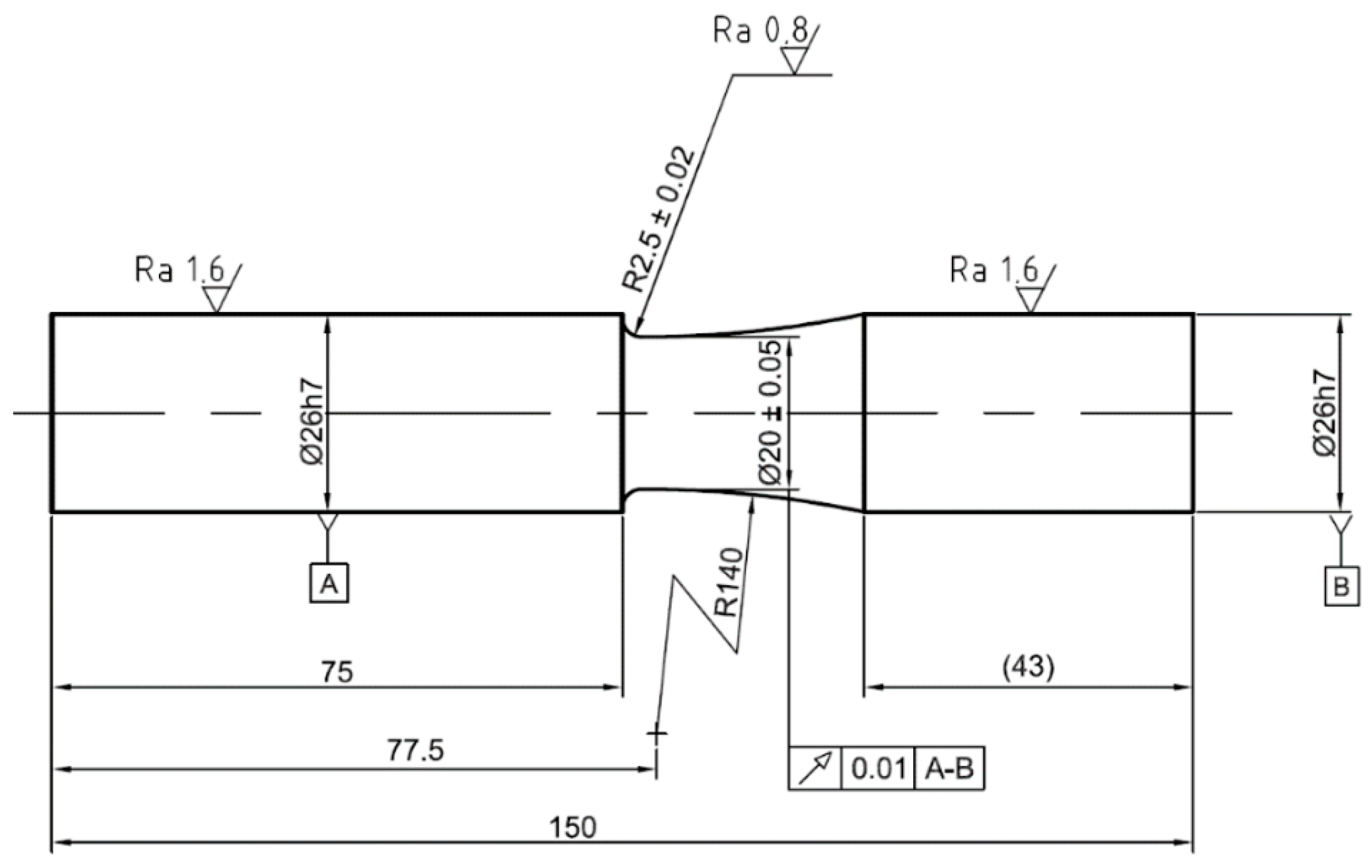
2.3. Experimental Data
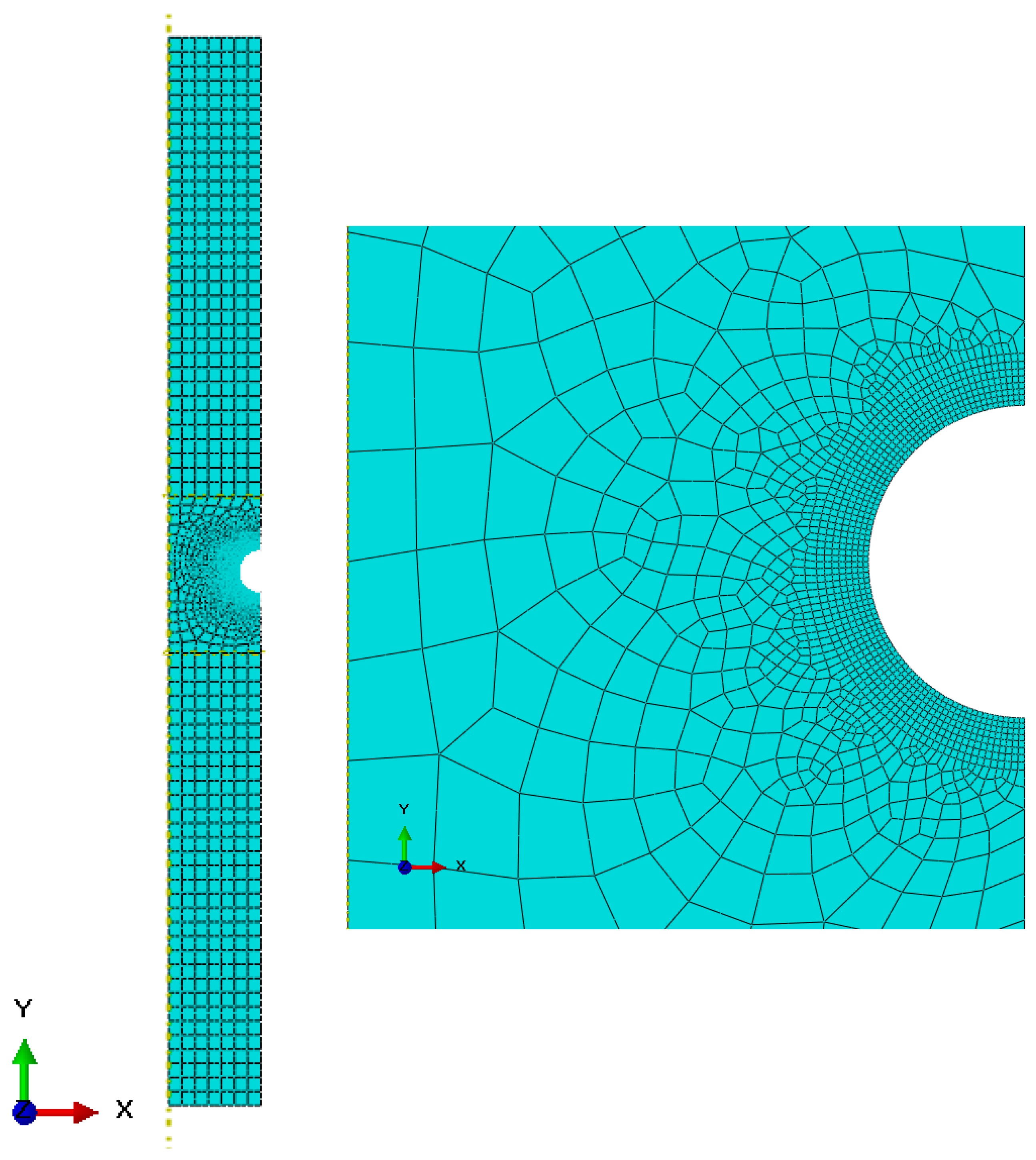
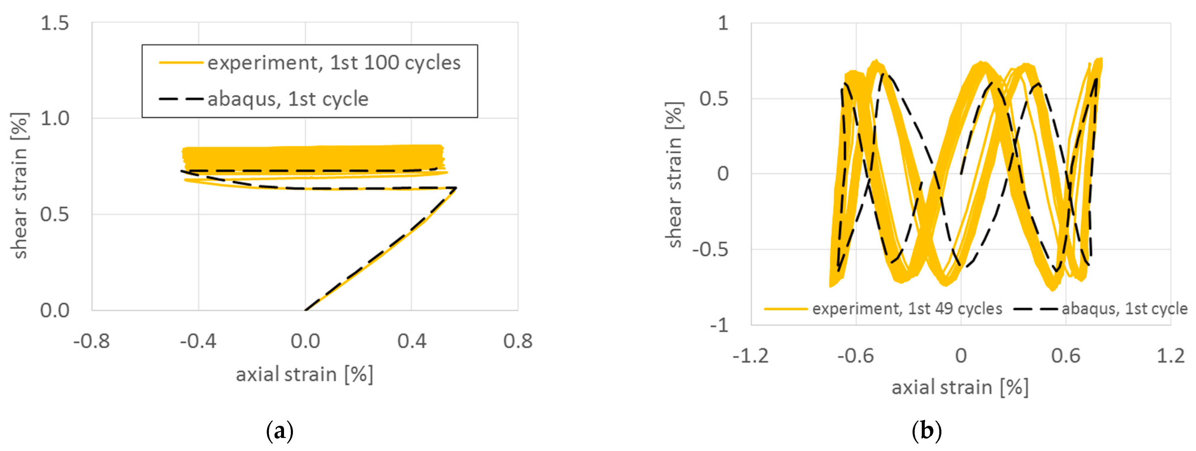
3. Finite Element Analyses
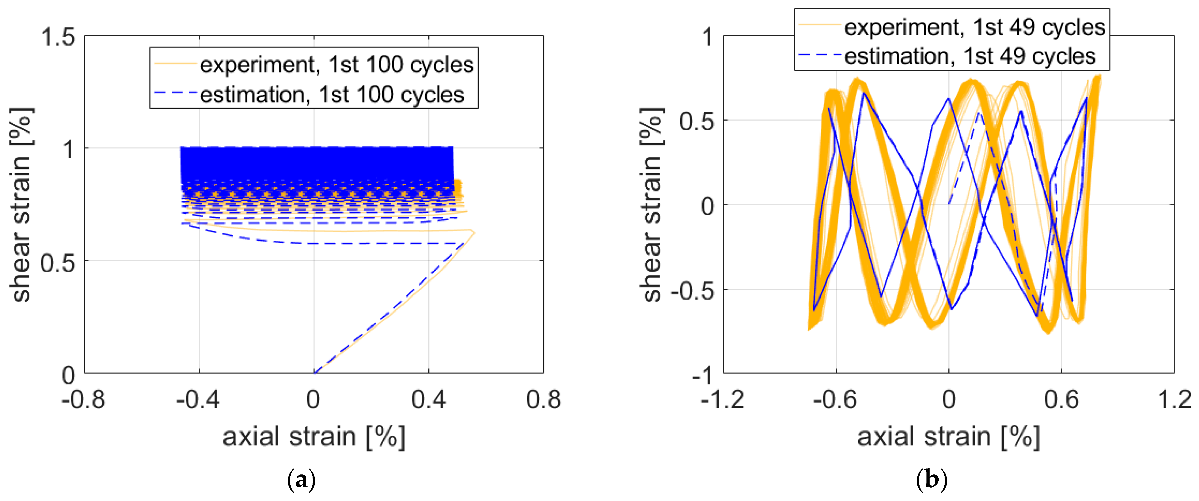
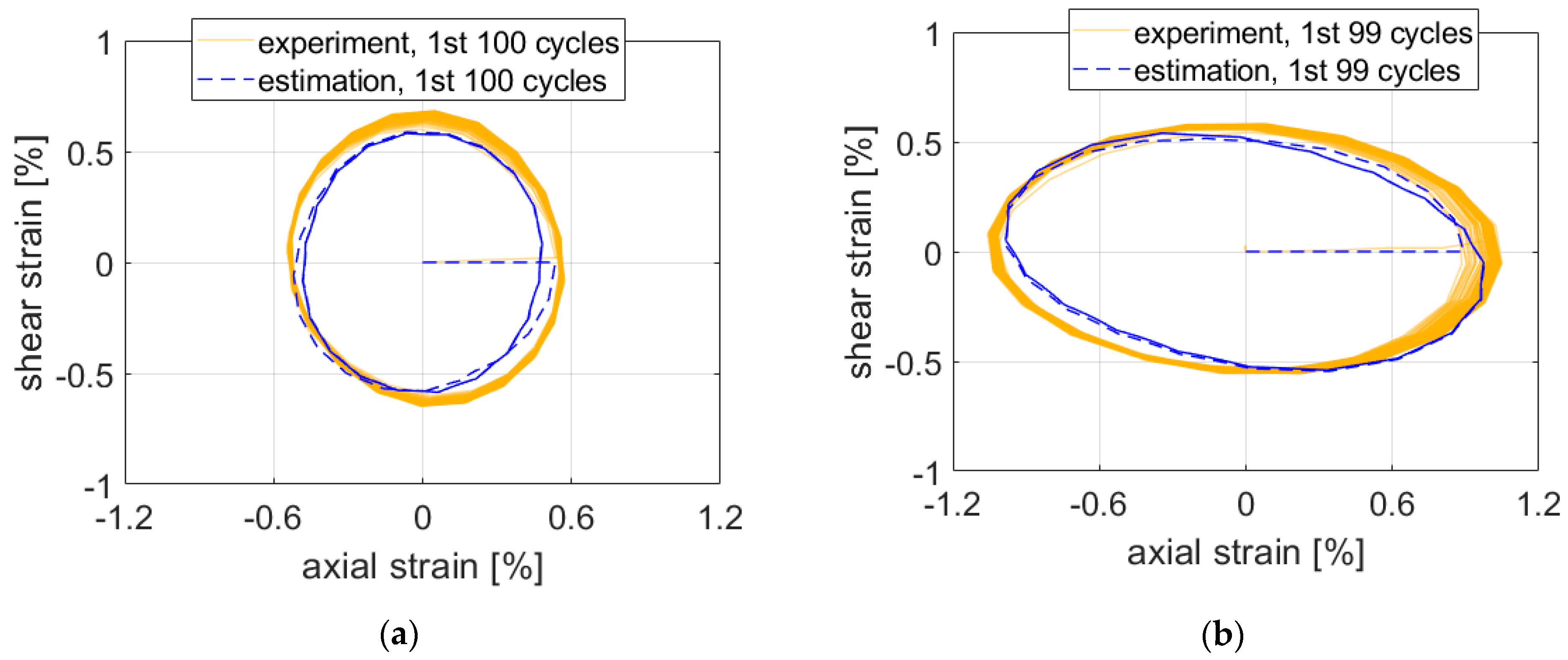
4. Implementation of Approximation Method
5. Results and Discussion
6. Conclusions
Author Contributions
Funding
Institutional Review Board Statement
Informed Consent Statement
Data Availability Statement
Conflicts of Interest
Appendix A. Implementation of Approximate Method in MATLAB
References
- Hoffmann, M.; Seeger, T. Estimating Multiaxial Elastic-Plastic Notch Stresses and Strains in Combined Loading. Biaxial Multiaxial Fatigue 1989, 3–24. Available online: https://pdfcoffee.com/estimating-multiaxial-elastic-plastic-notch-stresses-and-strains-in-combined-loading-pdf-pdf-free.html (accessed on 29 December 2021).
- Moftakhar, A.; Buczynski, A.; Glinka, G. Calculation of elasto-plastic strains and stresses in notches under multiaxial loading. Int. J. Fatigue 1995, 70, 357–373. [Google Scholar] [CrossRef]
- Singh, M.N.K.; Glinka, G.; Dubey, R.N. Elastic-plastic stress-strain calculation in notched bodies subjected to non-proportional loading. Int. J. Fract 1996, 76, 39–60. [Google Scholar] [CrossRef]
- Buczynski, A.; Glinka, G. Elastic-plastic stress-strain analysis of notches under non-proportional loading. In Proceedings of the 5th International Conference on Biaxial/Multiaxial Fatigue and Fracture, Cracow, Poland, 8–12 September 1997; pp. 461–479. [Google Scholar]
- Reinhardt, W.; Moftakhar, A.; Glinka, G. An Efficient Method for Calculating Multiaxial Elasto-Plastic Notch Tip Strains and Stresses under Proportional Loading. Fatigue Fract. Mech. 1997, 27, 613–629. [Google Scholar]
- Lutovinov, M.; Černý, J.; Papuga, J. A comparison of methods for calculating notch tip strains and stresses under multiaxial loading. Frat. Integrita Strutt. 2016, 38, 237–243. [Google Scholar] [CrossRef]
- Barkey, M.E. Calculation of Notch Strains under Multiaxial Nominal Loading. Ph.D. Thesis, University of Illinois, Champaign, IL, USA, 1993. [Google Scholar]
- Koettgen, V.B.; Barkey, M.E.; Socie, D.F. Pseudo stress and pseudo strain based approaches to multiaxial notch analysis. Fatigue Fract. Eng. Mater. Struct. 1995, 18, 981–1006. [Google Scholar] [CrossRef]
- Langlais, T.E. Computational Methods for Multiaxial Fatigue Analysis. Ph.D. Thesis, University of Minnesota, Minneapolis, MN, USA, 1999. [Google Scholar]
- Firat, M. A notch strain calculation of a notched specimen under axial-torsion loadings. Mater. Des. 2011, 32, 3876–3882. [Google Scholar] [CrossRef]
- Ince, A.; Buczynski, A.; Glinka, G. Computational modeling of multiaxial elasto-plastic stress–strain response for notched components under non-proportional loading. Int. J. Fatigue 2014, 62, 42–52. [Google Scholar] [CrossRef]
- Ye, D.; Hertel, O.; Vormwald, M. A unified expression of elastic–plastic notch stress–strain calculation in bodies subjected to multiaxial cyclic loading. Int. J. Solids Struct. 2008, 45, 6177–6189. [Google Scholar] [CrossRef] [Green Version]
- Li, J.; Zhang, Z.; Li, C. A coupled Armstrong-Frederick type plasticity correction methodology for calculating multiaxial notch stresses and strains. J. Fail. Anal. Prev. 2017, 17, 706–716. [Google Scholar] [CrossRef]
- Tao, Z.-Q.; Shang, D.-G.; Sun, Y.-J. New pseudo stress correction method for estimating local strains at notch under multiaxial cyclic loading. Int. J. Fatigue 2017, 103, 280–293. [Google Scholar] [CrossRef]
- Li, D.-H.; Shang, D.-G.; Xue, L.; Li, L.-J.; Wang, L.-W.; Cui, J. Notch stress-strain estimation method based on pseudo stress correction under multiaxial thermo-mechanical cyclic loading. Int. J. Solids Struct. 2020, 199, 144–157. [Google Scholar] [CrossRef]
- Kraft, J.; Vormwald, M. Energy driven integration of incremental notch stress-strain approximation for multiaxial cyclic loading. Int. J. Fatigue 2021, 145, 106043. [Google Scholar] [CrossRef]
- Mróz, Z. On the description of anisotropic work hardening. J. Mech. Phys. Solids 1967, 15, 163–175. [Google Scholar] [CrossRef]
- Chu, C.-C. A three-dimensional model of anisotropic hardening in metals and its application to the analysis of sheet metal forming. J. Mech. Phys. Solids 1984, 32, 197–212. [Google Scholar] [CrossRef]
- Chaboche, J.L. Constitutive equations for cyclic plasticity and cyclic viscoplasticity. Int. J. Plast. 1989, 5, 247–302. [Google Scholar] [CrossRef]
- Prandtl, W. Spannungsverteilung in plastischen kerpern. In Proceedings of the First International Congress on Applied Mechanics, Delft, The Netherlands, 22–26 April 1924. [Google Scholar]
- Reuss, E. Beruecksichtigung der elastischen Formaenderungen. ZAMM 1930, 10, 266–274. [Google Scholar] [CrossRef]
- Garud, Y.S. A new approach to the evaluation of fatigue under multiaxial loadings. J. Eng. Mater. T ASME 1981, 103, 118–125. [Google Scholar] [CrossRef]
- Glinka, G.; Roostaei, A.A.; Jahed, H. Cyclic plasticity applied to the notch analysis of metals. In Cyclic Plasticity of Metals: Modeling Fundamentals and Applications; Motlagh, H.J., Roostaei, A.A., Eds.; Elsevier: Amsterdam, The Netherlands, 2022; pp. 283–323. [Google Scholar] [CrossRef]
- Jiang, Y.; Sehitoglu, H. Modeling of cyclic ratchetting plasticity, part I: Development of constitutive relations. J. Appl. Mech. 1996, 63, 720–725. [Google Scholar] [CrossRef]
- Nagode, M.; Hack, M.; Fajdiga, M. Low cycle thermo-mechanical fatigue: Damage operator approach. Fatigue Fract. Eng. Mater. Struct. 2010, 33, 149–160. [Google Scholar] [CrossRef]
- Ohno, N.; Wang, J.D. Kinematic hardening rules with critical state of dynamic recovery, part I: Formulation and basic features for ratchetting behavior. Int. J. Plast 1993, 9, 375–390. [Google Scholar] [CrossRef]
- Abdel-Karim, M.; Ohno, N. Kinematic hardening model suitable for ratcheting with steady-state. Int. J. Plast 2000, 16, 225–240. [Google Scholar] [CrossRef]
- Halama, R.; Markopoulos, A.; Šmach, J.; Govindaraj, B. Theory, application and implementation of modified Abdel-Karim-Ohno model for uniaxial and multiaxial fatigue loading. In Fatigue Damage in Metals—Numerical Based Approaches and Applications; Cernescu, A., Ed.; Elsevier: Amsterdam, The Netherlands, 2022; submitted. [Google Scholar]
- Chaboche, J.L.; Dang Van, K.; Cordier, G. Modelization of the strain memory effect on the cyclic hardening of 316 stainless steel. In Proceedings of the 5th International Conference on Structural Mechanics in Reactor Technology, Division L11/3, Berlin, Germany, 13–17 August 1979; Jaeger, A., Boley, B.A., Eds.; Bundesanstalt főr Materialprőfung: Berlin, Germany, 1979; pp. 1–10. [Google Scholar]
- Armstrong, P.J.; Frederick, C.O. A Mathematical Representation of the Multiaxial Bauschinger Effect; G.E.G.B. Report RD/B/N.; Central Electricity Generating Board and Berkeley Nuclear Laboratories, Research & Development Department: Berkeley, CA, USA, 1966; p. 731. [Google Scholar]
- ASM Aerospace Specification Metals Inc. Available online: http://asm.matweb.com/search/SpecificMaterial.asp?bassnum=MA2124T851 (accessed on 30 December 2021).
- Chen, X.; Jiao, R. Modified kinematic hardening rule for multiaxial ratcheting prediction. Int. J. Plast 2004, 20, 871–898. [Google Scholar] [CrossRef]
- Jiang, Y.; Sehitoglu, H. Cyclic ratcheting of 1070 steel under multiaxial stress states. Int. J. Plast 1994, 10, 579–608. [Google Scholar] [CrossRef]
- WebPlotDigitizer. Web Based Tool to Extract Data from Plots, Images, and Maps. Available online: https://apps.automeris.io/wpd/ (accessed on 30 January 2022).


| Author | Material | Used Data |
|---|---|---|
| Barkey [7] | 1070 steel | [7] |
| Koettgen et al. [8] | steel | only FEA |
| Langlais [9] | 1070 steel | [7] |
| Firat [10] | 1070 steel | [7] |
| Ince et al. [11] | 1070 steel | [7] |
| Ye et al. [12] | S460N steel | [12] |
| Li et al. [13] | 1070 steel, S460N steel | [7,12] |
| Tao et al. [14] | TC21 titanium alloy, 1070 steel | [7,14] |
| Li et al. [15] | GH4169 superalloy | only FEA |
| Kraft [16] | steel | only FEA |
| Real | Pseudo | ||
|---|---|---|---|
| Parameter | Value | Parameter | Value |
| (MPa) | 16,401 | (MPa) | 51,760 |
| (-) | 500 | (-) | 500 |
| (MPa) | 4561 | (MPa) | 7205 |
| (-) | 250 | (-) | 250 |
| (MPa) | 1948 | (MPa) | 3908 |
| (-) | 166.7 | (-) | 166.7 |
| (MPa) | 1097 | (MPa) | 2637 |
| (-) | 125 | (-) | 125 |
| (MPa) | 4216 | (MPa) | 27,589 |
| (-) | 100 | (-) | 100 |
| Stress (MPa) | Plastic Strain (-) |
|---|---|
| 330 | 0.000 |
| 371.56 | 0.002 |
| 395.19 | 0.004 |
| 409.72 | 0.006 |
| 420.35 | 0.008 |
| 428.78 | 0.010 |
| 435.79 | 0.012 |
| 441.81 | 0.014 |
| 447.09 | 0.016 |
| 451.81 | 0.018 |
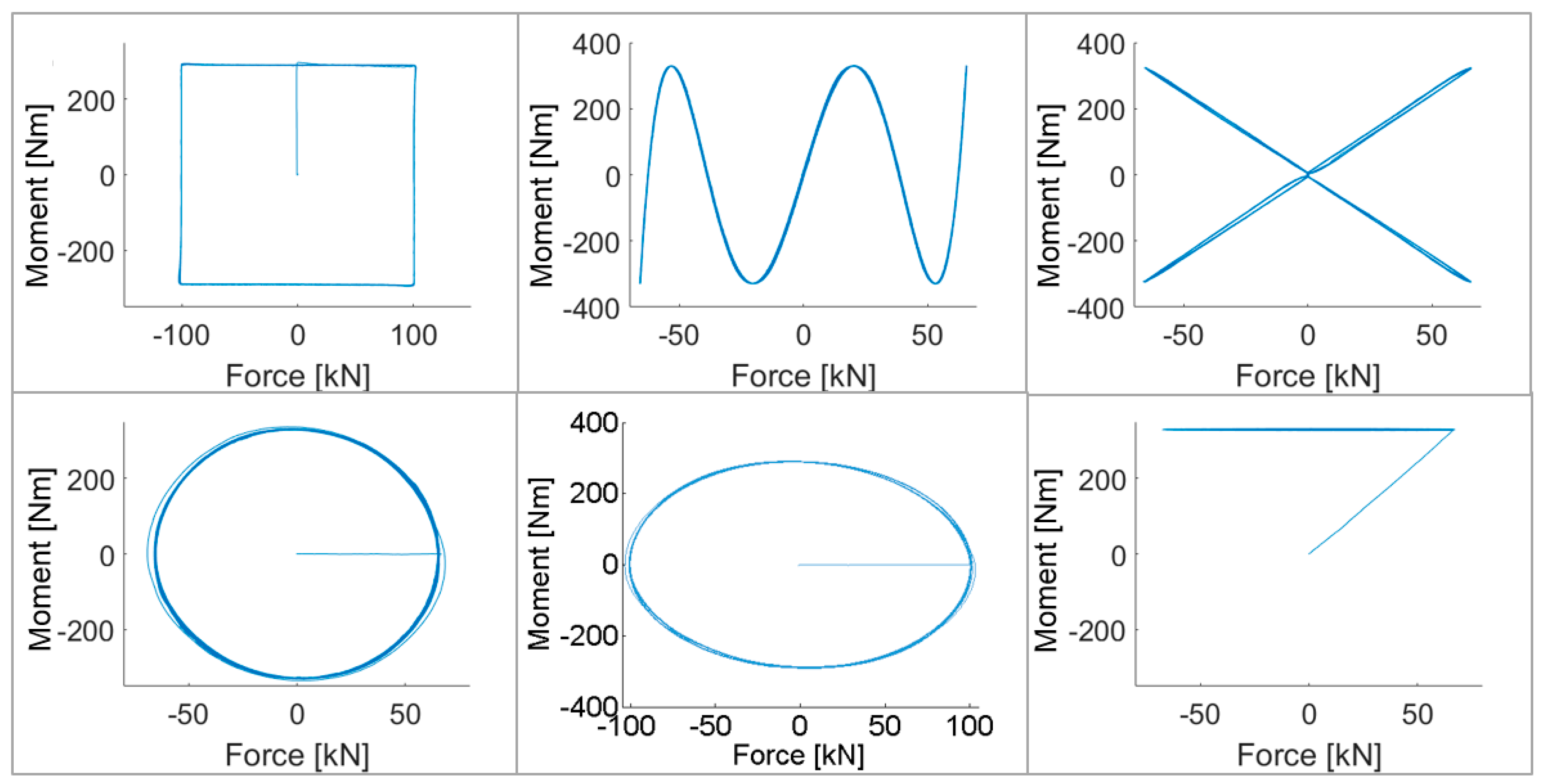
| Material | Stress Concentration Factors | Loading Path | Nominal Axial Stress S22 (MPa) | Nominal Shear Stress S23 (MPa) | ||
|---|---|---|---|---|---|---|
| Tension Kt22 | Torsion Kt23 | Transverse Kt33 | ||||
| 1070 steel [7] | 1.31 | 1.53 | 0.27 | NV | 258 | 168 |
| square | 296 | 193 | ||||
| TC21 titanium alloy [14] | 1.45 | 1.17 | 0.3 | NV | 299 | 173 |
| rotated V | 299 | 173 | ||||
| Material | Young’s Modulus | Poisson’s Ratio | Ramberg–Osgood Parameters | Cyclic Yield Strength | Ratcheting Parameter | |
|---|---|---|---|---|---|---|
| (GPa) | (-) | K (MPa) | n (-) | (MPa) | μi (-) | |
| 1070 steel [7] | 210 | 0.3 | 1736 | 0.199 | 286 | 0.3 |
| TC21 titanium alloy [14] | 121 | 0.3 | 1558 | 0.093 | 400 | 0.1 |
| Material | Path | Strain Component | RE of Proposed Model (%) | RE of Estimate in [14] (%) |
|---|---|---|---|---|
| 1070 steel | NV | Axial | 4.26 | −5.29 |
| Shear | 7.28 | −2.85 | ||
| Square | Axial | −4.74 | −4.98 | |
| Shear | −13.36 | −14.71 | ||
| TC21 titanium alloy | NV | Axial | 5.91 | −6.76 |
| Shear | −0.35 | −5.64 | ||
| Rotated V | Axial | 13.53 | −3.83 | |
| Shear | 8.20 | −3.32 |
Publisher’s Note: MDPI stays neutral with regard to jurisdictional claims in published maps and institutional affiliations. |
© 2022 by the authors. Licensee MDPI, Basel, Switzerland. This article is an open access article distributed under the terms and conditions of the Creative Commons Attribution (CC BY) license (https://creativecommons.org/licenses/by/4.0/).
Share and Cite
Lutovinov, M.; Halama, R.; Papuga, J.; Bartošák, M.; Kuželka, J.; Růžička, M. An Approximate Method for Calculating Elastic–Plastic Stress and Strain on Notched Specimens. Materials 2022, 15, 1432. https://0-doi-org.brum.beds.ac.uk/10.3390/ma15041432
Lutovinov M, Halama R, Papuga J, Bartošák M, Kuželka J, Růžička M. An Approximate Method for Calculating Elastic–Plastic Stress and Strain on Notched Specimens. Materials. 2022; 15(4):1432. https://0-doi-org.brum.beds.ac.uk/10.3390/ma15041432
Chicago/Turabian StyleLutovinov, Maxim, Radim Halama, Jan Papuga, Michal Bartošák, Jiří Kuželka, and Milan Růžička. 2022. "An Approximate Method for Calculating Elastic–Plastic Stress and Strain on Notched Specimens" Materials 15, no. 4: 1432. https://0-doi-org.brum.beds.ac.uk/10.3390/ma15041432