Multi-Objective Bi-Level Programming for the Energy-Aware Integration of Flexible Job Shop Scheduling and Multi-Row Layout

School of Management Science and Engineering, Anhui University of Technology, Ma’anshan 243032, China
*
Author to whom correspondence should be addressed.
Algorithms 2018, 11(12), 210; https://0-doi-org.brum.beds.ac.uk/10.3390/a11120210
Submission received: 23 November 2018
/
Revised: 13 December 2018
/
Accepted: 13 December 2018
/
Published: 17 December 2018
(This article belongs to the Special Issue Algorithms for Decision Making)
Abstract
:The flexible job shop scheduling problem (FJSSP) and multi-row workshop layout problem (MRWLP) are two major focuses in sustainable manufacturing processes. There is a close interaction between them since the FJSSP provides the material handling information to guide the optimization of the MRWLP, and the layout scheme affects the effect of the scheduling scheme by the transportation time of jobs. However, in traditional methods, they are regarded as separate tasks performed sequentially, which ignores the interaction. Therefore, developing effective methods to deal with the multi-objective energy-aware integration of the FJSSP and MRWLP (MEIFM) problem in a sustainable manufacturing system is becoming more and more important. Based on the interaction between FJSSP and MRWLP, the MEIFM problem can be formulated as a multi-objective bi-level programming (MOBLP) model. The upper-level model for FJSSP is employed to minimize the makespan and total energy consumption, while the lower-level model for MRWLP is used to minimize the material handling quantity. Because the MEIFM problem is denoted as a mixed integer non-liner programming model, it is difficult to solve it using traditional methods. Thus, this paper proposes an improved multi-objective hierarchical genetic algorithm (IMHGA) to solve this model. Finally, the effectiveness of the method is verified through comparative experiments.
1. Introduction
With the diversification and personalization of market demand, multi-variety and small batch production has been adopted by more and more enterprises, aiming to respond to the changes of customers and provide the market with creative products quickly. Drira et al. [1] reported that, on average, 40% of an enterprise’s sales come from new products. The manufacturing of new products leads to some changes in the process design, processing sequences, and material handling quantity, which has a significant impact on the manufacturing process. Gupta et al. [2] concluded that one-third of USA companies undergo major dislocation of scheduling and layout schemes every two years. As the decision-making focus of the production process, scheduling and layout planning run through the entire manufacturing process. To ensure production efficiency under such a market environment, the scheduling and layout schemes of enterprises must be adaptive to changing demand conditions. In view of this situation, general enterprises tend to re-design scheduling schemes and avoid adjusting layout schemes as much as possible due to time-consuming and expensive re-layout costs. The approach impedes the improvement of enterprises’ responsiveness because the optimization performance of the scheduling scheme strongly depends on the original layout scheme. However, for some labor-intensive enterprises with moderately light machines or workstations that are convenient for re-layout, such as footwear or clothing industries, they can adapt better to the changes of market demand by re-designing the scheduling and layout schemes [3]. It is noted that scheduling determines the allocation of operations to machines and provides detailed material handling information between machines for the optimization of layout, while layout planning determines the optimal positions of all machines in a given workshop according to the specific scheduling scheme. It is observed that there is a close interaction between scheduling and layout planning. Therefore, the coordinated optimization of scheduling and layout planning is of vital importance for enterprises to respond quickly to changes of market demand.
Recently, the issues of environmental protection and energy conservation in manufacturing industries have been gaining more and more attention. Since the beginning of the industrial revolution, the industrial sector has consumed large amounts of energy. Manufacturing enterprises are responsible for approximately 33% of global total energy consumption and 38% of greenhouse gas emissions [4]. Improving the utilization efficiency of resources and energy has become critical for the sustainable development of modern industrial companies [5]. Therefore, the concept of green manufacturing has caused wide concern in academia, society, and industry, referring to reducing pollution and saving energy consumption during the production process. Admittedly, we should improve enterprises’ quick response ability when facing changes of market demand as much as possible, but it cannot be implemented at the expense of the environment. Thus, another goal of enterprises is to determine how to save energy and reduce emissions, without lowering the response ability. It should be noted that a large number of studies [6,7,8,9] have indicated that reasonable scheduling and layout planning for manufacturing systems will save great energy consumption.
Therefore, in order to respond quickly and effectively to changes of market demand and reduce energy consumption, the integrated optimization of scheduling and layout planning is extremely important. However, this integration is still a challenge in both research and applications. In traditional approaches, scheduling and layout planning were carried out sequentially. These approaches cannot consider the scheduling and layout planning problems from the perspective of system optimization and ignore their interaction, which may prevent improvement of the productivity and energy efficiency of the manufacturing system and generate the following problems:
- In much research, scheduling is done based on the assumption that the transportation time between machines is either neglected or determined. However, in the actual workshop, the positions of machines will significantly affect the transportation time of jobs. This may make the enterprises’ production cycle longer or generate production stagnation, which leads to more idle energy consumption. Therefore, the generated scheduling schemes are somehow unrealistic and cannot be readily executed in the workshop, resulting in the optimum scheduling scheme often becoming infeasible;
- After the layout is set, the performance of scheduling schemes is highly dependent on the determined layout scheme. Moreover, if the type and requirement of the product change greatly, the scheduling scheme will change accordingly. As a result, the material handling information between machines will be greatly affected, which may cause the original layout scheme to become inefficient;
- Separate optimization of scheduling and layout planning does not guarantee optimality of the whole manufacturing system since scheduling or layout planning has more than one criterion to be considered, in which many criterions are often conflicting. For example, in the real manufacturing process, each operation could be implemented on a set of machines, including dedicated machines and universal machines. Generally, when an operation is processed on the dedicated machine, the corresponding processing time and energy consumption are minimal. In this manner, the scheduling scheme displays a short completion time and low processing energy consumption, while the corresponding layout scheme may lead to high transportation energy consumption and material handling quantity since the jobs are frequently transported between machines. On the contrary, the scheduling scheme may lead to a long completion time and high processing energy consumption, while the corresponding layout scheme may lead to low transportation energy consumption and material handling quantity. Neither of these manners can obtain a high production efficiency and low energy consumption solution.
The above problems can be conquered by the integration of scheduling and layout planning (ISLP), which has been a hot research topic in recent years. Ranjbar et al. [10] studied a concurrent layout and scheduling problem in a job shop environment to minimize makespan. Ripon et al. [11,12] developed a multi-objective mathematical model for integrated job shop scheduling and the facility layout planning problem that considers makespan, mean flow time, material handling cost, and closeness rating score simultaneously. Mallikarjuna [13] proposed a flexible batch scheduling problem which was integrated with loop layout pattern design, and applied the genetic algorithm (GA) and simulated annealing algorithm (SA) to solve the problem for minimizing makespan and transportation cost. Liu et al. [14] studied an integrated optimization problem of workshop layout and scheduling considering energy consumption to minimize makespan and carbon emission simultaneously, in which they proposed a multi-objective fruit fly optimization algorithm to solve the problem.
Besides this, in the field of cellular manufacturing, Wu et al. [15], Arkat et al. [16], and Fahmy et al. [17] studied the integrated cell formation, group layout, and group scheduling, and applied GA to solve the problem for minimizing makespan. Arkat et al. [18] adopted the multi-objective genetic algorithm (MOGA) for the cell formation problem considering cellular layout and operation scheduling to minimize makespan and transportation cost. Suemitsu et al. [19] proposed a multi-robots cellular manufacturing system layout problem that can determine the positions of manufacturing components and task scheduling simultaneously, and they applied MOGA to solve the problem for minimizing the operation time, layout area, and manipulability.
Although these studies validate that the ISLP can achieve better solutions than the independent optimization method, they still have several disadvantages, as follows:
- (1)
- These studies cannot provide effective guidance for enterprises. Since most of these studies focus on the job shop scheduling problem (JSSP) and discrete workshop layout problem (DWLP), the flexible processing route of jobs and size of machines are neglected, which means that these studies cannot solve more realistic problems, such as the flexible job shop scheduling problem (FJSSP), single-row workshop layout problem (SRWLP), multi-row workshop layout problem (MRWLP), and so on;
- (2)
- The optimality of the layout scheme cannot be ensured. Because most studies of ISLP only consider scheduling objectives, the layout problem is simply appended to the scheduling problem as a constraint, which ignores the interaction between scheduling and layout planning. For the integrated model that only considers scheduling objectives, it is difficult to ensure the feasibility of the scheduling and layout schemes simultaneously. For example, if only the makespan is optimized, a scheduling scheme with lower makespan may be accompanied by an unreasonable layout scheme. The unreasonable layout scheme may result in frequent job delays and processing interruptions, which greatly offsets the economic advantage;
- (3)
- Only a few studies of ISLP consider the energy consumption indicator. If only optimizing the efficiency objectives, a solution with a higher production efficiency may also be a solution with higher energy consumption. The higher energy cost will have an adverse impact on the final profit of enterprises. Admittedly, we should seek a solution that balances energy consumption and production efficiency in solving the ISLP problem.
To overcome these disadvantages, this paper chooses FJSSP and MRWLP, which are more suitable for the real manufacturing system as research objects, and focuses on the interaction between them. Then, the paper proposes a multi-objective energy-aware integration of FJSSP and MRWLP (MEIFM) problem. In the proposed MEIFM, we consider flexible processing routes of jobs and unequal-area machines, as well as the interaction between FJSSP and MRWLP. The interaction is shown in Figure 1. The FJSSP is linked to the MRWLP by the material handling information and distance between machines. The FJSSP’s decision guides the optimization of the layout scheme by material handling information, while the MRWLP’s decision influences the performance of the scheduling scheme by distance between machines. Obviously, the MEIFM can be represented as a Leader-Follower or Stackelberg game, where the FJSSP acts as the leader and the MRWLP acts as the follower. Therefore, the MEIFM is a typical bi-level programming problem.
As both scheduling and layout planning are NP-hard problems [20,21], the MEIFM problem considering the flexible processing route of jobs and unequal-area machines becomes a more complicated problem. Additionally, it is concerned with balancing the production efficiency and energy consumption of the overall manufacturing system, which also makes the problem become more complex. Further, the bi-level programming problem also falls into the class of NP-hard problems [22]. As a result, developing an effective method to deal with the MEIFM problem is a challenge.
To optimize the MEIFM problem, an improved multi-objective hierarchical genetic algorithm (IMHGA) is proposed. The proposed algorithm is designed based on the framework of GA, which is one of the most famous optimization algorithms and has been successfully applied in many bi-level programming problems [23,24,25,26]. Moreover, in the IMHGA, two improved strategies are introduced to enhance the performance of the algorithm based on the characteristics of the problem. One is to design the multi-parent improved precedence operation crossover (MIPOX) and multi-parent multi-point preservative crossover (MMPX) based on the multi-parent crossover method aiming to enhance the global searching ability of the algorithm and increase the diversity of solutions; the other is to adopt the tournament selection operator with the parent-offspring competition strategy to improve the convergence speed of the algorithm.
Compared with previous work, this paper has threefold contributions:
- (1)
- An MEIFM problem is proposed for balancing the production efficiency and energy consumption;
- (2)
- Based on the interaction of FJSSP and MRWLP, an MOBLP model is formulated to depict the integrated problem;
- (3)
- An IMHGA is proposed to solve the bi-level programming model for optimizing the FJSSP and MRWLP simultaneously.
The remainder of this paper is organized as follows. In Section 2, a review on the solution strategies for the ISLP problem is presented and the motivation for the proposed bi-level programming model is described. Section 3 is devoted to the bi-level programming model for the integrated problem. An IMHGA is proposed for the bi-level model in Section 4. Experimental studies and discussions are reported in Section 5. Section 6 concludes this paper by summarizing the findings and proposing avenues for future research.
2. Literature Review on Solution Strategies
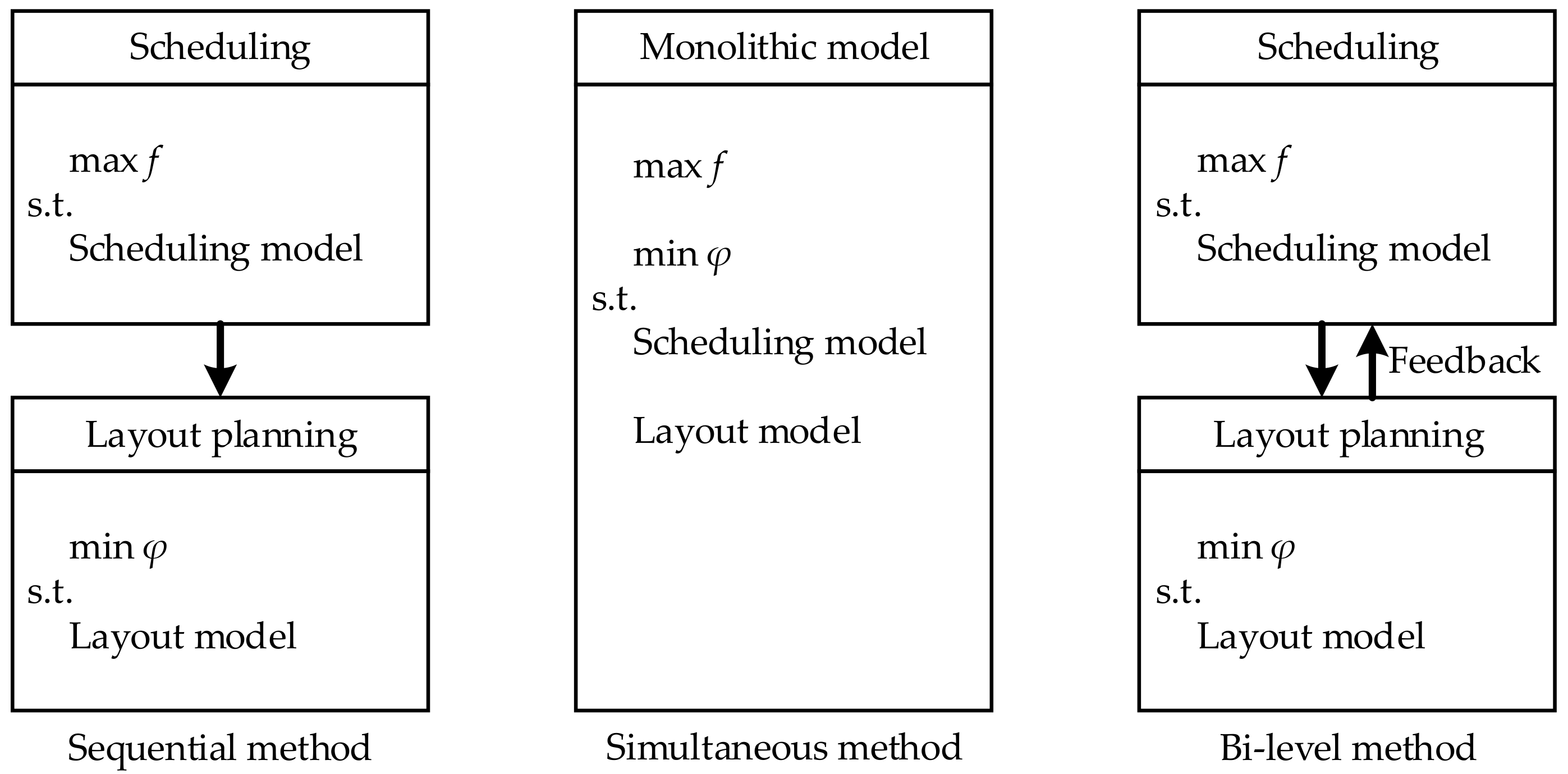
The possible solution strategies for the ISLP problem can be classified into three categories, as shown in Figure 2.
For the sequential method, the integrated problem is decomposed into two subproblems: one is the upper-level subproblem to determine scheduling schemes; the other is the lower-level subproblem to design corresponding layout schemes. The upper-level decisions are used as inputs for the lower-level subproblem. It is noted that the flow of information is only from the upper-level problem toward the lower-level problem. The sequential method is widely applied because of its simplicity, but it often results in a sub-optimal solution for the entire production process [27]. The sequential nature of the traditional approach prevents the scheduling model from considering detailed workshop layout information because the layout problem is not solved in the scheduling phase, which may lead to the scheduling scheme becoming inefficient and less practical. For example, a scheduling model often includes a parameter to denote the time required to process a job, but the actual completion time is highly dependent on the layout scheme, which influences the performance of the scheduling scheme.
In the simultaneous method, the layout model is simply appended to the scheduling model as constraints [10,15,16,17], which leads to the layout scheme lacking autonomy. Without its own objectives, the layout model is optimized to purse the objectives of the scheduling model. Nevertheless, in addition to considering the objectives of the scheduling problem, the layout problem also needs to achieve some objectives, such as the material handling cost, closeness rating score, space utilization ratio, and so on, to ensure the performance of the layout scheme. For the monolithic model only including scheduling objectives, it is difficult to consider the interaction of scheduling and layout planning. For example, if only the makespan of the scheduling problem is optimized, a scheduling scheme with minimum makespan may be executed difficultly in an unreasonable layout, resulting in frequent delays, interruptions, or failures in the operation process.
For the bi-level method, it can be regarded as a compromise between the sequential method and simultaneous method. Similar to the simultaneous method, it optimizes the scheduling and layout problems simultaneously as an integrated problem. Meanwhile, this method grants a degree of autonomy to the layout problems, so it has its own objectives. More importantly, the method enables collaboration between the scheduling problem and the layout problem by a feedback loop. Though the method outperforms the sequential and simultaneous methods in terms of the solution quality, the method encounters severe computational complexity [28]. Therefore, it is necessary to develop efficient algorithms to achieve this method.
In the proposed MEIFM problem, different from the previous literature [11,13,19], this paper considers flexible processing routes of jobs and unequal-area machines concurrently, which embodies a strong interaction between FJSSP and MRWLP. In addition, both FJSSP and MRWLP have independent objectives. Based on the characteristics of this problem and the description of the above three methods, it can be found that the bi-level method is a very efficient technique to tackle this MEIFM problem. In this method, the FJSSP and MRWLP represent two levels, with autonomy and independent objectives. More importantly, the bi-level method is flexible enough to consider the interaction of the FJSSP and MRWLP by the feedback loop. Therefore, the motivation of this study is using the hierarchical interaction characteristic of the FJSSP and MRWLP to search for a more effective model and solution for solving the complex integrated problem. In the next section, an MOBLP model for the proposed MEIFM problem is presented.
3. Bi-Level Programming Model for MEIFM
3.1. Problem Description
Based on the above description, the proposed MEIFM can be described as follows. In a given workshop, m rectangular machines are assigned to the multi-determined rows with the same height and n jobs are processed on these machines. Each job consists of a sequence of operations with known processing times, where each operation could be implemented on a set of machines. Different machines have different processing and idle energy consumption per unit time values. Besides this, using transporters to complete the transportation of jobs between machines and the number of transporters is unlimited. Each transporter has the same transportation energy consumption per unit time. The FJSSP aims to achieve the optimal scheduling scheme by assigning each operation to an appropriate machine (machine assignment problem) and determining a sequence of operations on all the machines (operation sequencing problem) for minimizing the makespan and total energy consumption, while the MRWLP aims to achieve the optimal layout scheme by determining the placement of all machines (machine location problem) for minimizing the material handling quantity. Note that the FJSSP and MRWLP are linked by material handling frequency and distance between machines, so they have a leader-follower coordinated structure. On the one hand, the FJSSP (leader)’s decision guides the optimization of the MRWLP (follower) by the material handling frequency between machines. On the other hand, the positions of machines determined by the layout scheme impact the transportation time and transportation energy consumption of jobs, which influences the performance of the scheduling scheme. Specifically, the integrated problem is shown in Figure 3. Moreover, to make the problem more concise, some assumptions should be satisfied, as shown below:
- (1)
- All jobs and machines are available at zero time, and machines can only be shut down if all jobs on them have been completed;
- (2)
- The job processing cannot be interrupted after starting processing, and each machine can only process one job at a time;
- (3)
- The loading and unloading time should be neglected in the process of jobs transportation;
- (4)
- The centers of machines located on the same row are in the same horizontal line;
- (5)
- The transportation time and energy consumption of jobs are only related to the distance between machines.
3.2. Model Formulation
Based on the above description, the paper formulates an MOBLP model to depict the proposed MEIFM problem. In the MOBLP, the “leader” in the upper-level is the FJSSP model, while the “follower” in the lower-level is the MRWLP model. The details of this coordinated optimization model are elaborated below.
3.2.1. Notations
This paper uses the following notations in the development of the mathematical model for the proposed MEIFM problem, as shown in Table 1.
3.2.2. Multi-Objective Bi-Level Programming Model
The structure of the proposed bi-level model is illustrated in Figure 4. In the structure, the upper-level model is linked to the lower-level model by flk and dlk. First, the lower-level model regards the flk of the upper-level model as constraints to optimize the layout scheme. Then, the dlk of the lower-level model feeds back to the upper-level model to affect the evaluation indexes of the upper-level model.
The upper-level model for FJSSP:
s.t.
Equations (1) and (2) are used to minimize the makespan and total energy consumption, respectively. It is noted that the total energy consumption includes the processing energy consumption and idle energy consumption of all machines, as well as the transportation energy consumption of all jobs. Equation (3) ensures that jobs are processed non-preemptively. Equation (4) guarantees that each machine can only process one job at a time. Equation (5) calculates the delay time of Oij on machine k. Figure 5 shows two cases of calculating dtijk, in which Figure 5a expresses that when cti’j’k is less than or equal to the sum of cti(j−1)l and ttlk, dtijk = 0 and Figure 5b shows that when cti’j’k is greater than the sum of cti(j−1)l and ttlk, dtijk = cti’j’k − ttlk − cti(j−1)l. Equation (6) calculates the transportation time of jobs between machines. Equation (7) calculates the start time of Oij on machine k. Equation (8) computes the material handling frequency between machines. Equation (9) calculates the idle time of each machine. Equations (10)–(12) are used to get the total processing energy consumption, total idle energy consumption, and total transportation energy consumption, respectively.
The lower-level model for MRWLP:
s.t.
Equation (13) is the objective function of the lower-level model, aiming to minimize the material handling quantity. Equations (14) and (15) calculate the horizontal coordinate and vertical coordinate of each machine in the workshop, respectively. Equation (16) calculates the distance between machine l and machine k. Equation (17) guarantees that the machines do not overlap in the horizontal direction. Equation (18) ensures that the vertical coordinates of the machines are identical in the same row. Equation (19) guarantees that each machine can only be located on one row. Equations (20)–(23) are boundary constraints, which indicates that each machine cannot exceed the workshop boundary. It is clear that the proposed MOBLP model is a mixed integer non-liner programming model.
4. Model Solution
4.1. Algorithm Construction
The MEIFM problem formulated in the previous section is a fairly challenging problem. First, the integrated problem is a bi-level program, which is an NP-hard problem [29]. Second, it essentially entails combinatorial optimization, which contains a lot of 0–1 decision variables and several complicated nonlinear constraints, resulting in this model becoming highly non-convex. Third, as the three objectives considered in this paper have different attributes and units, it is difficult to use traditional approaches to obtain a reasonable solution that balances production efficiency and energy consumption.
The traditional way of solving this kind of problem is to use Karush-Kuhn-Tucker (KKT) optimality conditions to replace the lower-level problem, which makes the bi-level programming model transform into a single-level model [30,31]. However, this approach can only solve a linear and convex lower-level problem, which makes the approach hard to apply in real-world problems, such as non-linearity, discreteness, non-convexity etc. To conquer these problems, many researchers directly simulate the decision-making process of bi-level programming by using the hierarchical optimization algorithm. Li et al. [22] designed a bi-level multi-objective particle swarm optimization algorithm to solve the dynamic construction site layout and security planning problem. Ma et al. [32] proposed a hierarchical hybrid particle swarm optimization and differential evolution algorithm to solve the pricing and lot-sizing decision problem. Miao et al. [33] developed a bi-level GA to solve the mixed integer nonlinear bi-level programming for the product family problem. As a representative intelligence algorithm, the genetic algorithm simulates the evolution process of survival of the fittest and approaches the excellent results gradually. It has great value for solving bi-level programming problems due to its better global searching performance and robust performance. Therefore, this paper proposes an IMHGA to divide the optimization process of the integrated problem into upper and lower levels. The upper-level NSGA-II is used to determine the optimal scheduling scheme by minimizing the Cmax and TEC, and the lower-level GA is employed to obtain the optimal layout scheme by minimizing the MHQ.
In the IMHGA, we design two improvement strategies to enhance the performance of the algorithm based on the characteristics of the MOBLP model. First, for the upper-level FJSSP, because its solution space is too large and the corresponding decision directly effects the optimization of the lower-level MRWLP, we need to find high-quality upper-level solutions as much as possible to guarantee the performance of the whole algorithm. However, it is difficult for the traditional NSGA-II algorithm to find an effective solution since most of the non-elitist solutions cannot fully participate in the genetic operation, which decreases the diversity of solutions and slows down the searching speed of the algorithm. To enhance the performance of the upper-level NSGA-II, we design the multi-parent improved precedence operation crossover (MIPOX) and multi-parent multipoint preservative crossover (MMPX) based on the multi-parent crossover method [34] for improving the quality of the Pareto solution set. The two crossovers not only satisfy the characteristics’ preservation and feasibility between parents and their children, but also enhance the global searching ability of the algorithm and improve the diversity of the solution by combining multiple parent information.
Second, for the lower-level MRWLP, its feedback directly impacts the evaluation of the upper-level FJSSP, so the convergence speed of the lower-level GA determines the convergence speed of the whole algorithm. Based on the concentration and diffusion strategy, once the scheduling scheme of the upper-level NSGA-II is determined, the lower-level GA will focus on finding the optimal layout scheme based on corresponding flk. Thus, to improve the convergence speed of the lower-level GA and find the optimal layout scheme, we adopt the tournament selection operator with the parent-offspring competition strategy as the selection operation. This selection operation can reserve elite individuals and conduct a centralized search of their neighborhood. Besides this, it can improve the convergence speed remarkably [35]. Specifically, the flowchart of IMHGA is given in Figure 6.
4.2. The Upper-Level Algorithm for FJSSP
4.2.1. Encoding and Initialization Population
Each scheduling scheme consists of two chromosomes: the operation sequence (OS) chromosome and the machine assignment (MA) chromosome. The OS chromosome represents the processing sequence of operations on machines and all operations belonging to the same job are denoted by the same index in the OS chromosome. The MA chromosome represents the machines assigned to the corresponding operations. Therefore, this chromosome representation method guarantees the feasibility of the scheduling schemes. For example, in Figure 7a, the number 2 written in the first gene of the OS chromosome is the first appearance of operation 2 in the sequence; therefore, it refers to operation 1 of job 2, i.e., O21. Similarly, the number 2 written in the fifth gene of the OS chromosome is the second appearance of operation 2, referring to operation 2 of job 2, i.e., O22. In Figure 7b, O11 written outside the first gene of the MA chromosome indicates that operation 1 of job 1 will be processed on machine 1. Similarly, O12 and O13 illustrate that operation 2 of job 1 will be processed on machine 4 and operation 3 of job 1 will be processed on machine 5.
Based on the above model introduction, the processing time of jobs has a significant impact on the upper-level algorithm. Therefore, in order to improve the quality of the initial population, this paper adopts an initial population generation strategy based on the processing time of jobs [36]. This approach considers the quality and diversity of the population. The basic idea is to randomly generate an OS chromosome, and then randomly select two machines from the corresponding available machine set for each operation. After that, the processing machine for each operation is determined by random numbers in the range of [0, 1]. If the random number is less than 0.8, the machine with a short processing time is selected; otherwise, another machine is chosen.
4.2.2. Fitness Evaluation
In the upper-level algorithm, the makespan and total energy consumption are directly used as the fitness evaluation criteria.
4.2.3. Selection Operator
The tournament selection is used as the selection operation in the upper-level algorithm, in which whether an individual is selected or not is determined by its non-dominated rank and crowding distance value. When we select two individuals randomly, the one which has a smaller non-dominated rank will be selected. When two individuals have the same non-dominated rank, we will select the individual with a higher crowding distance value.
4.2.4. Multi-Parent Crossover Operator
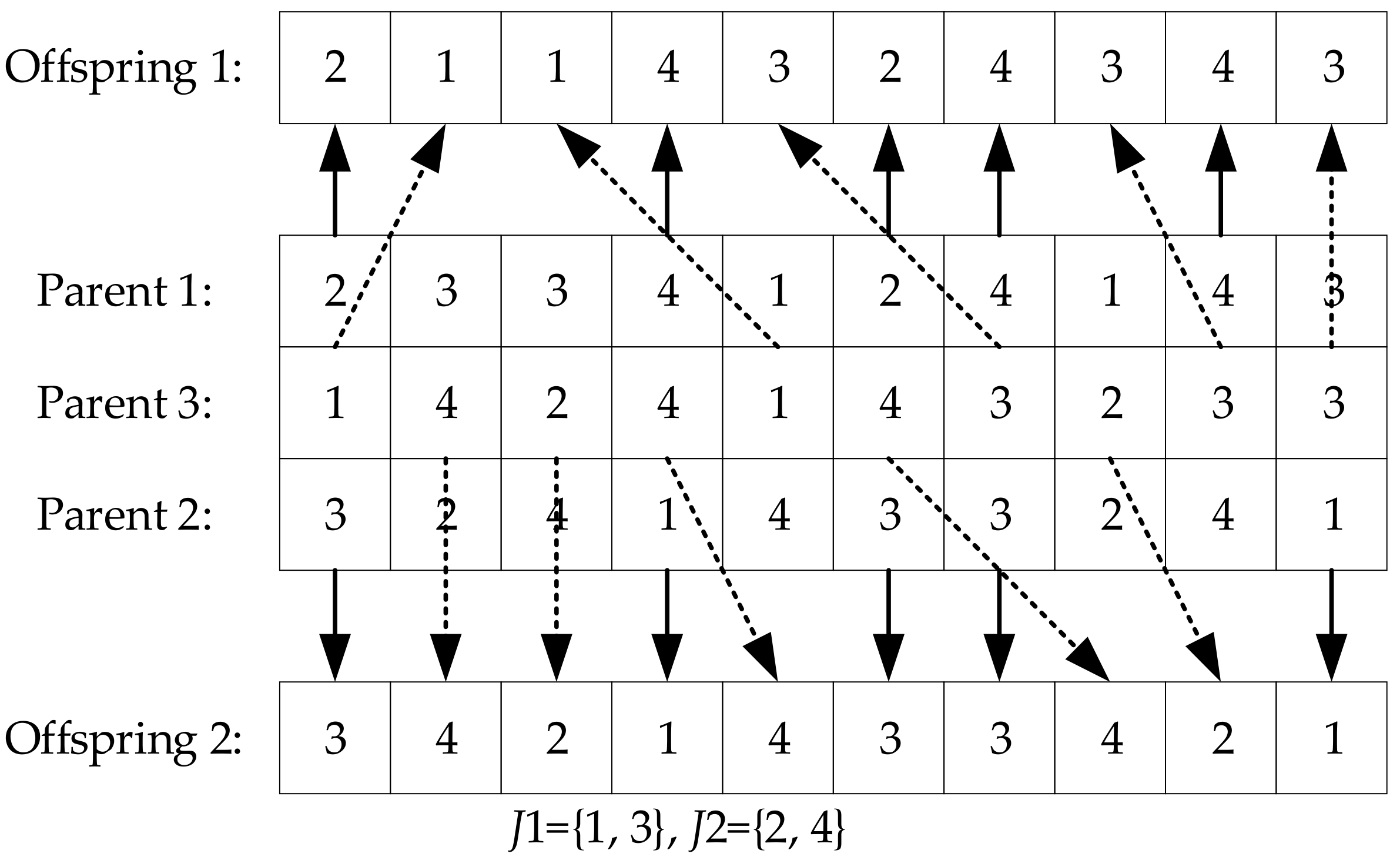
The performance of GA depends on the crossover operator to a large extent, which determines its global search capability. In traditional GA, the most common crossover operator uses two parents to produce offspring. Recently, multi-parent crossovers have attracted the attention of more and more researchers, and many studies have indicated the high performance of multi-parent crossover in some numerical optimization problems [37,38,39]. In the process of generating offspring, it is generally believed that multi-parent crossover is likely to synthesize more information of the parent individuals to obtain better search efficiency and higher quality solutions. Inspired by this crossover operation, to improve the global search efficiency of the algorithm and enhance the diversity of solutions, the multi-parent crossover is integrated with the improved precedence crossover (IPOX) [36,40] and multi-point preservative crossover (MPX) [41,42], and named MIPOX and MMPX, respectively.
The processes of the two designed crossover operators are described in Algorithms 1 and 2 separately and two examples are shown in Figure 8 and Figure 9, respectively.
| Algorithm 1 The procedure of MIPOX |
| Input: Three parent operation sequence chromosomes |
| Output: Two offspring operation sequence chromosomes |
| 1: Randomly divide the set of job numbers into two nonempty exclusive subsets J1 and J2; |
| 2: Copy those numbers in J2 from parent 1 to offspring 1 and from parent 3 to offspring 2, preserving their order; |
| 3: Copy those numbers in J1 from parent 2 to offspring 2 and from parent 3 to offspring 1, preserving their order. |
| Algorithm 2 The procedure of MMPX |
| Input: Three parent machine assignment chromosomes |
| Output: Two offspring machine assignment chromosomes |
| 1: Generate a random set Rand0_1, which consists of integer 0 and 1, and has the same length as machine assignment chromosomes; |
| 2: If Rand0_1 = 0, machine assignment number copies directly from Parent 1 to Offspring 1 and from Parent 2 to Offspring 2; |
| 3: If Rand0_1 = 1, machine assignment number copies randomly from Parent 2 and Parent 3 to Offspring 1 and from Parent 1 and Parent 3 to Offspring 2. |
4.2.5. Mutation Evaluation
In the upper level NSGA-II, two types of mutation are used: assignment mutation and swap mutation. The two mutation operators are applied to the selected chromosome and in the explained order (i.e., first assignment mutation and then swap mutation is applied). The assignment mutation is applied to the MA chromosome: a selected machine is replaced by another randomly chosen machine that can process the operation, while the swap mutation is applied to the OS chromosome: the randomly selected two genes are exchanged while maintaining the order of the operations of each job that guarantees that the mutated gene is a feasible solution.
4.3. The Lower-Level Algorithm for MRWLP
4.3.1. Encoding and Decoding
For the MRWLP, each chromosome in the lower-level GA consists of two parts, where one is the machine sequence chromosome and the other is the net distance chromosome between machines [43]. A complete layout scheme can be denoted as , , where the machine sequence chromosome indicates the processing priority of the machines by random number coding, and the net distance chromosome expresses the net distance between machines by real number coding.
4.3.2. Fitness Evaluation
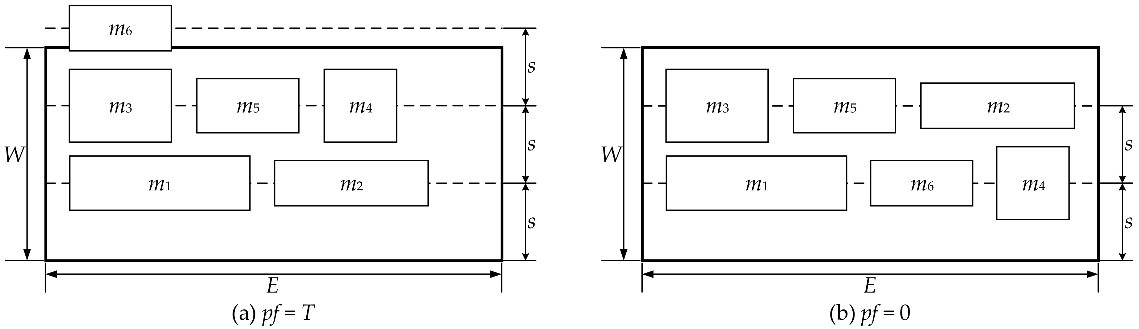
To reduce non-feasible solutions, this paper adds a penalty function with constraints to the fitness function. The fitness function of each chromosome in the lower-level population is shown below.
In Equations (24) and (25), pf is the penalty function and T is a large natural number. This paper adopts the automatic shift row strategy, which can ensure that all machines cannot exceed the workshop boundary in the horizontal direction. Therefore, it is only necessary to determine whether the last row of the machines exceeds the workshop boundary in the vertical direction. Figure 10 shows two examples of calculating fit. Figure 10a expresses that when the arrangements of machines exceed the workshop boundary in the vertical direction (rs > W), pf = T and fit = 1/(MHQ + T). Besides, Figure 10b shows that the arrangements of machines do not exceed the workshop boundary in the vertical direction, pf = 0 and fit = 1/MHQ.
4.3.3. Tournament Selection Operator with Parent-Offspring Competition Strategy
The paper adopts the tournament selection operator with the parent-offspring competition strategy to replace the traditional roulette wheel selection operator. In this selection operator, the parent population (Pl) and corresponding offspring population (Ol) constitute a temporary population (Tl). Then, the Tl is sorted according to the fitness value. Finally, the first Nl (the size of Pl) chromosomes are selected to form the next generation parent population (Pl+1), so as to ensure that the population size remains unchanged. The parent-offspring competition strategy not only preserves elite individuals and avoids loss of the best solution, but also improves the fitness of the overall population. The specific process is shown in Figure 11.
4.3.4. Crossover Operator
For crossover operation, this paper uses the partially mapped crossover operator (PMX) for machine sequence chromosomes and the arithmetic crossover operator for net distance chromosomes.
4.3.5. Mutation Operator
The mutation operator adopts the neighborhood search technique to find better offspring [44].
5. Computation Experiments
The IMHGA algorithm is coded in MATLAB R2018a and the experiments are run on an Intel (R) Core (TM) i7-7700HQ 2.8 Ghz process with 8 GB of memory under the Windows 10 operating system. To verify the effectiveness and efficiency of the proposed algorithm, we make comparisons with a general multi-objective hierarchical genetic algorithm (MHGA) from the perspectives of the convergence and distribution of the Pareto solution set.
5.1. Description of Test Data and Parameter Setting
Since the MEIFM problem is proposed for the first time and there is not a standard test set for it, in order to guarantee the validity and practicability of the proposed model and algorithm, the paper constructs a test data set by combining the data set available in the related and high-cited literature, instead of randomly generating a data set. Specifically, the jobs processing data [45] and corresponding machine energy consumption data [46] are shown in Table 2 and Table 3, separately, in which a solid line in a cell implies that machines is not available to perform that operation. The size of each machine [47] is shown in Table 4. Besides, these machines are located in a 17 m × 14 m workshop. The minimum distance between machines is 0.5 m and the minimum distance between machines and the workshop boundary is 1.5 m. The speed and energy consumption per unit time of transporter are 2 m/s and 5 kw, respectively.
In addition, the parameters of the proposed algorithm are determined after multiple trials. For the upper-level NSGA-II, the population size is 50, the maximal number of generations is 500, the crossover rate is 0.8, and the mutation rate is 0.1. For the lower-level GA, the population size is 40, the maximal number of generations is 100, the crossover rate is 0.8, and the mutation rate is 0.2.
5.2. Experimental Analyses
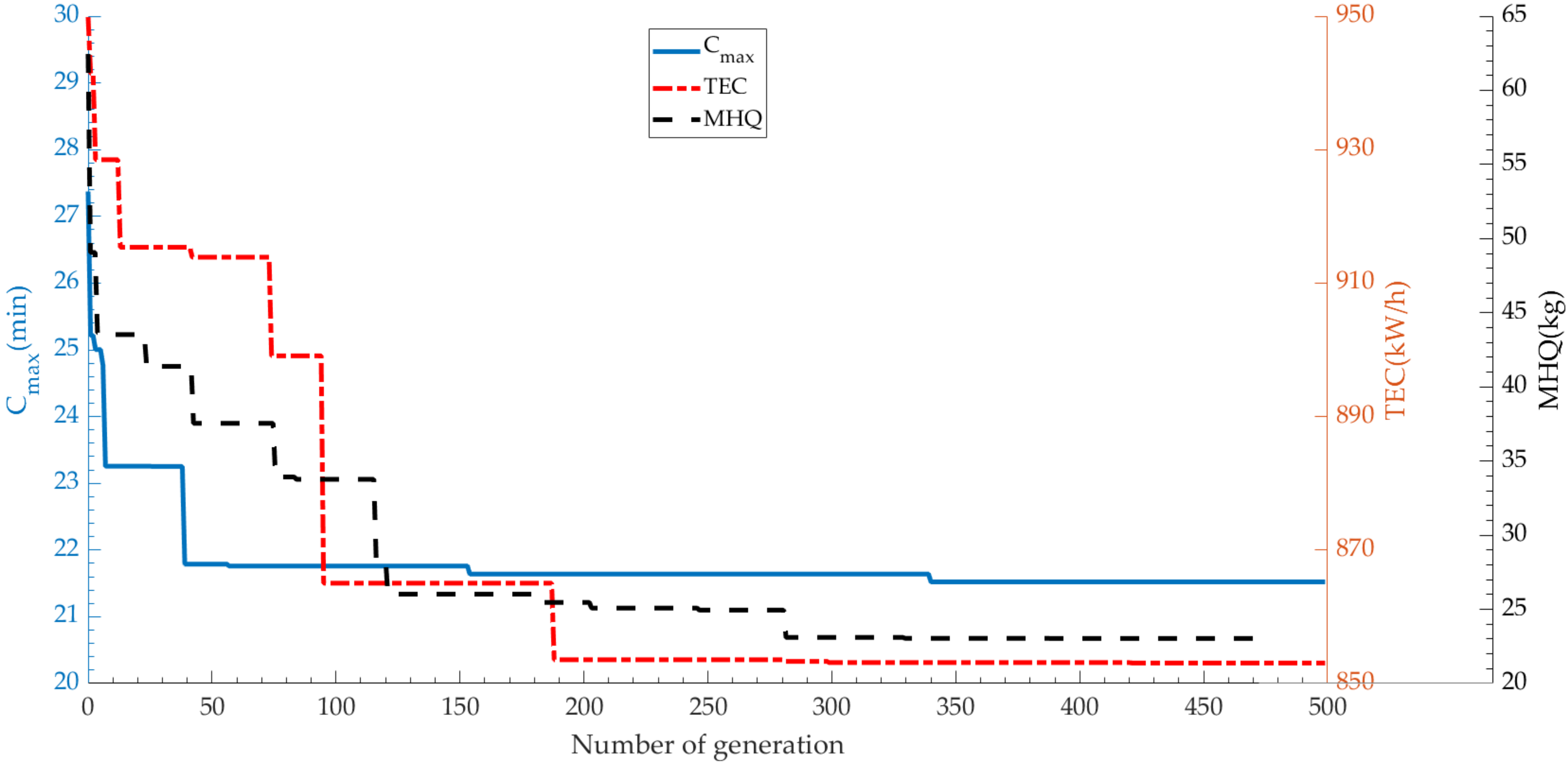
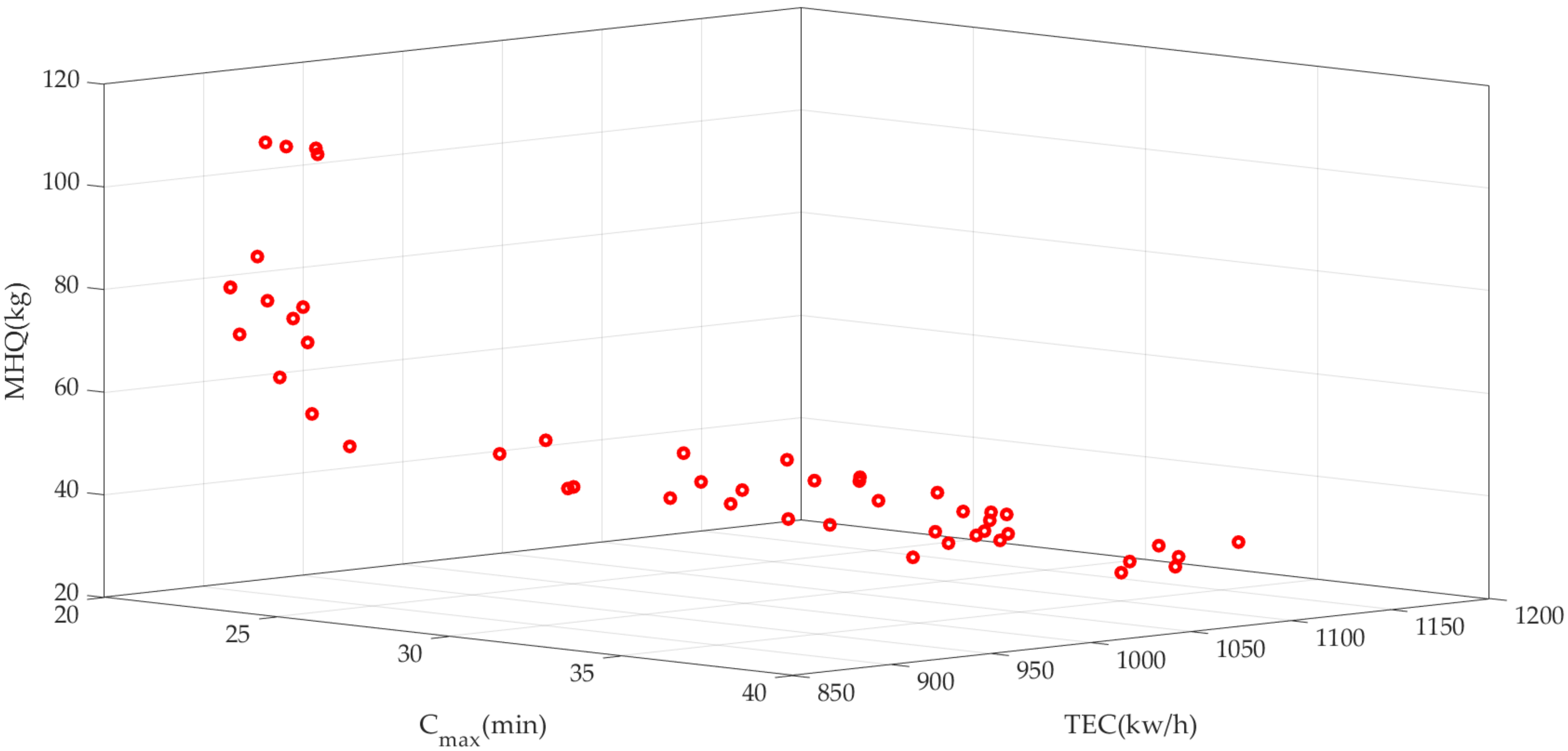
Figure 12 shows the convergence curves of three objectives, and these curves start to converge in the 280th generation. The Pareto solutions’ distributions of the final generation are shown in Figure 13, in which the same pareto solutions are plotted only once, and it can be seen that the Pareto solution set has a good distributivity. Thus, it can provide a wide range of alternative choices for the managers.
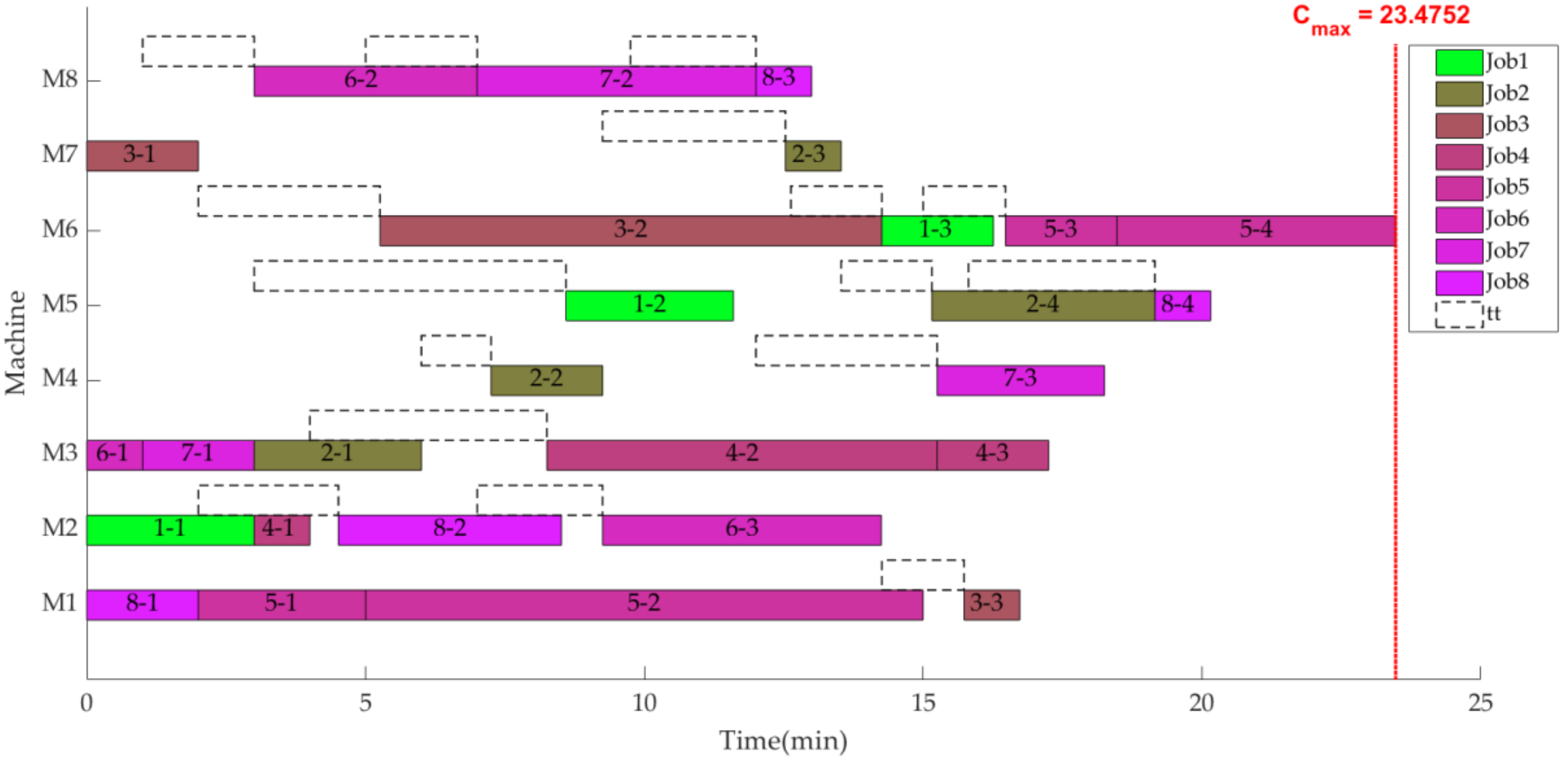
Moreover, Table 5 displays the three objectives and corresponding energy consumption components of part solutions in the Pareto solution set, where these solutions are ranked in non-increasing order of TEC. Figure 14 and Figure 15 give the scheduling gantt chart and workshop layout of solution 1, respectively, which shows that these solutions are logical and feasible. It can be seen that although the TEC of solution 1 is minimal in Pareto solutions, its energy consumption components (PE, IE, and TE) are not all minimal. This phenomenon implies that coordinated optimization of scheduling and layout planning is extremely important to reduce energy consumption for workshops.
In order to further analyze the relationship between TEC and corresponding energy consumption components (PE, IE, and TE), this paper uses the TEC of the Pareto solution set as the horizontal coordinate and the corresponding energy consumption components as the vertical coordinate to draw the distribution curve of each energy consumption component, as shown in Figure 16. It can be seen that the PE and TE curves are relatively stable, while the IE curve shows remarkable fluctuation. This is because the scheduling and layout planning determine the values of PE and TE, respectively, while the value of IE is affected by the scheduling and layout planning, which leads to the obvious fluctuation of the IE curve.
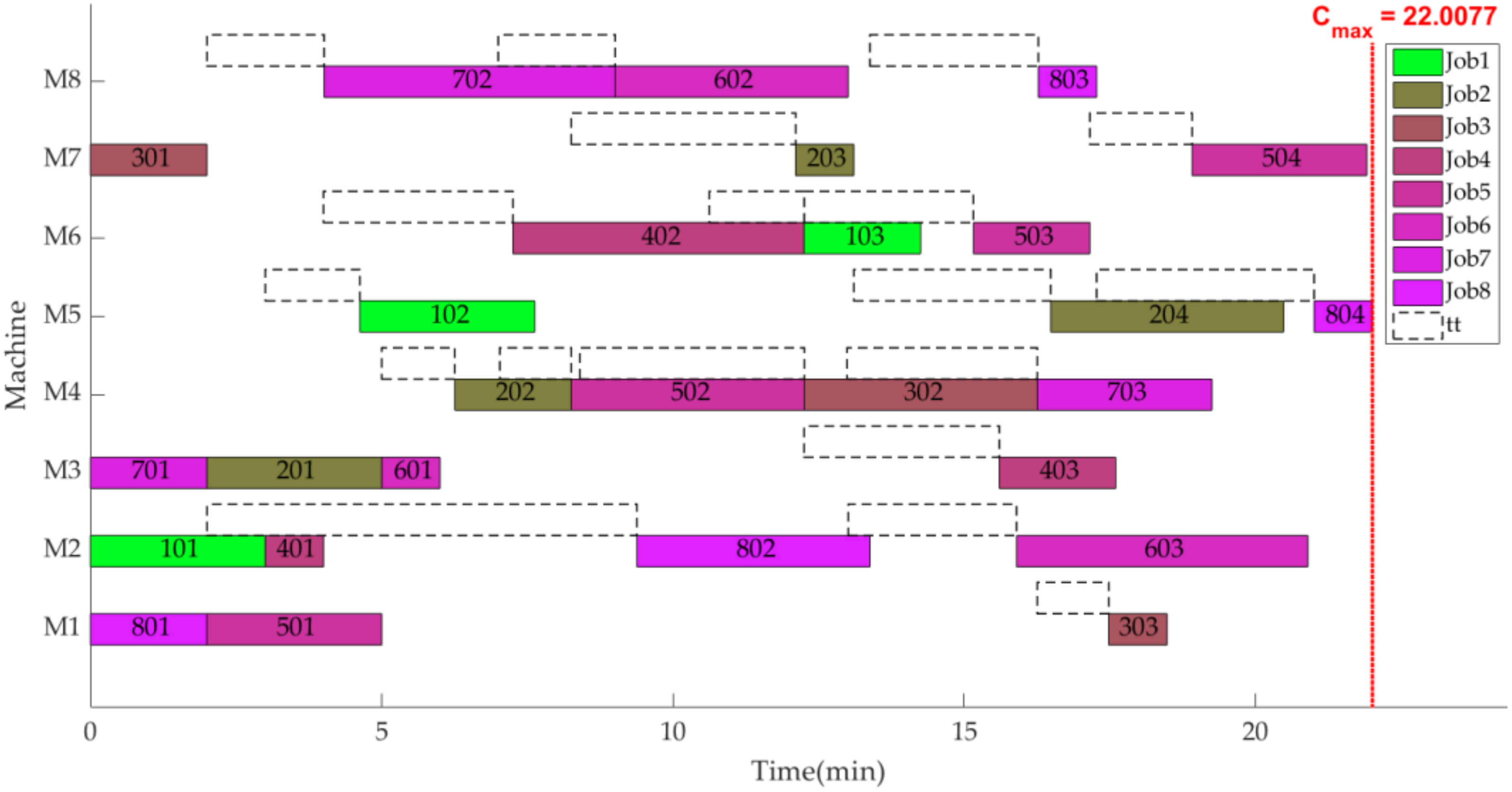
Moreover, in Figure 16, it is noted that the PE curve and TE curve correspond to a trough and a peak, respectively, when the TEC is about 900 kw/h. In order to explain this special phenomenon, the solutions related to this phenomenon are shown in Table 6. Figure 17 and Figure 18 show the scheduling gantt chart and workshop layout of the solution 13 in Table 6, respectively. Comparing Figure 14 with Figure 17, it can be found that although the Cmax and PE of solution 13 are less than solution 1, the TEC of solution 13 is still greater than that of solution 1. This is because each operation in solution 13 chooses the machine with a minimum processing time, which causes jobs to move frequently between machines, resulting in excessive TE and MHQ. Therefore, the PE and TE curves generate the peak-trough correspondence phenomenon. The phenomenon further illustrates that the coordinated optimization of scheduling and layout planning can not only quick respond to the changes of market demand, but also balance the production efficiency and energy consumption of enterprises.
5.3. Algorithm Comparison
In order to verify the effectiveness of the two improvement strategies, we compare the results of IMHGA with those of MHGA. In MHGA, the encoding scheme and mutation operator are the same as those in IMHGA, in which the operation sequence chromosome and machine assignment chromosome adopt IPOX and MPX as the crossover operator separately. Moreover, the parameters’ setting of the MHGA is the same as that of IMHGA.
In this paper, we adopt the convergence metric proposed by Zitzler et al. [48] and the spacing metric proposed by Schott et al. [49] to evaluate the convergence and distribution of Pareto solution sets, respectively. The two metrics are defined as follows.
Convergence metric: Compares the dominance relations between the pareto solutions obtained by the two algorithms to evaluate their convergence quality. It is assumed that X and Y are two pareto solutions obtained by the two algorithms. The dominance rate of X to Y can be expressed by the following formulation:
In Equation (26), |Y| is the number of solutions in the Y pareto solution set. The value C(X,Y) = 1, which means that all solutions in Y are dominated by or equal to solutions in X. On the contrary, if C(X,Y) = 0, this represents the situation when none of the solutions in Y are covered by the set X. It is noted that both C(X,Y) and C(Y,X) must be considered, since C(X,Y) is not necessarily equal to 1 − C(Y,X).
Spacing metric: Assumes that A is the Pareto solution set obtained by the algorithm. The formula for calculating the spacing metric is defined as follows.
In Equations (27) and (28), is the mean of all dzi, and |Z| is the number of solutions in the Z pareto solution set. If the metric is equal to zero, all solutions among the current Pareto front are equidistant.
Specifically, Figure 19 shows an example including two objectives to illustrate the above convergence and spacing metric. In the example, A and B are two pareto solutions obtained by different algorithms, in which A = [a1(1,7), a2(2, 4), a3(3, 3), a4(4, 2), a4(7, 1)] and B = [b1(2, 6), b2(3, 5), b3(4, 4), b4(5, 3), b5(6, 2)]. In Figure 19, it is obvious that the convergence of A is better than B and the distribution of B is better than A. From the perspective of the convergence metric, C(A,B) = 5/5 = 1 and C(B,A) = 0/5 = 0. Besides, from the perspective of the spacing metric, da1 = min{|1 − 2| + |7 − 4|, |1 − 3| + |7 − 3|, |1 − 4| + |7 − 2|, |1 − 7| + |7 − 1|} = min{4, 6, 8, 12} = 4; da2 = 2; da3 = 2; da4 = 2; da5 = 4; db1 = 2; db2 = 2; db3 = 2; db4 = 2; db5 = 2; = 2.8 and = 2. Accordingly, S(A) = = 1.0954 and S(B) = 0. It is clear that the results of the two metrics consist of the actual characterization of A and B, and illustrate that the larger the convergence value, the better the convergence, and the smaller spacing value, the better the distribution.
Table 7 shows the comparison results of the IMHGA and MHGA considering the metrics previously described. In Table 7, a solid line in a cell means a null value, which is a common practice. It can be seen that the Pareto solution set obtained by IMHGA is better than that by MHGA in terms of convergence and distribution, which illustrates the efficiency of MIPOX, MMPX, and the parent-offspring competition strategy.
6. Conclusions and Future Work
To improve the rapid response capability and save energy consumption for enterprises, we propose a novel MEIFM problem. FJSSP and MRWLP are traditionally addressed as two separate decisions, without considering the interaction between them. This paper focuses on the coordinated optimization between FJSSP and MRWLP, and integrates FJSSP and MRWLP decisions into a leader-follower decision framework. As a leader, the FJSSP aims at optimizing the performance of the scheduling scheme, while the MRWLP acts as a follower which responds to the leader’s decision on workshop layout. Furtherly, the paper proposes an MOBLP model to reveal the inherent bi-level structure in the MEIFM problem, which includes an upper-level model and a lower-level model. The upper-level model is FJSSP, which seeks the optimal scheduling scheme by minimizing the makespan and total energy consumption. The lower-level model is the MRWLP problem, which finds the optimal layout scheme by minimizing material handling quantity. As the integrated optimization problem is NP-hard, this paper proposes an IMHGA to solve it. The experimental results indicate that the proposed method can identify a set of Pareto optimal solutions with better convergence and distribution.
Based on the experimental results, the findings and implications are as follows:
- (1)
- Separate optimization of scheduling and layout planning can limit the performance of the manufacturing system because the interaction between them is ignored. Therefore, the coordination optimization of scheduling and layout planning is necessary and can greatly improve the compatibility of the manufacturing system;
- (2)
- The solutions of the MEIFM problem proposed by this paper not only improve the responsiveness of enterprises facing rapid changes of market demand, but also provide energy-saving methods from a systematic optimization perspective for manufacturing enterprises;
- (3)
- The methodology developed in this paper will provide efficient guidance and reference for solving complex bilevel optimization problems.
In the future, some other objectives, such as total tardiness, closeness rating score, and re-layout cost, should be considered when applying the proposed method. Besides, although the efficiency of this method is verified by the experimental results, its robustness and stability should be strengthened in future research.
Author Contributions
H.Z. contributed to the overall idea, algorithm, and writing of the manuscript; H.G. coded the algorithm in MATLAB and contributed to the detailed writing; R.P. contributed to the ideas and discussions on the integrated FJSSP and MRLP considering energy consumption, as well as the revision, preparation, and publishing of this paper; Y.W. analyzed the characteristics of the integrated optimization problem. All authors have read and approved the final manuscript.
Funding
This research is supported by the National Natural Science Foundation of China (Grant No. 71772002).
Conflicts of Interest
The authors declare no conflict of interest.
References
- Drira, A.; Pierreval, H.; Hajri-Gabouj, S. Facility layout problems: A survey. Annu. Rev. Control 2007, 31, 255–267. [Google Scholar] [CrossRef]
- Gupta, T.; Seifoddini, H. Production data based similarity coefficient for machine-component grouping decisions in the design of a cellular manufacturing system. Int. J. Prod. Res. 1990, 28, 1247–1269. [Google Scholar] [CrossRef]
- Ulutas, B.; Islier, A.A. Dynamic facility layout problem in footwear industry. J. Manuf. Syst. 2015, 36, 55–61. [Google Scholar] [CrossRef]
- Agency, I.E. Worldwide Trends in Energy Use and Efficiency; International Energy Agency (IEA): Paris, France, 2008. [Google Scholar]
- Jia, Z.H.; Zhang, Y.L.; Leung, Y.T.; Li, K. Bi-criteria ant colony optimization algorithm for minimizing makespan and energy consumption on parallel batch machines. Appl. Soft Comput. 2017, 55, 226–237. [Google Scholar] [CrossRef]
- Lei, D.; Zheng, Y.; Guo, X. A shuffled frog-leaping algorithm for flexible job shop scheduling with the consideration of energy consumption. Int. J. Prod. Res. 2017, 55, 3126–3140. [Google Scholar] [CrossRef]
- Mokhtari, H.; Hasani, A. An energy-efficient multi-objective optimization for flexible job-shop scheduling problem. Comput. Chem. Eng. 2017, 104, 339–352. [Google Scholar] [CrossRef]
- Yang, L.; Deuse, J.; Jiang, P. Multiple-attribute decision-making approach for an energy-efficient facility layout design. Int. J. Adv. Manuf. Technol. 2013, 66, 795–807. [Google Scholar] [CrossRef]
- Tayal, A.; Gunasekaran, A.; Singh, S.P.; Dubey, R.; Papadopoulos, T. Formulating and solving sustainable stochastic dynamic facility layout problem: A key to sustainable operations. Ann. Oper. Res. 2016, 253, 1–35. [Google Scholar] [CrossRef]
- Ranjbar, M.; Razavi, M.N. A hybrid metaheuristic for concurrent layout and scheduling problem in a job shop environment. Int. J. Adv. Manuf. Technol. 2011, 62, 1249–1260. [Google Scholar] [CrossRef]
- Ripon, K.S.N.; Glette, K.; Hovin, M.; Torresen, J. A multi-objective evolutionary algorithm for solving integrated scheduling and layout planning problems in manufacturing systems. In Proceedings of the 2012 IEEE Conference on Evolving and Adaptive Intelligent Systems (EAIS 2012), Madrid, Spain, 17–18 May 2012; pp. 157–163. [Google Scholar]
- Ripon, K.S.N.; Torresen, J. Integrated job shop scheduling and layout planning: A hybrid evolutionary method for optimizing multiple objectives. Evol. Syst. 2014, 5, 121–132. [Google Scholar] [CrossRef]
- Mallikarjuna, K.; Veeranna, V.; Reddy, K.H. A new meta-heuristics for optimum design of loop layout in flexible manufacturing system with integrated scheduling. Int. J. Adv. Manuf. Technol. 2015, 84, 1841–1860. [Google Scholar] [CrossRef]
- Liu, Q.; Zhao, H. Integrated optimization of workshop layout and scheduling to reduce carbon emissions based on a multi-objective fruit fly optimization algorithm. J. Mech. Eng. 2017, 53, 122–133. [Google Scholar] [CrossRef]
- Wu, X.; Chu, C.H.; Wang, Y.; Yue, D. Genetic algorithms for integrating cell formation with machine layout and scheduling. Comput. Ind. Eng. 2007, 53, 277–289. [Google Scholar] [CrossRef]
- Arkat, J.; Farahani, M.H.; Hosseini, L. Integrating cell formation with cellular layout and operations scheduling. Int. J. Adv. Manuf. Technol. 2011, 61, 637–647. [Google Scholar] [CrossRef]
- Fahmy, S.A. Mixed integer linear programming model for integrating cell formation, group layout and group scheduling. In Proceedings of the IEEE International Conference on Industrial Technology, Seville, Spain, 17–19 March 2015; pp. 2403–2408. [Google Scholar]
- Arkat, J.; Farahani, M.H.; Ahmadizar, F. Multi-objective genetic algorithm for cell formation problem considering cellular layout and operations scheduling. Int. J. Comput. Integr. Manuf. 2012, 25, 625–635. [Google Scholar] [CrossRef]
- Suemitsu, I.; Izui, K.; Yamada, T.; Nishiwaki, S.; Noda, A.; Nagatani, T. Simultaneous optimization of layout and task schedule for robotic cellular manufacturing systems. Comput. Ind. Eng. 2016, 102, 396–407. [Google Scholar] [CrossRef]
- Lu, K.; Li, T.; Wang, K.; Zhu, H.; Makoto, T.; Yu, B. An improved shuffled frog-leaping algorithm for flexible job shop scheduling problem. Algorithms 2015, 8, 19–31. [Google Scholar] [CrossRef]
- Hungerländer, P.; Anjos, M.F. A semidetermined optimization-based approach for global optimization of multi-row facility layout. Eur. J. Oper. Res. 2015, 245, 46–61. [Google Scholar] [CrossRef]
- Li, Z.; Shen, W.; Xu, J.; Lev, B. Bilevel and multi-objective dynamic construction site layout and security planning. Autom. Constr. 2015, 57, 1–16. [Google Scholar] [CrossRef]
- Sinha, A.; Deb, K. Towards understanding evolutionary bilevel multi-objective optimization algorithm. In IFAC Workshop on Control Applications of Optimization (IFAC-2009); IFAC: Prague, Czech Republic, 2009; Volume 42, pp. 338–343. [Google Scholar]
- Sinha, A.; Malo, P.; Deb, K.; Korhonen, P.; Wallenius, J. Solving bilevel multicriterion optimization problems with lower level decision uncertainty. IEEE Trans. Evol. Comput. 2016, 20, 199–217. [Google Scholar] [CrossRef]
- Sinha, A.; Malo, P.; Deb, K. Towards understanding bilevel multi-objective optimization with deterministic lower level decisions. In Proceedings of the 8th International Conference on Evolutionary Multi-Criterion Optimization (EMO), Guimaraes, Portugal, 29 March–1 April 2015; pp. 426–443. [Google Scholar]
- Lu, Z.; Deb, K.; Goodman, E.; Wassick, J. Solving a supply-chain management problem using a bilevel approach. In Proceedings of the Genetic and Evolutionary Computation Conference, Berlin, Germany, 15–19 July 2017; pp. 1185–1192. [Google Scholar]
- Chu, Y.; You, F.; Wassick, J.M.; Agarwal, A. Integrated planning and scheduling under production uncertainties: Bi-level model formulation and hybrid solution method. Comput. Chem. Eng. 2015, 72, 255–272. [Google Scholar] [CrossRef]
- Chu, Y.; You, F. Integrated scheduling and dynamic optimization by stackelberg game: Bilevel model formulation and efficient solution algorithm. Ind. Eng. Chem. Res. 2016, 53, 5564–5581. [Google Scholar] [CrossRef]
- Colson, B.; Marcotte, P.; Savard, G. An overview of bilevel optimization. Ann. Oper. Res. 2007, 153, 235–256. [Google Scholar] [CrossRef]
- Miao, C.; Du, G.; Jiao, R.J.; Zhang, T. Coordinated optimisation of platform-driven product line planning by bilevel programming. Int. J. Prod. Res. 2017, 55, 3808–3831. [Google Scholar] [CrossRef]
- Aghajani, S.; Kalantar, M. Operational scheduling of electric vehicles parking lot integrated with renewable generation based on bilevel programming approach. Energy 2017, 139, 422–432. [Google Scholar] [CrossRef]
- Ma, W.; Wang, M.; Zhu, X. Hybrid particle swarm optimization and differential evolution algorithm for bi-level programming problem and its application to pricing and lot-sizing decisions. J. Intell. Manuf. 2015, 26, 471–483. [Google Scholar] [CrossRef]
- Miao, C.; Du, G.; Xia, Y.; Wang, D. Genetic algorithm for mixed integer nonlinear bilevel programming and applications in product family design. Math. Probl. Eng. 2016, 16, 1–15. [Google Scholar] [CrossRef]
- Khuat, T.T.; Le, M.H. A genetic algorithm with multi-parent crossover using quaternion representation for numerical function optimization. Appl. Intell. 2016, 46, 810–826. [Google Scholar] [CrossRef]
- Wang, C.; Zhao, A.; Dong, H.; Li, Z. An improved immune genetic algorithm for distribution network reconfiguration. In Proceedings of the 2nd International Conference on Information Management, Innovation Management and Industrial Engineering, Xi’an, China, 26–27 December 2009; pp. 218–223. [Google Scholar]
- Wang, X.; Gao, L.; Zhang, C.; Shao, X. A multi-objective genetic algorithm based on immune and entropy principle for flexible job-shop scheduling problem. Int. J. Adv. Manuf. Technol. 2010, 51, 757–767. [Google Scholar] [CrossRef]
- Bégin-Drolet, A.; Collin, S.; Gosselin, J.; Ruel, J. A new robust controller for non-linear periodic single-input/single-output systems using genetic algorithms. J. Process Control 2018, 61, 23–35. [Google Scholar] [CrossRef]
- Bouchekara, H.R.E.H.; Chaib, A.E.; Abido, M.A. Optimal power flow using GA with a new multi-parent crossover considering: Prohibited zones, valve-point effect, multi-fuels and emission. Electr. Eng. 2016, 100, 151–165. [Google Scholar] [CrossRef]
- Elsayed, S.M.; Sarker, R.A.; Essam, D.L. GA with a New Multi-Parent Crossover for Constrained Optimization. In Proceedings of the IEEE Congress on Evolutionary Computation (CEC), New Orleans, LA, USA, 5–8 June 2011; pp. 857–864. [Google Scholar]
- Wang, X.; Gao, L.; Zhang, C.; Li, X. A multi-objective genetic algorithm for fuzzy flexible job-shop scheduling problem. Int. J. Comput. Appl. Technol. 2012, 45, 115–125. [Google Scholar] [CrossRef]
- Türkyılmaz, A.; Bulkan, S. A hybrid algorithm for total tardiness minimisation in flexible job shop: Genetic algorithm with parallel VNS execution. Int. J. Prod. Res. 2015, 53, 1832–1848. [Google Scholar] [CrossRef]
- Zheng, X.L.; Wang, L.; Wang, S.Y. A novel fruit fly optimization algorithm for the semiconductor final testing scheduling problem. Knowl.-Based. Syst. 2014, 57, 95–103. [Google Scholar] [CrossRef]
- Miao, Z.; Xu, K.L. Research of multi-rows facility layout based on hybrid algorithm. In Proceedings of the 2nd International Conference on Information Management, Innovation Management and Industrial Engineering, Xi’an, China, 26–27 December 2009; pp. 553–556. [Google Scholar]
- Gen, M.; Ida, K.; Cheng, C. Multirow machine layout problem in fuzzy environment using genetic algorithms. Comput. Ind. Eng. 1995, 29, 519–523. [Google Scholar] [CrossRef]
- Zhang, C. Improved NSGA-II for the multi-objective flexible job-shop scheduling problem. J. Mech. Eng. 2010, 46, 156–164. [Google Scholar] [CrossRef]
- Lei, W.; Cai, J.; Xin, S. Multi-objective flexible job shop energy-saving scheduling problem based on improved genetic algorithm. J. Nanjing Univ. Sci. Technol. 2017, 41, 494–502. [Google Scholar]
- Zhang, Y.; Lu, C.; Zhang, H.; Fang, Z.F. Workshop layout optimization based on differential cellular multi-objective genetic algorithm. Comput. Integr. Manuf. 2013, 19, 727–734. [Google Scholar]
- Zitzler, E.; Deb, K.; Thiele, L. Comparison of multiobjective evolutionary algorithms: Empirical results. Evol. Comput. 2000, 8, 173–195. [Google Scholar] [CrossRef]
- Schott, J.R. Fault Tolerant Design Using Single and Multi-Criteria Genetic Algorithms. Ph.D. Dissertation, Massachusetts Institute of Technology, Cambridge, MA, USA, 1995. [Google Scholar]
Figure 1.
Relations between FJSSP and MRWLP.

Figure 2.
Structures of three methods for solving the ISLP problem.

Figure 3.
Leader-follower coordinated structure of the MEIFM problem.

Figure 4.
Structure of the proposed bi-level model.

Figure 5.
Two cases of calculating dtijk.

Figure 6.
The flowchart of IMHGA.

Figure 7.
A chromosome example for the scheduling scheme.

Figure 8.
An example for MIPOX.

Figure 9.
An example for MMPX.

Figure 10.
Two examples of calculating fit.

Figure 11.
Tournament selection operator with the parent-offspring competition strategy.

Figure 12.
The convergence curve of three objective functions.

Figure 13.
The Pareto solutions’ distribution for three objective functions.

Figure 14.
The Gantt chart of solution 1.

Figure 15.
The layout scheme of solution 1.

Figure 16.
The distribution curves for three energy consumption components.

Figure 17.
The Gantt chart of solution 13.

Figure 18.
The layout scheme of solution 13.

Figure 19.
An example of calculating the convergence and spacing metric.


Table 1.
The notations used in this paper.
| Symbol | Meaning | |
|---|---|---|
| Optimization objectives | Cmax | Makespan |
| TEC | Total energy consumption | |
| MHQ | Material handling quantity | |
| Index | i | Index of job, i = 1, 2, , n |
| j | Index of operation for job i, j = 1, 2, , oi | |
| k, l | Index of machine, k, l = 1, 2, , m | |
| r | Index of machine row number, r = 1, 2, , g | |
| Intermediate variables | Oij | j-th operation of the job i |
| ctijk | Completion time of Oij on machine k | |
| cti’j’k | Completion time of immediate operation of Oij on machine k | |
| stijk | Start time of Oij on machine k | |
| itk | Idle time of machine k | |
| ttlk | Transportation time from machine l to machine k | |
| dtijk | Delay time of Oij on machine k due to machine resource constraints | |
| dlk | Distance between machine l to machine k | |
| flk | Material handling frequency from machine l to machine k | |
| PE | Processing energy consumption of all machines | |
| IE | Idle energy consumption of all machines | |
| TE | Transportation energy consumption of all jobs in workshop | |
| xl | Horizontal coordinate of machine l in workshop | |
| yl | Vertical coordinate of machine l in workshop | |
| Input variables | ptijk | Processing time of Oij on machine k |
| v | Transportation speed of transporter in workshop | |
| pek | Processing energy consumption per unit time of machine k | |
| iek | Idle energy consumption per unit time of machine k | |
| te | Transportation energy consumption per unit time of transporter | |
| elk | Minimal distance between machine l and machine k that must be maintained in horizontal direction | |
| Δlk | Net distance between machine l and machine k in horizontal direction | |
| el | Length of machine l in horizontal direction | |
| wl | Width of machine l in vertical direction | |
| s | Center distance of two adjacent rows | |
| E | Length of workshop in horizontal direction | |
| W | Width of workshop in vertical direction | |
| Decision variables | xijk | Binary variable, if Oij is processed on machine k, then xijk = 1; otherwise, xijk = 0 |
| xilk | Binary variable, if job i is transported from machine l to machine k, then xilk = 1; otherwise, xilk = 0 | |
| zlr | Binary variable, if machine l is located on r-th row in the workshop, then zlr = 1; otherwise zlr = 0 | |
Table 2.
Processing time of jobs.
| Job | Operation | Processing Time (min) | |||||||
|---|---|---|---|---|---|---|---|---|---|
| M1 | M2 | M3 | M4 | M5 | M6 | M7 | M8 | ||
| Job 1 | O1,1 | 5 | 3 | 5 | 3 | 3 | — | 10 | 9 |
| O1,2 | 10 | — | 5 | 8 | 3 | 9 | 9 | 6 | |
| O1,3 | — | 10 | — | 5 | 6 | 2 | 4 | 5 | |
| Job 2 | O2,1 | 5 | 7 | 3 | 9 | 8 | — | 9 | — |
| O2,2 | — | 8 | 5 | 2 | 6 | 7 | 10 | 9 | |
| O2,3 | — | 10 | — | 5 | 6 | 4 | 1 | 7 | |
| O2,4 | 10 | 8 | 9 | 6 | 4 | 7 | — | — | |
| Job 3 | O3,1 | 10 | — | — | 7 | 6 | 5 | 2 | 4 |
| O3,2 | — | 10 | 6 | 4 | 8 | 9 | 10 | — | |
| O3,3 | 1 | 4 | 5 | 6 | — | 10 | — | 7 | |
| Job 4 | O4,1 | 3 | 1 | 6 | 5 | 9 | 7 | 8 | 4 |
| O4,2 | 12 | 11 | 7 | 8 | 10 | 5 | 6 | 9 | |
| O4,3 | 4 | 6 | 2 | 10 | 3 | 9 | 5 | 7 | |
| Job 5 | O5,1 | 3 | 6 | 7 | 8 | 9 | — | 10 | — |
| O5,2 | 10 | — | 7 | 4 | 9 | 8 | 6 | — | |
| O5,3 | — | 9 | 8 | 7 | 4 | 2 | 7 | — | |
| O5,4 | 11 | 9 | — | 6 | 7 | 5 | 3 | 6 | |
| Job 6 | O6,1 | 6 | 7 | 1 | 4 | 6 | 9 | — | 10 |
| O6,2 | 11 | — | 9 | 9 | 9 | 7 | 6 | 4 | |
| O6,3 | 10 | 5 | 9 | 10 | 11 | — | 10 | — | |
| Job 7 | O7,1 | 5 | 4 | 2 | 6 | 7 | — | 10 | — |
| O7,2 | — | 9 | — | 9 | 11 | 9 | 10 | 5 | |
| O7,3 | — | 8 | 9 | 3 | 8 | 6 | — | 10 | |
| Job 8 | O8,1 | 2 | 8 | 5 | 9 | — | 4 | — | 10 |
| O8,2 | 7 | 4 | 7 | 8 | 9 | — | 10 | — | |
| O8,3 | 9 | 9 | — | 8 | 5 | 6 | 7 | 1 | |
| O8,4 | 9 | — | 3 | 7 | 1 | 5 | 8 | — | |
Table 3.
The energy consumption per unit time of machines.
| Machine Number | M1 | M2 | M3 | M4 | M5 | M6 | M7 | M8 | |
|---|---|---|---|---|---|---|---|---|---|
| Energy Consumption | |||||||||
| pek (kw) | 4.0 | 7.0 | 9.0 | 14.0 | 6.0 | 5.0 | 8.0 | 4.0 | |
| iek (kw) | 1.0 | 1.2 | 0.9 | 0.8 | 0.6 | 0.9 | 0.8 | 0.8 | |
Table 4.
The size of each machine.
| Machine Number | M1 | M2 | M3 | M4 | M5 | M6 | M7 | M8 | |
|---|---|---|---|---|---|---|---|---|---|
| Size | |||||||||
| ek (m) | 1.9 | 3.0 | 2.0 | 2.0 | 2.5 | 3.0 | 3.0 | 5.0 | |
| wk (m) | 1.8 | 2.0 | 1.0 | 1.8 | 1.5 | 3.0 | 2.8 | 3.0 | |
Table 5.
The Pareto set.
| Solution Number | Cmax (min) | TEC (kw/h) | MHQ (kg) | PE (kw/h) | IE (kw/h) | TE (kw/h) |
|---|---|---|---|---|---|---|
| 1 | 23.4752 | 853.0703 | 82.8975 | 562 | 83.8266 | 207.2437 |
| 2 | 23.4752 | 853.2411 | 82.9660 | 562 | 83.8260 | 207.4151 |
| 3 | 23.5124 | 857.1738 | 73.6347 | 592 | 81.0870 | 184.0868 |
| 4 | 23.4751 | 866.7355 | 88.3640 | 562 | 83.8254 | 220.9101 |
| 5 | 23.4794 | 871.7218 | 79.5463 | 592 | 80.8560 | 198.8658 |
| 46 | 33.3751 | 1133.8233 | 24.9989 | 952 | 119.3260 | 62.4973 |
| 47 | 33.3750 | 1148.3944 | 27.4677 | 954 | 125.7250 | 68.6693 |
| 48 | 33.3838 | 1156.5963 | 23.0329 | 978 | 120.9869 | 57.5823 |
| 49 | 33.3769 | 1158.3316 | 24.8773 | 978 | 118.1384 | 62.1932 |
| 50 | 33.3750 | 1188.4205 | 26.4382 | 1004 | 118.3250 | 66.0955 |
Table 6.
The solutions in the trough and the peak.
| Solution Number | Cmax (min) | TEC (kw/h) | MHQ (kg) | PE (kw/h) | IE (kw/h) | TE (kw/h) |
|---|---|---|---|---|---|---|
| 13 | 22.0077 | 904.4978 | 107.4975 | 550 | 85.7541 | 268.7437 |
| 14 | 21.5220 | 906.5748 | 106.9683 | 550 | 89.1541 | 267.4207 |
| 15 | 22.7642 | 909.2554 | 105.9224 | 550 | 94.4495 | 264.8059 |
| 16 | 22.6255 | 910.7705 | 106.9167 | 550 | 93.4788 | 267.2918 |
Table 7.
Result of the evaluation metrics of the IMHAG and MHGA.
| Algorithm | Convergence Metric | Spacing Metric | |
|---|---|---|---|
| C(IMHGA, MHGA) | C(MHGA, IMHGA) | ||
| IMHGA | 0.9338 | — | 3.2292 |
| MHGA | — | 0.2000 | 5.9856 |
© 2018 by the authors. Licensee MDPI, Basel, Switzerland. This article is an open access article distributed under the terms and conditions of the Creative Commons Attribution (CC BY) license (http://creativecommons.org/licenses/by/4.0/).
Share and Cite
MDPI and ACS Style
Zhang, H.; Ge, H.; Pan, R.; Wu, Y. Multi-Objective Bi-Level Programming for the Energy-Aware Integration of Flexible Job Shop Scheduling and Multi-Row Layout. Algorithms 2018, 11, 210. https://0-doi-org.brum.beds.ac.uk/10.3390/a11120210
AMA Style
Zhang H, Ge H, Pan R, Wu Y. Multi-Objective Bi-Level Programming for the Energy-Aware Integration of Flexible Job Shop Scheduling and Multi-Row Layout. Algorithms. 2018; 11(12):210. https://0-doi-org.brum.beds.ac.uk/10.3390/a11120210
Chicago/Turabian StyleZhang, Hongliang, Haijiang Ge, Ruilin Pan, and Yujuan Wu. 2018. "Multi-Objective Bi-Level Programming for the Energy-Aware Integration of Flexible Job Shop Scheduling and Multi-Row Layout" Algorithms 11, no. 12: 210. https://0-doi-org.brum.beds.ac.uk/10.3390/a11120210
Note that from the first issue of 2016, this journal uses article numbers instead of page numbers. See further details here.